The Period Function of the Generalized Sine-Gordon Equation and the Sinh-Poisson Equation

Abstract

In this paper, we consider the generalized sine-Gordon equation ${\psi }_{tx}=(1+a{\partial }_x^2)\sin \psi$ and the sinh-Poisson equation $u_{xx}+u_{yy}+\sigma \sinh u=0$, where a is a real parameter, and $\sigma$ is a positive parameter. Under different conditions, e.g., $a=0$, $a\ne 0$, and $\sigma >0$, the periods of the periodic wave solutions for the above two equations are discussed. By the transformation of variables, the generalized sine-Gordon equation and sinh-Poisson equations are reduced to planar dynamical systems whose first integral includes trigonometric terms and exponential terms, respectively. We successfully handle the trigonometric terms and exponential terms in the study of the monotonicity of the period function of periodic solutions.

1. Introduction

The sine-Gordon (sG) equation is a non-linear partial differential equation mainly applied in various fields of theoretical physics, including condensed matter physics, particle physics, and non-linear optics [1,2,3,4]. The sinh-Poisson (sP) equation has been used to study steady-state flows in an ideal incompressible liquid [5] and the dynamic behaviors of Kolmogorov flow. Cellular structures with square or hexagonal cells and quasi-crystal patterns of the sP equation are investigated in [6]. In this paper, we consider the generalized sG equation

$${\psi }_{tx}=(1+a{\partial }_x^2)\sin \psi ,$$

(1)

and the sP equation

$$u_{xx}+u_{yy}+\sigma \sinh u=0,$$

(2)

where a is a real parameter, $\psi (x,t)$, is a scalar valued function, $u(x,y)$ represents the electrostatic potential, and $\sigma$ is a positive parameter related to the plasma density and temperature.

In 1995, Fokas [7] first derived Equation (1) using the bi-Hamiltonian method. When $a=0,$ Equation (1) becomes the standard sG equation. Ling and Sun [8] found multi-elliptic localized solutions, such as multi-elliptic kink solutions, multi-elliptic breather solutions, and multi-elliptic kink–breather solutions, using the Darboux–Bäcklund transformation method for $a=0.$ When $a\ne 0$, many scholars have been devoted to study the dynamic behaviors of solitary waves in Equation (1). In the case where $a<0$, Equation (1) can be transformed into the sG equation using an appropriate Liouville-type transformation, and the behaviors of cusped and anti-cusped traveling-wave solutions to Equation (1) are discussed using conservation laws [9]. For $a=-1$, Matsuno [10] constructed multi-soliton solutions in the form of parametric representation, and obtained many different solutions such as kinks, loop solitons, and breathers. For $a=1$, Matsuno [11] found that Equation (1) has kink and breather solutions but cannot have multi-valued solutions like loop solitons, as obtained in Ref. [10]. Gatlik et al. [12] studied the kink–inhomogeneity interaction for an sG equation. Carretero-González et al. [13] analyzed the interaction dynamics between kink and anti-kink stripes in a 2D sG equation. The integrable discretized system of Equation (1) has also been investigated. For instance, Feng et al. [14] constructed N-soliton solutions for the semi-discrete analogues of Equation (1) in the determinant form. In the continuous limit, they showed that the semi-discrete, generalized sG equation converged to the continuous generalized sG Equation (1). Sheng et al. [15] further found that in continuous, semi-discrete, and fully discrete cases, the generalized sG equation can be reduced into a short pulse equation. Xiang et al. [16] obtained some solutions and continuum limits to non-local, discrete sG equations using the bilinearization reduction method. Recently, Lührmann and Schlag [17] discussed the asymptotic stability of the kink solution for the sG equation under odd perturbations.

The sP Equation (2) originates from the mean field limit of ideal parallel line vortices with numerous interactions, and this model depicts a stream function configuration of a stationary 2D Euler flow [18]. Moreover, the sP Equation (2) is closely related to the long-time state of the 2D Navier–Stokes flow and some integrable soliton models, and the exact solutions of this equation play an important role in theoretic study and practice applications [19]. In past decades, the existence and multiplicity of solutions for Equation (2) have been investigated extensively, and the research topics involved equilibria and stability [20], boundary value problems [21,22], numerical calculations [23], and sign-changing solutions [24,25]. When $\sigma$ was a sufficiently small positive constant, Bartolucci and Pistoia [26] obtained that Equation (2) has two pairs of nodal solutions under Dirichlet boundary conditions.

Currently, there is relatively little research on the behaviors of the periodic solutions of the sG equation and the sP equation. An important feature of the sG equation and sP equation is that both equations have soliton solutions and periodic solutions. A periodic solution is a special type of solution for non-linear wave equations, which is essentially different from the propagation of solitary wave solutions. In 2015, Li and Qiao [27] discussed the bifurcation and traveling wave solutions of Equation (1) and constructed some periodic wave solutions using the elliptic integral method. Recently, Zhang and Lou [28] considered the sG equation with some types of non-localities, and obtained two types of N-soliton solutions and six types of periodic solutions. Novkoski et al. [29] constructed periodic solutions of the sG equation and discussed their spectral signatures under both the large-amplitude and low-amplitude limits. Some authors have also discussed the existence of periodic solutions and quasi-periodic solutions for the sP equation [30,31,32,33]. Particularly, Wang and Zhou [34] discovered the existence of the periodic solutions for a discretized system of Equation (2) using critical point theory. In the current paper, our aim is to study the monotonicity of the period function of periodic solutions for Equations (1) and (2).

Consider a plane differential system

$$\left\{\begin{array}{c}{\displaystyle \frac{\mathrm{d}x}{\mathrm{d}\zeta }}=A_1(x,y)\hfill \\ {\displaystyle \frac{\mathrm{d}y}{\mathrm{d}\zeta }}=A_2(x,y)\hfill \end{array}\right.$$

(3)

with the first integral $H(x,y)=\lambda ,$ where $\lambda$ is a parameter called energy. Suppose that the origin O is the center (3). Let $U_O\subset {\mathbb{R}}^2$ be the largest punctured neighborhood of O, which is filled with periodic orbits ${{\rm Y}}_{\lambda }$ encircling O. Define the period function by $P\left(\lambda \right):={\oint }_{{{\rm Y}}_{\lambda }}\mathrm{d}\zeta .$ The monotonicity of $P\left(\lambda \right)$ is closely related to the existence and uniqueness of solutions of some boundary value, bifurcation, and the stability of periodic waves [35,36,37,38,39,40]. Many classical results regarding the monotonicity of the period function $P\left(\lambda \right)$ have been obtained under the assumption that $A_1(x,y)$ and $A_2(x,y)$ are polynomials of x and y [41,42,43,44,45,46,47]. The knowledges of the Abelian integral, Picard–Fuchs equation, and structural features of polynomial are powerful tools for dealing with the monotonicity problems of the period function for polynomial systems. However, in our present paper, using traveling wave transformations, Equation (1) with $a=0$ and Equation (2) can be written into Hamiltonian systems, in which trigonometric terms and exponential terms appear in the Hamiltonian function, respectively. When $a\ne 0$, Equation (1) can be written into a plane differential system that is not Hamiltonian, and the first integral contains trigonometric terms. Although the integrable system (1) can be transformed into a Hamiltonian form, the transformed Hamiltonian function is an implicit function for $a\ne 0$. The emergences of exponential terms, trigonometric terms, and implicit functions bring some difficulties for discussing the monotonicity of the period function. We handle these problems by utilizing some lemmas proposed by Chicone [48] and Sabatini [49].

The rest of this paper is arranged as follows. In Section 2, some criteria for the monotonicity of the period function are listed. In Section 3, the monotonicity of the period function for Equation (1) with $a=0$ is discussed. In Section 4, the monotonicity of the period function for Equation (1) with $a\ne 0$ is revealed. In Section 5, we study the monotonicity of the period function for Equation (2). In Section 6, the conclusion is summarized.

2. Criteria for the Monotonicity of the Period Function

In order to more logically prove the main results (Theorems 1–4) of the monotonicity of the period function for Equations (1) and (2), we first introduce some technical lemmas.

Lemma 1

([48]). Consider a plane Hamiltonian system

$$\left\{\begin{array}{c}{\displaystyle \frac{\mathrm{d}z}{\mathrm{d}\zeta }}=y,\hfill \\ {\displaystyle \frac{\mathrm{d}y}{\mathrm{d}\zeta }}=-S^{\prime }\left(z\right)\hfill \end{array}\right.$$

(4)

with Hamiltonian $H(z,y)={\displaystyle \frac{1}{2}}{y}^2+S\left(z\right)$, where $S\left(z\right)$ is a smooth potential function with a non-degenerate relative minimum at the origin. Let

$$K\left(\lambda \right)=\left\{z\in \mathbb{R}\left|S\right(z)\le \lambda \right\},$$

where λ is energy defined as $(0,{\lambda }_{*}).$ Set

$$L\left(z\right):={\displaystyle \frac{S\left(z\right)}{{\left(S^{\prime }\left(z\right)\right)}^2}}.$$

Then, one has the following:

(1) If function $L^{″}\left(z\right)\ge 0$ for all $z\in K\left(\lambda \right)$, the period function $P\left(\lambda \right)$ satisfies $P^{\prime }\left(\lambda \right)\ge 0$ for $\lambda \in (0,{\lambda }_{*})$.

(2) If function $L^{″}\left(z\right)\le 0$ for all $z\in K\left(\lambda \right)$, the period function $P\left(\lambda \right)$ satisfies $P^{\prime }\left(\lambda \right)\le 0$ for $\lambda \in (0,{\lambda }_{*})$.

Lemma 2

([49]). Consider a plane Hamiltonian system:

$$\left\{\begin{array}{c}{\displaystyle \frac{\mathrm{d}x}{\mathrm{d}\zeta }}=G\left(y\right),\hfill \\ {\displaystyle \frac{\mathrm{d}y}{\mathrm{d}\zeta }}=Q\left(x\right),\hfill \end{array}\right.$$

(5)

where $G\left(y\right)$ and $Q\left(x\right)$ are $C^1$ in a neighborhood of the origin O. Suppose that the origin O is the center (5). Let $x=rcos\theta ,$ $y=rsin\theta .$ Then, Equation (5) becomes

$$\left\{\begin{array}{c}{\displaystyle \frac{\mathrm{d}r}{\mathrm{d}\zeta }}=\rho (r,\theta ),\hfill \\ {\displaystyle \frac{\mathrm{d}\theta }{\mathrm{d}\zeta }}=\omega (r,\theta ).\hfill \end{array}\right.$$

(6)

Assume that there exists a star-shaped set $\Delta \subset U_O$, such that $\omega (r,\theta )\ne 0$ for all $(r,\theta )\in {\Delta }_{\rho },$ where ${\Delta }_{\rho }$ is a set in the polar coordinate corresponding to Δ. Let $r_{\Delta }\left(\theta \right):=sup\left\{r\right|(r,\theta )\in {\Delta }_{\rho }\}$. Denote ${{\rm Y}}_{\Delta }:=\left\{\lambda \right|\lambda \in {{\rm Y}}_{\lambda }\}$ by the set of cycles contained in $\Delta .$ Then, one has the following:

(1) 

If there exist a zero-measure set $A\subset [0,2\pi )$, such that for all $\theta \in [0,2\pi )\setminus A,$ ${\displaystyle \frac{\partial \left|\omega \right(r,\theta \left)\right|}{\partial r}}\ge 0$ for $r\in (0,r_{\Delta }\left(\theta \right))$, then $P^{\prime }\left(\lambda \right)\le 0$ for $\lambda \in {{\rm Y}}_{\Delta }.$

(2) 

If there exist a zero-measure set $A\subset [0,2\pi )$, such that for all $\theta \in [0,2\pi )\setminus A,$ ${\displaystyle \frac{\partial \left|\omega \right(r,\theta \left)\right|}{\partial r}}\le 0$ for $r\in (0,r_{\Delta }\left(\theta \right))$, then $P^{\prime }\left(\lambda \right)\ge 0$ for $\lambda \in {{\rm Y}}_{\Delta }.$

Remark 1.

In the following, we introduce two simple examples to illustrate the application of the above two lemmas.

Example 1.

Consider the cubic potentials system

$$\left\{\begin{array}{c}{\displaystyle \frac{\mathrm{d}z}{\mathrm{d}\zeta }}=y,\hfill \\ {\displaystyle \frac{\mathrm{d}y}{\mathrm{d}\zeta }}=-2z-3z^2\hfill \end{array}\right.$$

with Hamiltonian $H(z,y)={\displaystyle \frac{1}{2}}{y}^2+z^2+z^3=\lambda$. It is easy to verify that the origin is the center point. There exists a set of periodic orbits encircling the center at the origin. Taking $L\left(z\right)={\displaystyle \frac{z^2+z^3}{{(2z+3z^2)}^2}}={\displaystyle \frac{1+z}{{(2+3z)}^2}},$ it yields that $L^{″}\left(z\right)={\displaystyle \frac{6(3z+5)}{{(3z+2)}^4}}.$ Thus, we obtain $L^{″}\left(z\right)\ge 0$ for $z>-{\displaystyle \frac{2}{3}}.$ Since the periodic orbits encircling the origin are confined to the region $z>-{\displaystyle \frac{2}{3}},$ using Lemma 1, we obtain that the period function $P^{\prime }\left(\lambda \right)>0$ for $\lambda \in (0,{\displaystyle \frac{27}{4}}).$

Example 2.

Consider the polynomial system

$$\left\{\begin{array}{c}{\displaystyle \frac{\mathrm{d}x}{\mathrm{d}\zeta }}=y,\hfill \\ {\displaystyle \frac{\mathrm{d}y}{\mathrm{d}\zeta }}=-2x-4x^3,\hfill \end{array}\right.$$

(7)

with Hamiltonian $H(x,y)={\displaystyle \frac{1}{2}}{y}^2+x^2+x^4=\lambda$. We can verify that the origin is the center point as there exists a set of periodic orbits encircling the center at the origin. Let $x=rcos\theta ,$$y=rsin\theta .$ Then, Equation (7) becomes

$$\left\{\begin{array}{c}{\displaystyle \frac{\mathrm{d}r}{\mathrm{d}\zeta }}=\rho (r,\theta )=-rsin\theta cos\theta \left(4r^2{cos}^2\theta +1\right),\hfill \\ {\displaystyle \frac{\mathrm{d}\theta }{\mathrm{d}\zeta }}=\omega (r,\theta )=-4r^2{cos}^4\theta -{sin}^2\theta -2{cos}^2\theta .\hfill \end{array}\right.$$

Obviously, ${\displaystyle \frac{\partial \left|\omega \right(r,\theta \left)\right|}{\partial r}}=8r{(cos\theta )}^4\ge 0$ for all $r\in (0,+\infty )$, and by using Lemma 2, we obtain that the period function $P^{\prime }\left(\lambda \right)\le 0$ for $\lambda \in (0,+\infty ).$

3. The Monotonicity of the Period Function for the Generalized sG Equation in the Case of $\mathit{a}=\mathbf{0}$

When $a=0,$ Equation (1) becomes the standard sG equation [8], which can be directly written into a Hamiltonian system. For this, in the following we consider the case with $a=0$ for Equation (1).

Let

$$\psi (x,t)=\psi (x-ct)=z\left(\zeta \right),$$

(8)

where $\zeta =x-ct$ and c is a real constant. Then, Equation (1) yields

$$\sin z+c{z}^{\prime \prime }=0$$

(9)

at $a=0$, where $z^{\prime }={\displaystyle \frac{\mathrm{d}z}{\mathrm{d}\zeta }}$ and $z^{\prime \prime }={\displaystyle \frac{{\mathrm{d}}^{2}z}{\mathrm{d}{\zeta }^2}}$. We write Equation (9) as

$$\left\{\begin{array}{c}{\displaystyle \frac{\mathrm{d}z}{\mathrm{d}\zeta }}=y,\hfill \\ {\displaystyle \frac{\mathrm{d}y}{\mathrm{d}\zeta }}={\displaystyle \frac{-\sin z}{c}},\hfill \end{array}\right.$$

(10)

with Hamiltonian

$$H(z,y)={\displaystyle \frac{1}{2}}{y}^2-{\displaystyle \frac{1}{c}}\cos z+{\displaystyle \frac{1}{c}}=\lambda .$$

(11)

System (10) has infinite equilibrium points $O_k(k\pi ,0)$, where $k\in \mathbb{Z},$ and $\mathbb{Z}$ represents the set of integers.

In the following, we provide the main result of this section.

Theorem 1.

In the case that $a=0$ and $c>0$, there are corresponding period annulus of the infinite number of centers at the points $O_{2k}(2k\pi ,0)$ for Equation (9). The period function $P\left(\lambda \right)$ satisfies $P^{\prime }\left(\lambda \right)\ge 0$ for $\lambda \in (0,{\displaystyle \frac{2}{c}})$. Moreover, $\underset{\lambda \to 0}{lim}P\left(\lambda \right)=2\sqrt{c}\pi$ and $\underset{\lambda \to {\displaystyle \frac{2}{c}}}{lim}P\left(\lambda \right)=+\infty .$

Proof. 

Let $M_0(0,0)$ be the coefficient matrix of the linearized system (10) at equilibrium point $O_0(0,0)$ and define $J=\det M_0(0,0).$ Then,

$$M_0(0,0)=\left(\begin{array}{cc}0\hfill & 1\hfill \\ -{\displaystyle \frac{1}{c}}\hfill & 0\hfill \end{array}\right),J={\displaystyle \frac{1}{c}}.$$

Using the theory of planar dynamical systems [50], we know that for an equilibrium point $O_0(0,0)$ of a planar dynamical system, if $J<0$, then the equilibrium point is a saddle point; if $J>0$ and $\mathrm{Trace}\left(M_0(0,0)\right)=0$, then the equilibrium point is the center point.

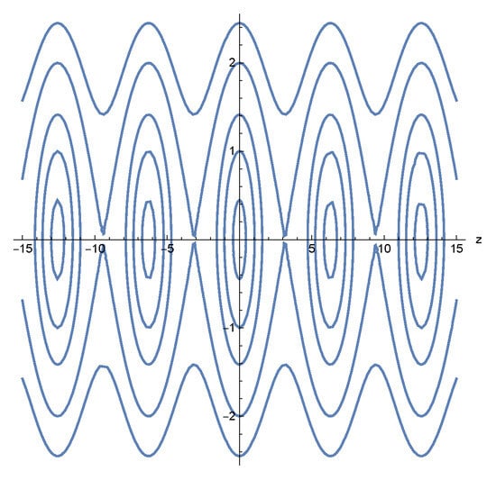
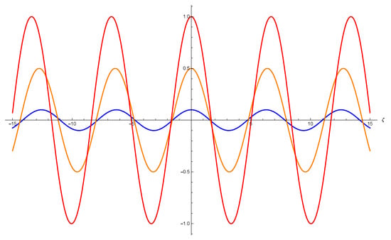
When $c>0,$ we have $J>0$ and $\mathrm{Trace}\left(M_0(0,0)\right)=0,$ which implies the equilibrium point $O_0(0,0)$ is the center point. Using trigonometric identity $sin2k\pi =sin0=0,$ it follows that the equilibrium points $O_{2k}(2k\pi ,0)$ are centers. Similarly, we obtain that the points $O_{2k+1}(2k\pi +\pi ,0)$ are saddles for $c>0$. The phase portrait of system (10) is shown in Figure 1, and we can see that there exists a class of periodic orbits surrounding the infinite number of centers $O_{2k}(2k\pi ,0)$ if $\lambda$ satisfies $\lambda \in (0,{\displaystyle \frac{2}{c}})$. When $c>0$, the numerical simulation of periodic waves of system (10) is plotted in Figure 2.

Figure 1. The phase portrait of system (10) for $c>0$.

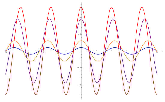
Figure 2. Periodic waves of system (10) for $c>0$.

Since $\sin z$ is the function with a period of $2\pi$ with respect to z, the monotonicity of the period function of periodic solutions surrounding the centers $O_{2k}(2k\pi ,0)$ are the same, we only need to consider the center point $O_0(0,0)$. Let

$$S\left(z\right)=-{\displaystyle \frac{1}{c}}\cos z+{\displaystyle \frac{1}{c}},L\left(z\right)={\displaystyle \frac{S\left(z\right)}{{\left(S^{\prime }\left(z\right)\right)}^2}}={\displaystyle \frac{c}{1+cosz}}.$$

A straightforward computation shows that

$$L^{\prime \prime }\left(z\right)=-{\displaystyle \frac{1}{4}}c(cosz-2){sec}^4\left({\displaystyle \frac{z}{2}}\right)\ge 0$$

holds for all $z\in (-\pi ,\pi ).$ Using Lemma 1, we complete the proof of the first part of Theorem 1.

Next, we consider the asymptotic analysis. Recall that

$${\displaystyle \frac{1}{2}}{y}^2-{\displaystyle \frac{1}{c}}cosz+{\displaystyle \frac{1}{c}}=\lambda$$

(12)

is a first integral of system (10). Let $y=0,$ then Equation (12) yields $z_{1,2}=\pm arccos(1-c\lambda ).$

$$P\left(\lambda \right)=\sqrt{2}{\int }_{z_1}^{z_2}{\displaystyle \frac{\mathrm{d}z}{\sqrt{\lambda +\frac{1}{c}cosz-\frac{1}{c}}}}=\sqrt{2c}{\int }_{-arccos(1-c\lambda )}^{arccos(1-c\lambda )}{\displaystyle \frac{\mathrm{d}z}{\sqrt{c\lambda +cosz-1}}}.$$

(13)

Let

$$z=warccos(1-c\lambda ),$$

(14)

then

$$P\left(\lambda \right)=\sqrt{2c}{\int }_{-1}^1{\displaystyle \frac{arccos(1-c\lambda )}{\sqrt{c\lambda +cos\left(warccos(1-c\lambda )\right)-1}}}\mathrm{d}w.$$

(15)

Let $c\lambda =h.$ Then, we have $h\to 0$ as $\lambda \to 0$. Using the Taylor series in h, we have

$${\displaystyle \frac{arccos(1-c\lambda )}{\sqrt{c\lambda +cos\left(warccos(1-c\lambda )\right)-1}}}={\displaystyle \frac{\sqrt{2}}{\sqrt{1-w^2}}}+{\displaystyle \frac{h\left(\sqrt{2}{w}^2+\sqrt{2}\right)}{12\sqrt{1-w^2}}}+O\left(h^2\right).$$

(16)

Therefore,

$$\underset{\lambda \to 0}{lim}P\left(\lambda \right)=\underset{h\to 0}{lim}\sqrt{2c}{\int }_{-1}^1{\displaystyle \frac{\sqrt{2}}{\sqrt{1-w^2}}}+O\left(h\right)\mathrm{d}w=2\sqrt{c}\pi .$$

Let $arccos(1-c\lambda )=l$, then we obtain $l\to \pi$ as $\lambda \to {\displaystyle \frac{2}{c}}$. Let $lw=q.$ Then, using (15), we have

$$\underset{\lambda \to {\displaystyle \frac{2}{c}}}{lim}P\left(\lambda \right)=\underset{l\to \pi }{lim}\sqrt{2c}{\int }_{-1}^1{\displaystyle \frac{l}{\sqrt{cos\left(wl\right)-cosl}}}\mathrm{d}w=\underset{l\to \pi }{lim}\sqrt{2c}{\int }_{-l}^l{\displaystyle \frac{1}{\sqrt{cosq-cosl}}}\mathrm{d}q=+\infty .$$

This completes the proof of the second part of Theorem 1.

□

When $c=1,$ the graph of the period function $P\left(\lambda \right)$ of system (10) at $\lambda \in (0,2)$ is shown in Figure 3, and it indicates that the numerical result is consistent with the theoretical analysis result.

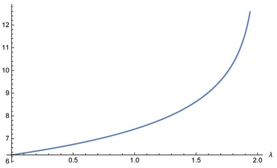
Figure 3. The graph of the period function $P\left(\lambda \right)$ of system (10) for $c=1.$

4. The Monotonicity of the Period Function for the Generalized sG Equation in the Case of $\mathit{a}\ne \mathbf{0}$

In this section, we consider the generalized sG Equation (1) in the case with $a\ne 0$. When $a\cos z+c\ne 0$, using the traveling wave transformation (8), Equation (1) can be written as

$${\displaystyle \frac{\sin z}{a\cos z+c}}-{\left(z^{\prime }\right)}^2{\displaystyle \frac{a\sin z}{a\cos z+c}}+z^{\prime \prime }=0.$$

(17)

Equation (17) is equivalent to the following planar dynamical system:

$$\left\{\begin{array}{c}{\displaystyle \frac{\mathrm{d}z}{\mathrm{d}\zeta }}=y,\hfill \\ {\displaystyle \frac{\mathrm{d}y}{\mathrm{d}\zeta }}={\displaystyle \frac{(a{y}^2-1)sinz}{c+acosz}},\hfill \end{array}\right.$$

(18)

with the first integral

$$H(z,y)=y^2{(c+acosz)}^2-(a{cos}^{2}z+2ccosz-2c-a)=\lambda .$$

(19)

It should be mentioned that system (18) is not a Hamiltonian system but it can be transformed into the form of a Hamiltonian. Note that $z\left(\zeta \right)$ is a solution of (18) if and only if $v\left(\zeta \right)$ is a solution of the following planar Hamiltonian system

$$\left\{\begin{array}{c}{\displaystyle \frac{\mathrm{d}v}{\mathrm{d}\zeta }}=y,\hfill \\ {\displaystyle \frac{\mathrm{d}y}{\mathrm{d}\zeta }}=-W\left(v\right),\hfill \end{array}\right.$$

(20)

where the implicit function $W\left(v\right)={\displaystyle \frac{sinz}{c+a}}$ satisfies the equation

$$cz+asinz=(c+a)v.$$

(21)

Since $W\left(v\right)$ in Hamiltonian system (20) is an implicit function and it cannot be represented explicitly, it is difficult to analyze the monotonicity of the period function using Lemma 1. However, we can tackle this problem using Lemma 2.

Theorem 2.

In the case that $a+c>0$, there are corresponding period annulus surrounding the center points $O_{2k}(2k\pi ,0)$ for Equation (18), where $k\in \mathbb{Z}$.

(1) 

If $c>a>0,$ or in the case that $c>-a>0,$ the corresponding period function $P\left(\lambda \right)$ satisfies $P^{\prime }\left(\lambda \right)\ge 0$ for $0<\lambda <4c$.

(2) 

If $a>c>0,$ then $P^{\prime }\left(\lambda \right)\ge 0$ for $0<\lambda <{\displaystyle \frac{{(a+c)}^2}{a}}$.

(3) 

If $a>-c>0,$ then $P^{\prime }\left(\lambda \right)\le 0$ for $0<\lambda <{\displaystyle \frac{{(a+c)}^2}{a}}$.

Proof. 

Obviously, the points $O_{2k}(2k\pi ,0)$ are equilibria of (18). Since

$$sinz=sin(z+2k\pi ),cosz=cos(z+2k\pi ),$$

from the expression of (18), we only need to consider the point $O_0(0,0)$. Since the linear coefficient matrix of (18) at the origin is

$$\left(\begin{array}{cc}0\hfill & 1\hfill \\ -{\displaystyle \frac{1}{a+c}}\hfill & 0\hfill \end{array}\right),$$

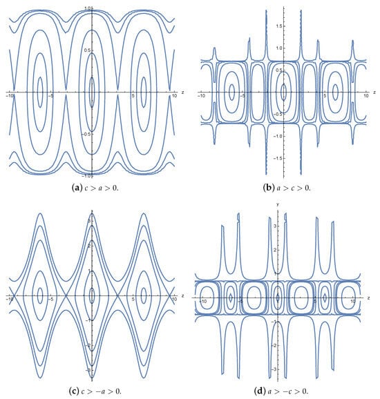
using the theory of planar dynamical system, it follows that the point $O_0(0,0)$ is the center of $a+c>0$. The phase portrait of system (18) is shown in Figure 4 under different parametric conditions.

Figure 4. Phase portraits of system (18) for $a+c>0$.

Using identities

$$sinz=2sin{\displaystyle \frac{z}{2}}cos{\displaystyle \frac{z}{2}},1-{cos}^{2}z={sin}^{2}z,cosz-1=-2{sin}^2{\displaystyle \frac{z}{2}},$$

Equation (19) can be rewritten as

$$H(z,y)=y^2{(c+acosz)}^2+(4a+4c){sin}^2{\displaystyle \frac{z}{2}}-4a{sin}^4{\displaystyle \frac{z}{2}}=\lambda .$$

(22)

When $c>a>0$, or in the case that $c>-a>0,$ there exists a set of period orbits surrounding the center $O_0(0,0)$ for $0<\lambda <4c,$ and the abscissa of the intersection point between the periodic orbit and the z-axis satisfies $-\pi <z<\pi ;$ see Figure 4a,c.

Since systems (18) and (20) have the same monotonicity of the period function defined in the neighborhood of origin, we only consider system (20). Since $W\left(0\right)=0,$ one can set

$$W\left(v\right)=W^{\prime }\left(0\right)v+W_1\left(v\right).$$

(23)

Using polar coordinate transformation $v=rcos\theta$, $y=rsin\theta$, system (20) becomes

$$\left\{\begin{array}{c}{\displaystyle \frac{\mathrm{d}r}{\mathrm{d}\zeta }}=rcos\theta sin\theta -sin\theta W(rcos\theta )=\rho (r,\theta ),\hfill \\ {\displaystyle \frac{\mathrm{d}\theta }{\mathrm{d}\zeta }}=-W^{\prime }\left(0\right){cos}^2\theta -{sin}^2\theta -{\displaystyle \frac{cos\theta W_1(rcos\theta )}{r}}=\omega (r,\theta ).\hfill \end{array}\right.$$

(24)

Note that

$$r^2\omega (r,\theta )=r^2{\displaystyle \frac{\mathrm{d}\theta }{\mathrm{d}\zeta }}=-W^{\prime }\left(0\right)v^2-y^2-v{W}_1\left(v\right)=-vW\left(v\right)-y^2.$$

(25)

Using (21), we obtain

$$vW\left(v\right)=v{\displaystyle \frac{sinz}{c+a}}={\displaystyle \frac{(cz+asinz)sinz}{{(c+a)}^2}}.$$

When $c>a>0$, or in the case that $c>-a>0,$ we obtain that $vW\left(v\right)>0$ for $z\in (-\pi ,0)\cup (0,\pi )$.

Using (25), we have $r^2\omega (r,\theta )<0$ for $z\in (-\pi ,0)\cup (0,\pi ).$ Thus,

$$\begin{array}{cc}\hfill {\displaystyle \frac{\partial \left|\omega \right(r,\theta \left)\right|}{\partial r}}& =-{\displaystyle \frac{\partial \omega (r,\theta )}{\partial r}}=cos\theta {\displaystyle \frac{\partial \left(\frac{W_1(rcos\theta )}{r}\right)}{\partial r}}={\displaystyle \frac{r^2{cos}^2\theta W_1^{\prime }(rcos\theta )-rcos\theta W_1(rcos\theta )}{r^3}}\hfill \\ \hfill & ={\displaystyle \frac{v^2{W}_1^{\prime }\left(v\right)-v{W}_1\left(v\right)}{{(v^2+y^2)}^{\frac{3}{2}}}}\hfill \end{array}$$

(26)

for $\theta \in [0,2\pi )$ and $\theta \ne {\displaystyle \frac{\pi }{2}},{\displaystyle \frac{3\pi }{2}}.$ Using (21) and (23), it can be deduced that

$$W_1^{\prime }\left(v\right)=W^{\prime }\left(v\right)-W^{\prime }\left(0\right)={\displaystyle \frac{cosz}{c+acosz}}-{\displaystyle \frac{1}{c+a}}.$$

(27)

Hence,

$$\begin{array}{cc}\hfill v^2{W}_1^{\prime }\left(v\right)-v{W}_1\left(v\right)& =v^2\left({\displaystyle \frac{cosz}{c+acosz}}-{\displaystyle \frac{1}{c+a}}\right)-v\left({\displaystyle \frac{sinz}{c+a}}-{\displaystyle \frac{1}{c+a}}v\right)\hfill \\ \hfill & =v\left(v{\displaystyle \frac{cosz}{c+acosz}}-{\displaystyle \frac{sinz}{c+a}}\right)\hfill \\ \hfill & ={\displaystyle \frac{c}{{(a+c)}^2}}{\displaystyle \frac{(zcosz-sinz)(asinz+cz)}{acosz+c}}.\hfill \end{array}$$

(28)

When $c>a>0$, or in the case that $c>-a>0,$ we can directly verify that $v^2{W}_1^{\prime }\left(v\right)-v{W}_1\left(v\right)<0$ for $z\in (-\pi ,0)\cup (0,\pi ).$ Using (26), we obtain ${\displaystyle \frac{\partial \left|\omega \right(r,\theta \left)\right|}{\partial r}}\le 0$ for almost all $\theta \in [0,2\pi )$. From Lemma 2, we have $P^{\prime }\left(\lambda \right)\ge 0$ for $0<\lambda <4c$.

Similarly, when $a>c>0,$ we have $v^2{W}_1^{\prime }\left(v\right)-v{W}_1\left(v\right)<0$ for $z\in (-arccos(-{\displaystyle \frac{c}{a}}),0)\cup (0,arccos(-{\displaystyle \frac{c}{a}}))$. Using (26) again, we obtain ${\displaystyle \frac{\partial \left|\omega \right(r,\theta \left)\right|}{\partial r}}\le 0$ for $z\in (-arccos(-{\displaystyle \frac{c}{a}}),0)\cup (0,arccos(-{\displaystyle \frac{c}{a}}))$. From Lemma 2, we have $P^{\prime }\left(\lambda \right)\ge 0$ for $0<\lambda <{\displaystyle \frac{{(a+c)}^2}{a}}$.

When $a>-c>0$, we have $v^2{W}_1^{\prime }\left(v\right)-v{W}_1\left(v\right)>0$ for $z\in (-arccos(-{\displaystyle \frac{c}{a}}),0)\cup (0,arccos(-{\displaystyle \frac{c}{a}}))$. Using (26), it yields ${\displaystyle \frac{\partial \left|\omega \right(r,\theta \left)\right|}{\partial r}}\ge 0$ for $z\in (-arccos(-{\displaystyle \frac{c}{a}}),0)\cup (0,arccos(-{\displaystyle \frac{c}{a}}))$. From Lemma 2, we obtain $P^{\prime }\left(\lambda \right)\le 0$ for $0<\lambda <{\displaystyle \frac{{(a+c)}^2}{a}}$.

□

Taking $c=2$ and $a=1,$ the plot of $P\left(\lambda \right)$ for $\lambda \in (0,4c)$ is presented in Figure 5a. Taking $c=2$ and $a=-1,$ the plot of $P\left(\lambda \right)$ for $\lambda \in (0,4c)$ is shown in Figure 5b. Taking $a=2$ and $c=1,$ the plot of $P\left(\lambda \right)$ for $\lambda \in (0,{\displaystyle \frac{{(a+c)}^2}{a}})$ is presented in Figure 5c. Taking $a=2$ and $c=-1,$ the plot of $P\left(\lambda \right)$ for $\lambda \in (0,{\displaystyle \frac{{(a+c)}^2}{a}})$ is shown in Figure 5d. The numerical simulation verifies the qualitative analytical results of Theorem 2.

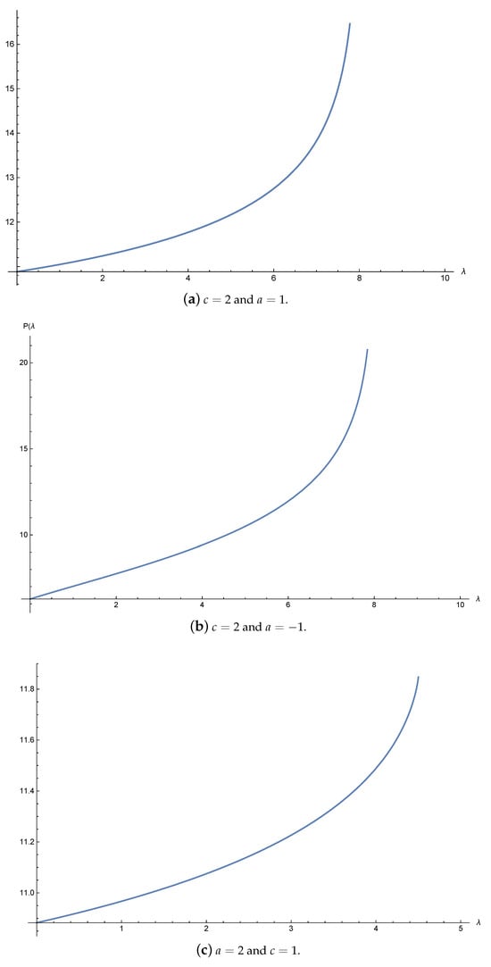
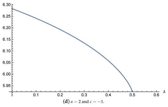
Figure 5. When $a+c>0$, the plots of $P\left(\lambda \right)$ are associated with the center $O_0(0,0)$ for system (18).

Theorem 3.

In the case that $a>-c>0$, there are corresponding period annulus surrounding the center points $O_{2k+1}(2k\pi +\pi ,0)$ for Equation (18), where $k\in \mathbb{Z}$. The corresponding period function $P\left(\lambda \right)$ satisfies $P^{\prime }\left(\lambda \right)\ge 0$ for $4c<\lambda <{\displaystyle \frac{{(a-c)}^2}{a}}$.

Proof. 

It is straightforward to verify that the points $O_{2k+1}(2k\pi +\pi ,0)$ are equilibria of (18). We make a translation to move the equilibrium points $O_{2k+1}(2k\pi +\pi ,0)$ to the origin. Let $z-(2k\pi +\pi )=\widehat{z}$ and $y-0=\widehat{y}$. Then, system (18) becomes

$$\left\{\begin{array}{c}{\displaystyle \frac{\mathrm{d}\widehat{z}}{\mathrm{d}\zeta }}=\widehat{y},\hfill \\ {\displaystyle \frac{\mathrm{d}\widehat{y}}{\mathrm{d}\zeta }}={\displaystyle \frac{(1-a{\widehat{y}}^2)sin\widehat{z}}{c-acos\widehat{z}}}.\hfill \end{array}\right.$$

(29)

The linear coefficient matrix of (29) at the origin is as follows:

$$\left(\begin{array}{cc}0\hfill & 1\hfill \\ {\displaystyle \frac{1}{c-a}}\hfill & 0\hfill \end{array}\right).$$

Using the theory of the planar dynamical system, it follows that the points $O_{2k+1}(2k\pi +\pi ,0)$ are centers for $a>-c>0$. From Figure 4d, we can see that there are corresponding period annulus surrounding the center points $O_{2k+1}(2k\pi +\pi ,0)$ for Equation (18).

Note that $\widehat{z}\left(\zeta \right)$ is a solution of (29) if and only if $\widehat{v}\left(\zeta \right)$ is a solution of the planar Hamiltonian system:

$$\left\{\begin{array}{c}{\displaystyle \frac{\mathrm{d}\widehat{v}}{\mathrm{d}\zeta }}=\widehat{y},\hfill \\ {\displaystyle \frac{\mathrm{d}\widehat{y}}{\mathrm{d}\zeta }}=-\widehat{W}\left(\widehat{v}\right),\hfill \end{array}\right.$$

(30)

where the implicit function $\widehat{W}\left(\widehat{v}\right)={\displaystyle \frac{sin\widehat{z}}{a-c}}$ satisfies the following equation:

$$-c\widehat{z}+asin\widehat{z}=(a-c)\widehat{v}.$$

(31)

Since $\widehat{W}\left(0\right)=0,$ we set

$$\widehat{W}\left(\widehat{v}\right)={\widehat{W}}^{\prime }\left(0\right)\widehat{v}+{\widehat{W}}_1\left(\widehat{v}\right).$$

(32)

Let $\widehat{v}=\widehat{r}cos\widehat{\theta }$, $y=\widehat{r}sin\widehat{\theta }$. Then, system (30) becomes

$$\left\{\begin{array}{c}{\displaystyle \frac{\mathrm{d}\widehat{r}}{\mathrm{d}\zeta }}=\widehat{r}cos\widehat{\theta }sin\widehat{\theta }-sin\widehat{\theta }\widehat{W}(\widehat{r}cos\widehat{\theta })=\widehat{\rho }(\widehat{r},\widehat{\theta }),\hfill \\ {\displaystyle \frac{\mathrm{d}\widehat{\theta }}{\mathrm{d}\zeta }}=-{\widehat{W}}^{\prime }\left(0\right){cos}^2\widehat{\theta }-{sin}^2\widehat{\theta }-{\displaystyle \frac{cos\widehat{\theta }{\widehat{W}}_1(\widehat{r}cos\widehat{\theta })}{\widehat{r}}}=\widehat{\omega }(\widehat{r},\widehat{\theta }).\hfill \end{array}\right.$$

(33)

Obviously,

$${\widehat{r}}^2\widehat{\omega }(\widehat{r},\widehat{\theta })={\widehat{r}}^2{\displaystyle \frac{\mathrm{d}\widehat{\theta }}{\mathrm{d}\zeta }}=-\widehat{v}\widehat{W}\left(\widehat{v}\right)-{\widehat{y}}^2.$$

(34)

Using (31), we obtain

$$\widehat{v}\widehat{W}\left(\widehat{v}\right)=\widehat{v}{\displaystyle \frac{sin\widehat{z}}{a-c}}={\displaystyle \frac{(-c\widehat{z}+asin\widehat{z})sin\widehat{z}}{{(a-c)}^2}}.$$

When $a>-c>0$, we obtain that $\widehat{v}\widehat{W}\left(\widehat{v}\right)>0$ for $\widehat{z}\in (-\pi ,0)\cup (0,\pi ).$ Using (34), we have ${\widehat{r}}^2\widehat{\omega }(\widehat{r},\widehat{\theta })<0$ for $\widehat{z}\in (-\pi ,0)\cup (0,\pi ).$ Thus,

$${\displaystyle \frac{\partial |\widehat{\omega }(\widehat{r},\widehat{\theta })|}{\partial \widehat{r}}}=-{\displaystyle \frac{\partial \widehat{\omega }(\widehat{r},\widehat{\theta })}{\partial \widehat{r}}}={\displaystyle \frac{{\widehat{v}}^2{\widehat{W}}_1^{\prime }\left(\widehat{v}\right)-\widehat{v}{\widehat{W}}_1\left(\widehat{v}\right)}{{({\widehat{v}}^2+{\widehat{y}}^2)}^{\frac{3}{2}}}}$$

(35)

for $\widehat{z}\in (-\pi ,0)\cup (0,\pi ).$ Using (31), we have

$${\widehat{W}}_1^{\prime }\left(\widehat{v}\right)={\widehat{W}}^{\prime }\left(\widehat{v}\right)-{\widehat{W}}^{\prime }\left(0\right)={\displaystyle \frac{cos\widehat{z}}{-c+acos\widehat{z}}}-{\displaystyle \frac{1}{a-c}}.$$

(36)

Therefore,

$${\widehat{v}}^2{\widehat{W}}_1^{\prime }\left(\widehat{v}\right)-\widehat{v}{\widehat{W}}_1\left(\widehat{v}\right)={\displaystyle \frac{-c}{{(a-c)}^2}}{\displaystyle \frac{(\widehat{z}cos\widehat{z}-sin\widehat{z})(asin\widehat{z}-c\widehat{z})}{acos\widehat{z}-c}}.$$

(37)

When $a>-c>0$, we can verify that ${\widehat{v}}^2{\widehat{W}}_1^{\prime }\left(\widehat{v}\right)-\widehat{v}{\widehat{W}}_1\left(\widehat{v}\right)<0$ for $\widehat{z}\in (-arccos(-{\displaystyle \frac{c}{a}}),0)\cup (0,arccos(-{\displaystyle \frac{c}{a}}))$. Using (35), we obtain ${\displaystyle \frac{\partial |\widehat{\omega }(\widehat{r},\widehat{\theta })|}{\partial \widehat{r}}}<0$ for $\widehat{z}\in (-arccos(-{\displaystyle \frac{c}{a}}),0)\cup (0,arccos(-{\displaystyle \frac{c}{a}}))$. Returning to Equations (18) and (19), using Lemma 2, we have $P^{\prime }\left(\lambda \right)\ge 0$ for $4c<\lambda <{\displaystyle \frac{{(a-c)}^2}{a}}$.

□

Taking $a=2$ and $c=-1,$ the plot of $P\left(\lambda \right)$ for $\lambda \in (4c,{\displaystyle \frac{{(a-c)}^2}{a}})$ is presented in Figure 6. The numerical simulation verifies the qualitative analytical results of Theorem 3.

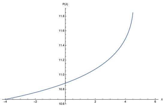
Figure 6. When $a=2$ and $c=-1,$ the plot of $P\left(\lambda \right)$ associated with the center $O_1(\pi ,0)$ for system (18).

5. The Monotonicity of the Period Function for the sP Equation

Let

$$\xi =k_{1}x+k_{2}y,$$

(38)

where $k_1$ and $k_2$ are constants. Substituting (38) into Equation (2) yields

$$k_1^2{\displaystyle \frac{{\mathrm{d}}^{2}u}{\mathrm{d}{\xi }^2}}+k_2^2{\displaystyle \frac{{\mathrm{d}}^{2}u}{\mathrm{d}{\xi }^2}}=-\sigma {\displaystyle \frac{{\mathrm{e}}^u-{\mathrm{e}}^{-u}}{2}}.$$

(39)

Equation (39) can be written as a plane Hamiltonian system:

$$\left\{\begin{array}{c}{\displaystyle \frac{\mathrm{d}u}{\mathrm{d}\xi }}=p,\hfill \\ {\displaystyle \frac{\mathrm{d}p}{\mathrm{d}\xi }}=-N\left(u\right),\hfill \end{array}\right.$$

(40)

with Hamiltonian

$$H(u,p)={\displaystyle \frac{1}{2}}{p}^2-{\displaystyle \frac{b}{2}}({\mathrm{e}}^u+{\mathrm{e}}^{-u})+b=\lambda ,$$

(41)

where $N\left(u\right)=-b{\displaystyle \frac{{\mathrm{e}}^u-{\mathrm{e}}^{-u}}{2}}$, $b=-{\displaystyle \frac{\sigma }{k_1^2+k_2^2}}$, and $k_1^2+k_2^2\ne 0.$ Since $\sigma >0,$ we have $b<0$.

Theorem 4.

In the case that $b<0$, there is a class of periodic solutions in a neighborhood of the point $O(0,0)$ for Equation (40). The period function satisfies $P^{\prime }\left(\lambda \right)\le 0$ for $\lambda \in (0,+\infty )$. Moreover, $\underset{\lambda \to 0}{lim}P\left(\lambda \right)={\displaystyle \frac{2\pi }{\sqrt{-b}}}$ and $\underset{\lambda \to +\infty }{lim}P\left(\lambda \right)=0.$

Proof. 

When $b\ne 0$, there is an equilibrium point $O(0,0)$ of system (40). Since the linear coefficient matrix of (40) at equilibrium point $O(0,0)$ is

$$\left(\begin{array}{cc}0\hfill & 1\hfill \\ b\hfill & 0\hfill \end{array}\right),$$

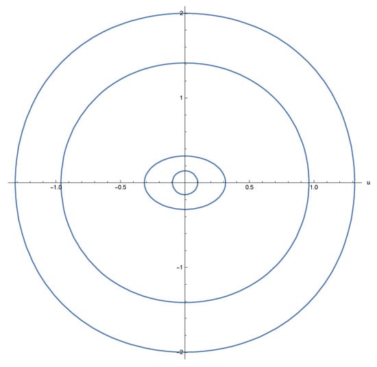
by the theory of the planar dynamical system, we know that the equilibrium point $O(0,0)$ is a center point for $b<0$. With numerical simulations, the phase portrait of system (40) is plotted in Figure 7, and the periodic waves are plotted in Figure 8.

Figure 7. Phase portrait of (40) for $b<0$.

Figure 8. Periodic waves of (40) for $b<0$.

From Figure 7, we can see that if $b<0$ and $\lambda >0$, then there is a class of periodic orbits in a neighborhood of the center $O(0,0)$. Using (41), we have

$$P\left(\lambda \right)={\oint }_{{{\rm Y}}_{\lambda }}{\displaystyle \frac{\mathrm{d}u}{p}}=\sqrt{2}{\int }_{u_1}^{u_2}{\displaystyle \frac{\mathrm{d}u}{\sqrt{\lambda +\frac{b}{2}({\mathrm{e}}^u+{\mathrm{e}}^{-u})-b}}},$$

(42)

where $u_1$ and $u_2$ are the roots of equation $-{\displaystyle \frac{b}{2}}({\mathrm{e}}^u+{\mathrm{e}}^{-u})+b=\lambda$, and $u_1<0<u_2.$ Since $H(u,p)$ is an even function with respect to u and p, it yields that $u_1=-u_2$.

Since $N\left(0\right)=0,$ we set

$$N\left(u\right)=N^{\prime }\left(0\right)u+N_1\left(u\right).$$

(43)

Using the polar coordinate transformation $u=\tilde{r}cos\tilde{\theta }$, $p=\tilde{r}sin\tilde{\theta }$, system (40) becomes

$$\left\{\begin{array}{c}{\displaystyle \frac{\mathrm{d}\tilde{r}}{\mathrm{d}\xi }}=\tilde{r}cos\tilde{\theta }sin\tilde{\theta }-sin\tilde{\theta }N(\tilde{r}cos\tilde{\theta })=\tilde{\rho }(\tilde{r},\tilde{\theta }),\hfill \\ {\displaystyle \frac{\mathrm{d}\tilde{\theta }}{\mathrm{d}\xi }}=-N^{\prime }\left(0\right){cos}^2\tilde{\theta }-{sin}^2\tilde{\theta }-{\displaystyle \frac{cos\tilde{\theta }{N}_1(\tilde{r}cos\tilde{\theta })}{\tilde{r}}}=\tilde{\omega }(\tilde{r},\tilde{\theta }).\hfill \end{array}\right.$$

(44)

Note that

$${\tilde{r}}^2\tilde{\omega }(\tilde{r},\tilde{\theta })={\tilde{r}}^2{\displaystyle \frac{\mathrm{d}\tilde{\theta }}{\mathrm{d}\xi }}=-N^{\prime }\left(0\right)u^2-p^2-u{N}_1\left(u\right)=-uN\left(u\right)-p^2.$$

(45)

When $b<0,$ we have

$$uN\left(u\right)=-bu{\displaystyle \frac{{\mathrm{e}}^u-{\mathrm{e}}^{-u}}{2}}>0$$

for $u\in \mathbb{R}\setminus \left\{0\right\}$. Using (45), we obtain ${\tilde{r}}^2\tilde{\omega }(\tilde{r},\tilde{\theta })<0$ for $u\in \mathbb{R}\setminus \left\{0\right\}$.

Thus,

$${\displaystyle \frac{\partial |\tilde{\omega }(\tilde{r},\tilde{\theta })|}{\partial \tilde{r}}}=-{\displaystyle \frac{\partial \tilde{\omega }(\tilde{r},\tilde{\theta })}{\partial \tilde{r}}}=cos\tilde{\theta }{\displaystyle \frac{\partial \left(\frac{N_1(\tilde{r}cos\tilde{\theta })}{\tilde{r}}\right)}{\partial \tilde{r}}}={\displaystyle \frac{u^2{N}_1^{\prime }\left(u\right)-u{N}_1\left(u\right)}{{(u^2+p^2)}^{\frac{3}{2}}}}$$

(46)

for $\tilde{\theta }\in [0,2\pi )$ and $\tilde{\theta }\ne {\displaystyle \frac{\pi }{2}},{\displaystyle \frac{3\pi }{2}}.$ Obviously,

$$N_1^{\prime }\left(u\right)=N^{\prime }\left(u\right)-N^{\prime }\left(0\right)=-b{\displaystyle \frac{{\mathrm{e}}^u+{\mathrm{e}}^{-u}}{2}}+b.$$

(47)

Thus,

$$\begin{array}{cc}\hfill u^2{N}_1^{\prime }\left(u\right)-u{N}_1\left(u\right)& =u^2\left(-b{\displaystyle \frac{{\mathrm{e}}^u+{\mathrm{e}}^{-u}}{2}}+b\right)-u\left(-b{\displaystyle \frac{{\mathrm{e}}^u-{\mathrm{e}}^{-u}}{2}}+bu\right)\hfill \\ \hfill & =bu\left(sinhu-ucoshu\right).\hfill \end{array}$$

(48)

When $b<0$, we have $u^2{N}_1^{\prime }\left(u\right)-u{N}_1\left(u\right)>0$ for $u\in \mathbb{R}\setminus \left\{0\right\}$. Using (46), we obtain ${\displaystyle \frac{\partial |\tilde{\omega }(\tilde{r},\tilde{\theta })|}{\partial \tilde{r}}}\ge 0$ for $\tilde{\theta }\in [0,2\pi )$ and $\tilde{\theta }\ne {\displaystyle \frac{\pi }{2}},{\displaystyle \frac{3\pi }{2}}.$ From Lemma 2, we have $P^{\prime }\left(\lambda \right)\le 0$ for $\lambda \in (0,+\infty )$.

Next, we discuss the asymptotic behavior of $P\left(\lambda \right)$. Recall that

$$P\left(\lambda \right)=\sqrt{2}{\int }_{u_1}^{u_2}{\displaystyle \frac{\mathrm{d}u}{\sqrt{\lambda +\frac{b}{2}({\mathrm{e}}^u+{\mathrm{e}}^{-u})-b}}}$$

(49)

and $u_1=-u_2.$ Since $u_1$ and $u_2$ are the roots of equation

$$-{\displaystyle \frac{b}{2}}({\mathrm{e}}^u+{\mathrm{e}}^{-u})+b=\lambda$$

(50)

and $u_1$=$-u_2$, it deduces that $\underset{\lambda \to 0}{lim}{u}_1=0=\underset{\lambda \to 0}{lim}{u}_2.$ Let

$$u=u_{2}w.$$

Then, Equation (49) becomes

$$P\left(\lambda \right)=\sqrt{2}{\int }_{-1}^1{\displaystyle \frac{u_2\mathrm{d}w}{\sqrt{\lambda +\frac{b}{2}({\mathrm{e}}^{w{u}_2}+{\mathrm{e}}^{-w{u}_2})-b}}}.$$

(51)

Using (50) and the Taylor expansion with respect to $u_2$, we have

$${\displaystyle \frac{u_2}{\sqrt{\lambda +\frac{b}{2}({\mathrm{e}}^{w{u}_2}+{\mathrm{e}}^{-w{u}_2})-b}}}={\displaystyle \frac{\sqrt{2}}{\sqrt{-b\left(1-w^2\right)}}}-{\displaystyle \frac{u_2^2\left(w^2+1\right)}{12\left(\sqrt{2}\sqrt{-b\left(1-w^2\right)}\right)}}+O\left(u_2^2\right).$$

(52)

Thus, using (51) and (52), we obtain

$$\underset{u_2\to 0}{lim}P=\sqrt{2}{\int }_{-1}^1{\displaystyle \frac{\sqrt{2}\mathrm{d}w}{\sqrt{-b(1-w^2)}}}={\displaystyle \frac{2}{\sqrt{-b}}}\pi .$$

(53)

It follows that $P\to {\displaystyle \frac{2}{\sqrt{-b}}}\pi$ as $\lambda \to 0.$

We also can obtain that $\underset{\lambda \to +\infty }{lim}P\left(\lambda \right)=0.$ The proof process of the asymptotic property of $\lambda \to +\infty$ is similar to that of $\lambda \to 0$, so we omit it here. □

Taking $b=-2,$ the plot of $P\left(\lambda \right)$ for $\lambda \in (0,-b)$ is presented in Figure 9a, and the plot of $P\left(\lambda \right)$ for $\lambda \in (-b,-100b)$ is presented in Figure 9b, the plot of $P\left(\lambda \right)$ at infinity is also presented in Figure 9c. The numerical simulation verifies the qualitative analytical results of Theorem 4.

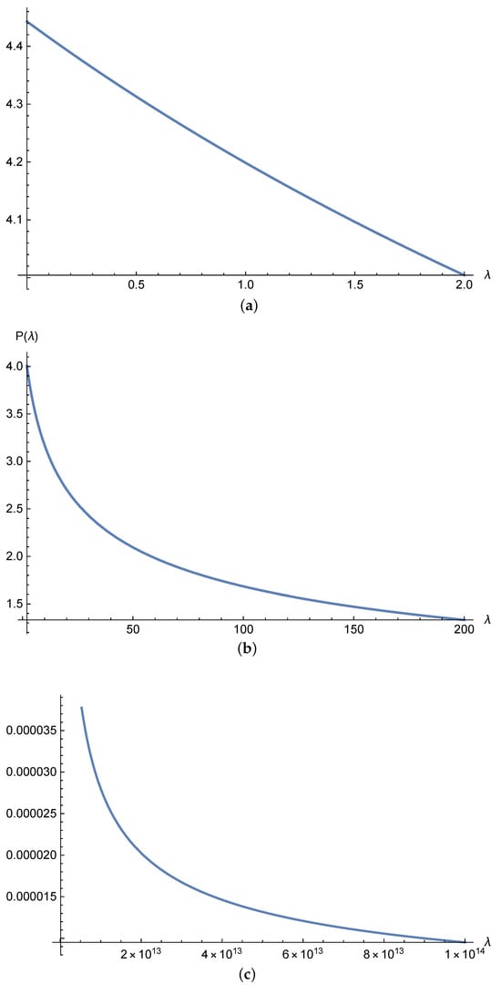
Figure 9. The plots of $P\left(\lambda \right)$ at $b=-2.$

Remark 2.

If Lemma 1 is used to analyze the monotonicity of the period function (42), then we can only obtain that $P^{\prime }\left(\lambda \right)\le 0$ for $\lambda \in (0,-b)$, but the monotonicity of $P\left(\lambda \right)$ on $(-b,+\infty )$ cannot be theoretically proven directly. In fact, choosing $S\left(u\right)=-{\displaystyle \frac{b}{2}}({\mathrm{e}}^u+{\mathrm{e}}^{-u})+b$, we have

$$L\left(u\right)={\displaystyle \frac{S\left(u\right)}{{\left(S^{\prime }\left(u\right)\right)}^2}}={\displaystyle \frac{-2({\mathrm{e}}^u+{\mathrm{e}}^{-u})+4}{b{({\mathrm{e}}^u-{\mathrm{e}}^{-u})}^2}}.$$

(54)

Taking the derivative of $L\left(u\right)$ twice, it yields

$$L^{\prime \prime }\left(u\right)={\displaystyle \frac{2{\mathrm{e}}^u\left({\mathrm{e}}^{2u}-4{\mathrm{e}}^u+1\right)}{-b{\left({\mathrm{e}}^u+1\right)}^4}}.$$

(55)

A short calculation revealed that for $u\in (-ln(2+\sqrt{3}),ln(2+\sqrt{3}))$, $L^{″}\left(u\right)<0$ holds. From Lemma 1, it implies that $P^{\prime }\left(\lambda \right)\le 0$ for $\lambda \in (0,-b)$. However, Equation (55) yields that $L^{″}\left(u\right)>0$ for $u>ln(2+\sqrt{3}).$ Thus, $L^{″}\left(u\right)<0$ is impossible for all $u\in (ln(2+\sqrt{3}),+\infty )$, and the condition of Lemma 1 is not satisfied.

6. Conclusions

In this paper, we considered the monotonicity of the period function of the generalized sine-Gordon Equation (1) and the sinh-Poisson Equation (2). Using Lemma 1, we obtained the monotonicity of the period function of Equation (1) for $a=0$, and the result can be found in Theorem 1. Using Lemma 2, we obtained the monotonicity of the period function of Equation (1) for $a\ne 0$, and the results can be found in Theorems 2 and 3. Using Lemma 2, the monotonicity of the period function of Equation (2) was provided, and the result can be found in Theorem 4. The numerical simulations were used, and the results of the numerical simulations were consistent with the theoretical analysis. In the future, we will further investigate the stability of the periodic solutions of Equations (1) and (2).

References

- Bastianello, A. Sine-Gordon model from coupled condensates: A generalized hydrodynamics viewpoint. Phys. Rev. B 2024, 109, 35118. [Google Scholar] [CrossRef]
- De Santis, D.; Guarcello, C.; Spagnolo, B.; Carollo, A.; Valenti, D. Breather dynamics in a stochastic sine-Gordon equation: Evidence of noise-enhanced stability. Chaos Soliton. Fract. 2023, 168, 113115. [Google Scholar] [CrossRef]
- Rezazadeh, H.; Zabihi, A.; Davodi, A.G.; Ansari, R.; Ahmad, H.; Yao, S.W. New optical solitons of double sine-Gordon equation using exact solutions methods. Results Phys. 2023, 49, 106452. [Google Scholar] [CrossRef]
- Guo, J.; Li, M. The dynamics of some exact solutions to a (3+1)-dimensional sine-Gordon equation. Wave Motion. 2024, 130, 103354. [Google Scholar] [CrossRef]
- Dauxois, T.; Fauve, S.; Tuckerman, L. Stability of periodic arrays of vortices. Phys. Fluids. 1996, 8, 487–495. [Google Scholar] [CrossRef]
- Zaslavsky, G.M.; Sagdeev, R.Z.; Usikov, D.A. Weak Chaos and Quasi-Regular Patterns; Cambridge University Press: New York, NY, USA, 1992. [Google Scholar]
- Fokas, A.S. On a class of physically important integrable equations. Phys. D 1995, 87, 145–150. [Google Scholar] [CrossRef]
- Ling, L.; Sun, X. On the elliptic-localized solutions of the sine-Gordon equation. Phys. D. 2023, 444, 133597. [Google Scholar] [CrossRef]
- Lenells, J.; Fokas, A.S. On a novel integrable generalization of the sine-Gordon equation. J. Math. Phys. 2010, 51, 23519. [Google Scholar] [CrossRef]
- Matsuno, Y. A direct method for solving the generalized sine-Gordon equation. J. Phys. A-Math. Theor. 2010, 43, 105204. [Google Scholar] [CrossRef]
- Matsuno, Y. A direct method for solving the generalized sine-Gordon equation II. J. Phys. A-Math. Theor. 2010, 43, 375201. [Google Scholar] [CrossRef]
- Gatlik, J.; Dobrowolski, T.; Kevrekidis, P.G. Kink-inhomogeneity interaction in the sine-Gordon model. Phys. Rev. E 2023, 108, 34203. [Google Scholar] [CrossRef] [PubMed]
- Carretero-González, R.; Cisneros-Ake, L.A.; Decker, R.; Koutsokostas, G.N.; Frantzeskakis, D.J.; Kevrekidis, P.G.; Ratliff, D.J. Kink-antikink stripe interactions in the two-dimensional sine-Gordon equation. Commun. Nonlinear Sci. 2022, 109, 106123. [Google Scholar] [CrossRef]
- Feng, B.F.; Sheng, H.H.; Yu, G.F. Integrable semi-discretizations and self-adaptive moving mesh method for a generalized sine-Gordon equation. Numer. Algorithms 2023, 94, 351–370. [Google Scholar] [CrossRef]
- Sheng, H.H.; Feng, B.F.; Yu, G.F. A generalized sine-Gordon equation: Reductions and integrable discretizations. J. Nonlinear Sci. 2024, 34, 55. [Google Scholar] [CrossRef]
- Xiang, X.; Zhao, S.; Shi, Y. Solutions and continuum limits to nonlocal discrete sine-Gordon equations: Bilinearization reduction method. Stud. Appl. Math. 2023, 150, 1274–1303. [Google Scholar] [CrossRef]
- Lührmann, J.; Schlag, W. Asymptotic stability of the sine-Gordon kink under odd perturbations. Duke Math. J. 2023, 172, 2715–2820. [Google Scholar] [CrossRef]
- Montgomery, D.; Matthaeus, W.H.; Stribling, W.T.; Martinez, D.; Oughton, S. Relaxation in two dimensions and the “sinh-Poisson" equation. Phys. Fluids A Fluid Dyn. 1992, 4, 3–6. [Google Scholar] [CrossRef]
- Ting, A.C.; Chen, H.H.; Lee, Y.C. Exact solutions of a nonlinear boundary value problem: The vortices of the two-dimensional sinh-Poisson equation. Phys. D 1987, 26, 37–66. [Google Scholar] [CrossRef]
- Gurarie, D.; Chow, K.W. Vortex arrays for sinh-Poisson equation of two-dimensional fluids: Equilibria and stability. Phys. Fluids 2004, 16, 3296–3305. [Google Scholar] [CrossRef]
- Bartsch, T.; Pistoia, A.; Weth, T. N-vortex equilibria for ideal fluids in bounded planar domains and new nodal solutions of the sinh-Poisson and the Lane-Emden-Fowler equations. Commun. Math. Phys. 2010, 297, 653–686. [Google Scholar] [CrossRef]
- Grossi, M.; Pistoia, A. Multiple blow-up phenomena for the sinh-Poisson equation. Arch. Ration. Mech. Anal. 2013, 209, 287–320. [Google Scholar] [CrossRef]
- McDonald, B.E. Numerical calculation of nonunique solutions of a two-dimensional sinh-Poisson equation. J. Comput. Phys. 1974, 16, 360–370. [Google Scholar] [CrossRef]
- DelaTorre, A.; Mancini, G.; Pistoia, A. Sign-changing solutions for the one-dimensional non-local sinh-Poisson equation. Adv. Nonlinear Stud. 2020, 20, 739–767. [Google Scholar] [CrossRef]
- Figueroa, P. Sign-changing bubble tower solutions for sinh-Poisson type equations on pierced domains. J. Differ. Equ. 2023, 367, 494–548. [Google Scholar] [CrossRef]
- Bartolucci, D.; Pistoia, A. Existence and qualitative properties of concentrating solutions for the sinh-Poisson equation. IMA J. Appl. Math. 2007, 72, 706–729. [Google Scholar] [CrossRef]
- Li, J.; Qiao, Z. Bifurcation and traveling wave solutions for the Fokas equation. Int. J. Bifurcat. Chaos. 2015, 25, 1550136. [Google Scholar] [CrossRef]
- Zhang, Z.A.; Lou, S.Y. Linear superposition for a sine-Gordon equation with some types of novel nonlocalities. Phys. Scr. 2023, 98, 35211. [Google Scholar] [CrossRef]
- Novkoski, F.; Falcon, E.; Pham, C.T. A numerical direct scattering method for the periodic sine-Gordon equation. Eur. Phys. J. Plus. 2023, 138, 1146. [Google Scholar] [CrossRef]
- Chow, K.W.; Mak, C.C.; Rogers, C.; Schief, W.K. Doubly periodic and multiple pole solutions of the sinh-Poisson equation: Application of reciprocal transformations in subsonic gas dynamics. J. Comput. Appl. Math. 2006, 190, 114–126. [Google Scholar] [CrossRef][Green Version]
- Chow, K.W.; Tsang, S.C.; Mak, C.C. Another exact solution for two-dimensional, inviscid sinh-Poisson vortex arrays. Phys. Fluids 2003, 15, 2437–2440. [Google Scholar] [CrossRef]
- Zhang, X.; Boyd, J.P. Exact solutions to a nonlinear partial differential equation: The product-of-curvatures Poisson (uxxuyy = 1). J. Comput. Appl. Math. 2022, 406, 113866. [Google Scholar] [CrossRef]
- Tracy, E.R.; Chin, C.H.; Chen, H.H. Real periodic solutions of the Liouville equation. Phys. D 1986, 23, 91–101. [Google Scholar] [CrossRef]
- Wang, S.; Zhou, Z. Periodic solutions for a second-order partial difference equation. J. Appl. Math. Comput. 2023, 69, 731–752. [Google Scholar] [CrossRef]
- Geyer, A.; Martins, R.H.; Natali, F.; Pelinovsky, D.E. Stability of smooth periodic travelling waves in the Camassa-Holm equation. Stud. Appl. Math. 2022, 148, 27–61. [Google Scholar] [CrossRef]
- Johnson, M.A.; Noble, P.; Rodrigues, L.M.; Zumbrun, K. Behavior of periodic solutions of viscous conservation laws under localized and nonlocalized perturbations. Invent. Math. 2014, 197, 115–213. [Google Scholar] [CrossRef]
- Hakkaev, S.; Stanislavova, M.; Stefanov, A. Spectral stability for classical periodic waves of the Ostrovsky and short pulse models. Stud. Appl. Math. 2017, 139, 405–433. [Google Scholar] [CrossRef]
- Pava, J.A.; Bona, J.L.; Scialom, M. Stability of cnoidal waves. Adv. Differential Equ. 2006, 11, 1321–1374. [Google Scholar]
- Chen, X.; Wang, Z.; Zhang, W. Reachability of maximal number of critical periods without independence. J. Differ. Equ. 2020, 269, 9783–9803. [Google Scholar] [CrossRef]
- Li, C.; Lu, K. The period function of hyperelliptic Hamiltonian of degree 5 with real critical points. Nonlinearity 2008, 21, 465–483. [Google Scholar] [CrossRef]
- Wang, Q.; Huang, W. Limit periodic travelling wave solution of a model for biological invasions. Appl. Math. Lett. 2014, 34, 13–16. [Google Scholar] [CrossRef]
- Chen, A.; Tian, C.; Huang, W. Periodic solutions with equal period for the Friedmann-Robertson-Walker model. Appl. Math. Lett. 2018, 77, 101–107. [Google Scholar] [CrossRef]
- Chen, A.; Guo, L.; Deng, X. Existence of solitary waves and periodic waves for a perturbed generalized BBM equation. J. Differ. Equ. 2016, 261, 5324–5349. [Google Scholar] [CrossRef]
- Chen, A.; Li, J.; Huang, W. The monotonicity and critical periods of periodic waves of the ϕ6 field model. Nonlinear Dynam. 2011, 63, 205–215. [Google Scholar] [CrossRef]
- Lu, L.; He, X.; Chen, A. Bifurcations analysis and monotonicity of the period function of the Lakshmanan-Porsezian-Daniel equation with Kerr Law of nonlinearity. Qual. Theor. Dyn. Syst. 2024, 23, 179. [Google Scholar] [CrossRef]
- Chen, A.; Zhang, C.; Huang, W. Monotonicity of limit wave speed of traveling wave solutions for a perturbed generalized KdV equation. Appl. Math. Lett. 2021, 121, 107381. [Google Scholar] [CrossRef]
- Sun, X.; Yu, P. Periodic traveling waves in a generalized BBM equation with weak backward diffusion and dissipation terms. Discrete Cont. Dyn.-B 2019, 24, 965–987. [Google Scholar] [CrossRef]
- Chicone, C. The monotonicity of the period function for planar Hamiltonian vector fields. J. Differ. Equ. 1987, 69, 310–321. [Google Scholar] [CrossRef]
- Sabatini, M. On the period function of Liénard systems. J. Differ. Equ. 1999, 152, 467–487. [Google Scholar] [CrossRef]
- Chow, S.N.; Hale, J.K. Method of Bifurcation Theory; Springer: New York, NY, USA, 1981. [Google Scholar]
Disclaimer/Publisher’s Note: The statements, opinions and data contained in all publications are solely those of the individual author(s) and contributor(s) and not of MDPI and/or the editor(s). MDPI and/or the editor(s) disclaim responsibility for any injury to people or property resulting from any ideas, methods, instructions or products referred to in the content. |
© 2024 by the authors. Licensee MDPI, Basel, Switzerland. This article is an open access article distributed under the terms and conditions of the Creative Commons Attribution (CC BY) license (https://creativecommons.org/licenses/by/4.0/).