Testing Coefficient Randomness in Multivariate Random Coefficient Autoregressive Models Based on Locally Most Powerful Test

Abstract

The multivariate random coefficient autoregression (RCAR) process is widely used in time series modeling applications. Random autoregressive coefficients are usually assumed to be independent and identically distributed sequences of random variables. This paper investigates the issue of coefficient constancy testing in a class of static multivariate first-order random coefficient autoregressive models. We construct a new test statistic based on the locally most powerful-type test and derive its limiting distribution under the null hypothesis. The simulation compares the empirical sizes and powers of the LMP test and the empirical likelihood test, demonstrating that the LMP test outperforms the EL test in accuracy by 10.2%, 10.1%, and 30.9% under conditions of normal, Beta-distributed, and contaminated errors, respectively. We provide two sets of real data to illustrate the practical effectiveness of the LMP test.

1. Introduction

The autoregressive model proposed by Yule [1] is one of the most classical models in time series analysis. It has been extensively studied for its theoretical properties and applications. See, for example, Box and Jenkins [2] and Maleki and Nematollahi [3]. In recent years, statisticians have shown increased interest in multivariate time series. As a result, multivariate autoregressive models have been widely studied in the fields of traffic prediction (Dmitry [4]) and neuroscience (Gilson et al. [5]). The multivariate first-order autoregressive (AR(1)) model is defined as

$${\mathbf{X}}_t=\mathit{A}{\mathbf{X}}_{t-1}+{\mathbf{Z}}_t,t\in \mathbb{N},$$

(1)

where $\mathit{A}$ is an $n\times n$ matrix with constant elements and $\left\{{\mathbf{Z}}_t\right\}$ is an independent and identically distributed (i.i.d.) random error vector of with E$\left({\mathbf{Z}}_t\right)=0$. However, the coefficients of a time series may not be determined in practical problems. To enhance the utility of autoregressive models, Anděl [6] extended the multivariate AR model to include the random coefficients case and proposes a multivariate random coefficients autoregressive model.

The multivariate first-order random coefficient autoregressive (RCAR(1)) model is defined as

$${\mathbf{X}}_t={\mathit{A}}_t{\mathbf{X}}_{t-1}+{\mathbf{Z}}_t,t\in \mathbb{N},$$

(2)

where $\left\{{\mathit{A}}_t\right\}$ is an i.i.d. random sequence and $\left\{{\mathbf{Z}}_t\right\}$ is a sequence of dependent random errors. ${\mathbf{Z}}_t,$ ${\mathit{A}}_t{\mathbf{X}}_{t-1}$ and ${\mathbf{X}}_s$ are independent of each other for fixed t and all s < t.

The inference for the univariate RCAR(1) model has been extensively developed. RCAR models are essential in various fields, including predicting, financial, biology, meteorology, and other practical applications. Stationarity, ergodicity, and finiteness of moments for RCAR processes are discussed by Feigin and Tweedie [7]. Aue et al. [8] demonstrated that under optimal assumptions, the quasi maximum likelihood estimator in the RCAR(1) model exhibits asymptotic normality and strong consistency. Aue and Horváth [9] introduced a unified quasi-likelihood approach to estimating the unknown parameters of the RCAR(1) model. This approach works for both stationary and nonstationary processes. Inspired by Dette and Wied [10], Horváth and Trapani [11] and Li Bi et al. [12] proposed tests to determine whether the autoregressive coefficient is truly random or not. Horváth and Trapani [11] introduced a useful test to assess randomness within the RCAR(1) model using the two-stage WLS method, which can be applied even in the case when ${\mathbf{X}}_t$ is non-stationary. Wang et al. [13] derived the asymptotic characteristics of the maximum likelihood estimator for parameters in the RCAR(1) model under the assumption of a unit root.

The increase in unknown parameters has significantly complicated the analysis of multivariate RCAR(1) models. Currently, there is limited research on this subject. Chen et al. [14] tested the randomness of coefficients in the multivariate RCAR(1) model based on the empirical likelihood method. Furthermore, the multivariate RCAR(1) model was researched by Prášková and Vaněček [15], Vaněček [16], and Nicholls and Quinn [17]. In this paper, we employ the locally most powerful-type (LMP) method to test the randomness of coefficients for the multivariate RCAR(1) model. The LMP test has been studied by various researchers. Manik et al. [18], Chikkagoudar and Biradar [19], and Rohatgi et al. [20] performed investigations using the LMP test to examine the stability of parameters. Some advantages of this method include its ability to generate stable sizes when parameters are close to their true values and the relatively simple calculation process. Moreover, our testing method exhibits a higher test performance compared to some traditional testing methods. In this article, we demonstrate the implementation of our proposed method for a finite number of samples, both under contamination errors and normal conditions. Numerical simulations indicate that our test outperforms the empirical likelihood (EL) test proposed by Chen et al. [14] in terms of maintaining both empirical sizes and powers.

The remainder of the paper is organized as follows. In Section 2, under the null hypothesis, we provide the LMP test statistic and its asymptotic distribution. Additionally, in Section 3, we conduct numerous numerical simulation studies and present the results. In Section 4, two practical examples are used to illustrate the superiority and justification of our approach. The proofs are provided in Appendix A.

2. Methodology and Main Results

In this paper, we study the multivariate first-order random coefficient autoregressive model. The definition is as follows:

$${\mathbf{X}}_t={\mathit{A}}_t{\mathbf{X}}_{t-1}+{\mathbf{Z}}_t={\left(\begin{array}{cccc}{\alpha }_{1,t}& & & \\ & {\alpha }_{2,t}& & \\ & & \ddots & \\ & & & {\alpha }_{n,t}\end{array}\right)}_{n\times n}{\left(\begin{array}{c}{X}_{1,t-1}\\ X_{2,t-1}\\ ⋮\\ X_{n,t-1}\end{array}\right)}_{n\times 1}+{\left(\begin{array}{c}{Z}_{1,t}\\ Z_{2,t}\\ ⋮\\ Z_{n,t}\end{array}\right)}_{n\times 1}$$

(3)

where $\left\{{\alpha }_{i,t},i=1,2,\cdots ,n\right\}$ are independent and identically distributed (i.i.d.) random sequences with probability density function $F_{{\alpha }_i}$, and $E\left({\alpha }_{i,t}\right)={\mu }_{{\alpha }_i},$ $Var\left({\alpha }_{i,t}\right)={\sigma }_{{\alpha }_i}^2,i=1,2,\cdots ,n.$ $\{Z_{i,t},i=1,2,\cdots ,n\}$ are i.i.d. sequences with joint probability density function $f_z(z_{1,t},z_{2,t},\cdots ,z_{n,t})>0,$ where E$\left(Z_{i,t}\right)=0,$ Var$\left(Z_{i,t}\right)={\sigma }_{z_i}^2,$ Cov$\left(Z_{i,t},Z_{j,t}\right)={\rho }_{i,j}{\sigma }_{z_i}{\sigma }_{z_j},$ $i,j=1,2,\cdots ,n,\left(i\ne j\right)$, for which ${\rho }_{z_{i,t},z_{j,t}}\triangleq {\rho }_{i,j}$.

In this section, in order to test the randomness of coefficients, we establish a test statistic to determine if matrix ${\mathit{A}}_t$ is a constant matrix, which is equivalent to testing whether $\sum ={\sum }_{i=1}^n{\sigma }_{{\alpha }_i}^2,i=1,2,\cdots ,n$ is $0.$ To this end, we consider the following hypothesis test:

$$H_0:\sum =0⟷H_1:\sum >0.$$

Suppose that the time series data ${\left\{{\mathbf{X}}_t\right\}}_{t\in \mathbb{Z}}$ are generated from (3). Denote ${\mathit{\theta }}_1=E\left({\mathit{A}}_t\right)={\left({\mu }_{{\alpha }_1},\cdots ,{\mu }_{{\alpha }_n}\right)}^T,$ ${\mathit{\theta }}_2=Var\left({\mathbf{Z}}_t\right)={\left({\sigma }_{z_1}^2,\cdots ,{\sigma }_{z_n}^2\right)}^T,$ ${\mathit{\theta }}_3={\left({\rho }_{1,2},\cdots ,{\rho }_{1,n},{\rho }_{2,3},\dots ,{\rho }_{2,n},\dots ,{\rho }_{n-1,n}\right)}^T.$ The unknown parameters are $\mathit{\theta }={({\mathit{\theta }}_1^T,{\mathit{\theta }}_2^T,{\mathit{\theta }}_3^T)}^T;$ ${\mathit{\theta }}_0$ denotes the truth value of the unknown parameter. To construct the LMP test statistic, we make the following assumptions:

Suppose there exists a neighborhood $U_{{\theta }_0}$ of ${\mathit{\theta }}_0$ and a positive real-valued function N such that

$\left(\mathrm{C}1\right)$ $0<{\mu }_{{\alpha }_i}^2+{\sigma }_{{\alpha }_i}^2<1,i=1,2,\cdots ,n;$

$\left(\mathrm{C}2\right)$ $E{|X_{it}|}^4<\infty ,i=1,2,\cdots ,n;$

$\left(\mathrm{C}3\right)$ $E|{\alpha }_{it}{|}^3<\infty ,i=1,2,\cdots ,n;$

$\left(\mathrm{C}4\right)$ The function $f_z(z_{1,t},z_{2,t},\cdots ,z_{n,t})$ has continuous partial derivatives up to the third order with respect to parameter $\mathit{\theta }$, and the derivatives of both $f_z(z_{1,t},z_{2,t},\cdots ,z_{n,t})$ and the logarithmic function $log{f}_z(z_{1,t},z_{2,t},\cdots ,z_{n,t})$ are bounded by a common upper bound $N.$

Since ${\left\{{\mathbf{X}}_t\right\}}_{t\in \mathbb{Z}}$ is a Markov chain, the transition probabilities can be expressed as follows:

$$\begin{array}{c}\hfill f_{{\mathit{X}}_t|{\mathit{X}}_{t-1}}\left({\mathit{x}}_t\right|{\mathit{x}}_{t-1})=\int \cdots \int f_z(x_{1,t}-{\alpha }_{1,t}{x}_{1,t-1},x_{2,t}-{\alpha }_{2,t}{x}_{2,t-1},\cdots ,x_{n,t}-{\alpha }_{n,t}{x}_{n,t-1})d{F}_{{\alpha }_1}\dots d{F}_{{\alpha }_n}.\end{array}$$

Therefore, we can derive the likelihood function for the multivariate RCAR(1) model:

$$\begin{array}{cc}\hfill L\left(\mathit{\theta }\right)=& f_{{\mathit{X}}_0}\left({\mathit{x}}_0\right)\prod _{t=1}^n{f}_{{\mathbf{X}}_t|{\mathbf{X}}_{t-1}}\left({\mathit{x}}_t\right|{\mathit{x}}_{t-1})\hfill \\ \hfill =& f_{{\mathit{X}}_0}\left({\mathit{x}}_0\right)\prod _{t=1}^n\int \cdots \int f_z(x_{1,t}-{\alpha }_{1,t}{x}_{1,t-1},x_{2,t}-{\alpha }_{2,t}{x}_{2,t-1},\cdots ,x_{n,t}-{\alpha }_{n,t}{x}_{n,t-1})d{F}_{{\alpha }_1}\dots d{F}_{{\alpha }_n}\hfill \\ \hfill \triangleq & f_{{\mathit{X}}_0}\left({\mathit{x}}_0\right)\prod _{t=1}^n\int \cdots \int f_z(z_{1,t},z_{2,t},\cdots ,z_{n,t})d{F}_{{\alpha }_1}\dots d{F}_{{\alpha }_n}.\hfill \end{array}$$

Now, the Taylor series expansion of $L\left(\mathit{\theta }\right)$ around ${({\mu }_{{\alpha }_1},{\mu }_{{\alpha }_2},\cdots ,{\mu }_{{\alpha }_n})}^T$, which is the mean of $\left({\alpha }_{1,t},{\alpha }_{2,t},\cdots ,{\alpha }_{n,t}\right)$, is given as follows:

$$\begin{array}{cc}\hfill L\left(\mathit{\theta }\right)=& f_{{\mathit{X}}_0}\left({\mathit{x}}_0\right)\prod _{t=1}^n\int \cdots \int \{f_z(z_{1,t},z_{2,t},\cdots ,z_{n,t})+(h_1{\displaystyle \frac{\partial f_z}{\partial {\mu }_{{\alpha }_1}}}+h_2{\displaystyle \frac{\partial f_z}{\partial {\mu }_{{\alpha }_2}}}+\cdots +h_n{\displaystyle \frac{\partial f_z}{\partial {\mu }_{{\alpha }_n}}})(z_{1,t},z_{2,t},\cdots ,z_{n,t})\hfill \\ \hfill & +{\displaystyle \frac{1}{2}}{(h_1{\displaystyle \frac{\partial f_z}{\partial {\mu }_{{\alpha }_1}}}+h_2{\displaystyle \frac{\partial f_z}{\partial {\mu }_{{\alpha }_2}}}+\cdots +h_n{\displaystyle \frac{\partial f_z}{\partial {\mu }_{{\alpha }_n}}})}^2(z_{1,t},z_{2,t},\cdots ,z_{n,t})\hfill \\ \hfill & +{\displaystyle \frac{1}{3!}}{(h_1{\displaystyle \frac{\partial f_z}{\partial {\mu }_{{\alpha }_1}}}+h_2{\displaystyle \frac{\partial f_z}{\partial {\mu }_{{\alpha }_2}}}+\cdots +h_n{\displaystyle \frac{\partial f_z}{\partial {\mu }_{{\alpha }_n}}})}^3(z_{1,t},z_{2,t},\cdots ,z_{n,t})+\cdots \}d{F}_{{\alpha }_1}d{F}_{{\alpha }_2}\cdots d{F}_{{\alpha }_n}\hfill \end{array}$$

Thus, the log-likelihood function is

$$\begin{array}{cc}\hfill logL\left(\mathit{\theta }\right)=& \sum _{t=1}^{n}log\int \cdots \int \{f_z(z_{1,t},z_{2,t},\cdots ,z_{n,t})+(h_1{\displaystyle \frac{\partial f_z}{\partial {\mu }_{{\alpha }_1}}}+h_2{\displaystyle \frac{\partial f_z}{\partial {\mu }_{{\alpha }_2}}}+\cdots +h_n{\displaystyle \frac{\partial f_z}{\partial {\mu }_{{\alpha }_n}}})(z_{1,t},z_{2,t},\cdots ,z_{n,t})\hfill \\ \hfill & +{\displaystyle \frac{1}{2}}{(h_1{\displaystyle \frac{\partial f_z}{\partial {\mu }_{{\alpha }_1}}}+h_2{\displaystyle \frac{\partial f_z}{\partial {\mu }_{{\alpha }_2}}}+\cdots +h_n{\displaystyle \frac{\partial f_z}{\partial {\mu }_{{\alpha }_n}}})}^2(z_{1,t},z_{2,t},\cdots ,z_{n,t})\hfill \\ \hfill & +{\displaystyle \frac{1}{3!}}{(h_1{\displaystyle \frac{\partial f_z}{\partial {\mu }_{{\alpha }_1}}}+h_2{\displaystyle \frac{\partial f_z}{\partial {\mu }_{{\alpha }_2}}}+\cdots +h_n{\displaystyle \frac{\partial f_z}{\partial {\mu }_{{\alpha }_n}}})}^3(z_{1,t},z_{2,t},\cdots ,z_{n,t})+\cdots \}d{F}_{{\alpha }_1}d{F}_{{\alpha }_2}\cdots d{F}_{{\alpha }_n}\hfill \end{array}$$

where $h_i={\alpha }_{i,t}-{\mu }_{{\alpha }_i},i=1,2,\cdots ,n.$ And we can conclude that $P({\alpha }_{i,t}-{\mu }_{{\alpha }_i}=0)=1,$ if ${\sigma }_{{\alpha }_i}^2=0.$ Therefore, the distribution function of random variable ${\alpha }_{i,t}$ is degenerated. Additionally, we obtain

$$\int {\displaystyle \frac{{({\alpha }_{i,t}-{\mu }_{{\alpha }_i})}^k}{k!}}d{F}_{{\alpha }_i}=0,i=1,2,\cdots ,n,k=1,2,3,\cdots$$

Moreover, since $\left\{{\alpha }_{i,t},i=1,2,\cdots ,n\right\}$ are i.i.d. random sequences and $W_{i,j}$ denotes the coefficients of the cross terms, which are independent of ${\alpha }_{i,t}$ and ${\alpha }_{j,t}$, it follows that

$$\int \cdots \int {\displaystyle \frac{{({\alpha }_{i,t}-{\mu }_{{\alpha }_i})}^k{({\alpha }_{j,t}-{\mu }_{{\alpha }_j})}^l}{W_{i,j}}}d{F}_{{\alpha }_1}d{F}_{{\alpha }_2}\cdots d{F}_{{\alpha }_n}=0,$$

$$i,j=1,2,\cdots ,n,i\ne j,k,l=1,2,3,\cdots$$

The derivative of $logL\left(\mathit{\theta }\right)$ with respect to ${\sigma }_{{\alpha }_i}^2$ at $\sum =0$ gives the following equation:

$$\begin{array}{cc}\hfill & {\displaystyle \frac{\partial logL\left(\mathit{\theta }\right)}{\partial {\sigma }_{{\alpha }_i}^2}}{|}_{\sum =0}\hfill \\ \hfill =& {\displaystyle \frac{\partial {\sum }_{t=1}^{n}log[f_z+\frac{1}{2}{\sigma }_{{\alpha }_1}^2{f}_{z{\mu }_{{\alpha }_1}}^{\prime \prime }+\cdots +\frac{1}{2}{\sigma }_{{\alpha }_n}^2{f}_{z{\mu }_{{\alpha }_n}}^{\prime \prime }+f_{z{\mu }_{{\alpha }_1}}^{\prime \prime \prime }\int \cdots \int \frac{{({\alpha }_{1t}-{\mu }_{{\alpha }_1})}^3}{3!}d{F}_{{\alpha }_1}d{F}_{{\alpha }_2}\cdots d{F}_{{\alpha }_n}+\cdots ]}{\partial {\sigma }_{{\alpha }_i}^2}}{|}_{\sum =0}\hfill \\ \hfill =& {\displaystyle \frac{\partial {\sum }_{t=1}^{n}log[f_z+\frac{1}{2}{\sigma }_{{\alpha }_1}^2{f}_{z{\mu }_{{\alpha }_1}}^{\prime \prime }+\cdots +\frac{1}{2}{\sigma }_{{\alpha }_n}^2{f}_{z{\mu }_{{\alpha }_n}}^{\prime \prime }]}{\partial {\sigma }_{{\alpha }_i}^2}}{|}_{\sum =0}\hfill \\ \hfill =& \sum _{t=1}^n{\displaystyle \frac{\frac{1}{2}{f}_{z{\mu }_{{\alpha }_i}}^{\prime \prime }}{f_z+\frac{1}{2}{\sigma }_{{\alpha }_1}^2{f}_{z{\mu }_{{\alpha }_1}}^{\prime \prime }+\cdots +\frac{1}{2}{\sigma }_{{\alpha }_n}^2{f}_{z{\mu }_{{\alpha }_n}}^{\prime \prime }}}{|}_{\sum =0}\hfill \\ \hfill =& {\displaystyle \frac{1}{2}}\sum _{t=1}^n{\displaystyle \frac{f_{z{\mu }_{{\alpha }_i}}^{\prime \prime }(z_{1,t},z_{2,t},\cdots ,z_{n,t})}{f_z(z_{1,t},z_{2,t},\cdots ,z_{n,t})}},i=1,2,\cdots ,n.\hfill \end{array}$$

The derivative of $logL\left(\mathit{\theta }\right)$ with respect to ${\sigma }_{{\alpha }_i}^2$ at $\sum =0$ gives the following equation:

$$\begin{array}{c}\hfill {\left(\begin{array}{c}{\displaystyle \frac{\partial logL\left(\mathit{\theta }\right)}{\partial {\sigma }_{{\alpha }_1}^2}}{|}_{\sum =0}\\ {\displaystyle \frac{\partial logL\left(\mathit{\theta }\right)}{\partial {\sigma }_{{\alpha }_2}^2}}{|}_{\sum =0}\\ ⋮\\ {\displaystyle \frac{\partial logL\left(\mathit{\theta }\right)}{\partial {\sigma }_{{\alpha }_n}^2}}{|}_{\sum =0}\end{array}\right)}_{n\times 1}={\left(\begin{array}{c}\sum _{t=1}^n{\displaystyle \frac{1}{2}}{\displaystyle \frac{f_{z{\mu }_{{\alpha }_1}}^{\prime \prime }(z_{1,t},z_{2,t},\cdots ,z_{n,t})}{f_z(z_{1,t},z_{2,t},\cdots ,z_{n,t})}}\\ \sum _{t=1}^n{\displaystyle \frac{1}{2}}{\displaystyle \frac{f_{z{\mu }_{{\alpha }_2}}^{\prime \prime }(z_{1,t},z_{2,t},\cdots ,z_{n,t})}{f_z(z_{1,t},z_{2,t},\cdots ,z_{n,t})}}\\ ⋮\\ \sum _{t=1}^n{\displaystyle \frac{1}{2}}{\displaystyle \frac{f_{z{\mu }_{{\alpha }_n}}^{\prime \prime }(z_{1,t},z_{2,t},\cdots ,z_{n,t})}{f_z(z_{1,t},z_{2,t},\cdots ,z_{n,t})}}\end{array}\right)}_{n\times 1}\end{array}$$

(4)

Substituting the maximum likelihood estimate of parameter $\mathit{\theta }$, denoted as $\widehat{\mathit{\theta }}$, into (4) yields the LMP test statistic.

$$\begin{array}{c}\hfill \mathbf{T}\left(\widehat{\mathit{\theta }}\right)={\left(\begin{array}{c}{T}_{n1}\left(\widehat{\mathit{\theta }}\right)\\ T_{n2}\left(\widehat{\mathit{\theta }}\right)\\ ⋮\\ T_{nn}\left(\widehat{\mathit{\theta }}\right)\end{array}\right)}_{n\times 1}={\left(\begin{array}{c}\sum _{t=1}^n{\displaystyle \frac{1}{2}}{\displaystyle \frac{f_{z{\mu }_{{\alpha }_1}}^{\prime \prime }(z_{1,t},z_{2,t},\cdots ,z_{n,t})}{f_z(z_{1,t},z_{2,t},\cdots ,z_{n,t})}}\\ \sum _{t=1}^n{\displaystyle \frac{1}{2}}{\displaystyle \frac{f_{z{\mu }_{{\alpha }_2}}^{\prime \prime }(z_{1,t},z_{2,t},\cdots ,z_{n,t})}{f_z(z_{1,t},z_{2,t},\cdots ,z_{n,t})}}\\ ⋮\\ \sum _{t=1}^n{\displaystyle \frac{1}{2}}{\displaystyle \frac{f_{z{\mu }_{{\alpha }_n}}^{\prime \prime }(z_{1,t},z_{2,t},\cdots ,z_{n,t})}{f_z(z_{1,t},z_{2,t},\cdots ,z_{n,t})}}\end{array}\right)}_{n\times 1}={\left(\begin{array}{c}\sum _{t=1}^n{S}_{t1}\left(\widehat{\mathit{\theta }}\right)\\ \sum _{t=1}^n{S}_{t2}\left(\widehat{\mathit{\theta }}\right)\\ ⋮\\ \sum _{t=1}^n{S}_{tn}\left(\widehat{\mathit{\theta }}\right)\end{array}\right)}_{n\times 1.}\end{array}$$

(5)

where

$$T_{ni}\left(\widehat{\mathit{\theta }}\right)=\sum _{t=1}^n{\displaystyle \frac{1}{2}}{\displaystyle \frac{f_{z{\mu }_{{\alpha }_i}}^{\prime \prime }(z_{1,t},z_{2,t},\cdots ,z_{n,t})}{f_z(z_{1,t},z_{2,t},\cdots ,z_{n,t})}}=\sum _{t=1}^n{S}_{ti}\left(\widehat{\mathit{\theta }}\right),i=1,2,\cdots ,n$$

and $\mathbf{T}\left(\widehat{\mathit{\theta }}\right)={(T_{n1}\left(\widehat{\mathit{\theta }}\right),T_{n2}\left(\widehat{\mathit{\theta }}\right),\cdots ,T_{nn}\left(\widehat{\mathit{\theta }}\right))}^T,$ ${\mathit{S}}_t\left(\widehat{\mathit{\theta }}\right)={(S_{t1}\left(\widehat{\mathit{\theta }}\right),S_{t2}\left(\widehat{\mathit{\theta }}\right),\cdots ,S_{tn}\left(\widehat{\mathit{\theta }}\right))}^T.$

It can be easily derived that $\{S_{ti}\left(\widehat{\mathit{\theta }}\right),{\mathcal{F}}_{ti}^s,i=1,2,\cdots ,n\}$ is a zero-mean martingale. Using Theorem 1.1 in Billingsley [21] and the Martingale Central Limit Theorem form Hall and Heyde [22], some lemmas are introduced.

Lemma 1.

We assume the conditions:

(A1) $\mathrm{E}|S_{ti}{\left(\mathit{\theta }\right)|}^{2+\delta }<\infty ,i=1,2,\cdots ,n;\delta >0;$

(A2) $\underset{\mathrm{n}\to \infty }{lim}{\displaystyle \frac{1}{n}}{\sum }_{t=1}^n{\mathit{S}}_t\left(\mathit{\theta }\right){\mathit{S}}_t{\left(\mathit{\theta }\right)}^T\stackrel{a.s.}{\to }{\mathit{V}}_s\left(\mathit{\theta }\right)$ , as $n\to \infty$ , we have

$${\displaystyle \frac{1}{\sqrt{n}}}\sum _{t=1}^n{\mathit{S}}_t\left(\mathit{\theta }\right)\stackrel{d}{\to }N(\mathbf{0},{\mathit{V}}_s\left(\mathit{\theta }\right)).$$

where

$${\mathit{V}}_s={\left(v_{ij}\right)}_{n\times n}={\left(\begin{array}{cccc}Var\left(S_{t1}\left(\mathit{\theta }\right)\right)& Cov(S_{t1}\left(\mathit{\theta }\right),S_{t2}\left(\mathit{\theta }\right))& \cdots & Cov(S_{t1}\left(\mathit{\theta }\right),S_{tn}\left(\mathit{\theta }\right))\\ Cov(S_{t2}\left(\mathit{\theta }\right),S_{t1}\left(\mathit{\theta }\right))& Var\left(S_{t2}\left(\mathit{\theta }\right)\right)& \cdots & Cov(S_{t2}\left(\mathit{\theta }\right),S_{tn}\left(\mathit{\theta }\right))\\ ⋮& ⋮& & ⋮\\ Cov(S_{tn}\left(\mathit{\theta }\right),S_{t1}\left(\mathit{\theta }\right))& Cov(S_{tn}\left(\mathit{\theta }\right),S_{t2}\left(\mathit{\theta }\right))& \cdots & Var\left(S_{tn}\left(\mathit{\theta }\right)\right)\end{array}\right)}_{n\times n}$$

$$\begin{array}{cc}\hfill v_{ii}\left(\mathit{\theta }\right)& ={\displaystyle \frac{1}{4}}E{\left({\displaystyle \frac{{\partial }^2{l}_t\left(z_{1,t},z_{2,t},\cdots ,z_{n,t}\right)}{\partial {\mu }_{{\alpha }_i}^2}}+{\left({\displaystyle \frac{\partial l_t\left(z_{1,t},z_{2,t},\cdots ,z_{n,t}\right)}{\partial {\mu }_{{\alpha }_i}}}\right)}^2\right)}^2,i=1,2,\cdots ,n\hfill \\ \hfill v_{ji}\left(\mathit{\theta }\right)& =v_{ij}\left(\mathit{\theta }\right)\hfill \\ \hfill & ={\displaystyle \frac{1}{4}}E\left[\left({\displaystyle \frac{{\partial }^2{l}_t\left(z_{1,t},z_{2,t},\cdots ,z_{n,t}\right)}{\partial {\mu }_{{\alpha }_i}^2}}+{\left({\displaystyle \frac{\partial l_t\left(z_{1,t},z_{2,t},\cdots ,z_{n,t}\right)}{\partial {\mu }_{{\alpha }_i}}}\right)}^2\right)\left({\displaystyle \frac{{\partial }^2{l}_t\left(z_{1,t},z_{2,t},\cdots ,z_{n,t}\right)}{\partial {\mu }_{{\alpha }_j}^2}}+{\left({\displaystyle \frac{\partial l_t\left(z_{1,t},z_{2,t},\cdots ,z_{n,t}\right)}{\partial {\mu }_{{\alpha }_j}}}\right)}^2\right)\right],\left(i\ne j\right)\hfill \\ \hfill l_t\left(\mathit{\theta }\right)& =log{f}_z(x_{1,t}-{\mu }_{{\alpha }_1}{x}_{1,t-1},x_{2,t}-{\mu }_{{\alpha }_2}{x}_{2,t-1},\cdots ,x_{n,t}-{\mu }_{{\alpha }_n}{x}_{n,t-1}).\hfill \end{array}$$

Lemma 2.

Under conditions of $\left(\mathrm{C}1\right)$ and $\left(\mathrm{C}2\right)$ , as $n\to \infty$ , we have

$${\displaystyle \frac{1}{n}}\sum _{t=1}^n{\displaystyle \frac{\partial l_t\left(\mathit{\theta }\right)}{\partial \mathit{\theta }}}{\displaystyle \frac{\partial l_t\left(\mathit{\theta }\right)}{\partial {\mathit{\theta }}^T}}\stackrel{a.s.}{\to }\mathit{I}{\left(\mathit{\theta }\right)}_{\xi \times \xi };\xi ={\displaystyle \frac{n^2+3n}{2}}$$

where

$$\begin{array}{cc}\hfill I_{ii}& =E{\left({\displaystyle \frac{\partial l_t\left(z_{1,t},z_{2,t},\cdots ,z_{n,t}\right)}{\partial {\theta }_i}}\right)}^2,i=1,\cdots ,\xi .\hfill \\ \hfill I_{ij}& =E\left({\displaystyle \frac{\partial l_t\left(z_{1,t},z_{2,t},\cdots ,z_{n,t}\right)}{\partial {\theta }_i}}·{\displaystyle \frac{\partial l_t\left(z_{1,t},z_{2,t},\cdots ,z_{n,t}\right)}{\partial {\theta }_j}}\right)=I_{j,i},1\le i<j\le \xi .\hfill \end{array}$$

Lemma 3.

Under conditions of $\left(\mathrm{C}1\right)$ and $\left(\mathrm{C}2\right)$ , as $n\to \infty$ , we have

$${\displaystyle \frac{1}{\sqrt{n}}}\sum _{t=1}^n{\displaystyle \frac{\partial l_t\left(\mathit{\theta }\right)}{\partial \mathit{\theta }}}\stackrel{d}{\to }N({\mathbf{0}}_{\xi \times 1},\mathit{I}{\left(\mathit{\theta }\right)}_{\xi \times \xi }).$$

where $\mathit{I}\left(\mathit{\theta }\right)$ is defined in Lemma 2 . Then, for the asymptotic distribution of ${(T_{n1}\left(\widehat{\mathit{\theta }}\right),\cdots ,T_{nn}\left(\widehat{\mathit{\theta }}\right))}^T$, we have the following theorem.

Theorem 1.

Under conditions of $\left(\mathrm{C}1\right)$–$\left(\mathrm{C}4\right)$; then, under $H_0$, as $n\to \infty$, we have

$${\left(\sqrt{n}\right)}^{-1}{(T_{n1}\left(\widehat{\mathit{\theta }}\right),T_{n2}\left(\widehat{\mathit{\theta }}\right),\cdots ,T_{nn}\left(\widehat{\mathit{\theta }}\right))}^T\stackrel{d}{\to }N({\mathbf{0}}_{n\times 1},{\widehat{\mathsf{\Gamma }}}_{n\times n}),$$

where $\widehat{\mathsf{\Gamma }}={\mathit{V}}_s\left(\widehat{\mathit{\theta }}\right)-\mathit{J}\left(\widehat{\mathit{\theta }}\right){\mathit{I}}^{-1}\left(\widehat{\mathit{\theta }}\right)\mathit{J}{\left(\widehat{\mathit{\theta }}\right)}^T,\mathit{J}\left(\mathit{\theta }\right)=E[\partial {\mathit{S}}_t\left(\mathit{\theta }\right)/\partial \mathit{\theta }].$ ${\mathit{V}}_s\left(\mathit{\theta }\right)$ and $\mathit{I}\left(\mathit{\theta }\right)$ is defined in Lemmas 1 and 2.

Based on Theorem 1, we obtain that the quadratic form of $T_{n1}\left(\widehat{\mathit{\theta }}\right),T_{n2}\left(\widehat{\mathit{\theta }}\right),\cdots ,T_{nn}\left(\widehat{\mathit{\theta }}\right)$ which is a convergent distribution, and the non-degeneracy of $\widehat{\mathsf{\Gamma }}$ is given in the proof of the theorem.

3. Simulation

In this section, we calculate the probability of accepting the null hypothesis when it is true and the probability of rejecting the null hypothesis when it is false at the significance level of $\alpha =0.1$ and $\alpha =0.05$. Compare the LMP test and EL test from the perspectives of empirical sizes and empirical powers. And add the case where the error term obeys a mixed binary normal distribution. Within each study, we set the initial values $X_0=0$, and the simulation results are based on 500 repetitions using R software version R-4.4.1.

On the one hand, we consider the simulation results when the null hypothesis is true. We take the bivariate first-order autoregressive (BAR(1)) model

$${\mathbf{X}}_t=\mathit{A}{\mathbf{X}}_{t-1}+{\mathbf{Z}}_t=\left(\begin{array}{cc}{\alpha }_1& 0\\ 0& {\alpha }_2\end{array}\right)\left(\begin{array}{c}{X}_{1,t-1}\\ X_{2,t-1}\end{array}\right)+\left(\begin{array}{c}{Z}_{1,t}\\ Z_{2,t}\end{array}\right).$$

In order to calculate empirical sizes, we pay attention to two types defined as follows:

Model 1. ${\mathbf{Z}}_t\sim N(\mathbf{0},\mathbf{G}),$ where $\mathbf{G}=\left(\begin{array}{cc}1& 0.6\\ 0.6& 9\end{array}\right).$

Model 2. ${\mathbf{Z}}_t={\delta }_t{\mathbf{Z}}_t^{\left(1\right)}+(1-{\delta }_t){\mathbf{Z}}_t^{\left(2\right)}.$ where ${\mathbf{Z}}_t^{\left(1\right)}\sim N(\mathbf{0},{\mathbf{G}}_{\mathbf{1}}),$ ${\mathbf{G}}_{\mathbf{1}}=\left(\begin{array}{cc}1& 0.6\\ 0.6& 9\end{array}\right),$ ${\mathbf{Z}}_t^{\left(2\right)}\sim N(\mathbf{0},{\mathbf{G}}_{\mathbf{2}}),$ ${\mathbf{G}}_{\mathbf{2}}=\left(\begin{array}{cc}4& 1.2\\ 1.2& 9\end{array}\right).$ Furthermore, ${\delta }_t$ follows a Bernoulli distribution with probability mass function indicated by $P({\delta }_t=1)=1-P({\delta }_t=0)=r.$

The following section describes the process used to obtain the simulation results. First of all, when ${\alpha }_1=0.2,0.4,0.6$ and ${\alpha }_2=0.1,0.2,0.3$, data are generated using Model 1. Secondly, when ${\alpha }_1=0.2,0.4$, ${\alpha }_2=0.1,0.2$, and r takes values of 0.9 and 0.8, data are generated using Model 2. For Model 1 and Model 2, a sample size of 100, 300, 500, 700, 1000, 2000, and 5000 is taken. Table 1, Table 2, Table 3 and Table 4 show the empirical sizes for each of the two models. The tables illustrates that the LMP test yields similar outcomes across various error types, including normal error and contamination error. From the results, it can be observed that when the sample size is small, such as N = 100, the outcomes of both tests are suboptimal. In comparison to the EL test, the LMP test produces empirical sizes that are closer to the nominal significance level, particularly with larger sample sizes. And in the presence of contamination errors, the LMP test generally outperforms the EL test. Furthermore, the empirical sizes obtained from the EL test are higher than those from the LMP test at each sample size. Therefore, compared to the LMP test, the EL test is more likely to make incorrect decisions in hypothesis testing. Based on the results of the two models, it can be concluded that the LMP test is more effective than the EL test.

Table 1. Empirical sizes of the LMP and EL tests at the significance level of 0.1 for Model 1.

		N
	(${\alpha }_{\mathbf{1}}$, ${\alpha }_{\mathbf{2}}$)	100	300	500	700	1000	2000	5000
LMP	(0.2, 0.1)	0.264	0.166	0.168	0.142	0.138	0.125	0.106
EL		0.446	0.344	0.334	0.362	0.318	0.366	0.328
LMP	(0.4, 0.1)	0.290	0.180	0.172	0.126	0.146	0.124	0.092
EL		0.434	0.342	0.330	0.356	0.354	0.300	0.312
LMP	(0.6, 0.1)	0.282	0.154	0.168	0.156	0.128	0.114	0.106
EL		0.462	0.352	0.356	0.346	0.342	0.342	0.306
LMP	(0.2, 0.2)	0.266	0.174	0.142	0.154	0.146	0.290	0.110
EL		0.446	0.356	0.320	0.338	0.340	0.434	0.334
LMP	(0.4, 0.2)	0.268	0.180	0.154	0.156	0.118	0.112	0.094
EL		0.410	0.332	0.302	0.346	0.350	0.326	0.346
LMP	(0.6, 0.2)	0.260	0.190	0.158	0.154	0.140	0.128	0.094
EL		0.434	0.360	0.298	0.318	0.366	0.322	0.324
LMP	(0.2, 0.3)	0.246	0.220	0.188	0.164	0.144	0.120	0.112
EL		0.452	0.350	0.318	0.364	0.340	0.346	0.318
LMP	(0.4, 0.3)	0.280	0.184	0.150	0.158	0.106	0.136	0.122
EL		0.464	0.344	0.352	0.356	0.348	0.360	0.332
LMP	(0.6, 0.3)	0.280	0.202	0.172	0.144	0.138	0.108	0.118
EL		0.400	0.378	0.334	0.332	0.320	0.296	0.304

Table 2. Empirical sizes of the LMP and EL tests at the significance level of 0.1 for Model 2.

		N
	(${\alpha }_{\mathbf{1}}$, ${\alpha }_{\mathbf{2}}$)	100	300	500	700	1000	2000	5000
r = 0.8
LMP	(0.2, 0.1)	0.354	0.302	0.262	0.284	0.278	0.204	0.182
EL		0.498	0.324	0.350	0.322	0.314	0.306	0.276
LMP	(0.4, 0.1)	0.346	0.332	0.264	0.308	0.240	0.226	0.208
EL		0.458	0.356	0.310	0.336	0.336	0.314	0.310
LMP	(0.2, 0.2)	0.384	0.314	0.272	0.248	0.246	0.220	0.158
EL		0.462	0.334	0.358	0.356	0.342	0.352	0.332
LMP	(0.4, 0.2)	0.364	0.304	0.314	0.328	0.226	0.232	0.174
EL		0.490	0.354	0.316	0.318	0.284	0.310	0.348
r = 0.9
LMP	(0.2, 0.1)	0.310	0.274	0.248	0.242	0.216	0.166	0.184
EL		0.460	0.358	0.326	0.336	0.354	0.298	0.324
LMP	(0.4, 0.1)	0.302	0.298	0.258	0.257	0.240	0.236	0.194
EL		0.440	0.364	0.348	0.328	0.362	0.354	0.358
LMP	(0.2, 0.2)	0.344	0.248	0.266	0.238	0.220	0.198	0.184
EL		0.496	0.402	0.328	0.322	0.386	0.314	0.342
LMP	(0.4, 0.2)	0.334	0.264	0.270	0.254	0.254	0.210	0.164
EL		0.472	0.346	0.354	0.364	0.346	0.372	0.302

Table 3. Empirical sizes of the LMP and EL tests at the significance level of 0.05 for Model 1.

		N
	(${\alpha }_{\mathbf{1}}$, ${\alpha }_{\mathbf{2}}$)	100	300	500	700	1000	2000	5000
LMP	(0.2, 0.1)	0.178	0.110	0.098	0.080	0.082	0.090	0.066
EL		0.334	0.234	0.214	0.236	0.190	0.240	0.194
LMP	(0.4, 0.1)	0.194	0.116	0.104	0.078	0.084	0.068	0.048
EL		0.294	0.240	0.212	0.210	0.224	0.162	0.200
LMP	(0.6, 0.1)	0.218	0.088	0.100	0.108	0.078	0.070	0.054
EL		0.344	0.220	0.204	0.234	0.226	0.214	0.198
LMP	(0.2, 0.2)	0.194	0.108	0.090	0.080	0.082	0.194	0.052
EL		0.326	0.248	0.190	0.212	0.214	0.294	0.202
LMP	(0.4, 0.2)	0.190	0.132	0.094	0.096	0.070	0.064	0.052
EL		0.296	0.232	0.178	0.228	0.200	0.206	0.214
LMP	(0.6, 0.2)	0.166	0.120	0.096	0.090	0.080	0.072	0.066
EL		0.322	0.242	0.202	0.202	0.232	0.194	0.200
LMP	(0.2, 0.3)	0.164	0.130	0.110	0.094	0.084	0.056	0.054
EL		0.322	0.214	0.210	0.222	0.220	0.206	0.186
LMP	(0.4, 0.3)	0.118	0.114	0.088	0.110	0.056	0.072	0.052
EL		0.348	0.222	0.224	0.222	0.208	0.208	0.186
LMP	(0.6, 0.3)	0.206	0.142	0.094	0.104	0.084	0.064	0.056
EL		0.298	0.244	0.218	0.186	0.192	0.198	0.188

Table 4. Empirical sizes of the LMP and EL tests at the significance level of 0.05 for Model 2.

		N
	(${\alpha }_{\mathbf{1}}$, ${\alpha }_{\mathbf{2}}$)	100	300	500	700	1000	2000	5000
r = 0.8
LMP	(0.2, 0.1)	0.278	0.230	0.184	0.192	0.218	0.122	0.114
EL		0.372	0.196	0.204	0.196	0.178	0.178	0.172
LMP	(0.4, 0.1)	0.272	0.256	0.192	0.244	0.160	0.150	0.110
EL		0.322	0.234	0.198	0.196	0.222	0.176	0.182
LMP	(0.2, 0.2)	0.292	0.230	0.208	0.170	0.168	0.166	0.098
EL		0.338	0.214	0.250	0.232	0.206	0.220	0.216
LMP	(0.4, 0.2)	0.290	0.236	0.226	0.224	0.154	0.170	0.104
EL		0.358	0.232	0.194	0.184	0.172	0.200	0.214
r = 0.9
LMP	(0.2, 0.1)	0.220	0.208	0.180	0.176	0.140	0.092	0.122
EL		0.336	0.240	0.204	0.226	0.200	0.188	0.200
LMP	(0.4, 0.1)	0.222	0.224	0.198	0.176	0.178	0.148	0.124
EL		0.326	0.218	0.202	0.218	0.228	0.206	0.216
LMP	(0.2, 0.2)	0.240	0.182	0.196	0.166	0.166	0.134	0.110
EL		0.348	0.266	0.206	0.204	0.228	0.196	0.208
LMP	(0.4, 0.2)	0.244	0.198	0.190	0.174	0.174	0.146	0.102
EL		0.360	0.234	0.222	0.230	0.224	0.244	0.180

On the other hand, we consider the simulation results when the alternative hypothesis is true. We take the bivariate first-order random coefficient autoregressive (BRCAR(1)) model

$${\mathbf{X}}_t={\mathit{A}}_t{\mathbf{X}}_{t-1}+{\mathbf{Z}}_t=\left(\begin{array}{cc}{\alpha }_{1,t}& 0\\ 0& {\alpha }_{2,t}\end{array}\right)\left(\begin{array}{c}{X}_{1,t-1}\\ X_{2,t-1}\end{array}\right)+\left(\begin{array}{c}{Z}_{1,t}\\ Z_{2,t}\end{array}\right).$$

Similarly, to calculate empirical powers, we focus on three types as defined below:

Model 3. ${\alpha }_{1,t}\sim N({\mu }_{{\alpha }_1},{\sigma }_{{\alpha }_1}^2),$ ${\alpha }_{2,t}\sim N({\mu }_2,{\sigma }_{{\alpha }_2}^2),$ ${\mathbf{Z}}_t\sim N(\mathbf{0},\mathbf{G}),$ where $\mathbf{G}=\left(\begin{array}{cc}1& 0.6\\ 0.6& 9\end{array}\right).$

Model 4. ${\alpha }_{1,t}\sim Beta\left(a_1,b_1\right),$ ${\alpha }_{2,t}\sim Beta\left(a_2,b_2\right),$ ${\mathbf{Z}}_t\sim N(\mathbf{0},\mathbf{G}),$ where $\mathbf{G}=\left(\begin{array}{cc}1& 0.6\\ 0.6& 9\end{array}\right).$

Model 5. ${\alpha }_{1,t}\sim N({\mu }_{{\alpha }_1},{\sigma }_{{\alpha }_1}^2),$ ${\alpha }_{2,t}\sim N({\mu }_{{\alpha }_2},{\sigma }_{{\alpha }_2}^2),$ ${\mathbf{Z}}_t={\delta }_t{\mathbf{Z}}_t^{\left(1\right)}+(1-{\delta }_t){\mathbf{Z}}_t^{\left(2\right)}.$ where ${\mathbf{Z}}_t^{\left(1\right)}\sim N(\mathbf{0},{\mathbf{G}}_{\mathbf{1}}),$ ${\mathbf{G}}_{\mathbf{1}}=\left(\begin{array}{cc}1& 0.6\\ 0.6& 9\end{array}\right),$ ${\mathbf{Z}}_t^{\left(2\right)}\sim N(\mathbf{0},{\mathbf{G}}_{\mathbf{2}}),$ ${\mathbf{G}}_{\mathbf{2}}=\left(\begin{array}{cc}4& 1.2\\ 1.2& 9\end{array}\right).$ Furthermore, ${\delta }_t$ follows a Bernoulli distribution with probability mass function indicated by $P({\delta }_t=1)=1-P({\delta }_t=0)=r.$

Firstly, in order to calculate the empirical powers of the LMP test and EL test, we generate samples from Model 3 where parameters ${\mu }_{{\alpha }_1}={\mu }_{{\alpha }_2}=0.1,$ ${\sigma }_{{\alpha }_1}=0.3,0.36,0.4,0.46,$ and ${\sigma }_{{\alpha }_2}=0.3,0.4.$ Secondly, we generate samples from Model 4 where parameters $\left(a_1,b_1\right)=\left(0.5,0.9\right)$ and $\left(a_2,b_2\right)=(0.5,0.6),(0.5,0.9),(0.5,1.2),(0.5,1.5).$ Third, we generate samples from Model 5 where parameters ${\mu }_{{\alpha }_1}={\mu }_{{\alpha }_2}=0.1,$ ${\sigma }_{{\alpha }_1}=0.36,0.46,$ and ${\sigma }_{{\alpha }_2}=0.3,0.4,$ $r=0.9,0.8.$ For Model 3, Model 4, and Model 5, we take the sample size N=100, 300, 500, 700, 1000, 2000, 5000. Table 5, Table 6, Table 7, Table 8, Table 9 and Table 10 present a summary of the empirical powers for both models. From the results, it can be seen that both the EL test and LMP test perform poorly with small sample sizes. However, as the sample size increases, the empirical powers of both the LMP test and the EL test increase. Particularly, when the sample size reaches 5000, the empirical powers of both tests are close to 1. In summary, through these simulations, we conclude that under conditions of normal, Beta-distributed, and contaminated errors, the accuracy of using the LMP test is higher than the EL test by 10.2%, 10.1%, and 30.9%, respectively. As expected, our results show that the LMP test is an effective tool for detecting changes in the parameters of the Multivariate RCAR(1) model. In addition, the efficacy of the LMP test increases progressively as the parameter variances ${\sigma }_{{\alpha }_1}^2,{\sigma }_{{\alpha }_2}^2$ increase. Thus, it shows that the LMP test is feasible in practical applications. Overall, whether the null hypothesis is true or the alternative hypothesis is true, the LMP test will make a correct judgment with a high probability and is a robust test.

Table 5. Empirical powers of the LMP and EL tests at the significance level of 0.1 for Model 3.

		N
	$\left({\sigma }_{{\alpha }_{\mathbf{1}}},{\sigma }_{{\alpha }_{\mathbf{2}}}\right)$	100	300	500	700	1000	2000	5000
LMP	(0.3, 0.3)	0.212	0.438	0.638	0.778	0.904	1.000	1.000
EL		0.514	0.492	0.532	0.646	0.710	0.882	0.990
LMP	(0.3, 0.4)	0.302	0.612	0.856	0.952	0.978	0.996	1.000
EL		0.542	0.596	0.674	0.790	0.886	0.974	1.000
LMP	(0.36, 0.3)	0.302	0.582	0.770	0.908	0.970	1.000	1.000
EL		0.575	0.518	0.606	0.642	0.756	0.856	0.920
LMP	(0.36, 0.4)	0.300	0.732	0.914	0.952	0.944	0.998	1.000
EL		0.600	0.570	0.692	0.758	0.846	0.950	1.000
LMP	(0.4, 0.3)	0.286	0.626	0.854	0.938	0.978	0.998	1.000
EL		0.540	0.532	0.580	0.644	0.690	0.768	0.989
LMP	(0.4, 0.4)	0.308	0.742	0.946	0.972	0.994	1.000	1.000
EL		0.558	0.590	0.698	0.768	0.784	0.940	1.000
LMP	(0.46, 0.3)	0.340	0.700	0.892	0.972	0.988	1.000	1.000
EL		0.618	0.594	0.672	0.764	0.792	0.956	0.996
LMP	(0.46, 0.4)	0.390	0.790	0.916	0.952	0.970	0.996	1.000
EL		0.618	0.614	0.624	0.676	0.722	0.895	1.000

Table 6. Empirical powers of the LMP and EL tests at the significance level of 0.1 for Model 4.

		N
	$\left({\mathbf{b}}_{\mathbf{1}},{\mathbf{b}}_{\mathbf{2}}\right)$	100	300	500	700	1000	2000	5000
LMP	(0.9, 0.6)	0.322	0.700	0.892	0.958	0.990	1.000	1.000
EL		0.608	0.588	0.666	0.730	0.846	0.956	1.000
LMP	(0.9, 0.9)	0.282	0.576	0.806	0.916	0.986	1.000	1.000
EL		0.552	0.552	0.572	0.670	0.766	0.870	0.982
LMP	(0.9, 1.2)	0.272	0.488	0.682	0.874	0.956	1.000	1.000
EL		0.532	0.482	0.548	0.620	0.710	0.866	0.940
LMP	(0.9, 1.5)	0.246	0.440	0.598	0.786	0.932	1.000	1.000
EL		0.512	0.452	0.520	0.578	0.656	0.820	0.890

Table 7. Empirical powers of the LMP and EL tests at the significance level of 0.1 for Model 5.

		N
	$\left({\sigma }_{{\alpha }_{\mathbf{1}}},{\sigma }_{{\alpha }_{\mathbf{2}}}\right)$	100	300	500	700	1000	2000	5000
r = 0.8
LMP	(0.36, 0.3)	0.274	0.530	0.738	0.886	0.946	0.992	1.000
EL		0.532	0.418	0.506	0.544	0.552	0.662	0.884
LMP	(0.36, 0.4)	0.312	0.674	0.842	0.926	0.972	0.994	1.000
EL		0.596	0.556	0.608	0.670	0.746	0.920	1.000
LMP	(0.46, 0.3)	0.314	0.650	0.784	0.864	0.884	0.948	0.988
EL		0.574	0.442	0.454	0.432	0.410	0.378	0.854
LMP	(0.46, 0.4)	0.344	0.736	0.818	0.864	0.880	0.948	1.000
EL		0.652	0.566	0.492	0.552	0.608	0.848	1.000
r = 0.9
LMP	(0.36, 0.3)	0.288	0.500	0.724	0.858	0.950	0.990	1.000
EL		0.554	0.482	0.522	0.528	0.602	0.660	0.862
LMP	(0.36, 0.4)	0.292	0.626	0.788	0.872	0.880	0.967	0.996
EL		0.562	0.508	0.398	0.492	0.412	0.430	1.000
LMP	(0.46, 0.3)	0.334	0.692	0.868	0.934	0.958	0.984	1.000
EL		0.612	0.564	0.628	0.684	0.784	0.922	1.000
LMP	(0.46, 0.4)	0.340	0.666	0.810	0.854	0.900	0.962	0.996
EL		0.610	0.562	0.510	0.550	0.606	0.850	1.000

Table 8. Empirical powers of the LMP and EL tests at the significance level of 0.05 for Model 3.

		N
	$\left({\sigma }_{{\alpha }_{\mathbf{1}}},{\sigma }_{{\alpha }_{\mathbf{2}}}\right)$	100	300	500	700	1000	2000	5000
LMP	(0.3, 0.3)	0.142	0.342	0.488	0.648	0.830	0.998	1.000
EL		0.408	0.348	0.386	0.490	0.594	0.818	0.972
LMP	(0.3, 0.4)	0.202	0.494	0.764	0.906	0.972	0.996	1.000
EL		0.440	0.456	0.572	0.688	0.766	0.926	0.997
LMP	(0.36, 0.3)	0.202	0.458	0.662	0.824	0.938	0.998	1.000
EL		0.440	0.412	0.438	0.516	0.652	0.794	0.986
LMP	(0.36, 0.4)	0.218	0.638	0.842	0.930	0.992	0.998	1.000
EL		0.468	0.478	0.590	0.646	0.716	0.888	1.000
LMP	(0.4, 0.3)	0.208	0.504	0.760	0.906	0.968	0.998	1.000
EL		0.424	0.402	0.470	0.530	0.620	0.734	0.988
LMP	(0.4, 0.4)	0.226	0.668	0.916	0.954	0.990	1.000	1.000
EL		0.454	0.514	0.584	0.640	0.690	0.888	1.000
LMP	(0.46, 0.3)	0.256	0.574	0.854	0.946	0.984	1.000	1.000
EL		0.488	0.492	0.572	0.658	0.698	0.888	0.989
LMP	(0.46, 0.4)	0.314	0.728	0.902	0.944	0.968	0.995	1.000
EL		0.520	0.528	0.538	0.594	0.562	0.742	1.000

Table 9. Empirical powers of the LMP and EL tests at the significance level of 0.05 for Model 4.

		N
	$\left({\mathbf{b}}_{\mathbf{1}},{\mathbf{b}}_{\mathbf{2}}\right)$	100	300	500	700	1000	2000	5000
LMP	(0.9, 0.6)	0.226	0.588	0.826	0.944	0.984	1.000	1.000
EL		0.500	0.462	0.534	0.616	0.752	0.892	1.000
LMP	(0.9, 0.9)	0.194	0.448	0.690	0.844	0.964	1.000	1.000
EL		0.442	0.434	0.458	0.540	0.658	0.800	0.954
LMP	(0.9, 1.2)	0.214	0.378	0.562	0.766	0.916	1.000	1.000
EL		0.382	0.366	0.390	0.500	0.610	0.816	0.904
LMP	(0.9, 1.5)	0.168	0.314	0.466	0.678	0.870	1.000	1.000
EL		0.396	0.326	0.404	0.468	0.546	0.766	0.864

Table 10. Empirical powers of the LMP and EL tests at the significance level of 0.05 for Model 5.

		N
	$\left({\sigma }_{{\alpha }_{\mathbf{1}}},{\sigma }_{{\alpha }_{\mathbf{2}}}\right)$	100	300	500	700	1000	2000	5000
r = 0.8
LMP	(0.36, 0.3)	0.188	0.456	0.636	0.824	0.912	0.992	1.000
EL		0.414	0.350	0.382	0.438	0.448	0.574	0.758
LMP	(0.36, 0.4)	0.248	0.576	0.802	0.912	0.968	0.994	1.000
EL		0.506	0.416	0.472	0.552	0.614	0.816	1.000
LMP	(0.46, 0.3)	0.234	0.556	0.760	0.852	0.876	0.948	0.988
EL		0.486	0.340	0.366	0.354	0.330	0.272	0.708
LMP	(0.46, 0.4)	0.278	0.674	0.798	0.860	0.880	0.946	1.000
EL		0.546	0.476	0.400	0.456	0.476	0.694	1.000
r = 0.9
LMP	(0.36, 0.3)	0.234	0.398	0.646	0.786	0.920	0.990	1.000
EL		0.456	0.362	0.378	0.454	0.508	0.560	0.724
LMP	(0.36, 0.4)	0.224	0.560	0.764	0.864	0.868	0.984	0.996
EL		0.472	0.410	0.348	0.404	0.324	0.812	1.000
LMP	(0.46, 0.3)	0.248	0.604	0.834	0.920	0.950	0.967	1.000
EL		0.480	0.452	0.514	0.600	0.664	0.320	0.998
LMP	(0.46, 0.4)	0.270	0.608	0.786	0.846	0.898	0.962	0.996
EL		0.510	0.462	0.428	0.438	0.454	0.684	1.000

4. Applications

This section demonstrates the application of the LMP method in two practical examples.

4.1. Economic Data

The data represent the chain rate of the growth of building construction and the chain rate of the growth of industrial (excluding construction) production in Germany from May 1988 to April 1993, respectively. These data are available on the website: https://ceidata.cei.cn/new, accessed on 3 April 2024. The data of the chain growth rate of building construction are denoted as $x_1,x_2,\cdots ,x_{60}$, and the data of the chain rate of the growth of industrial (excluding construction) production are denoted as $y_1,y_2,\cdots ,y_{60}$. We observe that $E\left(x_t\right)=0.0645;$ $E\left(y_t\right)=0.619333;$ $Var\left(x_t\right)=2.996374;$ $Var\left(y_t\right)=32.1281;$ ${\rho }_{x_t{y}_t}=0.23279.$ Figure 1 and Figure 2 present a sample path diagram and sample centering series for the two data sets.

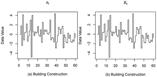
Figure 1. (a): The sample path of series $x_t$. (b): The sample plot of centering series $X_t$ for the real data.

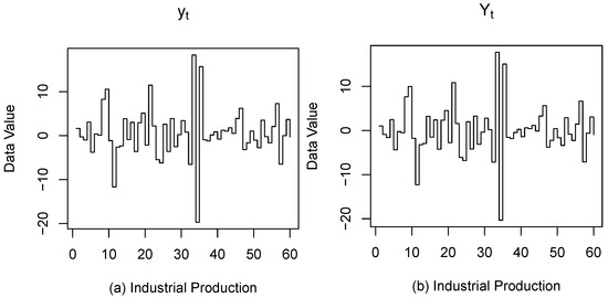
Figure 2. (a): The sample path of series $y_t$. (b): The sample plot of centering series $Y_t$ for the real data.

After transforming these two data sets, the resulting data with $X_t=x_t-E\left(x_t\right)$ and $Y_t=y_t-E\left(y_t\right)$ can be modeled using a BAR model. In addition, the plots of the autocorrelation function (ACF) and partial autocorrelation function (PACF) of sequences $\left\{X_t\right\}$ and $\left\{Y_t\right\}$ are given in Figure 3 and Figure 4, respectively. From Figure 4, it can be seen that these two sets of data come from a binary first-order autoregressive process. Therefore, it is reasonable to model the data with BAR(1), and it also shows that the proposed test statistic is valid for both sets of actual data. From Figure 1 and Figure 2 , it is unknown whether the parameters are constant or not; therefore, we consider the following test problem with the help of the proposed test statistic $T\left(\theta \right):$

$$H_0:\sum ={\sigma }_{{\alpha }_1}^2+{\sigma }_{{\alpha }_2}^2=0⟷H_1:\sum ={\sigma }_{{\alpha }_1}^2+{\sigma }_{{\alpha }_2}^2>0.$$

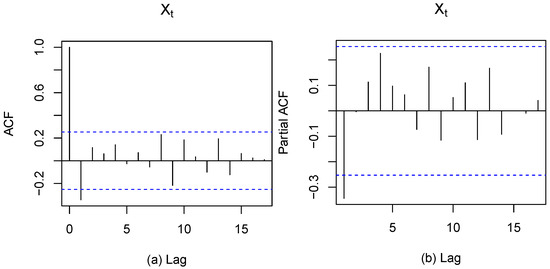
Figure 3. (a): The sample ACF plot of $X_t$. (b): The sample PACF plot of $X_t$.

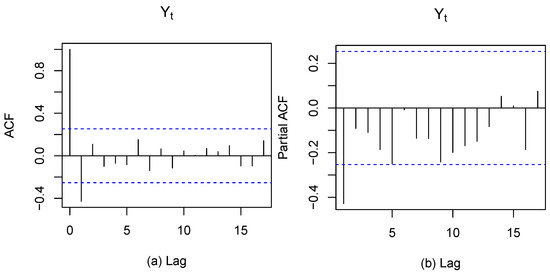
Figure 4. (a): The sample ACF plot of $Y_t$. (b): The sample PACF plot of $Y_t$.

The test statistic value in (5) is 33.21573 with a p-value of 0.00104, which is less than 0.05. This result indicates that we are rejecting the null hypothesis at the $5\%$ significance level. Therefore, the BRCAR(1) model is more appropriate than the BAR(1) model in this case.

4.2. Import and Export Data

The data represent the month-on-month growth rates of Japan’s export volume and import volume, respectively, from November 2012 to February 2020 (available at https://ceidata.cei.cn/new, accessed on 3 April 2024). The data of the month-on-month chain growth rate of exports are denoted as $x_1,x_2,\cdots ,x_{88}$, and the month-on-month chain growth rate of imports are denoted as $y_1,y_2,\cdots ,y_{88}$. We observe that $E\left(x_t\right)=-0.04034;$$E\left(y_t\right)=-0.23352;$$Var\left(x_t\right)=9.9499;$ $Var\left(y_t\right)=15.80747;$ ${\rho }_{x_t{y}_t}=0.222839.$ Figure 5 and Figure 6 shows a sample path diagram and sample centering series for the two data sets.

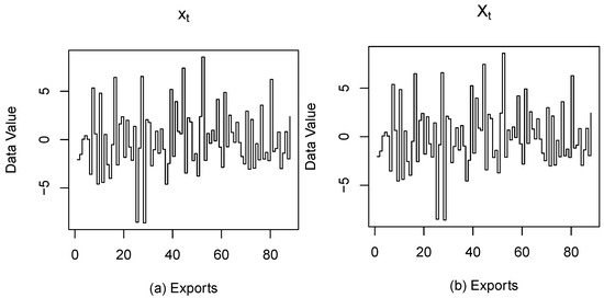
Figure 5. (a): The sample path of series $x_t$. (b): The sample plot of centering series $X_t$ for the real data.

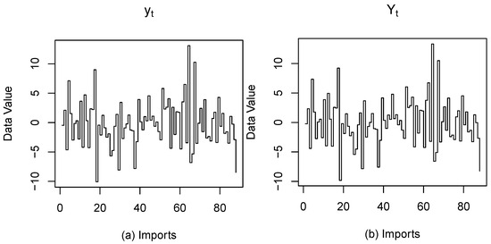
Figure 6. (a): The sample path of series $y_t$. (b): The sample plot of centering series $Y_t$ for the real data.

Similarly, the data with $X_t=x_t-E\left(x_t\right)$ and $Y_t=y_t-E\left(y_t\right)$ can be modeled using a BAR model. Furthermore, the plots of the $ACF$ and the $PACF$ of sequences $\left\{X_t\right\}$ and $\left\{Y_t\right\}$ are given in Figure 7 and Figure 8, respectively. From Figure 8, we can see that these two data sets come from a binary first-order autoregressive process. From the time series plot given in Figure 5 and Figure 6, the randomness of the parameter may be questioned; consequently, it is important to test the hypothesis of the randomness of the parameter. Similarly, we consider the following test problem with the help of the proposed test statistic $T\left(\theta \right):$

$$H_0:\sum ={\sigma }_{{\alpha }_1}^2+{\sigma }_{{\alpha }_2}^2=0⟷H_1:\sum ={\sigma }_{{\alpha }_1}^2+{\sigma }_{{\alpha }_2}^2>0.$$

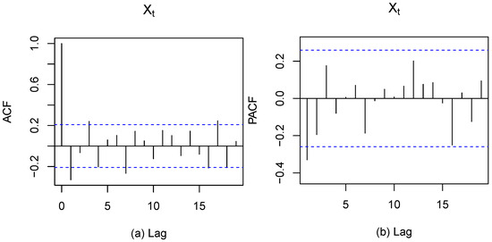
Figure 7. (a): The sample ACF plot of $X_t$. (b): The sample PACF plot of $X_t$.

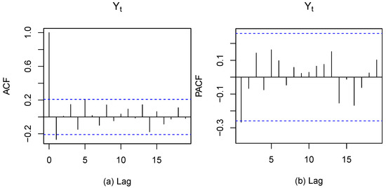
Figure 8. (a): The sample ACF plots of $Y_t$. (b): The sample PACF plot of $Y_t$.

The test statistic value in (5) is 6.905108 with a p-value of 0.03166, which is less than 0.05. Consequently, we are rejecting the null hypothesis at the $5\%$ significance level. Thus, modeling these data with the BRCAR(1) model is preferred over the BAR(1) model.

5. Conclusions

This paper proposes a locally most powerful-type test for testing the constancy of the random coefficient parameters in multivariate autoregressive models. We derive the test statistic and its limiting distribution under the null hypothesis. In practical applications, the coefficients of autoregressive models may not remain constant throughout the entire time period. Therefore, it is necessary to conduct such tests whenever there is a possibility of random variation in the coefficients. Through simulation studies and an analysis of real data, we demonstrate the effectiveness of our testing method and show that its performance surpasses that of competing methods. Finally, we anticipate that our LMP test can be extended and applied to other similar types of time series models.

References

- George, U. Vii. on a method of investigating periodicities disturbed series, with special reference to wolfer’s sunspot numbers. Philos. Trans. R. Soc. Lond. 1927, 226, 267–298. [Google Scholar] [CrossRef]
- George, E.B.; Gwilym, M.J.; Gregory, C.R.; Greta, M.L. Time Series Analysis: Forecasting and Control; John Wiley & Sons: Washington, DC, USA, 2015. [Google Scholar]
- Mohsen, M.; Nematollahi, A.R. Autoregressive models with mixture of scale mixtures of gaussian innovations. Iran. J. Sci. Technol. Trans. Sci. 2017, 41, 1099–1107. [Google Scholar] [CrossRef]
- Dmitry, P. Short-term traffic forecasting using multivariate autoregressive models. Procedia Eng. 2017, 178, 57–66. [Google Scholar] [CrossRef]
- Matthieu, G.; Adrià Tauste, C.; Xing, C.; Alexander, T.; Gustavo, D. Nonparametric test for connectivity detection in multivariate autoregressive networks and application to multiunit activity data. Netw. Neurosci. 2017, 1, 357–380. [Google Scholar] [CrossRef]
- Jiří, A. Autoregressive series with random parameters. Math. Oper. Und Stat. 1976, 7, 735–741. [Google Scholar] [CrossRef]
- Paul, D.F.; Richard, L.T. Random coefficient autoregressive processes: A markov chain analysis of stationarity and finiteness of moments. J. Time Ser. Anal. 1985, 6, 1–14. [Google Scholar] [CrossRef]
- Alexander, A.; Lajos, H.; Josef, S. Estimation in random coefficient autoregressive models. J. Time Ser. Anal. 2006, 27, 61–76. [Google Scholar] [CrossRef]
- Alexander, A.; Lajos, H. Quasi-likelihood estimation in stationary and nonstationary autoregressive models with random coefficients. Stat. Sin. 2011, 21, 973–999. [Google Scholar] [CrossRef]
- Holger, D.; Dominik, W. Detecting relevant changes in time series models. J. R. Stat. Soc. Ser. Stat. Methodol. 2016, 78, 371–394. [Google Scholar] [CrossRef]
- Lajos, H.; Lorenzo, T. Testing for randomness in a random coefficient autoregression model. J. Econom. 2019, 209, 338–352. [Google Scholar] [CrossRef]
- Li, B.; Feilong, L.; Kai, Y.; Dehui, W. Locally most powerful test for the random coefficient autoregressive model. Math. Probl. Eng. 2019, 1, 1099–1107. [Google Scholar] [CrossRef]
- Dazhe, W.; Sujit, K.G.; Sastry, G.P. Maximum likelihood estimation and unit root test for first order random coefficient autoregressive models. J. Stat. Theory Pract. 2010, 4, 261–278. [Google Scholar] [CrossRef]
- Jin, C.; Dehui, W.; Cong, L.; Jingwen, H. Estimation and testing of multivariate random coefficient autoregressive model based on empirical likelihood. Commun.-Stat.-Simul. Comput. 2023, 52, 291–308. [Google Scholar] [CrossRef]
- Zuzana, P.; Pavel, V. On a class of estimators in a multivariate rca (1) model. Kybernetika 2011, 47, 501–551. [Google Scholar] [CrossRef]
- Pavel, V. Rate of convergence for a class of rca estimators. Kybernetika 2006, 42, 699–709. [Google Scholar] [CrossRef]
- Des, F.N.; Barry, G.Q. Random COEFFICIENT Autoregressive Models: An Introduction; Springer Science & Business Media: New York, NY, USA, 1982. [Google Scholar]
- Awale, M.; Balakrishna, N.; Ramanathan, T.V. Testing the constancy of the thinning parameter in a random coefficient integer autoregressive model. Stat. Pap. 2019, 60, 1515–1539. [Google Scholar] [CrossRef]
- Chikkagoudar, M.S.; Biradar, B.S. Locally most powerful rank tests for comparison of two failure rates based on multiple type-ii censored data. Commun.-Stat.-Theory Methods 2012, 41, 4315–4331. [Google Scholar] [CrossRef]
- Rohatgi, V.K.; Md Ehsanes Sleh, A.K.; Ahluwalia, R.; Ji, P. Locally most powerful tests for the two sample problem when the combined sample is type ii censored. Commun.-Stat.-Theory Methods 1990, 19, 2337–2355. [Google Scholar] [CrossRef]
- Patrick, B. The lindeberg-levy theorem for martingales. Proc. Am. Math. Soc. 1961, 12, 788–792. [Google Scholar] [CrossRef]
- Peter, H.; Christopher, C.H. Martingale Limit Theory and Its Application; Academic Press: Washington, DC, USA, 2014. [Google Scholar]
- Zhang, H.; Wang, D.; Zhu, F. The empirical likelihood for first-order random coeffi cient integer-valued autoregressive processes. Commun. Stat. Theory Methods 2011, 40, 492–509. [Google Scholar] [CrossRef]
Disclaimer/Publisher’s Note: The statements, opinions and data contained in all publications are solely those of the individual author(s) and contributor(s) and not of MDPI and/or the editor(s). MDPI and/or the editor(s) disclaim responsibility for any injury to people or property resulting from any ideas, methods, instructions or products referred to in the content. |
© 2024 by the authors. Licensee MDPI, Basel, Switzerland. This article is an open access article distributed under the terms and conditions of the Creative Commons Attribution (CC BY) license (https://creativecommons.org/licenses/by/4.0/).