Riemann Problem for the Isentropic Euler Equations of Mixed Type in the Dark Energy Fluid

Abstract

We are concerned with the Riemann problem for the isentropic Euler equations of mixed type in the dark energy fluid. This system is non-strictly hyperbolic on the boundary curve of elliptic and hyperbolic regions. We obtain the unique admissible shock waves by utilizing the viscosity criterion. Assuming fixed left states are in the elliptic and hyperbolic regions, respectively, we construct the unique Riemann solution for the mixed-type models with the initial right state in some feasible regions. Finally, we present numerical simulations which are consistent with our theoretical results.

1. Introduction

In this paper, we consider the isentropic Euler equations of gas dynamics as follows:

$$\left\{\begin{array}{c}{\rho }_t+{\left(\rho u\right)}_x=0,\hfill \\ {\left(\rho u\right)}_t+{\left(\rho u^2+p\left(\rho \right)\right)}_x=0,\hfill \end{array}\right.(t,x)\in {\mathbb{R}}^{+}\times \mathbb{R},$$

(1)

with the equation of state (EoS)

$$p\left(\rho \right)=\rho ln\rho ,\rho >0,$$

(2)

where $\rho$, u, and p represent the density, the velocity, and the pressure, respectively [1]. System (1) with the EoS

$$p\left(\rho \right)=A\rho ln\left(B{\displaystyle \frac{\rho }{H^2}}\right)+C{\rho }^2+D{\displaystyle \frac{1}{\rho }}+E\rho$$

(3)

is called a dark energy fluid system, where A to E are constants, and H denotes the Hubble rate of our universe [2]. The use of a generalized dark energy EoS (3) makes possible the existence of de Sitter attractors, which has significant implications for understanding the nature of our universe. The dark energy fluid (3) is also used to describe the scenarios of dark matter–dark energy interaction [3]. In our work, we mainly study the Riemann solutions of dark energy (1) in terms of a logarithmic-corrected power-law fluid, that is, (2), which is a special form of (3) satisfying $A=B=H=1$ and $C=D=E=0$. It is interesting that the EoS of (2) may have a deep relation with equations of state found in condensed matter fluids [4].

It is well known that the system (1) is the isentropic Euler equations of gas dynamics. The pressure $p\left(\rho \right)$ varies for different models. The system (1) for the ideal polytropic gas satisfies $p=p_0{\rho }^{\gamma }$, where $p_0>0$ and $\gamma \ge 1$ is the adiabatic exponent. It was well studied in [1,5,6,7,8,9,10,11,12,13]. If the pressure $p=-{\displaystyle \frac{a}{{\rho }^{\mu }}}$, $a>0$, $\mu \in (0,1]$, it is the generalized Chaplygin gas model in [14], which is a proposal to explain the origin of dark energy as well as dark matter through a single fluid. For $\mu =1$, it is for the Chaplygin gas model, and $\delta$-shock waves may occur for the Riemann problem [15]. With $p=Aln\rho$, it has been introduced as a natural and robust candidate for a new unification of dark matter and dark energy [16]. It is also used to describe our universe filled with a single dark fluid [17]. For the above models, $p\left(\rho \right)$ is strictly increasing, which means that the system is globally hyperbolic. Noting that the isentropic Euler equations with the terms from (3), such as ${\rho }^2$, $-{\displaystyle \frac{1}{\rho }}$, and $\rho$, have been well studied, we are interested in the Riemann solutions for the isentropic Euler equations (1) with the EoS (2). To our knowledge, there are no related results. Since (2) is not monotonous any more, (1) and (2) are the isentropic Euler equations of mixed type.

The pathology of mixed-type systems concerns the ill-posedness [18] of the initial value problem. More precisely, there is no uniqueness of the Riemann problem if one considers the whole set of admissible solutions [19]. For example, the pressure of van der Waals fluid [20,21] is

$$p={\displaystyle \frac{RT}{v-b}}-{\displaystyle \frac{a}{v^2}},$$

(4)

where $v={\displaystyle \frac{1}{\rho }}$ denotes the specific volume. Considering the Riemann data

$${(\rho ,u)}_{t=0}=\left\{\begin{array}{c}({\rho }_l,u_l),x<0,\hfill \\ ({\rho }_r,u_r),x>0,\hfill \end{array}\right.$$

(5)

satisfying ${\rho }_l<\alpha <\beta <{\rho }_r$, where $\alpha$ and $\beta$ are constants such that $p^{\prime }\left(\rho \right)>0$ for $\rho \notin [\alpha ,\beta ]$ and $p^{\prime }\left(\rho \right)<0$ for $\rho \in (\alpha ,\beta )$, it was often used to study the phase transitions. In Lagrangian coordinates, (1) is transformed into

$$\left\{\begin{array}{c}{v}_t-u_x=0,\hfill \\ u_t+p{\left(v\right)}_x=0,\hfill \end{array}\right.$$

(6)

which is called a $p-$system. There exist multiple Riemann solutions for (4) and (6) with (5) because of the stationary shocks [22] or nonclassical shocks [23]. The nonclassical shocks violate the classic Lax entropy condition [24] and Liu entropy condition [25]. For more models which contain both hyperbolic and elliptic regions, the reader is referred to [26,27,28,29,30,31,32,33,34,35,36].

System (1) with (2) is hyperbolic for $\rho \ge 1/\mathrm{e}$ and elliptic for $0\le \rho <1/\mathrm{e}$. It is different from the van der Waals fluid model [19,23]. There is only one hyperbolic region for (1) with (2). However, in van der Waals fluid, there are two hyperbolic regions $(0,\alpha ]$ and $[\beta ,+\infty )$ where the Riemann solvers preserve the kinetic function [19]. In addition, system (1) with (2) is also different from the hyperbolic conservation laws [37]. The Lax entropy condition and the Liu entropy condition may not make sense in an elliptic region. Thus, if the initial left state (5) is in the elliptic region, we need a new entropy condition to guarantee the uniqueness.

In this paper, we provide the viscosity admissibility criterion to pick the admissible shock waves when the initial states (5) are in the elliptic region. According to the monotonicity of density $\rho$ in a travelling wave, we obtain an entropy condition which makes sense for the disconnected Hugoniot curve and self-interaction Hugoniot curve. If the initial states (5) are in the hyperbolic region, we obtain that it is equivalent to the classical Lax entropy condition. In addition, we obtain the unique Riemann solutions for the initial data in the feasible region. Finally, we present the numerical simulations for the solutions. The Gibbs phenomenon [38] appears at the boundary of the shock wave in the Euler equations of mixed type.

The paper is organized as follows. In Section 2, we introduce some basic quantities and properties for (1) and (2). In Section 3, we obtain the Hugoniot curves by the Rankine–Hugoniot conditions. Then, we propose an entropy condition by the viscosity criterion to obtain the admissible shock waves. In Section 4, the rarefaction waves are obtained through the Riemann invariants. In Section 5, the unique Riemann solutions for the initial states (5) in the solvable regions are constructed by the elementary waves. In Section 6, we present numerical tests to verify our theoretical results. In Section 7, we give a discussion about further work. In Section 8, we give a conclusion.

2. Preliminaries

In this section, we introduce the basic quantities and properties for (1) and (2). For the smooth solution, we know that (1) is equal to the following equations:

$$\left\{\begin{array}{c}{\rho }_t+u{\rho }_x+\rho u_x=0,\hfill \\ u_t+{\displaystyle \frac{ln\rho +1}{\rho }}{\rho }_x+u{u}_x=0.\hfill \end{array}\right.$$

(7)

The eigenvalues are

$${\lambda }_1\left(\rho ,u\right)=u-\sqrt{ln\rho +1},{\lambda }_2\left(\rho ,u\right)=u+\sqrt{ln\rho +1}.$$

(8)

If $\rho \ge {\displaystyle \frac{1}{\mathrm{e}}}$, the system is hyperbolic. In particular, if $\rho ={\displaystyle \frac{1}{\mathrm{e}}}$, the system is non-strictly hyperbolic, that is, ${\lambda }_1\left({\displaystyle \frac{1}{\mathrm{e}}},u\right)={\lambda }_2\left({\displaystyle \frac{1}{\mathrm{e}}},u\right)=u$. And if $0<\rho <{\displaystyle \frac{1}{\mathrm{e}}}$, the system is elliptic. Hereafter, we take $m=\rho u$. On the $(\rho ,m)$ plane, we divide the plane into four pieces as in Figure 1, where the elliptic region satisfies

$$\begin{array}{c}\hfill E=\{(\rho ,m)|0<\rho <{\displaystyle \frac{1}{\mathrm{e}}}\},\end{array}$$

and the hyperbolic region satisfies $H=H_1\bigcup H_2\bigcup H_3$ with

$$\begin{array}{c}\hfill H_1=\{(\rho ,m)|\rho \ge {\displaystyle \frac{1}{\mathrm{e}}},0<{\lambda }_1<{\lambda }_2\},\\ \hfill H_2=\{(\rho ,m)|\rho \ge {\displaystyle \frac{1}{\mathrm{e}}},{\lambda }_1<0<{\lambda }_2\},\\ \hfill H_3=\{(\rho ,m)|\rho \ge {\displaystyle \frac{1}{\mathrm{e}}},{\lambda }_1<{\lambda }_2<0\}.\end{array}$$

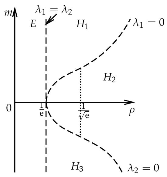
Figure 1. The elliptic region E and the hyperbolic regions $H_1$, $H_2$, and $H_3$.

The corresponding right vectors are

$${\overrightarrow{r}}_1={\left(-1,{\displaystyle \frac{\sqrt{ln\rho +1}}{\rho }}\right)}^T,{\overrightarrow{r}}_2={\left(1,{\displaystyle \frac{\sqrt{ln\rho +1}}{\rho }}\right)}^T.$$

(9)

According to

$$\nabla {\lambda }_1\left(\rho ,u\right)·{\overrightarrow{r}}_1=\nabla {\lambda }_2\left(\rho ,u\right)·{\overrightarrow{r}}_2={\displaystyle \frac{1}{2\rho \sqrt{ln\rho +1}}}+{\displaystyle \frac{\sqrt{ln\rho +1}}{\rho }}>0,$$

(10)

we know that this system (1) with (2) is genuinely nonlinear when the states are in the hyperbolic region. Moreover, according to the definition of the Riemann invariants [37] which satisfy $\nabla {\omega }_i·{\overrightarrow{r}}_i=0$, $i=1,2$, we obtain the two Riemann invariants as follows:

$$\left\{\begin{array}{c}{\omega }_1={\displaystyle \frac{m}{\rho }}+{\displaystyle \frac{2}{3}}{\left(ln\rho +1\right)}^{{\displaystyle \frac{3}{2}}},\hfill \\ {\omega }_2={\displaystyle \frac{m}{\rho }}-{\displaystyle \frac{2}{3}}{\left(ln\rho +1\right)}^{{\displaystyle \frac{3}{2}}}.\hfill \end{array}\right.$$

(11)

3. Shock Waves

In this section, we devote ourselves to the admissible shock waves. We first obtain the possible discontinuity curves in Section 3.1. Then, by the viscosity criterion, we propose the entropy condition (32) in Section 3.2. Finally, for the fixed left state (5) in different regions, we provide the shock wave curves and their properties on the $(\rho ,m)$ phase plane in Section 3.3.

3.1. Discontinuity Curves

Let $x\left(t\right)$ be the discontinuity curve. By the Rankine–Hugoniot (R-H) conditions [37],

$$\left\{\begin{array}{c}\left[\rho \right]{\displaystyle \frac{\mathrm{d}x}{\mathrm{d}t}}=\left[m\right],\hfill \\ \left[m\right]{\displaystyle \frac{\mathrm{d}x}{\mathrm{d}t}}=[{\displaystyle \frac{m^2}{\rho }}+p\left(\rho \right)],\hfill \end{array}\right.$$

(12)

where $\left[a\right]=a-a_l$, we have that if $\left[\rho \right]=0$, then it holds that $\left[m\right]=0$. The trivial solution is constant. If $\left[\rho \right]\ne 0$, we have that

$${\left[m\right]}^2=\left[\rho \right]\left[{\displaystyle \frac{m^2}{\rho }}+p\left(\rho \right)\right].$$

(13)

It means that

$$\rho {\rho }_l{\left({\displaystyle \frac{m}{\rho }}-{\displaystyle \frac{m_l}{{\rho }_l}}\right)}^2=\left(\rho -{\rho }_l\right)\left(p\left(\rho \right)-p\left({\rho }_l\right)\right),$$

(14)

which is called the Hugoniot curve. Thus, the right side of (14) should hold that

$$\left(\rho -{\rho }_l\right)\left(p\left(\rho \right)-p\left({\rho }_l\right)\right)\ge 0.$$

(15)

We now discuss the sufficient condition of (15) with the fixed ${\rho }_l$. According to (2), we know that $p^{\prime }\left(\rho \right)=ln\rho +1$ and $p^{″}\left(\rho \right)={\displaystyle \frac{1}{\rho }}$. Then, we depict the pressure p in Figure 2.

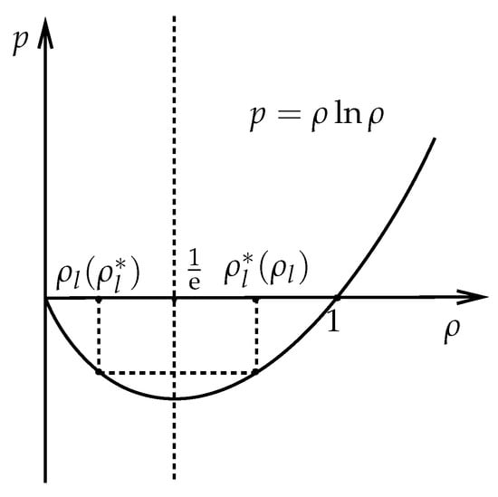
Figure 2. The picture of $p=\rho ln\rho$, where ${\rho }_l^{\ast }ln{\rho }_l^{\ast }={\rho }_{l}ln{\rho }_l$ when $0<{\rho }_l<1$.

If $0<{\rho }_l<1$, there is always a ${\rho }_l^{\ast }$ satisfying $p\left({\rho }_l^{\ast }\right)=p\left({\rho }_l\right)$, that is, ${\rho }_l^{\ast }ln{\rho }_l^{\ast }={\rho }_{l}ln{\rho }_l$. From Figure 2, all the points satisfying $\rho >{\rho }_l^{\ast }$ make (15) hold. If the fixed ${\rho }_l\ge 1$, those points satisfying $\rho >{\rho }_l$ make (15) hold. Then, there are two discontinuity curves satisfying

$${\displaystyle \frac{m}{\rho }}-{\displaystyle \frac{m_l}{{\rho }_l}}=\pm \sqrt{{\displaystyle \frac{\left(\rho -{\rho }_l\right)\left(\rho ln\rho -{\rho }_{l}ln{\rho }_l\right)}{\rho {\rho }_l}}},$$

(16)

or

$${\displaystyle \frac{m-m_l}{\rho -{\rho }_l}}={\displaystyle \frac{m_l}{{\rho }_l}}\pm \sqrt{{\displaystyle \frac{\rho \left(\rho ln\rho -{\rho }_{l}ln{\rho }_l\right)}{{\rho }_l\left(\rho -{\rho }_l\right)}}}.$$

(17)

We depict the Hugoniot curves (16) or (17) as in Figure 3 for three cases with ${\rho }_l$ in different regions: (a) $0<{\rho }_l<{\displaystyle \frac{1}{\mathrm{e}}}$, (b) ${\displaystyle \frac{1}{\mathrm{e}}}\le {\rho }_l<1$, (c) ${\rho }_l\ge 1$, respectively.

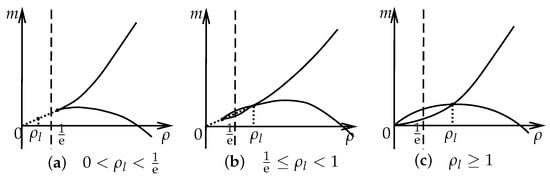
Figure 3. The Hugoniot curves with ${\rho }_l$ in different regions. For case (a): $0<{\rho }_l<{\displaystyle \frac{1}{\mathrm{e}}}$ and (b): ${\displaystyle \frac{1}{\mathrm{e}}}\le {\rho }_l<1$; it holds that $\rho >{\rho }_l^{\ast }$. For case (c): ${\rho }_l\ge 1$; it holds that $\rho >0$.

From Figure 3, if the initial left state is in the hyperbolic region, the Hugoniot curve of the mixed system (1) with (2) is not a simple curve. The initial left state is the self-intersection point of the Hugoniot curve. If the initial left state is in the elliptic region, the Hugoniot curve is not continuous. The initial left state is an isolated point.

3.2. Admissible Criterion

In this subsection, we consider the admissibility of the discontinuity curves by the viscosity criterion [39]. The viscosity system of (1) takes the form

$$\left\{\begin{array}{c}{\rho }_t+m_x=\epsilon {\rho }_{xx},\hfill \\ m_t+{\left({\displaystyle \frac{m^2}{\rho }}+\rho ln\rho \right)}_x=0,\hfill \end{array}\right.$$

(18)

where $\epsilon$ is the assumed viscosity constant. Assume that $(s;{\rho }_l,m_l;{\rho }_r,m_r)$ satisfies the R-H conditions (12), where s denotes the shock speed. This discontinuity curve is said to be admissible according to the viscosity criterion if the wave is a limit as $\epsilon \to 0^{+}$ of the traveling wave solution $(P\left({\displaystyle \frac{x-st}{\epsilon }}\right),M\left({\displaystyle \frac{x-st}{\epsilon }}\right))$ of the system (18) with the boundary condition

$$(P(-\infty ),M(-\infty );P(+\infty ),M(+\infty ))=({\rho }_l,m_l;{\rho }_r,m_r),$$

(19)

where $({\rho }_l,m_l;{\rho }_r,m_r)$ satisfies (16), ${\rho }_r\ne {\rho }_l$ and ${\rho }_r\ge {\rho }_l^{\ast }$. For simplicity of notation, we use $\zeta$ instead of ${\displaystyle \frac{x-st}{\epsilon }}$. Then, the viscosity system (18) becomes

$$\left\{\begin{array}{c}{P}^{\prime }(-s)+M^{\prime }=P^{\prime \prime },\hfill \\ M^{\prime }(-s)+{\left({\displaystyle \frac{M^2}{P}}+PlnP\right)}^{\prime }=0,\hfill \end{array}\right.$$

(20)

where ${ }^{\prime }={\displaystyle \frac{\mathrm{d}}{\mathrm{d}\zeta }}$. We have that

$$P^{\prime }(-s^2)+{\left({\displaystyle \frac{M^2}{P}}+PlnP\right)}^{\prime }=s{P}^{″}.$$

(21)

The integration of the first equation of (20) and (21) from $-\infty$ to $\zeta$ coupled with (19) yields

$$\left\{\begin{array}{c}(P\left(\zeta \right)-{\rho }_l)(-s)+M\left(\zeta \right)-m_l=P^{\prime }\left(\zeta \right),\hfill \\ (P\left(\zeta \right)-{\rho }_l)(-s^2)+\left({\displaystyle \frac{M^2}{P}}+PlnP\right)\left(\zeta \right)-c=s{P}^{\prime }\left(\zeta \right),\hfill \end{array}\right.$$

(22)

where $c={\displaystyle \frac{m_l^2}{{\rho }_l}}+{\rho }_{l}ln{\rho }_l$. Then, we have the following result.

Lemma 1.

The traveling wave solution $P\left(\zeta \right)$ of (20), which connects the left state ${\rho }_l$ and right state ${\rho }_r$, is strictly monotonous.

Proof of Lemma 1. 

We now prove that there is no point such that $P^{\prime }\left(\zeta \right)=0$. Using proof by contradiction, we assume that there is a ${\zeta }_0$ satisfying $P\left({\zeta }_0\right)=P_0$ and $P^{\prime }\left({\zeta }_0\right)=0$, where $P_0\ne {\rho }_l,{\rho }_r$. Then, at ${\zeta }_0$, we have that

$${(s-{\displaystyle \frac{m_l}{{\rho }_l}})}^2={\displaystyle \frac{P_0(P_{0}ln{P}_0-{\rho }_{l}ln{\rho }_l)}{{\rho }_l(P_0-{\rho }_l)}}$$

(23)

by (22). Because of $P^{\prime }(-\infty )=P^{\prime }(+\infty )=0$, it holds that

$$s={\displaystyle \frac{m_r-m_l}{{\rho }_r-{\rho }_l}}$$

(24)

by the first equation of (22). Connected with (17), we have that

$${(s-{\displaystyle \frac{m_l}{{\rho }_l}})}^2={\displaystyle \frac{{\rho }_r({\rho }_{r}ln{\rho }_r-{\rho }_{l}ln{\rho }_l)}{{\rho }_l({\rho }_r-{\rho }_l)}}.$$

(25)

Thus, by (23) and (25), it should hold that

$${\displaystyle \frac{{\rho }_r({\rho }_{r}ln{\rho }_r-{\rho }_{l}ln{\rho }_l)}{{\rho }_r-{\rho }_l}}={\displaystyle \frac{P_0(P_{0}ln{P}_0-{\rho }_{l}ln{\rho }_l)}{{\rho }_l(P_0-{\rho }_l)}}.$$

(26)

Let

$$G\left(\rho \right)={\displaystyle \frac{\rho \left(\rho ln\rho -{\rho }_{l}ln{\rho }_l\right)}{\rho -{\rho }_l}};$$

(27)

then, we know that

$$G^{\prime }\left(\rho \right)={\displaystyle \frac{\rho (ln\rho +1)-{\rho }_l\frac{\rho ln\rho -{\rho }_{l}ln{\rho }_l}{\rho -{\rho }_l}}{\rho -{\rho }_l}}.$$

(28)

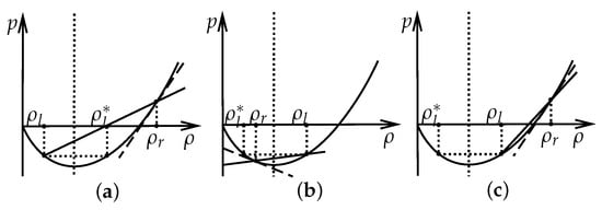
Because in (28), $ln\rho +1$ represents the slope of the tangent line to the curve p at the point $\rho$, and ${\displaystyle \frac{\rho ln\rho -{\rho }_{l}ln{\rho }_l}{\rho -{\rho }_l}}$ represents the slope of the secant line to the curve p passing through points $\rho$ and ${\rho }_l$, we next analyze the monotonicity of $G\left(\rho \right)$ by using the property of p. Now, we discuss three cases for the initial data.

Case 1. If $0<{\rho }_l<{\displaystyle \frac{1}{\mathrm{e}}}$, we know that ${\rho }_r\ge {\rho }_l^{\ast }>{\rho }_l$ and

$${\displaystyle \frac{{\rho }_{r}ln{\rho }_r-{\rho }_{l}ln{\rho }_l}{{\rho }_r-{\rho }_l}}\ge 0,$$

(29)

which means $P_0\ge {\rho }_l^{\ast }>{\rho }_l$ by (26). See Figure 4a. In Figure 4, the solid lines denote the secant lines which connect the left state ${\rho }_l$ and the right state ${\rho }_r$. The dashed lines denote the tangent line at the right state ${\rho }_r$.

Figure 4. The three cases for the initial data in different regions. (a) $0<{\rho }_l<{\displaystyle \frac{1}{\mathrm{e}}}, {\rho }_r>{\rho }_l^{\ast }$. (b) ${\rho }_l>{\displaystyle \frac{1}{\mathrm{e}}}, {\rho }_r<{\rho }_l$. (c) ${\rho }_l>{\displaystyle \frac{1}{\mathrm{e}}}, {\rho }_r>{\rho }_l$.

For all $\rho >{\rho }_l^{\ast }$, we have

$$ln\rho +1>{\displaystyle \frac{\rho ln\rho -{\rho }_{l}ln{\rho }_l}{\rho -{\rho }_l}},$$

(30)

where the left side is the slope of the tangent line at $\rho$, and the right side is the slope of the secant line from ${\rho }_l$ to $\rho$. Then, it holds that $G^{\prime }\left(\rho \right)>0$. Thus, (26) holds if and only if $P_0={\rho }_r$, which contradicts that $P_0$ is different from ${\rho }_r$.

Case 2. If ${\rho }_l\ge {\displaystyle \frac{1}{\mathrm{e}}}$, we know that ${\rho }_r\ge {\rho }_l^{\ast }$ and (29) holds, which means $P_0\ge {\rho }_l^{\ast }$ by (26). In this case, ${\rho }_l^{\ast }\le P_0<{\rho }_l$, then for any ${\rho }_l^{\ast }\le \rho <{\rho }_l$, it holds that

$$ln\rho +1<{\displaystyle \frac{\rho ln\rho -{\rho }_{l}ln{\rho }_l}{\rho -{\rho }_l}},$$

(31)

which means that $G^{\prime }\left(\rho \right)>0$. See Figure 4b.

Case 3. If ${\rho }_l\ge {\displaystyle \frac{1}{\mathrm{e}}}$ and ${\rho }_r>{\rho }_l$, which means $P_0>{\rho }_l$, then (30) holds, which also means that $G^{\prime }\left(\rho \right)>0$. See Figure 4c.

In conclusion, (26) holds if and only if $P_0={\rho }_r$, which contradicts that $P_0$ is different from ${\rho }_r$. We know that $P\left(\zeta \right)$ is strictly monotonous from $-\infty$ to $+\infty$. □

According to Lemma 1, if $P>{\rho }_l$, then it holds that $P^{\prime }\left(\zeta \right)>0$. If $P<{\rho }_l$, it holds that $P^{\prime }\left(\zeta \right)<0$. Thus, we have that ${\displaystyle \frac{P^{\prime }\left(\zeta \right)}{P-{\rho }_l}}>0$. For any P between ${\rho }_l$ and ${\rho }_r$, it holds that ${\displaystyle \frac{M-m_l}{P-{\rho }_l}}-{\displaystyle \frac{P^{\prime }\left(\zeta \right)}{P-{\rho }_l}}<{\displaystyle \frac{M-m_l}{P-{\rho }_l}}$. From the first equality of (22), we have that

$$s={\displaystyle \frac{m_r-m_l}{{\rho }_r-{\rho }_l}}<{\displaystyle \frac{m-m_l}{\rho -{\rho }_l}},\mathrm{as}\epsilon \to 0^{+}$$

(32)

for any $\rho$ between ${\rho }_l$ and ${\rho }_r$. As the viscosity admissibility criterion for a discontinuity, (32) is called the entropy condition.

3.3. Admissible Shock Waves

In this subsection, we pick up the unique admissible shock waves by the entropy condition (32) from the Hugoniot curves (16) and analyze the properties of them. Assume that the left state is $({\rho }_l,m_l)$ and the right state is $(\rho ,m)$. To solve the Riemann problem of (1) by a single shock wave, we categorize the initial data into four distinct cases, as follows: I, $\rho >{\rho }_l\ge {\displaystyle \frac{1}{\mathrm{e}}}$; II, $\rho >{\displaystyle \frac{1}{\mathrm{e}}}>{\rho }_l$; III, ${\rho }_l>\rho \ge {\displaystyle \frac{1}{\mathrm{e}}}$; IV, ${\rho }_l>{\displaystyle \frac{1}{\mathrm{e}}}>\rho$. Next, we analyze the shock waves case by case.

Case I. $\rho >{\rho }_l\ge {\displaystyle \frac{1}{\mathrm{e}}}$. It means that the initial data are in the hyperbolic region. To obtain the admissible shock wave, we pick it from the discontinuity curves (17) satisfying (32).

If the shock wave satisfies

$${\displaystyle \frac{m-m_l}{\rho -{\rho }_l}}={\displaystyle \frac{m_l}{{\rho }_l}}-\sqrt{{\displaystyle \frac{\rho \left(\rho ln\rho -{\rho }_{l}ln{\rho }_l\right)}{{\rho }_l\left(\rho -{\rho }_l\right)}}},$$

(33)

we have that

$$\begin{array}{c}\hfill \left\{\begin{array}{cc}{\displaystyle \frac{m_r-m_l}{{\rho }_r-{\rho }_l}}\hfill & ={\displaystyle \frac{m_l}{{\rho }_l}}-\sqrt{{\displaystyle \frac{{\rho }_r\left({\rho }_{r}ln{\rho }_r-{\rho }_{l}ln{\rho }_l\right)}{{\rho }_l\left({\rho }_r-{\rho }_l\right)}}},\hfill \\ {\displaystyle \frac{m-m_l}{\rho -{\rho }_l}}\hfill & ={\displaystyle \frac{m_l}{{\rho }_l}}-\sqrt{{\displaystyle \frac{\rho \left(\rho ln\rho -{\rho }_{l}ln{\rho }_l\right)}{{\rho }_l\left(\rho -{\rho }_l\right)}}},\hfill \end{array}\right.\end{array}$$

(34)

where the state $(\rho ,m)$ satisfies ${\rho }_l<\rho <{\rho }_r$. It holds that $G^{\prime }\left(\rho \right)>0$ where $G\left(\rho \right)$ satisfies (27).

Thus, it holds that

$${\displaystyle \frac{{\rho }_r\left({\rho }_{r}ln{\rho }_r-{\rho }_{l}ln{\rho }_l\right)}{{\rho }_r-{\rho }_l}}>{\displaystyle \frac{\rho \left(\rho ln\rho -{\rho }_{l}ln{\rho }_l\right)}{\rho -{\rho }_l}},$$

(35)

which means the shock wave satisfies the entropy condition (32). In addition, according to $\rho >{\rho }_l>{\displaystyle \frac{1}{\mathrm{e}}}$ and

$$ln{\rho }_l+1<{\displaystyle \frac{\rho ln\rho -{\rho }_{l}ln{\rho }_l}{\rho -{\rho }_l}}<ln\rho +1,$$

we know that the speed of the shock wave satisfies

$$s={\displaystyle \frac{m-m_l}{\rho -{\rho }_l}}=u_l-\sqrt{{\displaystyle \frac{\rho \left(\rho ln\rho -{\rho }_{l}ln{\rho }_l\right)}{{\rho }_l(\rho -{\rho }_l)}}}<u_l-\sqrt{ln{\rho }_l+1}={\lambda }_1({\rho }_l,u_l).$$

(36)

And it holds that

$$s={\displaystyle \frac{m-m_l}{\rho -{\rho }_l}}=u-\sqrt{{\displaystyle \frac{{\rho }_l\left(\rho ln\rho -{\rho }_{l}ln{\rho }_l\right)}{\rho (\rho -{\rho }_l)}}}>u-\sqrt{ln\rho +1}={\lambda }_1(\rho ,u).$$

(37)

Conditions (36) and (37) are the Lax entropy conditions for 1-shock waves.

If the shock wave satisfies

$${\displaystyle \frac{m-m_l}{\rho -{\rho }_l}}={\displaystyle \frac{m_l}{{\rho }_l}}+\sqrt{{\displaystyle \frac{\rho \left(\rho ln\rho -{\rho }_{l}ln{\rho }_l\right)}{{\rho }_l\left(\rho -{\rho }_l\right)}}},$$

(38)

we have that

$$\begin{array}{c}\hfill \left\{\begin{array}{cc}{\displaystyle \frac{m_r-m_l}{{\rho }_r-{\rho }_l}}\hfill & ={\displaystyle \frac{m_l}{{\rho }_l}}+\sqrt{{\displaystyle \frac{{\rho }_r\left({\rho }_{r}ln{\rho }_r-{\rho }_{l}ln{\rho }_l\right)}{{\rho }_l\left({\rho }_r-{\rho }_l\right)}}},\hfill \\ {\displaystyle \frac{m-m_l}{\rho -{\rho }_l}}\hfill & ={\displaystyle \frac{m_l}{{\rho }_l}}+\sqrt{{\displaystyle \frac{\rho \left(\rho ln\rho -{\rho }_{l}ln{\rho }_l\right)}{{\rho }_l\left(\rho -{\rho }_l\right)}}},\hfill \end{array}\right.\end{array}$$

(39)

where the state $(\rho ,m)$ satisfies ${\rho }_l<\rho <{\rho }_r$. Taking it into (32), it holds that

$${\displaystyle \frac{{\rho }_r\left({\rho }_{r}ln{\rho }_r-{\rho }_{l}ln{\rho }_l\right)}{{\rho }_r-{\rho }_l}}<{\displaystyle \frac{\rho \left(\rho ln\rho -{\rho }_{l}ln{\rho }_l\right)}{\rho -{\rho }_l}}.$$

(40)

It contradicts with (35) for ${\rho }_r>\rho >{\rho }_l>{\displaystyle \frac{1}{\mathrm{e}}}$. Thus, (38) is not an admissible shock wave.

Based on the above analysis, we obtain the 1-shock wave denoted by $S_1$, which satisfies

$$S_1({\rho }_l,m_l):\left\{\begin{array}{c}\begin{array}{c}{\displaystyle \frac{m-m_l}{\rho -{\rho }_l}}={\displaystyle \frac{m_l}{{\rho }_l}}-\sqrt{{\displaystyle \frac{\rho \left(\rho ln\rho -{\rho }_{l}ln{\rho }_l\right)}{{\rho }_l\left(\rho -{\rho }_l\right)}}},\rho >{\rho }_l\ge {\displaystyle \frac{1}{\mathrm{e}}},\hfill \\ {\lambda }_1(\rho ,u)<s<{\lambda }_1({\rho }_l,u_l).\hfill \end{array}\hfill \end{array}\right.$$

(41)

In addition, along the shock wave $S_1$, we have that

$${\displaystyle \frac{\mathrm{d}}{\mathrm{d}\rho }}\left({\displaystyle \frac{m-m_l}{\rho -{\rho }_l}}\right)=-{\displaystyle \frac{G^{\prime }\left(\rho \right)}{2\sqrt{{\rho }_{l}G\left(\rho \right)}}}<0,$$

(42)

where $G\left(\rho \right)$ is defined by (27). Now, we depict the 1-shock wave $S_1({\rho }_l,m_l)$ for the left state $({\rho }_l,m_l)$ in the hyperbolic region $H_1$ with a solid curve, as shown in Figure 5. Hereafter, we mark Ⓛ as the left state $({\rho }_l,m_l)$ shown in Figure 5. The dotted curves denote the shock waves $S_1({\rho }_l,m_l)$ from the left state $({\rho }_l,m_l)$, which is in hyperbolic region $H_2$ or $H_3$.

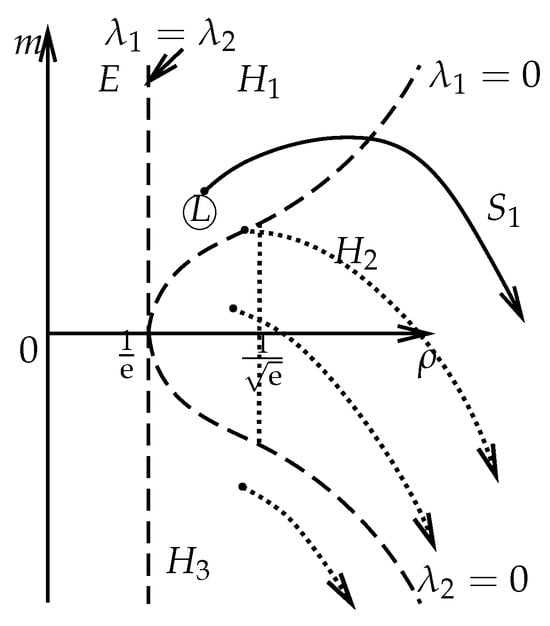
Figure 5. The first family shock wave $S_1({\rho }_l,m_l)$ if the left state $({\rho }_l,m_l)$ is in the hyperbolic region.

Remark 1.

For this case, if the left state is in the region of $H_1$ (see Figure 5), there is a stationary shock wave such that ${\displaystyle \frac{\mathrm{d}x}{\mathrm{d}t}}=0$, that is, $m=m_l$ and ${\displaystyle \frac{m^2}{\rho }}+\rho ln\rho ={\displaystyle \frac{m_l^2}{{\rho }_l}}+{\rho }_{l}ln{\rho }_l$.

Case II. $\rho >{\displaystyle \frac{1}{\mathrm{e}}}>{\rho }_l$. It means that the left state $({\rho }_l,u_l)$ is in the elliptical region and the right state $(\rho ,u)$ is in the hyperbolic region. There exists a unique ${\rho }_l^{\ast }>{\displaystyle \frac{1}{\mathrm{e}}}$ such that ${\rho }_l^{\ast }ln{\rho }_l^{\ast }={\rho }_{l}ln{\rho }_l$. If the discontinuity curve exists, it must hold that $\rho \ge {\rho }_l^{\ast }>{\displaystyle \frac{1}{\mathrm{e}}}>{\rho }_l$. For this case, the shock wave which should satisfy (17) is no longer a continuity curve. And there is a jump from the left state to the right state. Similar to Case I, according to the entropy condition (32), we obtain the 1-shock wave denoted by $S_1^E$ (see Figure 6) satisfying

$$S_1^E({\rho }_l,m_l):\left\{\begin{array}{c}\begin{array}{c}{\displaystyle \frac{m-m_l}{\rho -{\rho }_l}}={\displaystyle \frac{m_l}{{\rho }_l}}-\sqrt{{\displaystyle \frac{\rho \left(\rho ln\rho -{\rho }_{l}ln{\rho }_l\right)}{{\rho }_l\left(\rho -{\rho }_l\right)}}},\rho \ge {\rho }_l^{\ast }>{\displaystyle \frac{1}{\mathrm{e}}}>{\rho }_l,\hfill \\ {\lambda }_1(\rho ,u)<s\le u_l.\hfill \end{array}\hfill \end{array}\right.$$

(43)

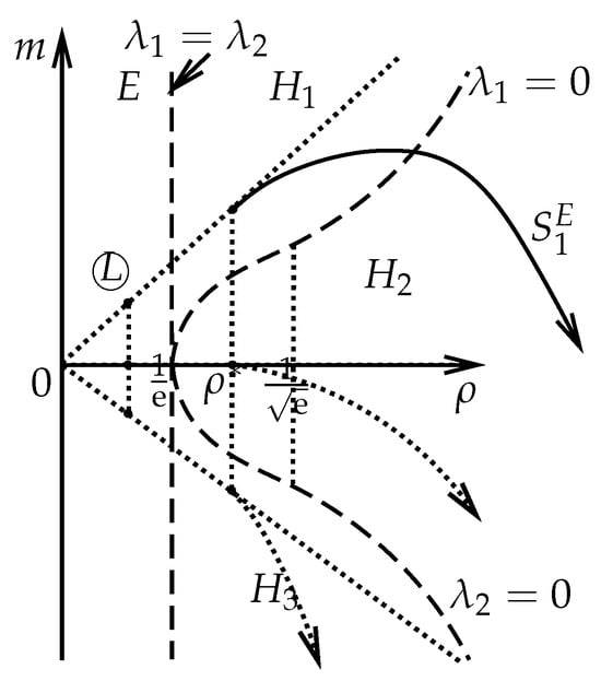
Figure 6. The first family shock wave $S_1^E$ if the left state $({\rho }_l,m_l)$ is in the elliptic region.

In Figure 6, the dotted curves denote the $S_1^E$ from $({\rho }_l^{\ast },m_l^{\ast })$ where the left state with the same ${\rho }_l$ and the different $m_l$ is in the elliptic region. Along this shock wave $S_1^E$, we have that

$${\displaystyle \frac{\mathrm{d}}{\mathrm{d}\rho }}\left({\displaystyle \frac{m-m_l}{\rho -{\rho }_l}}\right)=-{\displaystyle \frac{G^{\prime }\left(\rho \right)}{2\sqrt{{\rho }_{l}G\left(\rho \right)}}}<0.$$

(44)

Case III. ${\rho }_l>\rho \ge {\displaystyle \frac{1}{\mathrm{e}}}$. It means that both left and right states are in the hyperbolic region. Then, by the entropy condition (32), we obtain the 2-shock wave denoted by $S_2$ (see Figure 7), which satisfies

$$S_2({\rho }_l,m_l):\left\{\begin{array}{c}\begin{array}{c}{\displaystyle \frac{m-m_l}{\rho -{\rho }_l}}={\displaystyle \frac{m_l}{{\rho }_l}}+\sqrt{{\displaystyle \frac{\rho \left(\rho ln\rho -{\rho }_{l}ln{\rho }_l\right)}{{\rho }_l\left(\rho -{\rho }_l\right)}}},{\rho }_l>\rho \ge {\displaystyle \frac{1}{\mathrm{e}}},\hfill \\ {\lambda }_2(\rho ,u)<s<{\lambda }_2({\rho }_l,u_l).\hfill \end{array}\hfill \end{array}\right.$$

(45)

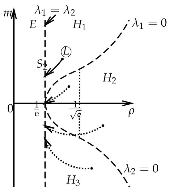
Figure 7. The second family shock wave $S_2$ if both the left state $({\rho }_l,m_l)$ and the right state are in the hyperbolic region.

The dotted curves denote the $S_2$ from the left state $({\rho }_l,m_l)$ in a different hyperbolic region. Along this shock wave $S_2$, we have that

$${\displaystyle \frac{\mathrm{d}}{\mathrm{d}\rho }}\left({\displaystyle \frac{m-m_l}{\rho -{\rho }_l}}\right)={\displaystyle \frac{G^{\prime }\left(\rho \right)}{2\sqrt{{\rho }_{l}G\left(\rho \right)}}}>0.$$

(46)

Case IV. ${\rho }_l>{\displaystyle \frac{1}{\mathrm{e}}}>\rho$. It means that the left state $({\rho }_l,u_l)$ is in the hyperbolic region and the right state $(\rho ,u)$ is in the elliptical region. There are two subcases.

Subcase IV.1. If ${\displaystyle \frac{1}{\mathrm{e}}}<{\rho }_l\le 1$, there exists a unique ${\rho }_l^{\ast }<{\displaystyle \frac{1}{\mathrm{e}}}$ such that ${\rho }_l^{\ast }ln{\rho }_l^{\ast }={\rho }_{l}ln{\rho }_l$. If the discontinuity curve exists, it must hold that ${\rho }_l>{\displaystyle \frac{1}{\mathrm{e}}}>\rho >{\rho }_l^{\ast }$. Then, according to the entropy condition (32), we obtain the 2-shock wave denoted by $S_2^E$ (see Figure 8) satisfying

$$S_2^E({\rho }_l,m_l):\left\{\begin{array}{c}\begin{array}{c}{\displaystyle \frac{m-m_l}{\rho -{\rho }_l}}={\displaystyle \frac{m_l}{{\rho }_l}}+\sqrt{{\displaystyle \frac{\rho \left(\rho ln\rho -{\rho }_{l}ln{\rho }_l\right)}{{\rho }_l\left(\rho -{\rho }_l\right)}}},{\rho }_l>{\displaystyle \frac{1}{\mathrm{e}}}>\rho >{\rho }_l^{\ast },\hfill \\ u\le s<{\lambda }_2({\rho }_l,u_l).\hfill \end{array}\hfill \end{array}\right.$$

(47)

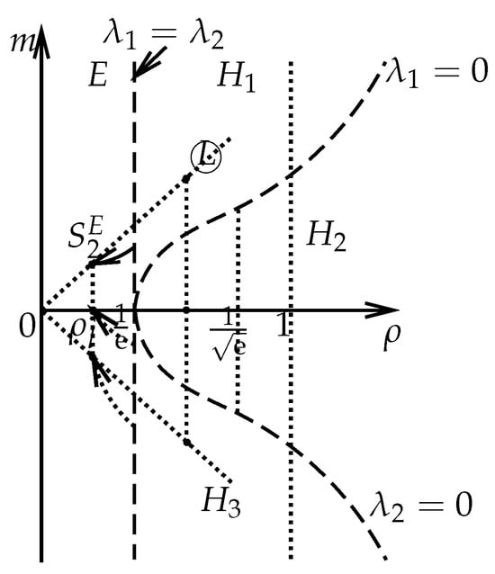
Figure 8. The second family shock wave $S_2^E$ for the left state $({\rho }_l,m_l)$ in the hyperbolic region and the right state in the elliptic region.

In Figure 8, the dotted curves denote the $S_2^E$ from the boundary of the elliptic region to the $({\rho }_l^{\ast },m_l^{\ast })$, where the left state $({\rho }_l,m_l)$ is in a different hyperbolic region with the same ${\rho }_l$ and different $m_l$. Along this shock wave $S_2^E$, we have that

$${\displaystyle \frac{\mathrm{d}}{\mathrm{d}\rho }}\left({\displaystyle \frac{m-m_l}{\rho -{\rho }_l}}\right)={\displaystyle \frac{G^{\prime }\left(\rho \right)}{2\sqrt{{\rho }_{l}G\left(\rho \right)}}}>0.$$

(48)

Subcase IV.2. If ${\rho }_l>1$, the 2-shock wave denoted by $S_2^{\overline{E}}$ (see Figure 9) satisfies

$$S_2^{\overline{E}}({\rho }_l,m_l):\left\{\begin{array}{c}\begin{array}{c}{\displaystyle \frac{m-m_l}{\rho -{\rho }_l}}={\displaystyle \frac{m_l}{{\rho }_l}}+\sqrt{{\displaystyle \frac{\rho \left(\rho ln\rho -{\rho }_{l}ln{\rho }_l\right)}{{\rho }_l\left(\rho -{\rho }_l\right)}}},{\rho }_l>1>{\displaystyle \frac{1}{\mathrm{e}}}>\rho >0,\hfill \\ u<s<{\lambda }_2({\rho }_l,u_l).\hfill \end{array}\hfill \end{array}\right.$$

(49)

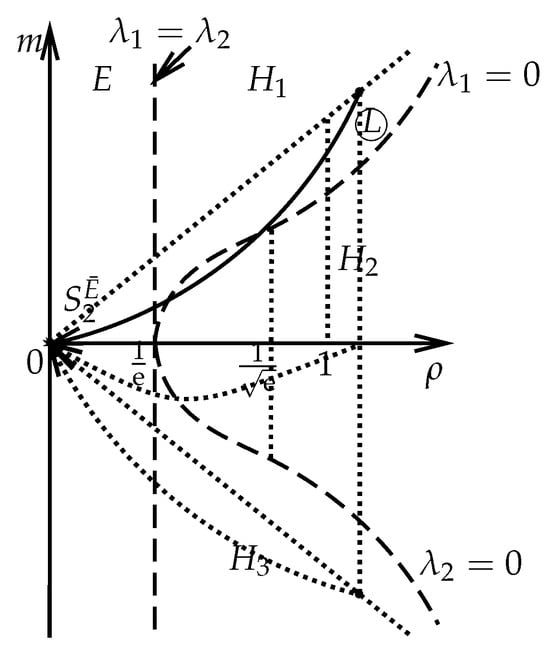
Figure 9. The second family shock wave $S_2^{\overline{E}}$ if the left state $({\rho }_l,m_l)$ is in the hyperbolic region, while the right state can be in the hyperbolic region or in the elliptic region.

In Figure 9, the dotted curves denote the $S_2^{\overline{E}}$ from the left state $({\rho }_l,u_l)$ in the different hyperbolic region to the original point. Along this shock wave $S_2^{\overline{E}}$, we have that

$${\displaystyle \frac{\mathrm{d}}{\mathrm{d}\rho }}\left({\displaystyle \frac{m-m_l}{\rho -{\rho }_l}}\right)={\displaystyle \frac{G^{\prime }\left(\rho \right)}{2\sqrt{{\rho }_{l}G\left(\rho \right)}}}>0.$$

(50)

Based on the above analysis, we know that for Case I, the wave is the first family shock wave which is in the hyperbolic region. For Case II, the wave is also the first family shock wave, while it is not connected. For case III, the wave is the second family shock wave which is in the hyperbolic region. For case IV, the wave is the second family shock wave, while it is not connected. In fact, for case III and case IV, the two shock waves form a continuity curve for the same left state.

Remark 2.

We illustrate that the notations S, $S^E$, and $S^{\overline{E}}$ all denote the shock waves. But there is a little difference. If both the left state and right state are in the hyperbolic region, the shock wave is marked S. If one of the two states is in the hyperbolic region and the other one is in the elliptic region, the shock wave is marked $S^E$. If one of the states is in the hyperbolic region and the other state can be in both regions, the shock wave is marked $S^{\overline{E}}$. For example, for Case III, the shock wave is $S_2$. For Case IV, the shock wave is $S_2^E$. Then, it holds that $S_2^{\overline{E}}=S_2\cup S_2^E$.

4. Rarefaction Waves

A rarefaction wave is a continuous solution of (1) of form $(\rho ,u)\left(\xi \right)$, $\xi ={\displaystyle \frac{x}{t}}$. The k-rarefaction wave curves are the sets of states that are connected to $({\rho }_l,m_l)$, which means that the k-Riemann invariants ${\omega }_k$ are constants, $k=1,2$. Then, we obtain the equations of the 1-rarefaction wave denoted by $R_1$ and 2-rarefaction wave denoted by $R_2$ (see Figure 10). In Figure 10, the dotted curves denote $R_1$ from $({\rho }_l,m_l)$ to the boundary of the elliptic region and $R_2$ from $({\rho }_l,m_l)$ to infinity.

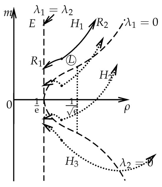
Figure 10. The rarefaction waves $R_1$ and $R_2$ if the left state $({\rho }_l,m_l)$ is in the hyperbolic region H.

The 1-rarefaction wave $R_1$ satisfies

$$R_1({\rho }_l,m_l):\left\{\begin{array}{c}m-m_l={\displaystyle \frac{m_l}{{\rho }_l}}(\rho -{\rho }_l)-{\displaystyle \frac{2}{3}}\rho \left({(ln\rho +1)}^{{\displaystyle \frac{3}{2}}}-{(ln{\rho }_l+1)}^{{\displaystyle \frac{3}{2}}}\right),{\rho }_l>\rho >{\displaystyle \frac{1}{\mathrm{e}}},\hfill \\ \xi =u-\sqrt{ln\rho +1}.\hfill \end{array}\right.$$

(51)

Along the $R_1$, we have that

$$\left\{\begin{array}{c}{\displaystyle \frac{\mathrm{d}m}{\mathrm{d}\rho }}={\displaystyle \frac{m_l}{{\rho }_l}}-{\displaystyle \frac{2}{3}}\left({(ln\rho +1)}^{{\displaystyle \frac{3}{2}}}-{(ln{\rho }_l+1)}^{{\displaystyle \frac{3}{2}}}\right)-\sqrt{ln\rho +1}={\lambda }_1(\rho ,u),\hfill \\ {\displaystyle \frac{{\mathrm{d}}^{2}m}{\mathrm{d}{\rho }^2}}=-{\displaystyle \frac{\sqrt{ln\rho +1}}{\rho }}-{\displaystyle \frac{1}{2\rho \sqrt{ln\rho +1}}}<0.\hfill \end{array}\right.$$

(52)

The 2-rarefaction wave $R_2$ satisfies

$$R_2({\rho }_l,m_l):\left\{\begin{array}{c}m-m_l={\displaystyle \frac{m_l}{{\rho }_l}}(\rho -{\rho }_l)+{\displaystyle \frac{2}{3}}\rho \left({(ln\rho +1)}^{{\displaystyle \frac{3}{2}}}-{(ln{\rho }_l+1)}^{{\displaystyle \frac{3}{2}}}\right),\rho >{\rho }_l>{\displaystyle \frac{1}{\mathrm{e}}},\hfill \\ \xi =u+\sqrt{ln\rho +1}.\hfill \end{array}\right.$$

(53)

Along the $R_2$, we have that

$$\left\{\begin{array}{c}{\displaystyle \frac{\mathrm{d}m}{\mathrm{d}\rho }}={\displaystyle \frac{m_l}{{\rho }_l}}+{\displaystyle \frac{2}{3}}\left({(ln\rho +1)}^{{\displaystyle \frac{3}{2}}}-{(ln{\rho }_l+1)}^{{\displaystyle \frac{3}{2}}}\right)+\sqrt{ln\rho +1}={\lambda }_2(\rho ,u),\hfill \\ {\displaystyle \frac{{\mathrm{d}}^{2}m}{\mathrm{d}{\rho }^2}}={\displaystyle \frac{\sqrt{ln\rho +1}}{\rho }}+{\displaystyle \frac{1}{2\rho \sqrt{ln\rho +1}}}>0.\hfill \end{array}\right.$$

(54)

5. Riemann Solutions

In this section, we construct the Riemann solution for the mixed-type model (1) and (2) with the initial data (5). For the fixed left state $({\rho }_l,m_l)$, we divide the $(\rho ,m)$ plane into several regions by the shock waves in Section 3 and the rarefaction waves in Section 4. In the following, we will analyze two cases, where the left states are in the elliptic region ($0<{\rho }_l<{\displaystyle \frac{1}{\mathrm{e}}}$) and hyperbolic region (${\rho }_l\ge {\displaystyle \frac{1}{\mathrm{e}}}$), respectively.

Case 1. Assuming that $({\rho }_l,u_l)$ is in the elliptic region, that is, $0<{\rho }_l<{\displaystyle \frac{1}{\mathrm{e}}}$, we construct the Riemann solutions for the right state in the solvable regions I and $II$, as in Figure 11. The boundaries of region I are $R_2({\rho }_l^{\ast },m_l^{\ast })$ and $S_1^E({\rho }_l,m_l)$ with $\rho >{\rho }_l^{\ast }$. The boundaries of region $II$ are $S_1^E({\rho }_l,m_l)$, $S_2({\rho }_l^{\ast },m_l^{\ast })$, $S_2^E({\rho }_l^{\ast },m_l^{\ast })$, $\mathsf{\Gamma }$ and the negative axis of m, where $\mathsf{\Gamma }$ satisfies

$$\begin{array}{cc}\hfill \left\{\right(\rho ,m\left)\right|m=& {\displaystyle \frac{m^{\ast }}{{\rho }^{\ast }}}\rho ,m^{\ast }={\displaystyle \frac{m_l}{{\rho }_l}}{\rho }^{\ast }-({\rho }^{\ast }-{\rho }_l)\sqrt{{\displaystyle \frac{{\rho }^{\ast }\left({\rho }^{\ast }ln{\rho }^{\ast }-{\rho }_{l}ln{\rho }_l\right)}{{\rho }_l\left({\rho }^{\ast }-{\rho }_l\right)}}},{\rho }_l^{\ast }<{\rho }^{\ast }<1,\hfill \\ \hfill & \rho ln\rho ={\rho }^{\ast }ln{\rho }^{\ast },0<\rho <{\rho }_l\}.\hfill \end{array}$$

(55)

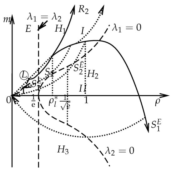
Figure 11. The left state $({\rho }_l,m_l)$ is in the elliptic region and the right state is in region I or $II$.

If the right states $({\rho }_r,m_r)$ are located in the region of I, then the solution is constructed as

$$({\rho }_l,m_l)\stackrel{S_1^E}{\to }({\rho }_1,m_1)\stackrel{R_2}{\to }({\rho }_r,m_r),$$

(56)

where $({\rho }_1,m_1)$ satisfy

$$\left\{\begin{array}{c}{\displaystyle \frac{m_1-m_l}{{\rho }_1-{\rho }_l}}={\displaystyle \frac{m_l}{{\rho }_l}}-\sqrt{{\displaystyle \frac{{\rho }_1\left({\rho }_{1}ln{\rho }_1-{\rho }_{l}ln{\rho }_l\right)}{{\rho }_l\left({\rho }_1-{\rho }_l\right)}}},\hfill \\ m_r-m_1={\displaystyle \frac{m_1}{{\rho }_1}}({\rho }_r-{\rho }_1)+{\displaystyle \frac{2}{3}}{\rho }_r\left({(ln{\rho }_r+1)}^{{\displaystyle \frac{3}{2}}}-{(ln{\rho }_1+1)}^{{\displaystyle \frac{3}{2}}}\right).\hfill \end{array}\right.$$

(57)

If the right states $({\rho }_r,m_r)$ are located in the region of $II$, then the solution is constructed as

$$({\rho }_l,m_l)\stackrel{S_1^E}{\to }({\rho }_1,m_1)\stackrel{S_2\mathrm{or}{S}_2^E\mathrm{or}{S}_2^{\overline{E}}}{\to }({\rho }_r,m_r),$$

(58)

where $({\rho }_1,m_1)$ satisfy

$$\left\{\begin{array}{c}{\displaystyle \frac{m_1-m_l}{{\rho }_1-{\rho }_l}}={\displaystyle \frac{m_l}{{\rho }_l}}-\sqrt{{\displaystyle \frac{{\rho }_1\left({\rho }_{1}ln{\rho }_1-{\rho }_{l}ln{\rho }_l\right)}{{\rho }_l\left({\rho }_1-{\rho }_l\right)}}},\hfill \\ {\displaystyle \frac{m_r-m_1}{{\rho }_r-{\rho }_1}}={\displaystyle \frac{m_1}{{\rho }_1}}+\sqrt{{\displaystyle \frac{{\rho }_r\left({\rho }_{r}ln{\rho }_r-{\rho }_{1}ln{\rho }_1\right)}{{\rho }_1\left({\rho }_r-{\rho }_1\right)}}}.\hfill \end{array}\right.$$

(59)

Case 2. Assuming that the $({\rho }_l,u_l)$ is in the hyperbolic region of $H_1=\{(\rho ,m)|\rho >{\displaystyle \frac{1}{\mathrm{e}}},0<{\lambda }_1<{\lambda }_2\}$, we construct the Riemann solutions for the right state in different regions. There are two subcases.

Subcase 2.1. ${\displaystyle \frac{1}{\mathrm{e}}}\le {\rho }_l\le 1$. We construct the Riemann solutions for the right state in the solvable regions $I^{\prime }$, $I{I}^{\prime }$, $II{I}^{\prime }$, and $I{V}^{\prime }$, as in Figure 12. The boundaries of $I^{\prime }$ are $R_2({\rho }_l,m_l)$ and $S_1({\rho }_l,m_l)$ with $\rho >{\rho }_l$. The boundaries of $I{I}^{\prime }$ are $R_1({\rho }_l,m_l)$, $R_2({\rho }_l,m_l)$, and $R_2({\displaystyle \frac{1}{\mathrm{e}}},m_e)$, where $({\displaystyle \frac{1}{\mathrm{e}}},m_e)$ is on the curve $R_1({\rho }_l,m_l)$. The boundaries of $II{I}^{\prime }$ are $R_1({\rho }_l,m_l)$, $S_2({\rho }_l,m_l)$, $S_2^E({\rho }_l,m_l)$ and ${\mathsf{\Gamma }}_1$, where ${\mathsf{\Gamma }}_1$ satisfies

$$\begin{array}{cc}\hfill \left\{\right(\rho ,m\left)\right|& m={\displaystyle \frac{m^{\ast }}{{\rho }^{\ast }}}\rho ,m^{\ast }={\displaystyle \frac{m_l}{{\rho }_l}}{\rho }^{\ast }-{\displaystyle \frac{2}{3}}{\rho }^{\ast }\left({(ln{\rho }^{\ast }+1)}^{{\displaystyle \frac{3}{2}}}-{(ln{\rho }_l+1)}^{{\displaystyle \frac{3}{2}}}\right),{\displaystyle \frac{1}{\mathrm{e}}}<{\rho }^{\ast }<{\rho }_l,\hfill \\ \hfill & \rho ln\rho ={\rho }^{\ast }ln{\rho }^{\ast }\}.\hfill \end{array}$$

(60)

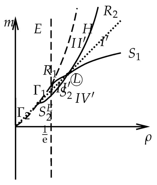
Figure 12. The left state $({\rho }_l,m_l)$ is in the hyperbolic region for ${\displaystyle \frac{1}{\mathrm{e}}}\le {\rho }_l\le 1$, and the right state is in region $I^{\prime }$, $I{I}^{\prime }$, $II{I}^{\prime }$, or $I{V}^{\prime }$.

The boundaries of $I{V}^{\prime }$ are $S_1({\rho }_l,m_l)$, $S_2({\rho }_l,m_l)$, $S_2^E({\rho }_l,m_l)$, ${\mathsf{\Gamma }}_2$ and the negative axis of m, where ${\mathsf{\Gamma }}_2$ satisfies

$$\begin{array}{cc}\hfill \left\{\right(\rho ,m\left)\right|m=& {\displaystyle \frac{m^{\ast }}{{\rho }^{\ast }}}\rho ,m^{\ast }={\displaystyle \frac{m_l}{{\rho }_l}}{\rho }^{\ast }-({\rho }^{\ast }-{\rho }_l)\sqrt{{\displaystyle \frac{{\rho }^{\ast }\left({\rho }^{\ast }ln{\rho }^{\ast }-{\rho }_{l}ln{\rho }_l\right)}{{\rho }_l\left({\rho }^{\ast }-{\rho }_l\right)}}},\hfill \\ \hfill & \rho ln\rho ={\rho }^{\ast }ln{\rho }^{\ast },0<\rho <{\rho }_l^{\ast }\}.\hfill \end{array}$$

(61)

If the right states $({\rho }_r,m_r)$ are located in the region of $I^{\prime }$, then the solution is constructed as

$$({\rho }_l,m_l)\stackrel{S_1}{\to }({\rho }_1,m_1)\stackrel{R_2}{\to }({\rho }_r,m_r),$$

(62)

where $({\rho }_1,m_1)$ satisfy

$$\left\{\begin{array}{c}{\displaystyle \frac{m_1-m_l}{{\rho }_1-{\rho }_l}}={\displaystyle \frac{m_l}{{\rho }_l}}-\sqrt{{\displaystyle \frac{{\rho }_1\left({\rho }_{1}ln{\rho }_1-{\rho }_{l}ln{\rho }_l\right)}{{\rho }_l\left({\rho }_1-{\rho }_l\right)}}},\hfill \\ m_r-m_1={\displaystyle \frac{m_1}{{\rho }_1}}({\rho }_r-{\rho }_1)+{\displaystyle \frac{2}{3}}{\rho }_r\left({(ln{\rho }_r+1)}^{{\displaystyle \frac{3}{2}}}-{(ln{\rho }_1+1)}^{{\displaystyle \frac{3}{2}}}\right).\hfill \end{array}\right.$$

(63)

If the right states $({\rho }_r,m_r)$ are located in the region of $I{I}^{\prime }$, then the solution is constructed as

$$({\rho }_l,m_l)\stackrel{R_1}{\to }({\rho }_1,m_1)\stackrel{R_2}{\to }({\rho }_r,m_r),$$

(64)

where $({\rho }_1,m_1)$ satisfy

$$\left\{\begin{array}{c}{m}_1-m_l={\displaystyle \frac{m_l}{{\rho }_l}}({\rho }_1-{\rho }_l)-{\displaystyle \frac{2}{3}}{\rho }_1\left({(ln{\rho }_1+1)}^{{\displaystyle \frac{3}{2}}}-{(ln{\rho }_l+1)}^{{\displaystyle \frac{3}{2}}}\right),\hfill \\ m_r-m_1={\displaystyle \frac{m_1}{{\rho }_1}}({\rho }_r-{\rho }_1)+{\displaystyle \frac{2}{3}}{\rho }_r\left({(ln{\rho }_r+1)}^{{\displaystyle \frac{3}{2}}}-{(ln{\rho }_1+1)}^{{\displaystyle \frac{3}{2}}}\right).\hfill \end{array}\right.$$

(65)

Similar to case 1, the solution may also be constructed as

$$({\rho }_l,m_l)\stackrel{S_2}{\to }({\rho }_1,m_1)\stackrel{R_2}{\to }({\rho }_r,m_r).$$

(66)

If the right states $({\rho }_r,m_r)$ are located in the region of $II{I}^{\prime }$, then the solution is constructed as

$$({\rho }_l,m_l)\stackrel{R_1}{\to }({\rho }_1,m_1)\stackrel{S_2\mathrm{or}{S}_2^E}{\to }({\rho }_r,m_r),$$

(67)

where $({\rho }_1,m_1)$ satisfy

$$\left\{\begin{array}{c}{m}_1-m_l={\displaystyle \frac{m_l}{{\rho }_l}}({\rho }_1-{\rho }_l)-{\displaystyle \frac{2}{3}}{\rho }_1\left({(ln{\rho }_1+1)}^{{\displaystyle \frac{3}{2}}}-{(ln{\rho }_l+1)}^{{\displaystyle \frac{3}{2}}}\right),\hfill \\ {\displaystyle \frac{m_r-m_1}{{\rho }_r-{\rho }_1}}={\displaystyle \frac{m_1}{{\rho }_1}}+\sqrt{{\displaystyle \frac{{\rho }_r\left({\rho }_{r}ln{\rho }_r-{\rho }_{1}ln{\rho }_1\right)}{{\rho }_1\left({\rho }_r-{\rho }_1\right)}}}.\hfill \end{array}\right.$$

(68)

If the right states $({\rho }_r,m_r)$ are located in the region of $I{V}^{\prime }$, then the solution is constructed as

$$({\rho }_l,m_l)\stackrel{S_1}{\to }({\rho }_1,m_1)\stackrel{S_2\mathrm{or}{S}_2^E}{\to }({\rho }_r,m_r),$$

(69)

where $({\rho }_1,m_1)$ satisfy

$$\left\{\begin{array}{c}{\displaystyle \frac{m_1-m_l}{{\rho }_1-{\rho }_l}}={\displaystyle \frac{m_l}{{\rho }_l}}-\sqrt{{\displaystyle \frac{{\rho }_1\left({\rho }_{1}ln{\rho }_1-{\rho }_{l}ln{\rho }_l\right)}{{\rho }_l\left({\rho }_1-{\rho }_l\right)}}},\hfill \\ {\displaystyle \frac{m_r-m_1}{{\rho }_r-{\rho }_1}}={\displaystyle \frac{m_1}{{\rho }_1}}+\sqrt{{\displaystyle \frac{{\rho }_r\left({\rho }_{r}ln{\rho }_r-{\rho }_{1}ln{\rho }_1\right)}{{\rho }_1\left({\rho }_r-{\rho }_1\right)}}}.\hfill \end{array}\right.$$

(70)

Subcase 2.2. ${\rho }_l\ge 1$. We construct the Riemann solutions for the right state in the solvable regions $I^{″}$, $I{I}^{″}$, $II{I}^{″}$, and $I{V}^{″}$, as in Figure 13. The boundaries of $I^{″}$ are $R_2({\rho }_l,m_l)$ and $S_1({\rho }_l,m_l)$ with $\rho >{\rho }_l$. The boundaries of $I{I}^{″}$ are $R_1({\rho }_l,m_l)$, $R_2({\rho }_l,m_l)$, and $R_2({\displaystyle \frac{1}{\mathrm{e}}},m_e)$, where $({\displaystyle \frac{1}{\mathrm{e}}},m_e)$ is on the curve $R_1({\rho }_l,m_l)$. The boundaries of $II{I}^{″}$ are $R_1({\rho }_l,m_l)$, $S_2^{\overline{E}}({\rho }_l,m_l)$, and $\overline{\mathsf{\Gamma }}$, where $\overline{\mathsf{\Gamma }}$ satisfies

$$\begin{array}{cc}\hfill \left\{\right(\rho ,m\left)\right|& m={\displaystyle \frac{m^{\ast }}{{\rho }^{\ast }}}\rho ,m^{\ast }={\displaystyle \frac{m_l}{{\rho }_l}}{\rho }^{\ast }-{\displaystyle \frac{2}{3}}{\rho }^{\ast }\left({(ln{\rho }^{\ast }+1)}^{{\displaystyle \frac{3}{2}}}-{(ln{\rho }_l+1)}^{{\displaystyle \frac{3}{2}}}\right),\hfill \\ \hfill & \rho ln\rho ={\rho }^{\ast }ln{\rho }^{\ast },{\displaystyle \frac{1}{\mathrm{e}}}<{\rho }^{\ast }<1\}.\hfill \end{array}$$

(71)

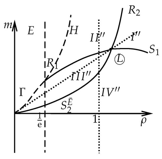
Figure 13. The left state $({\rho }_l,m_l)$ is in the hyperbolic region for ${\rho }_l\ge 1$, and the right state is in region $I^{\prime \prime }$, $I{I}^{″}$, $II{I}^{\prime \prime }$, or $I{V}^{\prime \prime }$.

The boundaries of $I{V}^{″}$ are $S_2^{\overline{E}}({\rho }_l,m_l)$ and $S_1({\rho }_l,m_l)$.

If the right states $({\rho }_r,m_r)$ are located in the region of $I^{″}$, then the solution is constructed as (62). If the right states $({\rho }_r,m_r)$ are located in the region of $I{I}^{″}$, then the solution is constructed as (64). If the right states $({\rho }_r,m_r)$ are located in the region of $II{I}^{″}$, then the solution is constructed as (67). If the right states $({\rho }_r,m_r)$ are located in the region of $I{V}^{″}$, then the solution is constructed as

$$({\rho }_l,m_l)\stackrel{S_1}{\to }({\rho }_1,m_1)\stackrel{S_2^{\overline{E}}}{\to }({\rho }_r,m_r),$$

(72)

where $({\rho }_1,m_1)$ satisfy

$$\left\{\begin{array}{c}{\displaystyle \frac{m_1-m_l}{{\rho }_1-{\rho }_l}}={\displaystyle \frac{m_l}{{\rho }_l}}-\sqrt{{\displaystyle \frac{{\rho }_1\left({\rho }_{1}ln{\rho }_1-{\rho }_{l}ln{\rho }_l\right)}{{\rho }_l\left({\rho }_1-{\rho }_l\right)}}},\hfill \\ {\displaystyle \frac{m_r-m_1}{{\rho }_r-{\rho }_1}}={\displaystyle \frac{m_1}{{\rho }_1}}+\sqrt{{\displaystyle \frac{{\rho }_r\left({\rho }_{r}ln{\rho }_r-{\rho }_{1}ln{\rho }_1\right)}{{\rho }_1\left({\rho }_r-{\rho }_1\right)}}}.\hfill \end{array}\right.$$

(73)

Similarly, if the left state is in the hyperbolic region of $H_2$ or $H_3$ with ${\rho }_l>1$, the unique Riemann solution can be also constructed. We omit them. In conclusion, we have the following result.

Theorem 1.

For the fixed left states $({\rho }_l,u_l)$ and the right states $({\rho }_r,u_r)$ in the feasible regions as described in cases 1 and 2 (see Figure 11, Figure 12 and Figure 13), the Riemann problems (1), (2), and (5) have a unique weak solution satisfying the entropy condition (32).

6. Numerical Tests

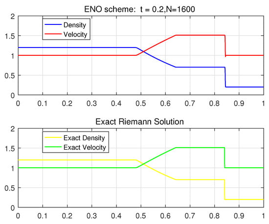
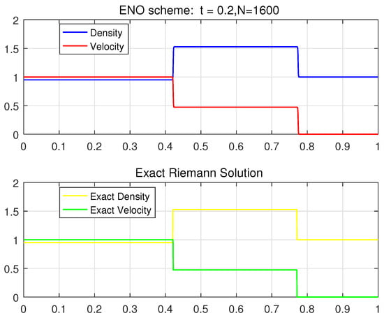
In this section, we present some numerical tests to verify our theoretical results for the construction of the Riemann solutions for (1) and (2) with initial data (5). We use the essentially non-oscillatory (ENO) scheme [40] and third-order Runge–Kutta method with 60 × 60 cells. The $CFL=0.4$ and the running time $T=0.2$. Many more numerical tests have been performed to make sure that what are presented are not numerical artifacts. Here, we present three cases to verify our theoretical solution.

Case 1. In this case, we take the initial Riemann data as

$$\left(\rho ,u\right){|}_{t=0}=\left\{\begin{array}{cc}(1.2,1)\hfill & x<0,\hfill \\ (0.2,1)\hfill & x>0,\hfill \end{array}\right.$$

(74)

where the left state $(1.2,1)$ belongs to the hyperbolic region and the right state $(0.2,1)$ belongs to the elliptic region.

As marked in Figure 14, Figure 15 and Figure 16, the red and blue lines in the upper half plane represent approximate density and velocity, and the yellow and green lines in the lower half plane represent the exact density and velocity, respectively. From Figure 14, we find that the left state of (74) is connected to the intermediate state by a rarefaction wave, and then to the right state of (74) by a shock wave. This verifies the theoretical solution for Subcase 2.2 in Section 5 in which the right state is located in region $II{I}^{″}$ of the left state.

Figure 14. Riemann solution for (1), (2), and (74). The left state is in the hyperbolic region, and the right state is in the elliptic region.

Figure 15. Riemann solution for (1), (2), and (75). The left state is in the elliptic region, and the right state is in the hyperbolic region.

Figure 16. Riemann solution for (1), (2), and (76). Both of the initial states are in the hyperbolic region.

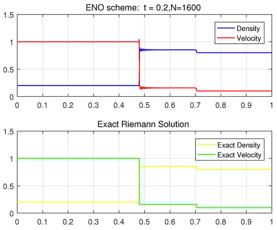
Case 2. In this case, we take the initial Riemann data as

$$\left(\rho ,u\right){|}_{t=0}=\left\{\begin{array}{cc}(0.2,1)\hfill & x<0,\hfill \\ (0.8,0.1)\hfill & x>0,\hfill \end{array}\right.$$

(75)

where the left state $(0.2,1)$ belongs to the elliptic region and the right state $(0.8,0.1)$ belongs to the hyperbolic region. From Figure 15, the Riemann solution consists of three constant states separated by two shock waves. Specifically, the left state of (75) is connected to the intermediate state by a shock wave, and then to the right state of (75) by a shock wave. This verifies the theoretical solution for Case 1 in Section 5 in which the right state is located in region $II$ of the left state.

Case 3. In this case, we take the initial Riemann data as

$$\left(\rho ,u\right){|}_{t=0}=\left\{\begin{array}{cc}(0.95,1)\hfill & x<0,\hfill \\ (1,0)\hfill & x>0,\hfill \end{array}\right.$$

(76)

where both the left state $(0.95,1)$ and the right state $(1,0)$ are in the hyperbolic region. From Figure 16, the Riemann solution also consists of three constant states separated by two shock waves. This verifies the theoretical solution for Subcase 2.1 in Section 5 in which the right state is located in region $I{V}^{\prime }$ of the left state.

It is worth pointing out that the Gibbs phenomenon [38] appears in Cases 1 and 2, where one of the initial state is in the hyperbolic region, and the other state is in the elliptic region, while in Case 3, where both of the initial states are in the hyperbolic region, the Gibbs phenomenon does not appear. It inspires us to find a better numerical scheme to capture the shock wave in the mixed conservation laws in our further works.

7. Discussion

The shape of the elliptic regions (1) with (2) and the van der Waals models [21] forms a strip. However, for systems (1) and (2), there is one hyperbolic region, while there are two hyperbolic regions for van der Waals, whose nonclassical shocks satisfy a kinetic relation [23]. This difference implies that methods applicable to the study of the van der Waals models are not suitable for systems (1) and (2). Furthermore, in the previous studies [29,30,31,34], we observe that the challenges in studying mixed-type partial differential equations are contingent upon the shape of the elliptic regions.

From the previous models [29,30,39,41], the uniqueness of the solution of the hyperbolic–elliptic model could not be obtained by the Lax entropy condition or the Liu entropy condition. For our models (1) and (2), the Hugoniot curves (13) are not connected or self-intersecting (see Figure 3). We provide the entropy condition (32) to pick up the admissible shock waves, including the elliptic region.

In this paper, the feasible regions are contained in Figure 11, Figure 12 and Figure 13. For the ideal gas or Chaplygin gas, the systems are hyperbolic. For these models, a vacuum or a delta shock wave exists in the intractable regions, in which the Riemann solution cannot be constructed by the shock waves and rarefaction waves [15,37]. However, the dark energy fluid (1) with (2) is of mixed type. The methods for investigating the two systems are different. In our work, there exist intractable regions in each case. This singularity may result in a vacuum, a delta shock wave, or other types of singularities. This problem is worth further study.

8. Conclusions

In this paper, we construct the Riemann solutions for the mixed-type isentropic Euler Equations (1), in which the pressure (2) is a special case of the generalized dark energy EoS (3). Using the Rankine–Hugoniot conditions for the mixed-type systems (1) and (2), we find that the discontinuity curves may exist in both elliptic regions and hyperbolic regions. The classical entropy condition is not applicable. We obtain the unique admissible shock waves by utilizing the viscosity criterion. The principal element in the construction is a division of the $(\rho ,m)$-plane into several regions, the division depending upon the location of $({\rho }_l,m_l)$. The solution of the Riemann problem consists of a combination of admissible shock waves and rarefaction waves, the combination determined by the region in which $({\rho }_r,m_r)$ lies. Finally, we present numerical simulations which are consistent with our theoretical results.

References

- Diperna, R. Convergence of viscosity method for isentropic gas dynamics. Commun. Math. Phys. 1983, 91, 1–30. [Google Scholar] [CrossRef]
- Oikonomou, V.K. Generalized Logarithmic equation of state in classical and loop quantum cosmology dark energy-dark matter coupled systems. Ann. Phys. 2019, 409, 167934. [Google Scholar] [CrossRef]
- Pan, S.; Yang, W.; Di Valentino, E.; Saridakis, E.N.; Chakraborty, S. Interacting scenarios with dynamical dark energy: Observational constraints and alleviation of the H0 tension. Phys. Rev. D 2019, 100, 103520. [Google Scholar] [CrossRef]
- Mayer, B.; Anton, H.; Bott, E.; Methfessel, M.; Sticht, J.; Harris, J.; Schmidt, P.C. Ab-initio calculation of the elastic constants and thermal expansion coefficients of Laves phases. Intermetallics 2003, 11, 23–32. [Google Scholar] [CrossRef]
- Chen, G.Q. The Theory of Compensated Compactness and the System of Isentropic Gas Dynamics; Math Sciences Research Institute: Berkeley, CA, USA, 1990; Preprint 00527-91. [Google Scholar]
- Chen, G.Q.; Le Floch, P. Compressible Euler equations with general pressure law. Arch. Ration. Mech. Anal. 2000, 153, 221–259. [Google Scholar] [CrossRef]
- Chen, G.Q.; Huang, F.M.; Wang, T.Y. Isothermal limit of entropy solutions of the Euler equations for isentropic gas dynamics. SIAM J. Math. Anal. 2024, 56, 1300–1320. [Google Scholar] [CrossRef]
- Ding, X.Q.; Chen, G.Q.; Luo, P.Z. Convergence of the Lax-Friedrichs scheme for isentropic gas dynamics (I). Acta Math. Sci. (Engl. Ed.) 1985, 5, 415–432. [Google Scholar] [CrossRef]
- Ding, X.Q.; Chen, G.Q.; Luo, P.Z. Convergence of the Lax-Friedrichs scheme for isentropic gas dynamics (II). Acta Math. Sci. (Engl. Ed.) 1985, 5, 433–472. [Google Scholar] [CrossRef]
- Huang, F.M.; Wang, Z. Convergence of viscosity solutions for isothermal gas dynamics. SIAM J. Math. Anal. 2002, 34, 595–610. [Google Scholar] [CrossRef]
- Lions, P.L.; Perthame, B.; Tadmor, E. Kinetic formulation of the isentropic gas dynamics and p-systems. Commun. Math. Phys. 1994, 163, 169–172. [Google Scholar] [CrossRef]
- Lions, P.L.; Perthame, B.; Souganidis, P. Existence and stability of entropy solutions for the hyperbolic systems of isentropic gas dynamics in Eulerian and Lagrangian coordinates. Commun. Pure Appl. Math. 1996, 49, 599–638. [Google Scholar] [CrossRef]
- Lu, Y.G. Existence of global entropy solutions to a nonstrictly hyperbolic system. Arch. Ration. Mech. Anal. 2005, 178, 287–299. [Google Scholar] [CrossRef]
- Shah, S.; Singh, R.; Jena, J. Steepened wave in two-phase Chaplygin flows comprising a source term. Appl. Math. Comput. 2022, 413, 126656. [Google Scholar] [CrossRef]
- Brenier, Y. Solutions with concentration to the Riemann problem for the one-dimensional Chaplygin gas equations. J. Math. Fluid Mech. 2005, 7, S326–S331. [Google Scholar] [CrossRef]
- Sun, M. Concentration and cavitation phenomena of Riemann solutions for the isentropic Euler system with the logarithmic equation of state. Nonlinear Anal. Real World Appl. 2020, 53, 103068. [Google Scholar] [CrossRef]
- Chavanis, P.H. The Logotropic dark fluid as a unification of dark matter and dark energy. Phys. Lett. B 2016, 758, 59–66. [Google Scholar] [CrossRef]
- Evans, L.C. Partial Differential Equations, 2nd ed.; American Mathematical Society: Providence, RI, USA, 2010; pp. xxii+749. [Google Scholar]
- Mercier, J.M.; Piccoli, B. Admissible Riemann solvers for genuinely nonlinear p-systems of mixed type. J. Differ. Equ. 2002, 80, 395–426. [Google Scholar] [CrossRef]
- Fan, H.; Slemrod, M. The Riemann problem for systems of conservation laws of mixed type. In Shock Induced Transitions and Phase Structures in General Media; The IMA Volumes in Mathematics and its Applications; Springer: New York, NY, USA, 1993; Volume 52, pp. 61–69. [Google Scholar]
- Slemrod, M. Admissibility criteria for propagating phase boundaries in a van der Waals fluid. Arch. Rational Mech. Anal. 1983, 81, 301–315. [Google Scholar] [CrossRef]
- Shearer, M. The Riemann problem for a class of conservation laws of mixed type. J. Differ. Equ. 1982, 46, 426–443. [Google Scholar] [CrossRef]
- Thanh, M.D.; Vinh, D.X. The Riemann problem for van der Waals fluids with nonclassical phase transitions. Hokkaido Math. J. 2021, 50, 263–295. [Google Scholar] [CrossRef]
- Lax, P.D. Hyperbolic systems of conservation laws. Commun. Pure Appl. Math. 1957, 10, 537–566. [Google Scholar] [CrossRef]
- Liu, T.P. The Riemann problem for general system of conservation laws. J. Differ. Equ. 1975, 18, 218–234. [Google Scholar] [CrossRef]
- Azevedo, A.V.; Marchesin, D. Multiple viscous profile Riemann solutions in mixed elliptic-hyperbolic models for flow in porous media. In Nonlinear Evolution Equations that Change Type; The IMA Volumes in Mathematics and its Applications; Springer: New York, NY, USA, 1990; Volume 27, pp. 1–17. [Google Scholar]
- Azevedo, A.V.; Marchesin, D.; Plohr, B.; Zumbrun, K. Capillary instability in models for three-phase flow. Z. Angew. Math. Phys. 2002, 53, 713–746. [Google Scholar] [CrossRef]
- Chalons, C.; Coquel, F.; Engel, P.; Rohde, C. Fast relaxation solvers for hyperbolic-elliptic phase transition problems. SIAM J. Sci. Comput. 2012, 34, A1753–A1776. [Google Scholar] [CrossRef][Green Version]
- He, F.; Wang, Z.; Chen, T. The Shock Waves for a Mixed-Type System from Chemotaxis. Acta Math. Sci. Ser. B (Engl. Ed.) 2023, 43, 1717–1734. [Google Scholar] [CrossRef]
- Holden, H. On the Riemann problem for a prototype of a mixed type conservation law. Commun. Pure Appl. Math. 1987, 40, 229–264. [Google Scholar] [CrossRef]
- Hsiao, L.; De Mottoni, P. Existence and uniqueness of the Riemann problem for a nonlinear system of conservation laws of mixed type. Trans. Am. Math. Soc. 1990, 322, 121–158. [Google Scholar] [CrossRef]
- Keyfitz, B.L.; Sanders, R.; Sever, M. Lack of hyperbolicity in the two-fluid model for two-phase incompressible flow. Discret. Contin. Dyn. Syst. Ser. B 2003, 3, 541–563. [Google Scholar] [CrossRef]
- Li, T.; Liu, H.; Wang, L. Oscillatory traveling wave solutions to an attractive chemotaxis system. J. Differ. Equ. 2016, 261, 7080–7098. [Google Scholar] [CrossRef]
- Li, T.; Mathur, N. Riemann problem for a non-srtrictly hyperbolic system in chemotaxis. Discret. Contin. Dyn. Syst. Ser. B 2022, 27, 2173–2187. [Google Scholar] [CrossRef]
- Mailybaev, A.A.; Marchesin, D. Lax shocks in mixed-type systems of conservation laws. J. Hyperbolic Differ. Equ. 2008, 5, 295–315. [Google Scholar] [CrossRef]
- Medeiros, H.B. Stable hyperbolic singularities for three-phase flow models in oil reservoir simulation. Acta Appl. Math. 1992, 28, 135–159. [Google Scholar] [CrossRef]
- Smoller, J. Shock Waves and Reaction-Diffusion Equations, 2nd ed.; Springer: New York, NY, USA, 1994. [Google Scholar]
- Gottlieb, D.; Shu, C.W. On the Gibbs phenomenon and its resolution. SIAM Rev. 1997, 39, 644–668. [Google Scholar] [CrossRef]
- Hsiao, L. Uniqueness of admissibel solutions of Riemann problem of systems of conservation laws of mixed type. J. Differ. Equ. 1990, 86, 197–233. [Google Scholar] [CrossRef]
- Jiang, G.S.; Shu, C.W. Efficient implementation of weighted ENO schemes. J. Comput. Phys. 1996, 126, 202–228. [Google Scholar] [CrossRef]
- Shearer, M. Nonuniqueness of admissible solutions of Riemann initial value problems for a system of conservation laws of mixed type. Arch. Ration. Mech. Anal. 1986, 93, 45–59. [Google Scholar] [CrossRef]
Disclaimer/Publisher’s Note: The statements, opinions and data contained in all publications are solely those of the individual author(s) and contributor(s) and not of MDPI and/or the editor(s). MDPI and/or the editor(s) disclaim responsibility for any injury to people or property resulting from any ideas, methods, instructions or products referred to in the content. |
© 2024 by the authors. Licensee MDPI, Basel, Switzerland. This article is an open access article distributed under the terms and conditions of the Creative Commons Attribution (CC BY) license (https://creativecommons.org/licenses/by/4.0/).