Data-Driven Method for Robust Recovery in 1-Bit Compressive Sensing with the Minimax Concave Penalty

Abstract

With the advent of large-scale data, the demand for information is increasing, which makes signal sampling technology and digital processing methods particularly important. The utilization of 1-bit compressive sensing in sparse recovery has garnered significant attention due to its cost-effectiveness in hardware implementation and storage. In this paper, we first leverage the minimax concave penalty equipped with the least squares to recover a high-dimensional true signal $\mathbf{x}\in {\mathbb{R}}^p$ with k-sparse from n-dimensional 1-bit measurements and discuss the regularization by combing the nonconvex sparsity-inducing penalties. Moreover, we give an analysis of the complexity of the method with minimax concave penalty in certain conditions and derive the general theory for the model equipped with the family of sparsity-inducing nonconvex functions. Then, our approach employs a data-driven Newton-type method with stagewise steps to solve the proposed method. Numerical experiments on the synthesized and real data verify the competitiveness of the proposed method.

1. Introduction

With the advent of big data, people’s demand for signal processing is increasing, which drives the need for simpler signal processing technology. In the past decade or two, compressive sensing (CS), as a high-efficiency tool in signal processing, has garnered a lot of interest. However, classical CS faces substantial computing challenges when dealing with larger-dimensional signals due to storage bottlenecks, high transmission bandwidth requirements, and algorithmic inefficiencies. To mitigate these computing costs, it is often effective to quantize measurements by using a finite number of bits. A quantized signal collection method for high-dimensional sparse data processing and storage is 1-bit compressive sensing [1], which transforms the measurements to a single bit, i.e., $\mathbf{y}=sign\left(A\mathbf{x}\right)$ with $\mathbf{y}\in {\mathbb{R}}^n$, $“sign”$ captures the sign of $A{x}^l\in {\mathbb{R}}^p,d^l\in {\mathbb{R}}^p$, and the element ${\mathbf{y}}_i$ is 1 or −1, ${\mathbf{y}}_i\in \{-1,1\}$, $A\in {\mathbb{R}}^{n\times p}$, $\mathbf{x}\in {\mathbb{R}}^p$, n and p are positive integers. Such 1-bit compressive sensing lowers transmission costs, resulting in a significant decrease for hardware implementation. A 1-bit quantizer only needs the sign of the measurements, and thus, is admissible to nonlinear distortion. Furthermore, 1-bit CS can be used effectively in computation due to the binary measurements. The 1-bit CS is suitable for various fields including wireless sensing network and radar analysis [2,3], and in domains like machine learning research, scientific studies, and industrial application. Researchers need to deal with quantized data for producing portable devices, which are necessary in modern life.

In their pioneering work [1], Boufounos and Baraniuk firstly took into account 1-bit noiseless measurements and studied the ${\ell }_1$-norm optimization problem to recover $\mathbf{x}$ with two constraints $\mathbf{y}\odot A\mathbf{x}\ge {0 \mathrm{and}\parallel \mathbf{x}\parallel }_2=1$, where the sign “≥” represents the element-wise inequality and the Hadamard product is represented by ⊙. Jacques et al. [4] considered ${\ell }_0$-norm instead of ${\ell }_1$-norm to enhance sparsity, and established the binary iterative hard thresholding (BIHT or BIHT-${\ell }_2$) algorithm for 1-bit noisy measurements $\mathbf{y}=sign(A\mathbf{x}+\mathbf{b})$, $\mathbf{b}\in {\mathbb{R}}^n$. Matsumoto et al. [5] studied a noisy version with iterative hard thresholding, where a fraction of the measurements can be flipped. Yan et al. [6] considered sign flips in 1-bit measurements by using an adaptive outlier pursuit (AOP) algorithm that was a modified version of BIHT. Plan et al. [7] discussed a combination between the linear loss $(\mathbf{y},A\mathbf{x})$ and ${\ell }_1$-constraint, just as ${min}_{\mathbf{x}}(\mathbf{y},A\mathbf{x})/n,s.t.{\parallel \mathbf{x}\parallel }_1\le \sqrt{k}$ and ${\parallel \mathbf{x}\parallel }_2\le 1$. Ref. [8] studied the Lagrange optimization of the linear loss and ${\ell }_1$-norm and attained the analysis solution $\underset{{\parallel \mathbf{x}\parallel }_2\le 1}{min}(\mathbf{y},A\mathbf{x})/n+\lambda {\parallel \mathbf{x}\parallel }_1$. Dai et al. [9] considered the one-sided ${\ell }_0$ objective model for the noisy 1-bit CS model. Subsequently, Ref. [10] introduced the pitball loss (it involves both ${\ell }_1$-norm and ${\ell }_2$-norms), and proposed the PBAOP algorithm to decode from binary noisy data. Aiming at solutions with better sparsity, Ref. [11] introduced the nonconvex minimax concave penalty (MCP) with linear loss. Refs. [12,13] extended this to the family of nonconvex sparsity-inducing penalties with analytical solutions. However, Refs. [12,13] did not give the estimation error. Ref. [14] considered projected least squares and proposed the LinProj algorithm to decode unknown signals. Huang et al. [15] studied ${\ell }_1$-regularized least squares to decode from 1-bit noisy compressive measurements, and, respectively, proposed PDASC algorithms. Ref. [16] considered nonconvex least-squares loss with ${\ell }_q$ constrained with a higher sparsity level. To attain the target signal with more sparsity, Ref. [17] used the double sparsity of the unknown signal and the measurement to solve 1-bit CS optimization. The above works use the assumption of a sparse signal. In practice, there are other signals such as the gradient sparse signal or block sparse signal. Hou and Liu [18] studied the L1-TV model to solve signals possessing both element sparse and gradient sparse properties. Zhong et al. [19] proposed total variation minimization in the binary setting. Inspired by [20,21], the family of noncovex sparsity reducing penalties has been shown to enjoy good performance when it approximates ${\ell }_0$-norm in conventional CS. In this paper, we try to study the least squares with minimax concave penalty (MCP) and other nonconvex sparsity-inducing penalties to decode from 1-bit CS measurements.

We end this section by giving the structure of this paper as follows. Section 2 gives some notation and preliminaries. Section 3 proposes the least-squares loss equipped with MCP and other nonconvex sparsity-inducing penalties, and discusses the estimation of the non-asymptotical error and the complexity. It then utilizes a Newton-type algorithm with a data-driven parameter voting rule to implement the proposed approach. In Section 4, experiments on synthetic and real datasets are implemented to verify the superiority of the proposed model, and illustrate the robustness and high efficiency of our method. Section 5 gives a short conclusion.

2. Preliminaries

In our work, the 1-bit CS measurement is generally modeled as [15,22]

$$\mathbf{y}=\mathbf{c}\odot sign(A\mathbf{x}+\mathbf{b}),$$

(1)

where $A\in {\mathbb{R}}^{n\times p}$ is the Gaussian measurement matrix, $\mathbf{x}\in {\mathbb{R}}^p$ is the unknown signal to recover, the measurement $\mathbf{y}\in {\{-1,1\}}^n$, $\mathbf{b}\in {\mathbb{R}}^n$ is the random Gauss noise sampled from $\mathcal{N}(0,{ϵ}^2{I}_n)$ with noise level $ϵ$, $\mathbf{c}\in {\mathbb{R}}^n$ is the sign flip, and ⊙ is the Hadamard product. Due to binary nature of the sign function, (1) is nonlinear, and so it is challenging to decode the unknown signal from the noisy and sign-flipped data.

We then introduce assumptions and notation in the sequel. The unknown recovered signal is assumed up to a positive constant. Since only the signs of real-valued measurements are preserved, scaling $\mathbf{x}$ will not make changes to the measurements, i.e., $sign(A\mathbf{x}+\mathbf{b})=sign(A\alpha \mathbf{x}+\alpha \mathbf{b})$ with $\forall \alpha >0$, which indicates that the best way is to recover $\mathbf{x}$ up to a scale factor. The measurement matrix $A={(A_1^t,A_2^t,\cdots ,A_n^t)}^t\in {\mathbb{R}}^{n\times p}$ is a random matrix, whose rows $A_i\in {\mathbb{R}}^{p\times 1}$, $i=1,2,\cdots ,n$ is independently distributed (i.i.d.) from $\mathcal{N}(\mathbf{0},\Sigma )$, where $\Sigma$ is the unknown covariance matrix. For $\mathbf{x}\in {\mathbb{R}}^p$, the ${\ell }_r$-norm is defined as ${\parallel \mathbf{x}\parallel }_r=({\sum }_{i=1}^r|x_i{{|}^r)}^{1/r}$, with $r\in (1,+\infty )$. ${\parallel \mathbf{x}\parallel }_{\infty }=\underset{1\le i\le p}{max}|{\mathbf{x}}_i|$ is the infinity norm. Let ${\mathbf{x}}^{*}$ be the target signal with k sparse level. And the true $\mathbf{x}$ is given. We use $\left[p\right]$ to denote the integer set, i.e., $\left[p\right]=\{1,2,\cdots ,p\}$. For a subset $\mathcal{U}\subseteq \left[p\right]$ with the cardinality of $\left|\mathcal{U}\right|$, $\mathcal{V}$ is the supplementary set of $\mathcal{U}$, i.e., $\mathcal{V}=\overline{\mathcal{U}}$. ${\mathbf{x}}_U=\{{\mathbf{x}}_i,i\in \mathcal{U}\}\in {\mathbb{R}}^{\left|\mathcal{U}\right|}$ and $A_{\mathcal{U}}=\{J_j,j\in \mathcal{U}\}\in {\mathbb{R}}^{n\times \left|\mathcal{U}\right|}$, where $J_j\in {\mathbb{R}}^{n\times 1}$ is the jth column of the measurement matrix A. For the entries of sign flips $\mathbf{b}$, it is assumed that the probability of positive signs is $\eta$ and that of negative signs is $1-\eta$. A, $\mathbf{b}$, and $\mathbf{c}$ are mutually independent. $\mathcal{O}(·)$ denotes that a positive numerical constant is ignored. Next, we give the definition and the theoretical basis.

Definition 1

([20,23]). The mapping $F:D\subseteq X\to Z$ is called Newton differentiable in the open subset $U\subseteq D$ if there exists a family of mappings $G:U\to \mathcal{L}(X,Z)$ such that

$$\underset{\parallel \mathit{h}\parallel \to 0}{lim}\frac{\parallel F(\mathit{x}+\mathit{h})-F\left(\mathit{x}\right)-G(\mathit{x}+\mathit{h})\mathit{h}\parallel }{\parallel \mathit{h}\parallel }=0,\forall x\in U.$$

The mapping G is called a Newton derivative for F in U.

This definition can be used to analyze and solve the proposed model.

Lemma 1

([20]). Let ${\tilde{\mathit{y}}}_i={\tilde{\mathit{c}}}_i\odot sign(\widetilde{A_i^t}\mathit{x}+{\tilde{\mathit{b}}}_i)$ be the 1-bit model (1) at the population level, where the elements ${\mathit{y}}_i$, ${\mathit{c}}_i$, $A_i$, and ${\mathit{b}}_i$ in model (1) are random variables with the same distributions as those of ${\tilde{\mathit{y}}}_i$, ${\tilde{\mathit{c}}}_i$, ${\tilde{A}}_i$, and ${\tilde{\mathit{b}}}_i$, respectively. Let $P[\tilde{\mathit{c}}=1]=\eta \ne \frac{1}{2}$, $A_i\in \mathcal{N}(\mathit{0},\Sigma )$, $\mathit{b}\in \mathcal{N}(\mathit{0},{ϵ}^2)$. It follows that

$${\Sigma }^{-1}\mathbb{E}\left[\tilde{\mathit{y}}\widetilde{A_i}\right]/\alpha =\mathit{x},$$

where $\alpha =(2\eta -1)\sqrt{\frac{2}{\pi ({ϵ}^2+1)}}$ and $\mathit{x}$ is the true signal.

Based on this lemma, $\mathbf{x}$ is a multiple of ${\Sigma }^{-1}\mathbb{E}\left[\tilde{\mathbf{y}}\widetilde{A_i}\right]/\alpha$. Note that

$$\mathbb{E}[A^{t}A/n]=\mathbb{E}\left[\sum _{i=1}^n{A}_i{A}_i^t\right]/n=\Sigma ,$$

and

$$\mathbb{E}[A^{t}y/n]=\mathbb{E}\left[\sum _{i=1}^n{A}_{i}y\right]/n=\mathbb{E}\left[\tilde{y}\tilde{A}\right].$$

Meanwhile, if $A^{t}A/n$ is invertible, though y consists of a flipped signal,

$${\mathbf{x}}_{ls}={(A^{t}A/n)}^{-1}{A}^{t}y/n.$$

where ${\mathbf{x}}_{ls}$ indicates the least-squares loss can be used as a loss function if $\Sigma \ne {\mathbf{I}}_n$.

3. The Least-Squares Approach with MCP Regularized

3.1. Combination of Least Squares and MCP

In this subsection, we try to recover the sparse signal $\mathbf{x}$ from the 1-bit CS model (1) with $n<p$. $L_0$-norm is the best choice to use for sparsity recovery. Nonetheless, the $L_0$-norm optimization problem is generally difficult because of the nonconvexity and nonsmoothness. MCP regression models have the oracle property and produce unbiased solutions [24]. Based on these advantages, we combine MCP with least-squares loss to decode the unknown signal from the binary measurements as follows:

$$\widehat{\mathbf{x}}=arg\underset{\mathbf{x}\in {\mathbb{R}}^p}{min}\frac{1}{2n}{\parallel A\mathbf{x}-\mathbf{y}\parallel }_2^2+{\mathcal{M}}_{\lambda ,\xi }\left(\mathbf{x}\right),$$

(2)

where $\widehat{\mathbf{x}}\in {\mathbb{R}}^p$ is the minimum of model (2), the element $\mathbf{x}$ is denoted by ${\mathbf{x}}_j$, $j=1,2,\cdots ,p$, ${\mathcal{M}}_{\lambda ,\xi }\left(\mathbf{x}\right)={\sum }_{j=1}^n{m}_{\lambda ,\xi }\left({\mathbf{x}}_j\right)$ is defined by

$$m_{\lambda ,\xi }\left({\mathbf{x}}_j\right)=\lambda {\int }_0^{{\mathbf{x}}_j}{(1-t/\left(\lambda \xi \right))}_{+}dt$$

with a regularization parameter $\xi >1$, and ${\left(t\right)}_{+}=max\{t,0\}$, where t is a scalar. The form of MCP after integration is generally used, namely,

$$m_{\lambda ,\xi }\left(t\right)=\left\{\begin{array}{cc}\lambda \left(\right|t|-\frac{t^2}{2\lambda \xi }),\hfill & \hfill \left|t\right|<\lambda \xi ,\\ \frac{{\lambda }^2\xi }{2},\hfill & \hfill \left|t\right|\ge \lambda \xi .\end{array}\right.$$

(3)

Then, $m_{\lambda ,\xi }\left(t\right)$ can be formulated as the sum of the ${\ell }_1$-penalty and a concave part $m_{\lambda ,\xi }\left(t\right)=\lambda \left|t\right|+h_{\lambda ,\xi }\left(t\right)$ for all $\left|t\right|<\lambda \xi$. Even though $m_{\lambda ,\xi }\left(t\right)$ is nonconvex and nonsmooth, $h_{\lambda ,\xi }\left(t\right)$ is differentiable. MCP satisfies the following unbiasedness, selection features, and bounded properties:

(a)

$m_{\lambda ,\xi }^{\prime }\left(t\right)=0,\forall t\ge \lambda \xi \ge 0$;

(b)

$m_{\lambda ,\xi }^{\prime }\left(0^{+}\right)=\lambda$, where $0^{+}$ denotes that the variable approaches 0 from the right;

(c)

$|h_{\lambda ,\xi }^{\prime }\left(t\right)|\le \lambda ,\forall |t|<\lambda \xi$.

When $\xi =\infty$, MCP coincides with the ${\ell }_1$-penalty; when $\xi \to 0^{+}$, MCP approaches the $L_0$-penalty. Further, these properties are suitable for the SCAD function. As we know, this is the first time the least-squares loss has been combined with MCP regularization in a 1-bit CS setting.

To solve the nonlinear model problem (2), we adopt the concentration of measure theorem and use the linear model to approximate the measurement data. First, we give one assumption.

Assumption 1

($\nu$-null consistency condition). Assume that $\mathit{y}=A\mathit{x}+\mathit{b}$ and $\nu \in (0,1)$, the least-squares model with the nonconvex sparsity-inducing $P_{\lambda }\left(\mathit{x}\right)$ regularization, i.e.,

$$\underset{\mathit{x}\in {\mathbb{R}}^p}{min}{\parallel A\mathit{x}-\mathit{y}\parallel }^2/\left(2n\right)+{\parallel P_{\lambda }\left(\mathit{x}\right)\parallel }_1$$

has the  $\mathit{\nu }$-null consistency condition if it satisfies

$$\underset{\mathit{x}\in {\mathbb{R}}^p}{min}{\parallel \mathit{b}/\nu -A\mathit{x}\parallel }_2^2/\left(2n\right)+\parallel P_{\lambda }{\left(\mathit{x}\right)\parallel }_1={\parallel \mathit{b}/\nu \parallel }_2^2/\left(2n\right).$$

This condition guarantees that the global minimizer by the model is achievable at $\widehat{\mathbf{x}}=0$ if the target signal $\mathbf{x}=0$. The null consistency condition is used to attain the ${\ell }_2$-regularity condition [25] for large-scale optimization.

Lemma 2.

Assume that ${\mathit{x}}_{mcp}$ is a global minimizer of (2). Let $\tilde{\mathit{x}}=\alpha {\mathit{x}}^{*}$, where ${\mathit{x}}^{*}$ is the given true signal with k sparse level. $R={\mathit{x}}_{mcp}-\tilde{\mathit{x}}$; $∆=\mathit{y}-A\tilde{\mathit{x}}$; $\zeta =(1+\nu )/(1-\nu )$; and $\mathcal{S}=supp\left(\mathit{x}\right)$. If Assumption (1) holds, then it has

$$\frac{1}{2n}{\parallel A\mathit{R}\parallel }_2^2+\parallel {\mathcal{M}}_{\lambda ,\xi }\left({\mathit{R}}_{\overline{\mathcal{S}}}\right){\parallel }_1\le \xi {\parallel {\mathcal{M}}_{\lambda ,\xi }\left({\mathit{R}}_{\mathcal{S}}\right)\parallel }_1.$$

(4)

Proof. 

Since ${\mathbf{x}}_{mcp}$ is the minimizer of the problem (2), ${\mathbf{x}}_{mcp}$ satisfies the following inequality

$$\frac{1}{2n}\parallel A{\mathbf{x}}_{mcp}{-y\parallel }_2^2+\parallel {\mathcal{M}}_{\lambda ,\xi }\left({\mathbf{x}}_{mcp}\right){\parallel }_1\le \frac{1}{2n}\parallel A\tilde{\mathbf{x}}{-y\parallel }_2^2+{\parallel {\mathcal{M}}_{\lambda ,\xi }\left(\tilde{\mathbf{x}}\right)\parallel }_1.$$

(5)

We put $y=∆+A\tilde{\mathbf{x}}$ and $R={\mathbf{x}}_{mcp}-\tilde{\mathbf{x}}$ into the above inequality (5), and obtain

$$\frac{1}{2n}{\parallel AR-∆\parallel }_2^2+{\parallel {\mathcal{M}}_{\lambda ,\xi }\left({\mathbf{x}}_{mcp}\right)\parallel }_1\le \frac{1}{2n}{\parallel ∆\parallel }_2^2+{\parallel {\mathcal{M}}_{\lambda ,\xi }\left(\tilde{\mathbf{x}}\right)\parallel }_1.$$

$$\frac{1}{2n}{\parallel A\mathbf{R}\parallel }_2^2+\parallel {\mathcal{M}}_{\lambda ,\xi }\left({\mathbf{x}}_{mcp}\right){\parallel }_1\le ⟨\mathbf{R},A^t∆/m⟩+{\parallel {\mathcal{M}}_{\lambda ,\xi }\left(\tilde{\mathbf{x}}\right)\parallel }_1.$$

Next, applying $\nu$-null consistency, we have

$$⟨\mathbf{R},A^t∆/n⟩\le \frac{\nu }{2n}{\parallel A\mathbf{R}\parallel }_2^2+\nu {\parallel {\mathcal{M}}_{\lambda ,\xi }\left(\mathbf{R}\right)\parallel }_1.$$

(6)

Using ${\parallel \mathbf{x}+\mathbf{y}\parallel }_1\le {\parallel \mathbf{x}\parallel }_1+{\parallel \mathbf{y}\parallel }_1$ and ${\tilde{\mathbf{x}}}_{\overline{\mathcal{S}}}=0$ and (6), we have

$$\begin{array}{c}\hfill {(1-\nu )\parallel AR\parallel }_2^2/\left(2n\right)\le (\nu +1)\parallel {\mathcal{M}}_{\lambda ,\xi }\left({\mathbf{R}}_{\overline{\mathcal{S}}}\right){\parallel }_1+(\nu -1){\parallel {\mathcal{M}}_{\lambda ,\xi }\left({\mathbf{R}}_{\mathcal{S}}\right)\parallel }_1.\end{array}$$

Finally, by $\zeta =(1+\nu )/(1-\nu )$, this gives the conclusion.    □

Due to Lemma 2, with $\mathbf{z}\in {\mathbb{R}}^p$ the error of the model (2) satisfies

$$\mathbf{R}\in \{\mathbf{z}:\parallel {\mathcal{M}}_{\lambda ,\xi }\left({\mathbf{z}}_{\overline{\mathcal{S}}}\right){\parallel }_1\le \xi \parallel {\mathcal{M}}_{\lambda ,\xi }\left({\mathbf{z}}_{\mathcal{S}}\right){\parallel }_1\}.$$

(7)

In order to give the bound of the random measurement matrix, we find the property of the measurement matrix. Here, an ${\ell }_2$-regularization condition is needed, which is used for concave penalty functions in other works.

Definition 2.

Let $T\subseteq \left[p\right],\zeta >0$, $q\ge 1$; a cone invertibility factor (CIF) is defined by [25]

$${\mathit{CIF}}_q(\zeta ,T):=inf\{\frac{{\left|T\right|}^{1/q}{\parallel A^{t}A\mathit{u}\parallel }_{\infty }}{{n\parallel \mathit{u}\parallel }_q}:\parallel {\mathit{u}}_{\overline{T}}{\parallel }_1\le \zeta {\parallel {\mathit{u}}_T\parallel }_1\}.$$

(8)

Definition 3.

Let $T\subseteq \left[p\right],\zeta >0,q\ge 1$; $P_{\lambda }\left(\mathbf{x}\right)$ denotes any penalty function; the restricted invertibility factor is defined as [25]

$${\mathit{RIF}}_q(\zeta ,T):=inf\{\frac{{\left|T\right|}^{1/q}{\parallel A^{t}A\mathit{u}\parallel }_{\infty }}{{n\parallel \mathit{u}\parallel }_q}:\parallel P_{\lambda }\left({\mathit{u}}_{\overline{T}}\right){\parallel }_1\le \zeta {\parallel P_{\lambda }\left({\mathit{u}}_T\right)\parallel }_1\}.$$

(9)

Comparing the definitions of the above invertibility factors, the ${\mathrm{RIF}}_q(\zeta ,T)$ factor is more general than the ${\mathrm{CIF}}_q(\zeta ,T)$ factor. When $P_{\lambda }$ is specifically the ${\ell }_1$-norm penalty function, ${\mathrm{RIF}}_q={\mathrm{CIF}}_q$. For the MCP function ${\mathcal{M}}_{\lambda ,\xi }\left(t\right)$, there is a relationship between ${\mathrm{RIF}}_q$ and ${\mathrm{CIF}}_q$ described in the following proposition.

Lemma 3.

If $t/m_{\lambda ,\zeta }\left(t\right)$ is increasing when $t\in (0,\infty )$, then it holds that

$${\mathit{RIF}}_q(\zeta ,T)\ge \underset{\left|B\right|=\left|T\right|}{inf}{\mathit{CIF}}_q(\zeta ,B).$$

Hence, when $1\le q\le 2$, ${\mathrm{RIF}}_q(\zeta ,T)\asymp 1$ is an ${\ell }_2$ regularity condition for the measure matrix A, where the notation $f\asymp 1$ denotes f asymptotically approaching 1. Since $m_{\lambda ,\xi }\left(t\right)$ is concave in $t\in [0,\infty )$, then $t/m_{\lambda ,\xi }\left(t\right)$ is increasing in t. Lemma 3 is applicable to MCP, SCAD, and other nonconvex sparsity-inducing functions.

From this proposition, we know that if the lower bound of ${\mathrm{CIF}}_q$ exists, then the lower bound of ${\mathrm{RIF}}_q$ exists, and therefore, the upper bound of $1/{\mathrm{RIF}}_q$ exists. When $1\le q\le 2$, the sparse eigenvalue of the measurement is uniformly bound from below in terms of ${\mathrm{CIF}}_q$ [26]. Thus, there exists a constant $C_0$ with respect to the sparse eigenvalue of the given measurements, such that

$$1/{\mathrm{RIF}}_q(\zeta ,T)\le C_0.$$

Let $q=2$ and $T=\mathcal{S}$, with (7); for $\forall \mathbf{R}\in \{\mathbf{z}\in {\mathbb{R}}^p:\parallel {\mathcal{M}}_{\lambda ,\xi }({\mathbf{z}}_{\mathcal{I})}{\parallel }_1\le \zeta \parallel {\mathbf{z}}_{\mathcal{S}}{\parallel }_1\}$, we attain the property of the measurement matrix as follows:

$${m\parallel \mathbf{R}\parallel }_2{\mathrm{RIF}}_2(\zeta ,\mathcal{S})\le {\left|\mathcal{S}\right|}^{1/2}{\parallel A^{t}A\mathbf{R}\parallel }_{\infty },$$

(10)

Then, we give the non-asymptotic error estimates of the model (2).

Theorem 1.

Let ${\mathit{x}}^{*}$ be the true signal with k-sparse level and $C_3>{\parallel \mathit{x}\parallel }_1$ and $C_0\ge 1/{\mathit{RIF}}_2(\zeta ,S)$. If the ν-consistency condition (1) holds, as $n>\frac{4C_1}{C_2^2}logp$, then with probability at least $1-2/p^3-2/p^2$, it holds that

$${∥{\mathit{x}}_{mcp}/\alpha -{\mathit{x}}^{*}∥}_2\le \frac{6(1+|\alpha \left|C_3\right)}{C_0\left|\alpha \right|\sqrt{C_1}}\sqrt{\frac{klogp}{n}},$$

(11)

where $C_1$ and $C_2$ are generic positive constants depending on the maximum sub-Gaussian norm of rows of A, respectively, (see details in Lemma B.2 of [15]) and $\alpha =(2\eta -1)\sqrt{2/\left(\pi ({ϵ}^2+1)\right)}$.

Proof. 

As ${\mathbf{x}}_{mcp}$ is a minimizer of the model (2), from the optimization conditions of vector extremum problems, ${\mathbf{x}}_{mcp}$ satisfies the following inequality:

$$\frac{1}{2n}\parallel A{\mathbf{x}}_{mcp}{-y\parallel }_2^2+\parallel {\mathcal{M}}_{\lambda ,\xi }\left({\mathbf{x}}_{mcp}\right){\parallel }_1\le \frac{1}{2n}\parallel A\tilde{\mathbf{x}}{-\mathbf{y}\parallel }_2^2+{\parallel {\mathcal{M}}_{\lambda ,\xi }\left({\mathbf{x}}_{mcp}\right)\parallel }_1.$$

From the KKT optimal condition, it has $\frac{1}{n}{A}^t(A{\mathbf{x}}_{mcp}-y)+\partial {\mathcal{M}}_{\lambda ,\xi }\left({\mathbf{x}}_{mcp}\right)=0$. And we define ${\mathbf{d}}_{mcp}=\partial {\mathcal{M}}_{\lambda ,\xi }\left(\tilde{\mathbf{x}}\right)$. Moreover, due to $|h_{\lambda ,\xi }^{\prime }\left(t\right)|\le \lambda$, we obtain

$$\parallel {\mathbf{d}}_{mcp}{\parallel }_{\infty }\le 2\lambda .$$

(12)

Due to (10) and Lemma 2, it holds that

$$\begin{array}{cc}\hfill {\parallel \mathbf{R}\parallel }_2{\mathrm{RIF}}_2(\zeta ,\mathcal{S})& \le \sqrt{k}{\parallel A^{t}A\mathbf{R}\parallel }_{\infty }/n\hfill \\ \hfill & \le \sqrt{k}{\parallel A^t(A{\mathbf{x}}_{mcp}-\mathbf{y})+A^t(\mathbf{y}-A\tilde{\mathbf{x}})\parallel }_{\infty }/n\hfill \\ \hfill & \le \sqrt{k}\left(\parallel A^t(A{\mathbf{x}}_{mcp}-y){\parallel }_{\infty }/n+{\parallel A^t(\mathbf{y}-A\tilde{\mathbf{x}})\parallel }_{\infty }/n\right)\hfill \\ \hfill & \le \sqrt{k}(\parallel {\mathbf{d}}_{mcp}{\parallel }_{\infty }+\parallel A^t∆{\parallel }_{\infty }/n)\hfill \\ \hfill & \le \sqrt{k}(2\lambda +\lambda )\hfill \\ \hfill & \le 3\lambda \sqrt{k},\hfill \end{array}$$

where the third inequality uses the trigonometric inequality for the infinite norms, the right item of the fourth inequality uses Lemma D.2. in [15], and the fifth inequality applies Formula (12). Let $\lambda =\frac{2\left(1+\left|\alpha \right|C_3\right)}{\sqrt{C_1}}\sqrt{\frac{logp}{n}}$, and then,

$$\left|\alpha \right|{∥{\mathbf{x}}_{mcp}/\alpha -x^{*}∥}_2\le \frac{3\lambda }{{\mathrm{RIF}}_2(\zeta ,\mathcal{S})}.$$

Since $C_0\ge 1/{\mathrm{RIF}}_2(\zeta ,\mathcal{S})$, we have

$${∥{\mathbf{x}}_{mcp}/\alpha -x^{*}∥}_2\le \frac{3\lambda }{\left|\alpha \right|C_0},$$

i.e.,

$${∥{\mathbf{x}}_{mcp}/\alpha -\mathbf{x}∥}_2\le \frac{6\left(1+\left|\alpha \right|C_3\right)}{C_0\left|\alpha \right|\sqrt{C_1}}\sqrt{\frac{klogp}{n}}$$

This gives a conclusion.    □

Remark 1.

Through Theorem 1, we know that for any $\delta >0$, if $n\ge \mathcal{O}\left(\frac{k log p}{{\delta }^2}\right)$, the estimated signal decoded from (2) ${\mathit{x}}_{mcp}$ belongs to the δ-neighborhood of $\alpha {\mathit{x}}^{*}$. Based on Theorem 1, we attain the same order of sample complexity $n=\mathcal{O}\left(\frac{k log p}{{\delta }^2}\right)$ with [8,15,17]. The least-squares model based on the MCP penalty function has lower sample complexity than that of the ${\ell }_q$-constrained least-squares model [16], which coincides with less computational time in experiments.

Remark 2.

MCP belongs to a class of nonconvex penalty functions that can reduce the sparsity, which are proved to satisfy the ν-null consistency (see details of [25]). The SCAD function also has the special property Section 3.1. Hence, under the ν-null consistency assumption and the definition of RIF for the least squares based on the SCAD penalty function, we can arrive at a similar upper bound for the reconstruction error.

Finally, we obtain the estimated error of a one-class sparsity-inducing nonconvex penalty. Here, as a convenience, we concentrate all regularization parameters in the penalty function on one parameter $\lambda$. For the 1-bit noisy and sign-flipped compressive sensing measurement, the least-squares model based on the sparse nonconvex penalty function is written as

$$\underset{\mathbf{x}\in {\mathbb{R}}^p}{min}\frac{1}{2n}{\parallel A\mathbf{x}-\mathbf{y}\parallel }_2^2+{\parallel P_{\lambda }\left(\mathbf{x}\right)\parallel }_1.$$

(13)

Theorem 2.

Let $\mathcal{S}=supp\left(\mathit{x}\right)$ and $\nu \in (0,1)$, $\zeta =(1+\nu )/(1-\nu )$. Suppose that $\widehat{\mathit{x}}$ is a minimum of model (13). If the ν-null consistency condition 1 holds, it has

$$\parallel \widehat{\mathit{x}}{/\alpha -\mathit{x}\parallel }_2\le C_0(1+\nu )\lambda k^{1/2}/\alpha ,$$

(14)

where $\lambda :=\underset{t>0}{inf}\{t/2+{\varphi }_{\lambda }\left(t\right)/t\}$, $\alpha =(2\eta -1)\sqrt{2/\left(\pi ({ϵ}^2+1)\right)}$, and $C_0\ge 1/RI{F}_2(\zeta ,\mathcal{S})$.

Proof. 

Let $R=\widehat{\mathbf{x}}-\alpha \mathbf{x}$ and $∆=\mathbf{y}-A\left(\alpha \mathbf{x}\right)$. Due to the given conditions, we have that if Assumption 1 holds, then it has

$$\underset{\mathbf{x}\in {\mathbb{R}}^p}{min}{(\parallel ∆/\nu -A\mathbf{x}\parallel }_2^2/\left(2n\right)+\parallel P_{\lambda }{\left(\mathbf{x}\right)\parallel }_1={\parallel ∆/\nu \parallel }_2^2/\left(2n\right).$$

Therefore, it holds that

$$P_{\lambda }\left({\mathbf{R}}_{\overline{\mathcal{S}}}\right){\parallel }_1\le \xi {\parallel P_{\lambda }\left({\mathbf{R}}_{\mathcal{S}}\right)\parallel }_1,$$

and

$$\parallel A^t{∆/n\parallel }_{\infty }\le \nu \lambda .$$

Since the lower bound of ${\mathrm{RIF}}_2(\zeta ,\mathcal{S})$ exists, we obtain $C_0\ge 1/{\mathrm{RIF}}_2(\zeta ,\mathcal{S})$, and

$$\parallel A^t{A\mathbf{R}\parallel }_{\infty }\le (1+\nu )\lambda .$$

So, we give a conclusion about the reconstruction error that

$$\parallel \widehat{\mathbf{x}}/\alpha \mathbf{x}-{\mathbf{x}}^{*}{\parallel }_2\le C_0(1+\nu )\lambda k^{1/2}/\alpha .$$

   □

Remark 3.

The above theorem gives the estimated error under the general cases. That is, there exists a upper bound for the least-squares loss with a class of sparsity-inducing nonconvex penalty functions. Theorem 1 gives a more precise calculation for the reconstruction error. We can extend the result of the linear measurement model to the nonlinear 1-bit measurement model.

For the comparison, Table 1 is reported.

Table 1. The complexity of 1-bit compressive sensing for many methods.

1-Bit CS	x Is Exactly Sparse		x Is Approximately Sparse		Others
	Sample Complexity	Reference	Sample Complexity	Reference	Reference
Noiseless	$\mathcal{O}\left(\frac{s log n}{\delta }\right)$	[4,27]	$\mathcal{O}\left(\frac{s {log}^2 n}{{\delta }^5}\right)$	[22]
	$\mathcal{O}\left(\frac{s log n}{{\delta }^5}\right)$	[22]			-
Noisy	$\mathcal{O}\left(\frac{s log n}{{\delta }^4}\right)$	[7]	$\mathcal{O}\left(\frac{s log n}{{\delta }^4}\right)$	[8,22]	$|x_i|\ge \nu ,\mathcal{O}(s/{\delta }^2)$ [11]
	$\mathcal{O}\left(\frac{s log n}{{\delta }^2}\right)$	[8,15] (2)			$|x_i|\le \nu ,\mathcal{O}(s log n/{\delta }^2)$ [11]
	$\mathcal{O}(min\left(\frac{s log n}{{\delta }^2}\right),\frac{s\sqrt{n} log n}{\delta })$	[8]	$\mathcal{O}(min\left(\frac{s log n}{{\delta }^4}\right),\frac{s\sqrt{n} log n}{{\delta }^3})$	[8]	–
	$\mathcal{O}\left(\frac{s^{1/q-1/2} log n}{{\delta }^2}\right)$	[16]	-	-	–

3.2. Algorithm for (2)

For the proposed method, MCP and other penalties are nonconvex. This is not easy to compute effectively. Fortunately, these noncovex sparsity-inducing functions equipped with the least-squares loss obtain the thresholding operator [20]. We first give the description of the thresholding operator and derive the Karush–Kuhn–Tucker (KKT) equations of the minimizer solution and necessary condition for the global minimizer of (2). Specifically, we show that the global minimizer satisfies the Karush–Kuhn–Tucker (KKT) equations.

Theorem 3.

Let ${\mathit{x}}_{mcp}$ be the global minimizer of (2). Then,

$$\left\{\begin{array}{cc}\widehat{\mathit{d}}=A^t(\mathit{y}-A{\mathit{x}}_{mcp})/m,\hfill & \\ {\mathit{x}}_{mcp}={\mathcal{T}}_{\lambda ,\xi }(\widehat{\mathit{d}}+{\mathit{x}}_{mcp}),\hfill \end{array}\right.$$

(15)

where ${\mathcal{T}}_{\lambda ,\xi }\left(t\right)$ is the thresholding operator of the MCP function, defined as

$${\mathcal{T}}_{\lambda ,\xi }\left(t\right)=\left\{\begin{array}{cc}0,\hfill & \hfill \left|t\right|\le \lambda ,\\ sgn\left(t\right)\frac{\xi \left|t\right|-\lambda }{\xi -1},\hfill & \hfill \left|t\right|<\lambda \xi ,\\ t,\hfill & \hfill \left|t\right|>\lambda \xi .\end{array}\right.$$

(16)

Proof. 

The proof refers to Lemma 3.4 of [20].    □

Then, based on the KKT system, we let $J_a=A^{t}A/n$, $\widehat{\mathbf{y}}=A^t\mathbf{y}/n$ and introduce a nonlinear operator $F:{\mathbb{R}}^{2p}\to {\mathcal{R}}^{2p}$ as

$$F(\mathbf{x},\mathbf{d})=\left[\begin{array}{c}{J}_a\mathbf{x}+\mathbf{d}-\widehat{\mathbf{y}}\\ \mathbf{x}-{\mathcal{T}}_{\lambda ,\xi }(\mathbf{d}+\mathbf{x})\end{array}\right]$$

Let $\mathbf{z}=(\mathbf{x};\mathbf{d})$ be the root of $F(\mathbf{x},\mathbf{d})=0$. We use the Newton-type to find the root. Denote the derivative function of $F(\mathbf{x},\mathbf{d})$ as $\nabla F=G(\mathbf{x},\mathbf{d})$ by

$$G(\mathbf{x},\mathbf{d})=\left[\begin{array}{cc}{J}_a& I\\ I_{\overline{\mathcal{S}}}& -I_{\mathcal{S}}\end{array}\right]$$

From (15), we can derive that

$$|{({\mathbf{x}}_{mcp}+\widehat{\mathbf{d}})}_i|<\lambda \Rightarrow {\left({\mathbf{x}}_{mcp}\right)}_i\ne 0.$$

(17)

For an initial ${\mathbf{x}}^0\in {\mathbb{R}}^p$ and ${\mathbf{d}}^0\in {\mathbb{R}}^p$ given [20], we implement the following procedure to update the l-th iterated value ${\mathbf{x}}^{l+1}\in {\mathbb{R}}^p,{\mathbf{d}}^{l+1}\in {\mathbb{R}}^p$. Let an active set ${\mathcal{U}}_l=\{i:|{\mathbf{x}}_i^l+{\mathbf{d}}_i^l|>\lambda \}$ and an inactive set ${\mathcal{V}}_l=\overline{{\mathcal{U}}_l}$. Then, we use the Newton update as

$$\left[\begin{array}{c}{\mathbf{x}}^{l+1}\\ {\mathbf{d}}^{l+1}\end{array}\right]=\left[\begin{array}{c}{\mathbf{x}}^l\\ {\mathbf{d}}^l\end{array}\right]-G{({\mathbf{x}}^l,{\mathbf{d}}^l)}^{-1}F({\mathbf{x}}^l,{\mathbf{d}}^l)$$

which, after some algebra computation, becomes

$$\left\{\begin{array}{cc}\hfill {\mathbf{x}}_{{\mathcal{V}}^l}^l=& \mathbf{0},\hfill \\ \hfill A_{{\mathcal{U}}^l}^t{A}_{{\mathcal{U}}^l}{\mathbf{x}}_{{\mathcal{U}}^l}^l=& A_{\mathcal{U}}^t\mathbf{y}-n{\mathbf{v}}_{{\mathcal{U}}^l}^l,\hfill \\ \hfill {\mathbf{d}}^l=& A^t(\mathbf{y}-A{\mathbf{x}}^l)/n\hfill \end{array}\right.$$

(18)

with

$$\forall i\in {\mathcal{U}}_l,{\mathbf{v}}_i^l=\left\{\begin{array}{c}\frac{1}{\xi }(sign({\mathbf{x}}_i^l+{\mathbf{d}}_i^l)\lambda \xi -{\mathbf{x}}_i^l),\mathrm{if}\lambda \le |{\mathbf{x}}_i^l+{\mathbf{d}}_i^l|\le \lambda \xi \mathrm{and}|{\mathbf{x}}_i^l{\mathbf{d}}_i^l|\ge 0,\hfill \\ 0,\mathrm{otherwise}.\hfill \end{array}\right.$$

To obtain the effective solution, we introduce the weight $w\in (0,1)$ into the active set, i.e., ${\mathcal{U}}_l=\{i:|w{\mathbf{x}}_i^l+(1-w)d_i^l|>\lambda \}$.

The method is a Newton-type method, and therefore, it heavily relies on the input value and the Lagrange multiplier $\lambda$ to obtain a meaningful result. So, the continuation technique [15,20] is used to attain the initial value and a proper tuning parameter is simultaneously selected by using a decreasing sequence and majority-vote strategy. Specifically, from a decreasing sequence $\left\{{\lambda }_l\right\}$, the output of the ${\lambda }_l$-problem is used as the initial value of the ${\lambda }_{l+1}$-problem. Let ${\lambda }_0\ge \parallel A^{t}y/n\parallel$, since $\mathbf{0}$ is a minimizer to the model (2), and ${\lambda }_l={\lambda }_0{\beta }^l$, $\beta \in (0,1)$, $l=1,\dots$. By using the series ${\left\{{\lambda }_l\right\}}_k$ (a scalar), we conduct the algorithm until the stopping criterion is satisfied, i.e., ${∥{\mathbf{x}}_{{\lambda }_l}∥}_0>$$⌊\frac{m}{log n}⌋$, where ${\mathbf{x}}_{{\lambda }_l}{\mathbf{x}}^l\in {\mathbb{R}}^p,{\mathbf{d}}^l\in {\mathbb{R}}^p$ and the symbol $\lfloor ·\rfloor$ represents the largest integer smaller than itself. The algorithm on ${\lambda }_l$ is conducted to obtain a solution path and select a $\lambda$ by using the majority-vote rule [28], i.e.,

$$\widehat{\lambda }=max\left\{{\mathrm{\Lambda }}_{\overline{i}}\right\}\mathrm{and}\overline{i}=arg\underset{i}{max}\left\{\left|{\mathrm{\Lambda }}_i\right|\right\}.$$

(19)

Then, we solve the proposed model by Algorithm 1 below, for simplicity termed MCPWP.

Algorithm 1 MCPWP

1: Input: y, A, b, w, L, $\alpha$, ${\lambda }_0={\parallel A^t\mathbf{y}\parallel }_{\infty }$, ${\mathbf{x}}_{{\lambda }_0}=\mathbf{0}$.   2: for  $l=1,2,\dots ,L$  do   3:    ${\lambda }_l={\lambda }_0{\beta }^{l-1}$, ${\mathbf{x}}^0=x_{{\lambda }_{l-1}}$, $d^0=A^t(\mathbf{y}-A{\mathbf{x}}^0)/n$;   4:    for $j=1,2,\dots ,J$ do   5:      update the active sets ${\mathcal{U}}_j$ and inactive sets ${\mathcal{V}}_j$,   6:      ${\mathcal{U}}_j=\{i:\mid w{\mathbf{x}}_i^{j-1}+(1-w){\mathbf{d}}_i^{j-1}\mid >{\lambda }_l\}\mathrm{and}{\mathcal{V}}_j=\overline{{\mathcal{A}}_j};$   7:      update ${\mathbf{x}}_j$ and ${\mathbf{d}}_j$ by (18)   8:      Check stopping criterion: ${\mathcal{U}}_j={\mathcal{U}}_{j-1}$;   9:    end for 10:    Stop if $\parallel {\mathbf{x}}_{{\lambda }_l}{\parallel }_0>⌊\frac{n}{logp}⌋$; 11: end for 12: Output: Solution path ${\mathbf{x}}_{{\lambda }_l},k=1,2,\dots$; 13: Select $\widehat{\lambda }$ by majority vote rule (19); 14: Output ${\mathbf{x}}_{\widehat{\lambda }}$.

4. Experiments

We conduct all experiments on MATLAB 2018a running on a PC with Intel(R) Core (TM)i5-8265 CPU (1.60 GHz) and RAM with 8 GB. For the code of the proposed algorithm, refer to “https://github.com/cjia80/mcpwp” (accessed on 12 June 2024).

4.1. Testing Examples

Example (correlated covariance [15]). The rows of a random Gaussian measurement matrix $A\in {\mathbb{R}}^{n\times p}$ are independently and identically distributed (i.i.d.) from $\mathcal{N}(\mathbf{0},\Sigma )$ with ${\Sigma }_{l,s}={\mu }^{|s-l|},1\le l,s\le n,\mu \in (0,1)$. The nonzero true signal vector $\mathbf{x}$ is generated from the normal Gaussian distribution. To avoid negligible entries of the true signal, we modify $\mathbf{x}=\mathbf{x}+sign\left(\mathbf{x}\right)$, while ensuring that the number of nonzero elements is k. The noise term b is sampled from the Gaussian distribution, i.e., $b\sim \mathcal{N}(0,{ϵ}^2{\mathbf{I}}_m)$, where $ϵ$ represents the noise level. The sign flips with the probability $\eta$ are also given. Then, the measurement data y are generated by $\mathbf{y}=\mathbf{c}\odot sign(A\mathbf{x}+\mathbf{b})$. Additionally, for the data-driven selection method, we divide the interval $[{\lambda }_L,{\lambda }_0]$ into L subintervals, i.e., $[{\lambda }_l,{\lambda }_{l+1}],l=0,\cdots ,L,L=200$ to choose the parameter $\lambda$ and obtain a good initial value of our Newton-type algorithm. All the 1-bit recovered signals need to be normalized for comparison. Furthermore, based on previous studies [6,8,15], we set all experiments with 100 epochs, and manually adjust values of $\xi$ and w in subsequent epochs. For the comparison of the recovered performance, we choose the computational (CPU) time, the exact recovery probability (PrE; defined as the frequency of the number of trials where the estimated support coincides with the true support), and the signal-to-noise ratio (SNR; denoted by $-20\ast lo{g}_{10}\parallel {\mathbf{x}}^{*}-{\mathbf{x}}_{rec}\parallel \left)\right)$ in dB (where $x_{rec}$ is the recovered signal) or estimated error ( $\parallel {\mathbf{x}}^{*}-{\mathbf{x}}_{rec}\parallel$).

4.2. Implementation and the Effect of Parameter Selection

We firstly consider the effect of the probability of the sparsity k, the noise level $ϵ$, and the sign flip probability $\eta$ when using the MCPWP algorithm to solve the model (2). We run MCPWP under the following three cases: $p=1000,n=500,\mu =0.3$, with various sparsity k, noise level $ϵ$, and probability of sign flips $\eta$. The experiment results are plotted accordingly in Figure 1. Let us take a close look at the results. From Figure 1a, the proposed method has an accuracy of $99\%$ PrE if the target is very sparse and is above $91\%$ if $k<10$. In Figure 1b, the recovery probability changes very little if the noise level is below 0.8. The same result is shown in terms of various sign flip rates in Figure 1c. This figure implies that our method is robust to the sparsity, noise level, and sign flips.

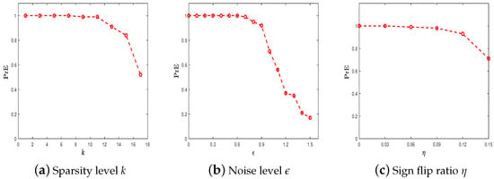
Figure 1. The robustness of MCPWP for various k, $ϵ$, $\eta$ under $p=1000, n=500, \mu =0.3$. (a) $k=1:2:20,$$ϵ=0.01, \eta =0.05$; (b) $k=5, ϵ=0:0.1:1, \eta =0.05$; (c) $k=5, \mu =0.3, ϵ=0.01, \eta$ = 0:0.03:0.15.

4.3. Benchmark Methods

In this test, we try to verify the superiority of our method in comparison with other methods with respect to SNR, the exact probability (PrE(%)), and average computational time (CPU time (s)). The benchmark methods consist of BIHT [4], AOP [6], PBAOP [10], LinProj [29,30], PDASC [15], MCP [12], WPDASC [16], and [17]. Although GPSP is an effective method to improve sparsity in synthesis experiments, GPSP needs the two priors of sparsity. And the first four algorithms and MCP require the prior knowledge of sparsity. In addition, the sign flip rate is specified in AOP and PBAOP. Our method, PDASC, and WPDASC do not need priors. The performance is illustrated in Figure 2 and Figure 3 through the three indexes SNR, PrE, and CPU time when the experiments are conducted at various sparsity level settings. Figure 2 shows that MCPWP and WPDASC exhibit superior performance, while GPSP, MCP, and BIHT are more likely to fail as the sparsity increases. In Figure 3a, MCPWP demonstrates a higher exact recovery probability compared to all other methods except for WPDASC. Meanwhile, it is evident that MCPWP requires less CPU time than WPDASC from Figure 3b. These findings highlight that our method MCPWP is an optimal choice in terms of both performance metrics here. Then, the performance of different methods on the various noise levels with others’ fixed is depicted in Figure 4 and Figure 5. As is plotted, MCPWP generally exhibits a higher SNR than other methods across most scenarios. Notably, for the three noise levels, MCPWP demonstrates the highest SNR, which reveals the robustness of the proposed method. When the sign flip rate becomes larger, our method has a higher SNR and less CPU time, as illustrated in Figure 6 and Figure 7. In addition, with high noise $ϵ$ and a high sign flip rate $\eta$, MCPWP has a higher SNR than the benchmark methods. Additionally, as the sparsity k increases, MCPWP surpasses the other approaches in CPU time except for LinProj (due to its lower computational time as a convex approach). Thus, the above experiments demonstrate that MCPWP is robust against noise, sign flips, and sparsity level, and also outperforms other methods. More higher-dimensional experiments are reported in Table 2. By comparison with other methods, our model is superior.

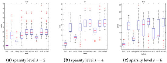
Figure 2. The SNR for different methods with different sparsities. $p=1000,n=500,k$ = 2:2:6, $\mu =0.1,ϵ=0.05,\eta =0.01$.

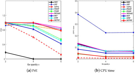
Figure 3. The exact probability and CPU time for different methods with different sparsities. $p=1000,n=500,k$ = 2:2:6, $\mu =0.1,ϵ=0.05,\eta =0.01$.

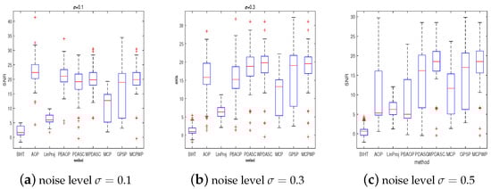
Figure 4. The SNR for different methods with different sparsities. $p=1000,n=500,k=5,$$\mu =0.1,ϵ=0.1:0.2:0.05,\eta =0.01$.

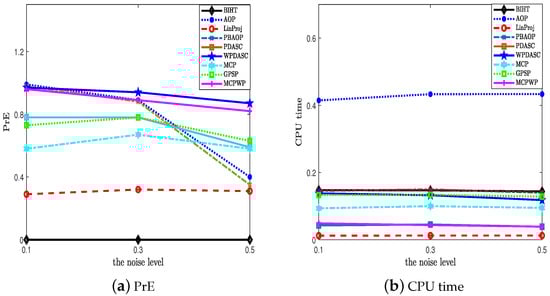
Figure 5. The exact probability and CPU time for different methods with different sparsities. $p=1000,n=500,k=5,\mu =0.1,ϵ=0.1:0.2:0.5,\eta =0.01$.

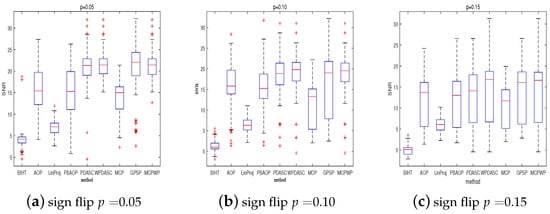
Figure 6. The SNR for different methods with different sparsities. $p=1000,n=500,k=5,$$\mu =0.1,ϵ=0.05,\eta$ = 0.05:0.05:0.15.

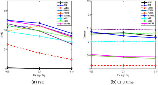
Figure 7. The exact probability and CPU time for different methods on the different sparsity. $p=1000,n=500,k=5,\mu =0.1,ϵ=0.05,\eta$ = 0.05:0.05:0.15.

Table 2. Comparison of many methods under higher-dimension situations.

	(a) $p=\mathrm{10,000},n=2000,k=30$			(b) $p=\mathrm{10,000},n=2000,k=30$			(c) $p=\mathrm{30,000},n=7000,k=20$
	$\mu =0.3,ϵ=0.3,\eta =0.05$			$\mu =0.3,ϵ=0.5,\eta =0.1$			$\mu =0.3,ϵ=0.3,\eta =0.1$
Method	Time (s)	${\ell }_2$-error	PrE (%)	Time (s)	${\ell }_2$-error	PrE (%)	Time (s)	${\ell }_2$-error	PrE (%)
BIHT	4.28	$5.55\times {10}^{-1}$	84	3.82	$7.12\times {10}^{-1}$	0	$8.98\times {10}^{-2}$	$7.06\times {10}^{-1}$	0
AOP	$1.10\times {10}^1$	$1.75\times {10}^{-1}$	100	9.25	$3.19\times {10}^{-1}$	0	$1.10\times {10}^{-1}$	$1.95\times {10}^{-1}$	90
LinProj	$2.16\times {10}^{-1}$	$4.96\times {10}^{-1}$	61	$1.65\times {10}^{-1}$	$5.12\times {10}^{-1}$	0	$4.00\times {10}^{-4}$	$3.59\times {10}^{-1}$	90
PBAOP	4.21	$3.15\times {10}^{-1}$	100	3.68	$2.98\times {10}^{-1}$	0	$3.68\times {10}^{-2}$	$1.68\times {10}^{-1}$	90
PDASC	1.17	$1.19\times {10}^{-1}$	97	$8.85\times {10}^{-1}$	$3.37\times {10}^{-1}$	0	$1.05\times {10}^{-2}$	$6.28\times {10}^{-2}$	100
GPSP	$3.11\times {10}^1$	$2.56\times {10}^{-1}$	89	$6.81\times {10}^2$	1.10	0	6.17	$6.28\times {10}^2$	100
MCP	$8.02\times {10}^{-1}$	$3.24\times {10}^{-1}$	89	$6.34\times {10}^{-1}$	$4.22\times {10}^{-1}$	0	$1.19\times {10}^{-1}$	$6.28\times {10}^{-2}$	100
WPDASC	1.80	$1.19\times {10}^{-1}$	100	1.41	$4.22\times {10}^{-1}$	100	$3.36\times {10}^{-1}$	$6.28\times {10}^{-2}$	100
MCPWP	$6.43\times {10}^{-1}$	$1.58\times {10}^{-1}$	100	$5.89\times {10}^{-1}$	$1.44\times {10}^{-1}$	100	$5.10\times {10}^{-3}$	$6.28\times {10}^{-2}$	100
	(a) $p=\mathrm{25,000},n=5000,k=20$			(b) $p=\mathrm{25,000},n=5000,k=20$			(c) $p=\mathrm{30,000},n=7000,k=20$
	$\mu =0.3,ϵ=0.3,\eta =0.01$			$\mu =0.3,ϵ=0.5,\eta =0.1$			$\mu =0.3,ϵ=0.5,\eta =0.1$
Method	Time (s)	${\ell }_2$-error	PrE (%)	Time (s)	${\ell }_2$-error	PrE (%)	Time (s)	${\ell }_2$-error	PrE (%)
BIHT	$2.37\times {10}^1$	$2.20\times {10}^{-1}$	70	$2.16\times {10}^1$	$6.80\times {10}^{-1}$	0	$3.65\times {10}^2$	$7.91\times {10}^{-1}$	0
AOP	$5.83\times {10}^1$	$1.62\times {10}^{-1}$	80	$5.25\times {10}^1$	$1.91\times {10}^{-1}$	90	$1.09\times {10}^2$	$2.35\times {10}^{-1}$	70
LinProj	$3.36\times {10}^{-1}$	$3.89\times {10}^{-1}$	90	$3.11\times {10}^1$	$3.89\times {10}^{-1}$	100	4.00	$3.61\times {10}^{-1}$	100
PBAOP	$2.18\times {10}^1$	$3.61\times {10}^{-1}$	70	$2.15\times {10}^1$	$2.04\times {10}^{-1}$	100	$3.49\times {10}^1$	$3.59\times {10}^{-1}$	60
PDASC	7.22	$4.93\times {10}^{-2}$	100	$6.16\times {10}^1$	$7.46\times {10}^{-2}$	90	9.80	$7.20\times {10}^{-2}$	100
GPSP	$4.19\times {10}^2$	$4.93\times {10}^2$	100	$4.23\times {10}^2$	$7.46\times {10}^{-2}$	100	$1.44\times {10}^3$	$1.03\times {10}^{-1}$	80
MCP	6.49	$4.93\times {10}^{-2}$	100	5.79	$7.46\times {10}^{-2}$	100	$1.12\times {10}^1$	$7.20\times {10}^{-2}$	100
WPDASC	9.31	$4.93\times {10}^{-2}$	100	6.02	$7.46\times {10}^{-2}$	100	5.44	$7.20\times {10}^{-2}$	100
MCPWP	3.67	$4.93\times {10}^{-2}$	100	3.00	$7.47\times {10}^{-2}$	100	5.20	$7.20\times {10}^{-2}$	100

4.4. Numerical Comparisons on 1-D Real Data

In this section, we aim to decode a 1-dimensional signal from real-world data with $k=15$ under the wavelet basis “Db1” [31]. There is a random Gaussian and an inverse wavelet transform in measurement matrix $A\in {\mathbb{R}}^{n\times p}$ with the noise level $ϵ=0.5$ and sign flip ratio $\eta =0.04$. It should be noted that since GPSP is not suitable for real data, it has been omitted from our analysis. The behaviors of the aforementioned methods are reported in Table 3 and Figure 8. Among three indexes, the peak signal-to-noise ratio (PSNR) is defined as $10log\frac{M^2}{\parallel {\mathbf{x}}_{rec}{-\mathbf{x}\parallel }^2}$, in which M is the absolute value of the maximum in the true vector. In Table 3, as shown in our findings, MCPWP has both higher PSNR values and smaller recovery errors compared to other methods while maintaining a faster CPU time. These results demonstrate the superiority of our decoder.

Table 3. Comparison of methods for 1-D real signal. $p=8000, n=2500, ϵ=0.5, \eta =0.04$.

Method	BIHT	AOP	LinProj	PBAOP	PDASC	WPDASC	MCP	MCPWP
PSNR	28.82	32.65	32.81	30.62	36.44	44.89	35.82	46.32
Err	0.764	0.491	0.482	0.621	0.318	0.120	0.341	0.102
Time (s)	3.299	3.410	0.133	3.493	2.320	2.874	0.358	1.825

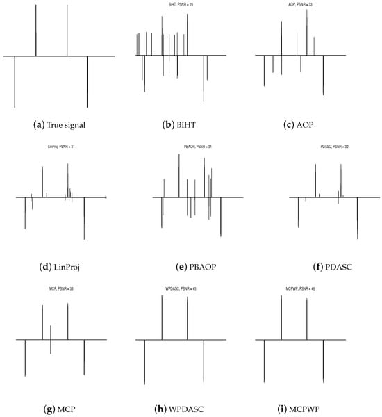
Figure 8. Comparison of different methods under 1-D real signal. $p=8000, n=2500, k=15,$$\mu =0.1, ϵ=0.5, \eta =0.04$.

Finally, we conduct an investigation into the performance of the sparsity-inducing nonconvex regularization function, which contains ${\ell }_q$, MCP, SCAD, and Capped-${\ell }_1$. We utilize the data-driven semi-smooth Newton algorithm equipped with continuity described in [20]. The recovery performance with different regularization functions is presented in Table 4. It is worth noting that the CPU time is very similar across all cases, indicating that the least-squares method with sparsity-inducing nonconvex functions proves to be efficient for 1-bit compressive sensing.

Table 4. Comparison of penalty functions under different situations.

	(a) $p=1000,n=500,k=5$			(b) $p=5000,n=1000,k=15$			(c) $p=\mathrm{20,000},n=5000,k=50$
	$\mu =0.3,ϵ=0.3,\eta =0.05$			$\mu =0.5,ϵ=0.3,\eta =0.05$			$\mu =0,ϵ=0.3,\eta =0.05$
Method	Time (s)	${\ell }_2$-error	PrE (%)	Time (s)	${\ell }_2$-error	PrE (%)	Time (s)	${\ell }_2$-error	PrE (%)
WPDASC	$1.74\times {10}^{-2}$	$8.43\times {10}^{-2}$	100	$2.69\times {10}^{-1}$	$1.44\times {10}^{-1}$	92	5.62	$1.03\times {10}^{-1}$	100
MCPWP	$2.10\times {10}^{-2}$	$8.43\times {10}^{-2}$	100	$1.84\times {10}^{-1}$	$1.48\times {10}^{-1}$	90	4.02	$1.03\times {10}^{-1}$	99
SCAD	$2.30\times {10}^{-2}$	$8.43\times {10}^{-2}$	100	$1.84\times {10}^{-1}$	$1.53\times {10}^{-1}$	88	3.95	$1.03\times {10}^{-1}$	99
Capped-${\ell }_1$	$1.78\times {10}^{-2}$	$8.43\times {10}^{-2}$	100	$1.82\times {10}^{-1}$	$1.45\times {10}^{-1}$	91	1.00	$1.03\times {10}^{-1}$	99

5. Conclusions

In this work, we have analyzed the least-squares regularization approach with MCP and other nonconvex sparsity-inducing functions to reconstruct the signal from 1-bit CS data with added noise and sign flips. We have obtained the competitive complexity of the proposed method, i.e., $m\ge \mathcal{O}\left(\frac{s log n}{{\delta }^2}\right)$ with the accuracy $\delta$ as long as $\eta \ne 1/2$. A data-driven Newton type with an active set and majority-vote selection rule are utilized to implement the unknown signal. Through a lot of numerical simulations, we validate that the proposed model surpasses other state-of-the-art methods.

References

- Boufounos, P.T.; Baraniuk, R.G. 1-bit compressive sensing. In Proceedings of the 2008 42nd Annual Conference on Information Sciences and Systems, Princeton, NJ, USA, 19–21 March 2008; IEEE: Piscataway, NJ, USA, 2008; pp. 16–21. [Google Scholar]
- Fan, X.; Wang, Y.; Huo, Y.; Tian, Z. 1-bit compressive sensing for efficient federated learning over the air. IEEE Trans. Wirel. Commun. 2022, 22, 2139–2155. [Google Scholar] [CrossRef]
- Qing, C.; Ye, Q.; Cai, B.; Liu, W.; Wang, J. Deep learning for 1-bit compressed sensing-based superimposed CSI feedback. PLoS ONE 2022, 17, e0265109. [Google Scholar] [CrossRef]
- Laurent, J.; Jason N., L.; Petros T., B.; Richard G., B. Robust 1-bit compressive sensing via binary stable embeddings of sparse vectors. IEEE Trans. Inf. Theory 2013, 59, 2082–2102. [Google Scholar]
- Matsumoto, N.; Mazumdar, A. Robust 1-bit Compressed Sensing with Iterative Hard Thresholding. In Proceedings of the 2024 Annual ACM-SIAM Symposium on Discrete Algorithms. Society for Industrial and Applied Mathematics, Alexandria, VA, USA, 7–10 January 2024; pp. 2941–2979. [Google Scholar]
- Yan, M.; Yang, Y.; Osher, S. Robust 1-bit compressive sensing using adaptive outlier pursuit. IEEE Trans. Signal Process. 2012, 60, 3868–3875. [Google Scholar] [CrossRef]
- Plan, Y.; Vershynin, R. Robust 1-bit compressed sensing and sparse logistic regression: A convex programming approach. IEEE Trans. Inf. Theory 2012, 59, 482–494. [Google Scholar] [CrossRef]
- Zhang, L.; Yi, J.; Jin, R. Efficient algorithms for robust one-bit compressive sensing. In Proceedings of the International Conference on Machine Learning, Beijing, China, 21–26 June 2014; pp. 820–828. [Google Scholar]
- Dai, D.Q.; Shen, L.; Xu, Y.; Zhang, N. Noisy 1-bit compressive sensing: Models and algorithms. Appl. Comput. Harmon. Anal. 2016, 40, 1–32. [Google Scholar] [CrossRef]
- Huang, X.; Shi, L.; Yan, M.; Suykens, J.A. Pinball loss minimization for one-bit compressive sensing: Convex models and algorithms. Neurocomputing 2018, 314, 275–283. [Google Scholar] [CrossRef]
- Zhu, R.; Gu, Q. Towards a lower sample complexity for robust one-bit compressed sensing. In Proceedings of the International Conference on Machine Learning, Lille, France, 7–9 July 2015; pp. 739–747. [Google Scholar]
- Huang, X.; Yan, M. Nonconvex penalties with analytical solutions for one-bit compressive sensing. Signal Process. 2018, 144, 341–351. [Google Scholar] [CrossRef]
- Xiao, P.; Liao, B.; Li, J. One-bit compressive sensing via Schur-concave function minimization. IEEE Trans. Signal Process. 2019, 67, 4139–4151. [Google Scholar] [CrossRef]
- Plan, Y.; Vershynin, R. The generalized lasso with non-linear observations. IEEE Trans. Inf. Theory 2016, 62, 1528–1537. [Google Scholar] [CrossRef]
- Huang, J.; Jiao, Y.; Lu, X.; Zhu, L. Robust Decoding from 1-Bit Compressive Sampling with Ordinary and Regularized Least Squares. SIAM J. Sci. Comput. 2018, 40, A2062–A2086. [Google Scholar] [CrossRef]
- Fan, Q.; Jia, C.; Liu, J.; Luo, Y. Robust recovery in 1-bit compressive sensing via Lq-constrained least squares. Signal Process. 2021, 179, 107822. [Google Scholar] [CrossRef]
- Zhou, S.; Luo, Z.; Xiu, N.; Li, G.Y. Computing One-bit Compressive Sensing via Double-Sparsity Constrained Optimization. IEEE Trans. Signal Process. 2013, 61, 5777–5788. [Google Scholar] [CrossRef]
- Hou, J.; Liu, X. 1-bit compressed sensing via an l1-tv regularization method. IEEE Access 2022, 10, 116473–116484. [Google Scholar] [CrossRef]
- Zhong, Y.; Xu, C.; Zhang, B.; Hou, J.; Wang, J. One-bit compressed sensing via total variation minimization method. Signal Process. 2023, 207, 108939. [Google Scholar] [CrossRef]
- Huang, J.; Jiao, Y.; Jin, B.; Liu, J.; Lu, X.; Yang, C. A unified primal dual active set algorithm for nonconvex sparse recovery. Statist. Sci. 2021, 36, 215–238. [Google Scholar] [CrossRef]
- Shen, L.; Suter, B.W.; Tripp, E.E. Structured sparsity promoting functions. J. Optim. Theory Appl. 2019, 183, 386–421. [Google Scholar] [CrossRef]
- Plan, Y.; Vershynin, R. One-Bit Compressed Sensing by Linear Programming. Commun. Pure Appl. Math. 2013, 66, 1275–1297. [Google Scholar] [CrossRef]
- Hintermüller, M.; Ito, K.; Kunisch, K. The primal-dual active set strategy as a semismooth Newton method. SIAM J. Optim. 2002, 13, 865–888. [Google Scholar] [CrossRef]
- Zhang, C.H. Nearly unbiased variable selection under minimax concave penalty. Ann. Stat. 2010, 38, 894–942. [Google Scholar] [CrossRef]
- Zhang, C.H.; Zhang, T. A general theory of concave regularization for high-dimensional sparse estimation problems. Stat. Sci. 2012, 27, 576–593. [Google Scholar] [CrossRef]
- Ye, Y.; Zhang, C.H. Rate minimaxity of the Lasso and Dantzig selector for the ℓq loss in ℓr balls. J. Mach. Learn. Res. 2010, 11, 3519–3540. [Google Scholar]
- Gopi, S.; Netrapalli, P.; Jain, P.; Nori, A. One-bit compressed sensing: Provable support and vector recovery. In Proceedings of the International Conference on Machine Learning, Atlanta, GA, USA, 17–19 June 2013; pp. 154–162. [Google Scholar]
- Kim, Y.; Kwon, S.; Choi, H. Consistent model selection criteria on high dimensions. J. Mach. Learn. Res. 2012, 13, 1037–1057. [Google Scholar]
- Plan, Y.; Vershynin, R.; Yudovina, E. High-dimensional estimation with geometric constraints. Inf. Inference A J. IMA 2016, 6, 1–40. [Google Scholar]
- Vershynin, R. Estimation in high dimensions: A geometric perspective. In Sampling Theory, a Renaissance; Springer: Berlin/Heidelberg, Germany, 2015; pp. 3–66. [Google Scholar]
- Mallat, S. A Wavelet Tour of Signal Processing: The Sparce Way, 3rd ed.; AP Professional: London, UK, 2009. [Google Scholar]
Disclaimer/Publisher’s Note: The statements, opinions and data contained in all publications are solely those of the individual author(s) and contributor(s) and not of MDPI and/or the editor(s). MDPI and/or the editor(s) disclaim responsibility for any injury to people or property resulting from any ideas, methods, instructions or products referred to in the content. |
© 2024 by the authors. Licensee MDPI, Basel, Switzerland. This article is an open access article distributed under the terms and conditions of the Creative Commons Attribution (CC BY) license (https://creativecommons.org/licenses/by/4.0/).