Command-Filtered Nussbaum Design for Nonlinear Systems with Unknown Control Direction and Input Constraints

Abstract

This paper studies the problem of adaptive fuzzy control based on command filtering for a class of nonlinear systems characterized by an input dead zone, input saturation, and unknown control direction. First, this paper proposes a novel equivalent transformation technique that simplifies the design complexity of multiple input constraints by converting the input dead zone and saturation nonlinearities into a unified functional form. Subsequently, a fuzzy logic system is utilized to handle the unknown nonlinear functions, and the command-filtering method is employed to address the issue of complexity explosion, while the Nussbaum function is utilized to resolve the challenge of an unknown control direction. Based on Lyapunov stability, it is proven that the tracking error converges to a small neighborhood around the origin, and all closed-loop signals are bounded. Finally, a numerical simulation result and an actual simulation result of a pendulum are presented to verify the feasibility and effectiveness of the proposed control strategy.

1. Introduction

It is widely acknowledged that stability analysis and controller design for nonlinear systems have been subjects of ongoing research and interest for several decades [1,2,3]. This technology is often applied to robots [4], quadcopter UAVs [5], noise data classification [6], aerospace systems [7], etc. Recently, the combination of backstepping methodology with adaptive control techniques to address nonlinear systems has undergone significant development and practical application. In earlier studies, nonlinear terms of the system were often assumed to be known a priori or linearly parameterizable. However, for many practical systems, this assumption is considered unrealistic. To solve this problem, neural networks (NNs) and fuzzy logic systems (FLS) have been used to approximate unknown system dynamics [8,9]. For example, [10] introduced an adaptive fuzzy controller grounded in sliding mode control theory. In [11,12,13], the authors introduced several intelligent control methodologies for nonlinear systems featuring pure feedback structures by amalgamating neural networks or fuzzy logic systems with adaptive backstepping approaches.

However, the most common drawback of backstepping techniques is the complexity explosion caused by repeatedly differentiating the virtual controller. To address this issue, Ref. [14] proposed a dynamic surface control (DSC) scheme, which incorporated a first-order filter dynamic surface at each stage of the backstepping control design process, thereby obviating the need for calculating the derivatives of the virtual controller. Dynamic filtering technology was introduced by [15] to investigate event-triggered tracking control of a category of uncertain nonlinear systems. However, DSC technology failed to account for the error introduced by the filter, consequently diminishing the control performance of the system. Refs. [16,17,18,19] applied command-filtering technology to nonlinear systems under different constraints, which not only solved the problem of complexity explosion in the backstepping design process, but also established an error compensation system to make up for the shortcomings of DSC technology.

Despite the success of command-filter adaptive control in nonlinear systems, the presence of various constraints in practical engineering contexts, such as input dead zones, input saturation, unknown control direction, etc., can influence the system’s stability. To solve the dead-zone problem, some related results are provided in [20,21,22]. Ref. [20] proposed an adaptive dead-zone inverse technology. Ref. [21] developed a corresponding disturbance observer for estimation based on the unknown approximation error and the impact of unknown dead zones and external disturbances. In [22], the system was converted into n-step predictors, and an adaptive compensation term was introduced to overcome the asymmetric dead zone existing in the system. Apart from the presence of dead zone input, the presence of input saturation can also cause performance degradation of nonlinear systems and signal delay or loss. The study of input saturated systems has also been an important topic in recent years [23,24].

On the other hand, when researching adaptive control of nonlinear systems, it is often necessary to know the control direction representing the direction of motion in advance [25,26]. However, the direction of controlling gain is mostly unknown in practical applications. The Nussbaum gain method is an effective tool for processing unknown signals. Characterized by its values and integral oscillating infinitely between positive and negative, the Nussbaum function allows the control system to adjust its strategy automatically, despite uncertainty about the sign of the control gain, ensuring that the system can stably achieve the desired state. Building upon this technology, numerous control strategies have been formulated [27,28,29,30]. Ref. [27] introduced the Nussbaum function to compensate for the impact of the unknown direction problem and designed an adaptive tracking controller based on a command filter. For systems featuring multiple unknown high-frequency gains, Ref. [28] introduced a novel command-filtered Nussbaum design. A novel Nussbaum function was devised by [29] to address the tracking problem encountered within a category ofstochastic strict feedback nonlinear systems. By using an improved Nussbaum function, [30] extended previous research results to cover a broader range of nonlinear systems, characterized by unknown variations in both the sign and magnitude of the control gain over time. However, to the best of our knowledge, there is a scarcity of papers that concurrently address nonlinear systems with input dead zones, input saturation, and uncertain control directions. This scarcity partly motivated the research presented in this paper.

Based on the previous discussion, the main contributions of this article, in contrast to existing research outcomes, can be encapsulated as follows:

• Compared with the nonlinear systems studied in [25,26], where the control direction was known, this paper considers a broader situation in which the control direction is unknown, and it designs adaptive fuzzy control using the Nussbaum function.
• This paper proposes a novel transformation method to eliminate the impact of the input dead zone and saturation on the system, and uses command-filtering technology to solve the problem of complexity explosion in traditional backstepping design.

2. Preliminary Knowledge and Problem Statement

2.1. System Model

Consider the following nonlinear system

$$\left\{\begin{array}{c}{\dot{x}}_i=f_i\left({\overline{x}}_i\right)+{\lambda }_i{g}_i\left({\overline{x}}_i\right)x_{i+1},i=1,\dots ,n-1,\hfill \\ {\dot{x}}_n=f_n\left({\overline{x}}_n\right)+{\lambda }_n{g}_n\left({\overline{x}}_n\right)u,\hfill \\ y=x_1,\hfill \end{array}\right.$$

(1)

where $x={\left[x_1,x_2,\dots x_n\right]}^T\in R^n$ represents the state vector with ${\overline{x}}_i={[x_1,x_2,\dots x_i]}^T\in R^i$, and $y\in R$ denotes the system output; ${\lambda }_i=1$ (or −1) represents an unknown control direction; $g_i\left({\overline{x}}_i\right)$ are bounded continuous functions with $0<{\hslash }_i\le g_i(·)\le {\mathsf{\Theta }}_i$, ${\hslash }_i$ and ${\mathsf{\Theta }}_i$ represent two constants; and $f_i\left({\overline{x}}_i\right)$ signifies the unknown smooth function. The control input $u\in R$ is specified as

$$u\left(t\right)=\left\{\begin{array}{cc}{u}_h,\hfill & v\left(t\right)>u_h,\hfill \\ k_h\left(v\left(t\right)-m_h\right),\hfill & m_h\le v\left(t\right)<u_h,\hfill \\ 0,\hfill & -m_l<v\left(t\right)\le m_h,\hfill \\ k_l\left(v\left(t\right)+m_l\right),\hfill & -u_l<v\left(t\right)\le -m_l,\hfill \\ -u_l,\hfill & v\left(t\right)<-u_l,\hfill \end{array}\right.$$

(2)

where $v\left(t\right)$ is the input of the dead zone; $u_h$ and $u_l$ are positive parameters and represent unknown saturation values; $k_h>0$, $k_l>0$, $m_h>0$, and $m_l>0$ are the unknown zone parameters; and the dead-zone slopes in positive and negative region are same, i.e., $k_h=k_l=k$.

Assumption 1 ([22]).

The dead-zone parameters of $m_h$, $m_l$, and k are bounded. This implies that there are known parameters $m_{h max}$, $m_{h min}$, $m_{l max}$, $m_{l min}$, $k_{max}$, and $k_{min}$, such that $m_h\in \left[m_{h min},m_{h max}\right]$, $m_l\in \left[m_{l min},m_{l max}\right]$, and $k\in \left[k_{min},k_{max}\right]$.

For the development of a robust control scheme, (2) is reformulated as follows:

$$u\left(t\right)=\pi \left(v\left(t\right)\right)v\left(t\right)+\vartheta \left(v\left(t\right)\right).$$

(3)

Based on Assumption 1, one can conclude that $\vartheta \left(v\left(t\right)\right)$ is bounded, while satisfies $\left|\vartheta \left(v\left(t\right)\right)\right|\le L_p$, where $L_p$ represents the upper bound.

Assumption 2 ([25]).

In this article, considering that the input signal v is limited in actual situations, $\pi \left(v\left(t\right)\right)$ satisfies the following inequality

$$0<\Im \le min\left\{\frac{u_h}{v{\left(t\right)}_{max}},k\right\}\le \pi \left(v\left(t\right)\right)\le max\left\{1,k\right\},$$

(4)

2.2. Fuzzy Logic Systems

FLS consists of four primary components: the knowledge base, fuzzifier, fuzzy inference engine, and defuzzifier. The knowledge base houses a comprehensive set of fuzzy if-then rules, which are defined as follows:

$R^l$: IF $x_1$ is $P_1^j$, and $x_2$ is $P_2^j$, and $x_n$ is $P_n^j$, then y is $Q^j$,$j=1,2,\dots ,\wp ,$ where $x={\left[x_1,x_2,\dots ,x_n\right]}^T$, and y are the FLSs input and system output, respectively; $P_m^j$, $Q^j$ denote the fuzzy sets for x and y, respecitvley; an equivalent expression of FLS can be obtained as

$$y\left(x\right)=\frac{{\sum }_{j=1}^{\wp }{\overline{y}}_j{\prod }_{m=1}^n{\mu }_{F_m^j}\left(x_m\right)}{{\sum }_{j=1}^{\wp }\left[{\prod }_{m=1}^n{\mu }_{F_m^j}\left(x_m\right)\right]},$$

(5)

with ${\overline{y}}_j={max}_{y\in R}{\mu }_{Q^j}\left(y\right)$, where ${\mu }_{P_m^j}\left(x_m\right)$ and ${\mu }_{Q^j}\left(y\right)$ are the membership functions. Denote $W={[{\overline{y}}_1,{\overline{y}}_2,\dots ,{\overline{y}}_{\wp }]}^T={[W_1,W_2,\dots ,W_{\wp }]}^T$ and $\psi \left(x\right)={\left[{\psi }_1\left(x\right),{\psi }_2\left(x\right),\dots ,{\psi }_{\wp }\left(x\right)\right]}^T$, the membership functions, which are defined as ${\psi }_j\left(x\right)=\frac{{\prod }_{m=1}^n{\mu }_{F_m^j}\left(x_m\right)}{{\sum }_{j=1}^{\wp }\left[{\prod }_{m=1}^n{\mu }_{F_m^j}\left(x_m\right)\right]}$. Consequently, FLS can be succinctly described as follows

$$y\left(x\right)=W^T\psi \left(x\right).$$

(6)

Lemma 1 ([27]).

The following inequality holds for any smooth function $f\left(x\right)$ defined on the compact set Ω if there is a sufficiently tiny positive scalar ε:

$$\underset{x\in \mathsf{\Omega }}{sup}\left|f\left(x\right)-W^{\mathrm{T}}\psi \left(x\right)\right|\le \epsilon .$$

(7)

Definition 1 ([29]).

The Nussbaum function $N\left(\zeta \right):\mathbb{R}\to \mathbb{R}$ has the properties

$$\begin{array}{cc}& \underset{\ell \to \infty }{lim}sup\frac{1}{\ell }{\int }_0^{\ell }N\left(\zeta \right)d\zeta =+\infty ,\hfill \\ & \underset{\ell \to -\infty }{lim}inf\frac{1}{\ell }{\int }_0^{\ell }N\left(\zeta \right)d\zeta =-\infty .\hfill \end{array}$$

(8)

Lemma 2 ([29]).

Consider $\zeta \left(t\right)$ and $V\left(t\right)\ge 0$ are smooth functions on $[0,t_f)$, and $N\left(\zeta \left(t\right)\right)$ is an even smooth Nussbaum-type function. Suppose

$$V\left(t\right)\le e^{-{{\rm Y}}_{1}t}{\int }_0^t\left(w\left(\overline{x}\left(\tau \right)\right)N\left(\zeta \left(\tau \right)\right)+1\right)\dot{\zeta }\left(\tau \right)e^{{{\rm Y}}_1\tau }d\tau +D,$$

(9)

in which $D>0$ and ${{\rm Y}}_1>0$, and $V\left(t\right)$, $\zeta \left(t\right)$ and ${\int }_0^{t}w\left(\overline{x}\left(\tau \right)\right)N\left(\zeta \left(\tau \right)\right)\dot{\zeta }\left(\tau \right)d\tau$ remain bounded on $[0,t_f)$.

Lemma 3 ([25]).

The command filter is defined as

$$\left\{\begin{array}{c}{\dot{\omega }}_i=\varpi {\omega }_{i,2},\hfill \\ {\dot{\omega }}_{i,2}=-2\phi \varpi {\omega }_{i,2}-\varpi ({\omega }_i-{\alpha }_{i-1}),\hfill \end{array}\right.$$

(10)

where ${\alpha }_{i-1}$ and ${\omega }_i$ represent the input and output of the command filter, respectively, ${\omega }_i\left(0\right)={\alpha }_{i-1}$ and ${\omega }_{i,2}\left(0\right)=0$, $\phi \in (0,1]$, and $\varpi >0$.

Remark 1.

The command-filtering approach is a control strategy that simplifies the design and implementation of complex control systems. By incorporating a filter between the controller and actuator, it smooths the control signals, preventing performance degradation due to overly complex control strategies. This method effectively reduces system complexity and avoids “complexity explosion” caused by high-frequency control updates and excessive regulation.

Assumption 3 ([26]).

The reference signal $x_d$ and its first-order derivative ${\dot{x}}_d$ are continuous and bounded.

3. Controller Design and Stability Analysis

3.1. Controller Design

In this section, an adaptive command-filter controller is designed for the nonlinear system (1) by integrating the Nussbaum function with the back-stepping technique. Coordinate changes are introduced to facilitate controller design:

$$\left\{\begin{array}{c}{e}_1=x_1-y_d,\hfill \\ e_i=x_i-{\omega }_i,i=1,\dots ,n,\hfill \end{array}\right.$$

(11)

where $e_i$ represents the tracking error and ${\omega }_i$ denotes the output of the filter.

Remark 2.

It is noteworthy that the error induced by the command filter exacerbates the system error. To address this drawback, a compensation signal, denoted as β, is introduced to mitigate the adverse effects of the filter error ${\omega }_i-{\alpha }_{i-1}$ on the system.

Design the compensation signal ${\beta }_i$ to eliminate the error caused by the command filter as follows

$$\left\{\begin{array}{c}{\dot{\beta }}_i=-k_i{\beta }_i+g_i{\beta }_{i+1}+g_i\left({\omega }_{i+1}-{\alpha }_i\right),\hfill \\ {\dot{\beta }}_n=-k_n{\beta }_n,\hfill \end{array}\right.$$

(12)

where $k_i$ is a given positive constant and ${\beta }_i\left(0\right)=0$.

Subsequently, the compensated tracking error signals can be expressed as follows

$${\xi }_i=e_i-{\beta }_i,i=1,2,\dots ,n.$$

(13)

Step 1: Taking the derivative of ${\xi }_i$ as

$$\begin{array}{cc}\hfill {\dot{\xi }}_1& ={\dot{e}}_1-{\dot{\beta }}_1={\dot{x}}_1-{\dot{y}}_d-{\dot{\beta }}_1=f_1+{\lambda }_1{g}_1{x}_2-{\dot{y}}_d-{\dot{\beta }}_1.\hfill \end{array}$$

(14)

The Lyapunov function is chosen as

$$V_1=\frac{1}{2}{\xi }_1^2+\frac{1}{2{\mathsf{\Gamma }}_1}{\tilde{\theta }}_1^2,$$

(15)

where ${\mathsf{\Gamma }}_1$ represents the positive parameter to be constructed, and in order to solve the parameter estimation problem, the parameter estimation error is ${\tilde{\theta }}_1={\theta }_1-{\hat{\theta }}_1$, and the constant is defined as ${\theta }_i={∥W_i∥}^2$.

Based on (11), (13), (14) and (15) the time derivative of $V_1$ is shown as

$$\begin{array}{cc}\hfill {\dot{V}}_1& ={\xi }_1{\dot{\xi }}_1-\frac{1}{{\mathsf{\Gamma }}_1}{\tilde{\theta }}_1{\dot{\hat{\theta }}}_1\hfill \\ \hfill & ={\xi }_1\left(f_1+{\lambda }_1{g}_1\left({\omega }_2+{\xi }_2+{\beta }_2\right)-{\dot{y}}_d-{\dot{\beta }}_1\right)-\frac{1}{{\mathsf{\Gamma }}_1}{\tilde{\theta }}_1{\dot{\hat{\theta }}}_1\hfill \\ \hfill & ={\xi }_1{f}_1+{\lambda }_1{g}_1{\xi }_1{\omega }_2+{\lambda }_1{g}_1{\xi }_1{\xi }_2+{\lambda }_1{g}_1{\xi }_1{\beta }_2-{\xi }_1{\dot{y}}_d-{\xi }_1{\dot{\beta }}_1-\frac{1}{{\mathsf{\Gamma }}_1}{\tilde{\theta }}_1{\dot{\hat{\theta }}}_1.\hfill \end{array}$$

(16)

As function $f_1\left(x\right)$ is unknown, the direct design of the virtual control signal ${\alpha }_1$ is not feasible. Thus, according to Lemma 1, for any given number ${\epsilon }_1>0$, there are

$$f_1\left(B_1\right)=W_1^T{\psi }_1+{\delta }_1\left(B_1\right),\parallel {\delta }_1\left(B_1\right)\parallel <{\epsilon }_1,$$

in which $\parallel {\delta }_1\left(B_1\right)\parallel$ denotes the estimation error.

By applying Young’s inequality, the following formula can be derived

$${\xi }_1{f}_1\le \frac{{\xi }_1^2{\theta }_1{S}_1^T{S}_1}{2a_1^2}+\frac{1}{2}{a}_1^2+\frac{1}{2}{\xi }_1^2+\frac{1}{2}{\epsilon }_1^2,$$

(17)

where $a_1$ is a given positive scalar.

Consider a compensating signal ${\dot{\beta }}_1$ as

$${\dot{\beta }}_1=-k_1{\beta }_1+g_1{\beta }_2+g_1\left({\omega }_2-{\alpha }_1\right).$$

(18)

Next, after combining Formulas (16)–(18), it can be easily obtained that

$$\begin{array}{cc}\hfill {\dot{V}}_1\le & \frac{{\xi }_1^2{\theta }_1{S}_1^T{S}_1}{2a_1^2}+\frac{1}{2}{a}_1^2+\frac{1}{2}{\xi }_1^2+\frac{1}{2}{\epsilon }_1^2+{\lambda }_1{g}_1{\xi }_1{\omega }_2+{\lambda }_1{g}_1{\xi }_1{\xi }_2+{\lambda }_1{g}_1{\xi }_1{\beta }_2\hfill \\ \hfill & +k_1{\xi }_1{\beta }_1-g_1{\xi }_1{\beta }_2-g_1{\xi }_1{\omega }_2+g_1{\xi }_1{\alpha }_1-\frac{1}{{\mathsf{\Gamma }}_1}{\tilde{\theta }}_1{\dot{\hat{\theta }}}_1-{\xi }_1{\dot{y}}_d\hfill & \\ \hfill \le & \frac{{\xi }_1^2{\theta }_1{S}_1^T{S}_1}{2a_1^2}+\frac{1}{2}{a}_1^2+\frac{1}{2}{\xi }_1^2+\frac{1}{2}{\epsilon }_1^2+{\lambda }_1{g}_1{\xi }_1{\xi }_2+k_1{\xi }_1{\beta }_1+g_1{\xi }_1{\alpha }_1-\frac{1}{{\mathsf{\Gamma }}_1}{\tilde{\theta }}_1{\dot{\hat{\theta }}}_1\hfill \\ \hfill & +\left(\begin{array}{c}{\lambda }_1-1\end{array}\right)g_1{\xi }_1\left(\begin{array}{c}{\beta }_2+{\omega }_2\end{array}\right)-{\xi }_1{\dot{y}}_d.\hfill \end{array}$$

(19)

In this article, ${\lambda }_1=1(or-1)$ represents the unknown control direction. Applying Young’s inequality, one can obtain

$$\begin{array}{cc}\hfill \left({\lambda }_1-1\right)g_1{\xi }_1\left({\beta }_2+{\omega }_2\right)=\left({\lambda }_1-1\right)g_1{\xi }_1\left(x_2-{\xi }_2\right)=0\le 2g_1^2{\xi }_1^2+x_2^2+{\xi }_2^2,& {\lambda }_1=1,\hfill \\ \hfill \left({\lambda }_1-1\right)g_1{\xi }_1\left({\beta }_2+{\omega }_2\right)=\left({\lambda }_1-1\right)g_1{\xi }_1\left(x_2-{\xi }_2\right)\le 2g_1^2{\xi }_1^2+x_2^2+{\xi }_2^2,& {\lambda }_1=-1,\hfill \\ \hfill {\lambda }_1{g}_1{\xi }_1{\xi }_2\le \frac{1}{2}{g}_1^2{\xi }_1^2+\frac{1}{2}{\xi }_2^2,& {\lambda }_1=1(or-1).\hfill \end{array}$$

(20)

Substituting (20) into (19) produces

$$\begin{array}{cc}\hfill {\dot{V}}_1\le & \frac{{\xi }_1^2{\theta }_1{\psi }_1^T{\psi }_1}{2a_1^2}+\frac{1}{2}{a}_1^2+\frac{1}{2}{\xi }_1^2+\frac{1}{2}{\epsilon }_1^2+\frac{5}{2}{g}_1^2{\xi }_1^2+\frac{3}{2}{\xi }_2^2\hfill \\ \hfill & +k_1{\xi }_1{\beta }_1+g_1{\xi }_1{\alpha }_1-\frac{1}{{\mathsf{\Gamma }}_1}{\tilde{\theta }}_1{\dot{\hat{\theta }}}_1+x_2^2-{\xi }_1{\dot{y}}_d.\hfill \end{array}$$

(21)

Next, the virtual control signal ${\alpha }_1$ and the Nussbaum-type gain ${\zeta }_1$ are developed as follows

$$\left\{\begin{array}{c}{\alpha }_1=N\left({\zeta }_1\right)\left(\frac{{\xi }_1{\hat{\theta }}_1{S}_1^T{S}_1}{2a_1^2}+k_1{e}_1+\frac{1}{2}{\xi }_1+\frac{5}{2}{g}_1^2{\xi }_1-{\dot{y}}_d\right),\hfill \\ {\dot{\zeta }}_1={\xi }_1\left(\frac{{\xi }_1{\hat{\theta }}_1{S}_1^T{S}_1}{2a_1^2}+k_1{e}_1+\frac{1}{2}{\xi }_1+\frac{5}{2}{g}_1^2{\xi }_1-{\dot{y}}_d\right).\hfill \end{array}\right.$$

(22)

By amalgamating the aforementioned equation, (21) can be reformulated as

$$\begin{array}{cc}\hfill {\dot{V}}_1& \le \frac{{\xi }_1^2{\theta }_1{\psi }_1^T{\psi }_1}{2a_1^2}+\frac{1}{2}{a}_1^2+\frac{1}{2}{\xi }_1^2+\frac{1}{2}{\epsilon }_1^2+\frac{5}{2}{g}_1^2{\xi }_1^2+\frac{3}{2}{\xi }_2^2+k_1{\xi }_1{\beta }_1+g_1{\xi }_1{\alpha }_1-\frac{1}{{\mathsf{\Gamma }}_1}{\tilde{\theta }}_1{\dot{\hat{\theta }}}_1+x_2^2-{\xi }_1{\dot{y}}_d\hfill \\ \hfill & \le -k_1{\xi }_1^2+g_{1}N\left({\zeta }_1\right){\dot{\zeta }}_1+{\dot{\zeta }}_1+\frac{{\tilde{\theta }}_1}{{\mathsf{\Gamma }}_1}\left(\frac{{\mathsf{\Gamma }}_1{\xi }_1^2{\psi }_1^T{\psi }_1}{2a_1^2}-{\dot{\hat{\theta }}}_1\right)+\frac{1}{2}{a}_1^2+\frac{1}{2}{\epsilon }_1^2+\frac{3}{2}{\xi }_2^2+x_2^2.\hfill \end{array}$$

(23)

Next, the adaptive law ${\dot{\hat{\theta }}}_1$ is designed as ${\dot{\hat{\theta }}}_1=\frac{{\mathsf{\Gamma }}_1{\xi }_1^2{\psi }_1^T{\psi }_1}{2a_1^2}-{\sigma }_1{\hat{\theta }}_1$, and with the help of Young’s inequality $\frac{{\sigma }_1{\tilde{\theta }}_1{\hat{\theta }}_1}{{\mathsf{\Gamma }}_1}\le \frac{{\sigma }_1{\theta }_1^2}{2{\mathsf{\Gamma }}_1}-\frac{{\sigma }_1{\tilde{\theta }}_1^2}{2{\mathsf{\Gamma }}_1}$, one obtain

$${\dot{V}}_1\le -k_1{\xi }_1^2+g_{1}N\left({\zeta }_1\right){\dot{\zeta }}_1+{\dot{\zeta }}_1-\frac{{\sigma }_1{\tilde{\theta }}_1^2}{2{\mathsf{\Gamma }}_1}+N_1,$$

(24)

where $N_1=\frac{1}{2}{a}_1^2+\frac{1}{2}{\epsilon }_1^2+\frac{3}{2}{\xi }_2^2+x_2^2+\frac{{\sigma }_1{\theta }_1^2}{2{\mathsf{\Gamma }}_1}$.

• Step i: $(2\le i\le n-1)$: According to the differential rules, the following expression is derived

  $$\begin{array}{cc}\hfill {\dot{\xi }}_i& ={\dot{e}}_i-{\dot{\beta }}_i={\dot{x}}_i-{\dot{\omega }}_i-{\dot{\beta }}_i=f_i+{\lambda }_i{g}_i{x}_{i+1}-{\dot{\omega }}_i-{\dot{\beta }}_i.\hfill \end{array}$$

  (25)

Choose a Lyapunov function candidate function, as follows

$$V_i=V_{i-1}+\frac{1}{2}{\xi }_i^2+\frac{1}{2{\mathsf{\Gamma }}_i}{\tilde{\theta }}_i^2.$$

(26)

where ${\tilde{\theta }}_i={\theta }_i-{\hat{\theta }}_i$.

By differentiating $V_i$, the following formula holds

$$\begin{array}{cc}\hfill {\dot{V}}_i& ={\dot{V}}_{i-1}+{\xi }_i{\dot{\xi }}_i-\frac{1}{{\mathsf{\Gamma }}_i}{\tilde{\theta }}_i{\dot{\hat{\theta }}}_i\hfill \\ \hfill & ={\dot{V}}_{i-1}+{\xi }_i\left(f_i+{\lambda }_i{g}_i\left({\omega }_{i+1}+{\xi }_{i+1}+{\beta }_{i+1}\right)-{\dot{\omega }}_i-{\dot{\beta }}_i\right)-\frac{1}{{\mathsf{\Gamma }}_i}{\tilde{\theta }}_i{\dot{\hat{\theta }}}_i\hfill \\ \hfill & ={\dot{V}}_{i-1}+{\xi }_i{f}_i+{\lambda }_i{g}_i{\xi }_i{\omega }_{i+1}+{\lambda }_i{g}_i{\xi }_i{\xi }_{i+1}+{\lambda }_i{g}_i{\xi }_i{\beta }_{i+1}-{\xi }_i{\dot{\omega }}_i-{\xi }_i{\dot{\beta }}_i-\frac{1}{{\mathsf{\Gamma }}_i}{\tilde{\theta }}_i{\dot{\hat{\theta }}}_i.\hfill \end{array}$$

(27)

According to Lemma 1 again, for any given number ${\epsilon }_i>0$, there are

$$f_i\left(B_i\right)=W_i^T{\psi }_i+{\delta }_i\left(B_i\right),\parallel {\delta }_i\left(B_i\right)\parallel <{\epsilon }_i,$$

in which $\parallel {\delta }_i\left(B_i\right)\parallel$ denotes the estimation error.

By applying Young’s inequality again, the following formula can be derived

$${\xi }_i{f}_i\le \frac{{\xi }_i^2{\theta }_i{\psi }_i^T{\psi }_i}{2a_i^2}+\frac{1}{2}{a}_i^2+\frac{1}{2}{\xi }_i^2+\frac{1}{2}{\epsilon }_i^2,$$

(28)

where $a_i$ is a given positive scalar.

The compensation signal ${\dot{\beta }}_i$ is designed to be

$${\dot{\beta }}_i=-k_i{\beta }_i+g_i{\beta }_{i+1}+g_i\left({\omega }_{i+1}-{\alpha }_i\right).$$

(29)

Incorporating Equations (28) and (29) into (27), one can obtain

$$\begin{array}{cc}\hfill {\dot{V}}_i\le & {\dot{V}}_{i-1}+\frac{{\xi }_i^2{\theta }_i{\psi }_i^T{\psi }_i}{2a_i^2}+\frac{1}{2}{a}_i^2+\frac{1}{2}{\xi }_i^2+\frac{1}{2}{\epsilon }_i^2+{\lambda }_i{g}_i{\xi }_i{\xi }_{i+1}+k_i{\xi }_i{\beta }_i+g_i{\xi }_i{\alpha }_i-\frac{1}{{\mathsf{\Gamma }}_i}{\tilde{\theta }}_i{\dot{\hat{\theta }}}_i\hfill \\ \hfill & +\left[\begin{array}{c}{\lambda }_i{g}_i{\xi }_i{\omega }_{i+1}+{\lambda }_i{g}_i{\xi }_i{\beta }_{i+1}-g_i{\xi }_i{\beta }_{i+1}-g_i{\xi }_i{\omega }_{i+1}\end{array}\right]-{\xi }_i{\dot{\omega }}_i\hfill \\ \hfill \le & {\dot{V}}_{i-1}+\frac{{\xi }_i^2{\theta }_i{\psi }_i^T{\psi }_i}{2a_i^2}+\frac{1}{2}{a}_i^2+\frac{1}{2}{\xi }_i^2+\frac{1}{2}{\epsilon }_i^2+{\lambda }_i{g}_i{\xi }_i{\xi }_{i+1}+k_i{\xi }_i{\beta }_i+g_i{\xi }_i{\alpha }_i-\frac{1}{{\mathsf{\Gamma }}_i}{\tilde{\theta }}_i{\dot{\hat{\theta }}}_i\hfill \\ \hfill & +\left(\begin{array}{c}{\lambda }_i-1\end{array}\right)g_i{\xi }_i\left(\begin{array}{c}{\beta }_{i+1}+{\omega }_{i+1}\end{array}\right)-{\xi }_i{\dot{\omega }}_i.\hfill \end{array}$$

(30)

Similar to (20), one can obtain

$$\begin{array}{cc}\hfill {\lambda }_i{g}_i{\xi }_i{\xi }_{i+1}& \le \frac{1}{2}{g}_i^2{\xi }_i^2+\frac{1}{2}{\xi }_{i+1}^2,\hfill \\ \hfill \left({\lambda }_i-1\right)g_i{\xi }_i\left({\beta }_{i+1}+{\omega }_{i+1}\right)& \le 2g_i^2{\xi }_i^2+x_{i+1}^2+{\xi }_{i+1}^2.\hfill \end{array}$$

(31)

Then, (30) is rewritten as

$$\begin{array}{cc}\hfill {\dot{V}}_1\le & {\dot{V}}_{i-1}+\frac{{\xi }_i^2{\theta }_i{\psi }_i^T{\psi }_i}{2a_i^2}+\frac{1}{2}{a}_i^2+\frac{1}{2}{\xi }_i^2+\frac{1}{2}{\epsilon }_i^2+\frac{5}{2}{g}_i^2{\xi }_i^2+\frac{3}{2}{\xi }_{i+1}^2\hfill \\ \hfill & +k_i{\xi }_i{\beta }_i+g_i{\xi }_i{\alpha }_i-\frac{1}{{\mathsf{\Gamma }}_i}{\tilde{\theta }}_i{\dot{\hat{\theta }}}_i+x_{i+1}^2-{\xi }_i{\dot{\omega }}_i.\hfill \end{array}$$

(32)

The virtual control signal ${\alpha }_1$ and the Nussbaum-type gain ${\zeta }_1$ are designed as

$$\left\{\begin{array}{c}{\alpha }_i=N\left({\zeta }_i\right)\left(\frac{{\xi }_i{\hat{\theta }}_i{\psi }_i^T{\psi }_i}{2a_i^2}+k_i{e}_i+\frac{1}{2}{\xi }_i+\frac{5}{2}{g}_i^2{\xi }_i-{\dot{\omega }}_i\right),\hfill \\ {\dot{\zeta }}_i={\xi }_i\left(\frac{{\xi }_i{\hat{\theta }}_i{\psi }_i^T{\psi }_i}{2a_i^2}+k_i{e}_i+\frac{1}{2}{\xi }_i+\frac{5}{2}{g}_i^2{\xi }_i-{\dot{\omega }}_i\right).\hfill \end{array}\right.$$

(33)

Combining the above equation, (32) can be rewritten as

$$\begin{array}{cc}\hfill {\dot{V}}_i& \le {\dot{V}}_{i-1}-k_i{\xi }_i^2+g_{i}N\left({\zeta }_i\right){\dot{\zeta }}_i+{\dot{\zeta }}_i+\frac{{\tilde{\theta }}_i}{{\mathsf{\Gamma }}_i}\left(\frac{{\mathsf{\Gamma }}_i{\xi }_i^2{\psi }_i^T{\psi }_i}{2a_i^2}-{\dot{\hat{\theta }}}_i\right)+\frac{1}{2}{a}_i^2+\frac{1}{2}{\epsilon }_i^2+\frac{3}{2}{\xi }_{i+1}^2+x_{i+1}^2.\hfill \end{array}$$

(34)

Next, the adaptive law ${\dot{\hat{\theta }}}_i$ is designed as ${\dot{\hat{\theta }}}_i=\frac{{\mathsf{\Gamma }}_i{\xi }_i^2{\psi }_i^T{\psi }_i}{2a_i^2}-{\sigma }_i{\hat{\theta }}_i$, and with the help of Young’s inequality $\frac{{\sigma }_i{\tilde{\theta }}_i{\hat{\theta }}_i}{{\mathsf{\Gamma }}_i}\le \frac{{\sigma }_i{\theta }_i^2}{2{\mathsf{\Gamma }}_i}-\frac{{\sigma }_i{\tilde{\theta }}_i^2}{2{\mathsf{\Gamma }}_i}$, one obtain

$$\begin{array}{cc}\hfill {\dot{V}}_i\le & {\dot{V}}_{i-1}-k_i{\xi }_i^2+g_{i}N\left({\zeta }_i\right){\dot{\zeta }}_i+{\dot{\zeta }}_i-\frac{{\sigma }_i{\tilde{\theta }}_i^2}{2{\mathsf{\Gamma }}_i}+\frac{1}{2}{a}_i^2+\frac{1}{2}{\epsilon }_i^2+\frac{3}{2}{\xi }_{i+1}^2+x_{i+1}^2+\frac{{\sigma }_i{\theta }_i^2}{2{\mathsf{\Gamma }}_i}\hfill \\ \hfill \le & -\sum _{j=1}^i{k}_j{\xi }_j^2-\sum _{j=1}^i\frac{1}{2}\frac{{\sigma }_j{\tilde{\theta }}_j^2}{{\mathsf{\Gamma }}_j}+\sum _{j=1}^i{g}_{j}N\left({\zeta }_j\right){\dot{\zeta }}_j+\sum _{j=1}^i{\dot{\zeta }}_j\hfill \\ \hfill & +\frac{1}{2}\sum _{j=1}^i\left(a_j^2+{\epsilon }_j^2+3{\xi }_{j+1}^2+\frac{{\sigma }_j{\theta }_j^2}{{\mathsf{\Gamma }}_j}\right)+\sum _{j=1}^i{x_{j+1}}^2.\hfill \end{array}$$

(35)

Step n: Based on (1), (4), (11) and (13), one has

$$\begin{array}{cc}\hfill {\xi }_n& ={\dot{e}}_n-{\dot{\beta }}_n={\dot{x}}_n-{\dot{\omega }}_n-{\dot{\beta }}_n=f_n+{\lambda }_n{g}_{n}u-{\dot{\omega }}_n-{\dot{\beta }}_n\hfill \\ \hfill & =f_n+{\lambda }_n{g}_n[\pi \left(v\right)v+\vartheta \left(v\right)]-{\dot{\omega }}_n-{\dot{\beta }}_n.\hfill \end{array}$$

(36)

Take a Lyapunov function $V_n$ in the following form

$$V_n=V_{n-1}+\frac{1}{2}{\xi }_n^2+\frac{1}{2{\mathsf{\Gamma }}_n}{\tilde{\theta }}_n^2,$$

(37)

where ${\tilde{\theta }}_n={\theta }_n-{\hat{\theta }}_n$.

Differentiating $V_n$, one can obtain

$$\begin{array}{cc}\hfill {\dot{V}}_n& ={\dot{V}}_{n-1}+{\xi }_n{\dot{\xi }}_n-\frac{1}{{\mathsf{\Gamma }}_n}{\tilde{\theta }}_n{\dot{\hat{\theta }}}_n\hfill \\ \hfill & ={\dot{V}}_{n-1}+{\xi }_n\left(f_n+{\lambda }_n{g}_n(\pi \left(v\right)v+\vartheta \left(v\right))-{\dot{\omega }}_n-{\dot{\beta }}_n\right)-\frac{1}{{\mathsf{\Gamma }}_n}{\tilde{\theta }}_n{\dot{\hat{\theta }}}_n\hfill \\ \hfill & ={\dot{V}}_{n-1}+{\xi }_n{f}_n+{\xi }_n{\lambda }_n{g}_n\pi \left(v\right)v+{\xi }_n{\lambda }_n{g}_n\vartheta \left(v\right)-{\xi }_n{\dot{\omega }}_n-{\xi }_n{\dot{\beta }}_n-\frac{1}{\mathsf{\Gamma }}{\tilde{\theta }}_n{\dot{\hat{\theta }}}_n.\hfill \end{array}$$

(38)

Similarly, according to Lemma 1 and Young’s inequality, one can obtain

$${\xi }_n{f}_n\le \frac{{\xi }_n^2{\theta }_n{\psi }_n^T{\psi }_n}{2a_n^2}+\frac{1}{2}{a}_n^2+\frac{1}{2}{\xi }_n^2+\frac{1}{2}{\epsilon }_n^2,$$

(39)

where $a_n$ is a given positive scalar.

$${\lambda }_n{g}_n{\xi }_n\vartheta \left(v\right)\le {\lambda }_n(\frac{1}{2}{\xi }_n^2+\frac{1}{2}{\Re }^2),$$

(40)

where $\left|\vartheta \left(v\right)\right|<L_p$, $|g_i|<{\mathsf{\Theta }}_i$, and $\left|g_n\vartheta \left(v\right)\right|<\Re$, with $\Re ={\mathsf{\Theta }}_n{L}_p$.

Then, the compensation signal ${\dot{r}}_n$ is designed to be

$${\dot{\beta }}_n=-k_n{\beta }_n.$$

(41)

Combined with the above formula, (38) is rewritten as

$$\begin{array}{cc}\hfill {\dot{V}}_n\le & {\dot{V}}_{n-1}+\frac{{\xi }_n^2{\theta }_n{\psi }_n^T{\psi }_n}{2a_n^2}+\frac{1}{2}{a}_n^2+\frac{1}{2}{\xi }_n^2+\frac{1}{2}{\epsilon }_n^2+{\lambda }_n{g}_n{\xi }_n\pi \left(v\right)v\hfill \\ \hfill & +{\lambda }_n\left(\frac{1}{2}{\xi }_n^2+\frac{1}{2}{\Re }_n^2\right)+{\xi }_n{k}_n{\beta }_n-\frac{1}{{\lambda }_n}{\tilde{\theta }}_n\dot{\hat{\theta }}-{\xi }_n{\dot{\omega }}_n.\hfill \end{array}$$

(42)

The virtual control signal v and the Nussbaum-type gain ${\zeta }_n$ are designed as

$$\left\{\begin{array}{c}v=\frac{1}{\Im }N\left({\zeta }_n\right)\left(\frac{{\xi }_n{\hat{\theta }}_n{\psi }_n^T{\psi }_n}{2a_n^2}+k_n{e}_n+{\xi }_n-{\dot{\omega }}_n\right),\hfill \\ {\dot{\zeta }}_n={\xi }_n\left(\frac{{\xi }_n{\hat{\theta }}_n{\psi }_n^T{\psi }_n}{2a_n^2}+k_n{e}_n+{\xi }_n-{\dot{\omega }}_n\right).\hfill \end{array}\right.$$

(43)

Combining the above equation, (42) can be rewritten as

$$\begin{array}{cc}\hfill {\dot{V}}_n& \le {\dot{V}}_{n-1}-k_n{\xi }_n^2+{\lambda }_n{g}_{n}N\left({\zeta }_n\right){\dot{\zeta }}_n+{\dot{\zeta }}_n+\frac{1}{2}{\Re }_n^2+\frac{{\tilde{\theta }}_n}{{\mathsf{\Gamma }}_n}\left(\frac{{\mathsf{\Gamma }}_n{\xi }_n^2{\psi }_n^T{\psi }_n}{2a_n^2}-{\dot{\hat{\theta }}}_n\right)+\frac{1}{2}{a}_n^2+\frac{1}{2}{\epsilon }_n^2.\hfill \end{array}$$

(44)

Next, the adaptive law ${\dot{\hat{\theta }}}_n$ is designed as ${\dot{\hat{\theta }}}_n=\frac{{\mathsf{\Gamma }}_n{\xi }_n^2{\psi }_n^T{\psi }_n}{2a_n^2}-{\sigma }_n{\hat{\theta }}_n$, and with the help of Young’s inequality $\frac{{\sigma }_n{\tilde{\theta }}_n{\hat{\theta }}_n}{{\mathsf{\Gamma }}_n}\le \frac{{\sigma }_n{\theta }_n^2}{2{\mathsf{\Gamma }}_n}-\frac{{\sigma }_n{\tilde{\theta }}_n^2}{2{\mathsf{\Gamma }}_n}$, one obtain

$$\begin{array}{cc}\hfill {\dot{V}}_n\le & {\dot{V}}_{n-1}-k_n{\xi }_n^2+{\lambda }_n{g}_{n}N\left({\zeta }_n\right){\dot{\zeta }}_n+{\dot{\zeta }}_n-\frac{{\sigma }_n{\tilde{\theta }}_n^2}{2{\mathsf{\Gamma }}_n}+\frac{1}{2}{a}_n^2+\frac{1}{2}{\epsilon }_n^2+\frac{{\sigma }_n{\theta }_n^2}{2{\mathsf{\Gamma }}_n}+\frac{1}{2}{\Re }_n^2\hfill \\ \hfill \le & -\sum _{j=1}^n{k}_j{\xi }_j^2-\sum _{j=1}^n\frac{1}{2}\frac{{\sigma }_j{\tilde{\theta }}_j^2}{{\mathsf{\Gamma }}_j}+\sum _{j=1}^{n-1}{g}_{j}N\left({\zeta }_j\right){\dot{\zeta }}_j+{\lambda }_n{g}_{n}N\left({\zeta }_n\right){\dot{\zeta }}_n+\sum _{j=1}^n{\dot{\zeta }}_j\hfill \\ \hfill & +\frac{1}{2}\sum _{j=1}^n\left(a_j^2+{\epsilon }_j^2+\frac{{\sigma }_j{\theta }_j^2}{{\mathsf{\Gamma }}_j}\right)+\sum _{j=1}^{n-1}{x}_{j+1}^2+\frac{3}{2}\sum _{j=1}^{n-1}{\xi }_{j+1}^2+\frac{1}{2}{\Re }_n^2.\hfill \end{array}$$

(45)

3.2. Stability Analysis

Theorem 1.

Consider the nonlinear system (1) under Assumptions 1–3, utilizing the error compensation signals (18), (29), (41), virtual controllers (22) and (33), as well as the actual controller (43) designed in this study, and combining the constructed parameter adaptive law along with the provided signal xd, it is assured that all closed-loop signals remain bounded, and the tracking error is driven to the vicinity of the origin.

Proof. 

Denote $D=\left\{\begin{array}{c}2k_j{\sigma }_j,\forall j=1,\dots ,n\end{array}\right\}$, (45) can be rewritten as

$${\dot{V}}_n\le -D{V}_n+C+\sum _{i=1}^{n-1}(g_{j}N\left({\zeta }_j\right)+1){\dot{\zeta }}_j+{\dot{\zeta }}_n({\lambda }_n{g}_{n}N\left({\zeta }_n\right)+1),$$

(46)

where $C=\frac{1}{2}{\sum }_{j=1}^n\left(a_j^2+{\epsilon }_j^2+\frac{{\sigma }_j{\theta }_j^2}{{\mathsf{\Gamma }}_j}\right)+{\sum }_{j=1}^{n-1}{x}_{j+1}^2+\frac{3}{2}{\sum }_{j=1}^{n-1}{\xi }_{j+1}^2+\frac{1}{2}{\Re }_n^2.$

Thus, multiplying (46) by $e^{Dt}$ results in

$$\frac{d}{dt}\left(V_n{e}^{Dt}\right)\le e^{Dt}\sum _{j=1}^{n-1}\left(g_{j}N\left({\zeta }_j\right)+1\right){\dot{\zeta }}_j+e^{Dt}\left({\lambda }_n{g}_{n}N\left({\zeta }_n\right)+1\right){\dot{\zeta }}_n+e^{Dt}C.$$

(47)

Integrating the above equation to the interval $[0,t)$, one can obtain

$$\begin{array}{cc}\hfill V_n\left(t\right)\le & e^{-Dt}{\int }_0^t\sum _{j=1}^{n-1}\left(g_{j}N\left({\zeta }_j\right)+1\right){\dot{\zeta }}_j{e}^{D\tau }d\tau +e^{-Dt}{\int }_0^t\left({\lambda }_n{g}_{n}N\left({\zeta }_n\right)+1\right){\dot{\zeta }}_n{e}^{D\tau }d\tau \hfill \\ \hfill & +\frac{C}{D}+e^{-Dt}{V}_n\left(0\right)-\frac{C}{D}{e}^{-Dt}.\hfill \end{array}$$

(48)

According to Lemma 2, it can be inferred that $V_n$, ${\zeta }_n$ and ${\int }_0^t({\lambda }_n{g}_{n}N\left({\zeta }_n\right)+1){\dot{\zeta }}_{n}d\tau$ are bounded. Thus, ${\xi }_n$ and ${\tilde{\theta }}_n$ are bounded. In addition, similar to the previous derivation, it can be derived that $V_{n-1}$, ${\zeta }_{n-1}$, ${\xi }_{n-1}$, ${\tilde{\theta }}_{n-1}$ and $V_i$, ${\zeta }_i$, ${\xi }_i$, ${\tilde{\theta }}_i$ are all bounded, which derive the boundedness of ${\int }_0^t{\sum }_{i=1}^{n-1}(g_{j}N\left({\zeta }_j\right)+1){\zeta }_j{e}^{D\tau }d\tau$ and ${\int }_0^t({\lambda }_n{g}_{n}N\left({\zeta }_n\right)+1){\dot{\zeta }}_n{e}^{D\tau }d\tau$. Thus, the following formula holds

$$0\le V_n\le \left[\begin{array}{c}{\mathsf{\Lambda }}_1+{\mathsf{\Lambda }}_2+V_n\left(0\right)-{\displaystyle \frac{C}{D}}\end{array}\right]e^{-Dt}+{\displaystyle \frac{C}{D}},$$

(49)

where ${\mathsf{\Lambda }}_1$ represents ${\int }_0^t{\sum }_{i=1}^{n-1}(g_{j}N\left({\zeta }_j\right)+1){\zeta }_j{e}^{D\tau }d\tau$, and ${\mathsf{\Lambda }}_2$ denotes ${\int }_0^t({\lambda }_n{g}_{n}N\left({\zeta }_n\right)+1){\dot{\zeta }}_n{e}^{D\tau }d\tau$.

According to (49), one can obtain

$$\underset{t\to \infty }{lim}{V}_n\left(t\right)\le \frac{C}{D}.$$

(50)

Connecting Equations (37) and (49), the following equation is established

$$\left|{\xi }_n\right|\le \sqrt{2\left[\left({\mathsf{\Lambda }}_1+{\mathsf{\Lambda }}_2+V\left(0\right)-\frac{C}{D}\right)e^{-Dt}+\frac{C}{D}\right]},$$

(51)

which implies that

$$\underset{t\to \infty }{lim}\left|{\xi }_n\right|\le \sqrt{\frac{2C}{D}}.$$

(52)

this means ${\xi }_n$ is bounded.

According to (13), it is evident that the boundedness of $e_n$ correlates with ${\beta }_n$. According to the results in [31], it can be obtained that ${\beta }_n$ is bounded. Then, the following formula holds

$$\underset{t\to \infty }{lim}\left|e_n\right|\le \underset{t\to \infty }{lim}(\left|{\xi }_n\right|+\left|{\beta }_n\right|)\le \sqrt{\frac{2C}{D}}+\Delta ,$$

(53)

where $\Delta$ represents a positive constant that satisfies $\left|\begin{array}{c}{\beta }_n\end{array}\right|\le \Delta$.

This proves that $e_n$ and ${\xi }_n$ are bounded. Finally, all of the signals in (1) are all bounded. This completes the proof. □

Remark 3.

Even though the control strategy presented in this paper shows an outstanding control performance, it still has its limitations. For instance, the equivalent transformation technique depends on precise system models and parameters; large errors in parameter estimation might impact the control effectiveness. Furthermore, for extreme nonlinear effects, our method may need further refinement or combination with other techniques.

Remark 4.

Refs. [27,28,29,30] investigated nonlinear systems with unknown control directions. However, these studies did not account for the error induced by the filter or the effects of an input dead zone and saturation. Unlike these studies, this paper employs command-filtering technology to address the complexity explosion issue and proposes a transformation method to mitigate the impact of an input dead zone and saturation on the system.

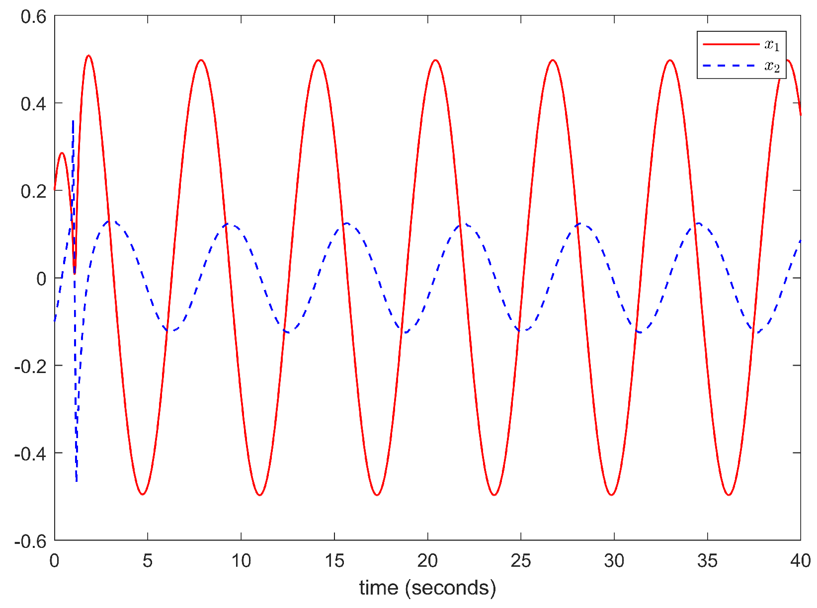
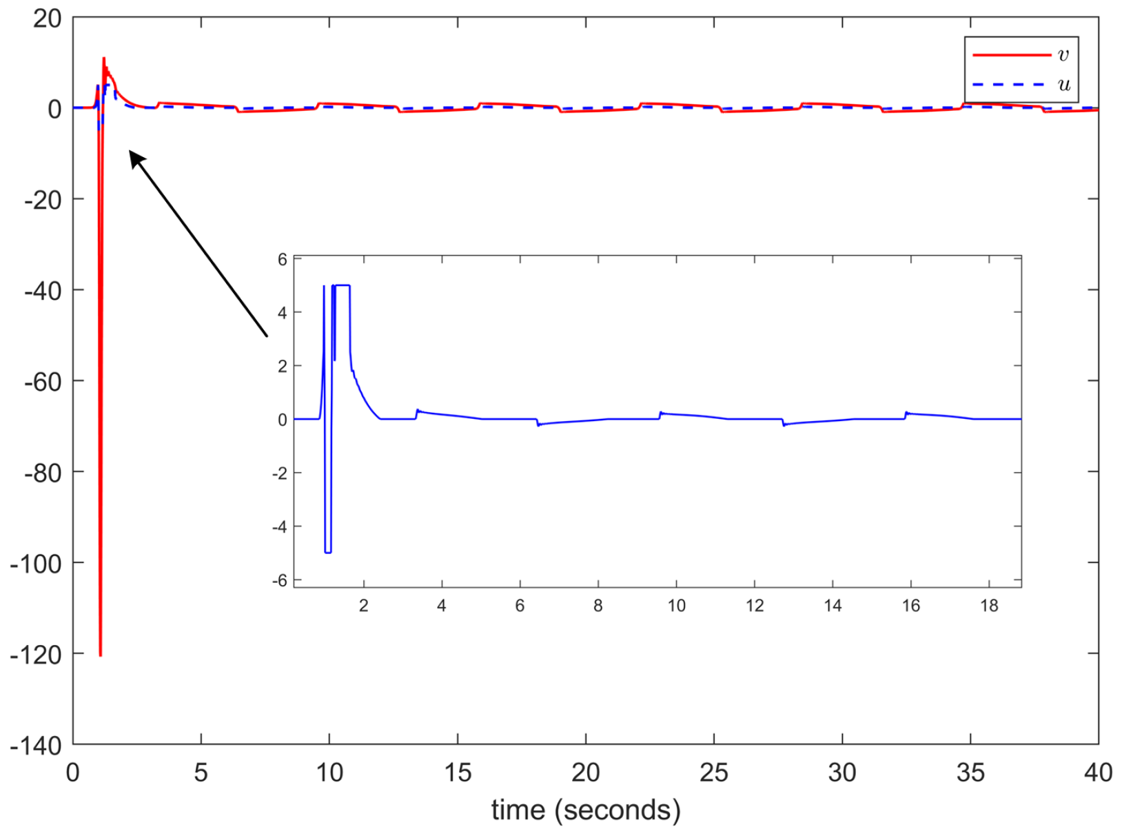
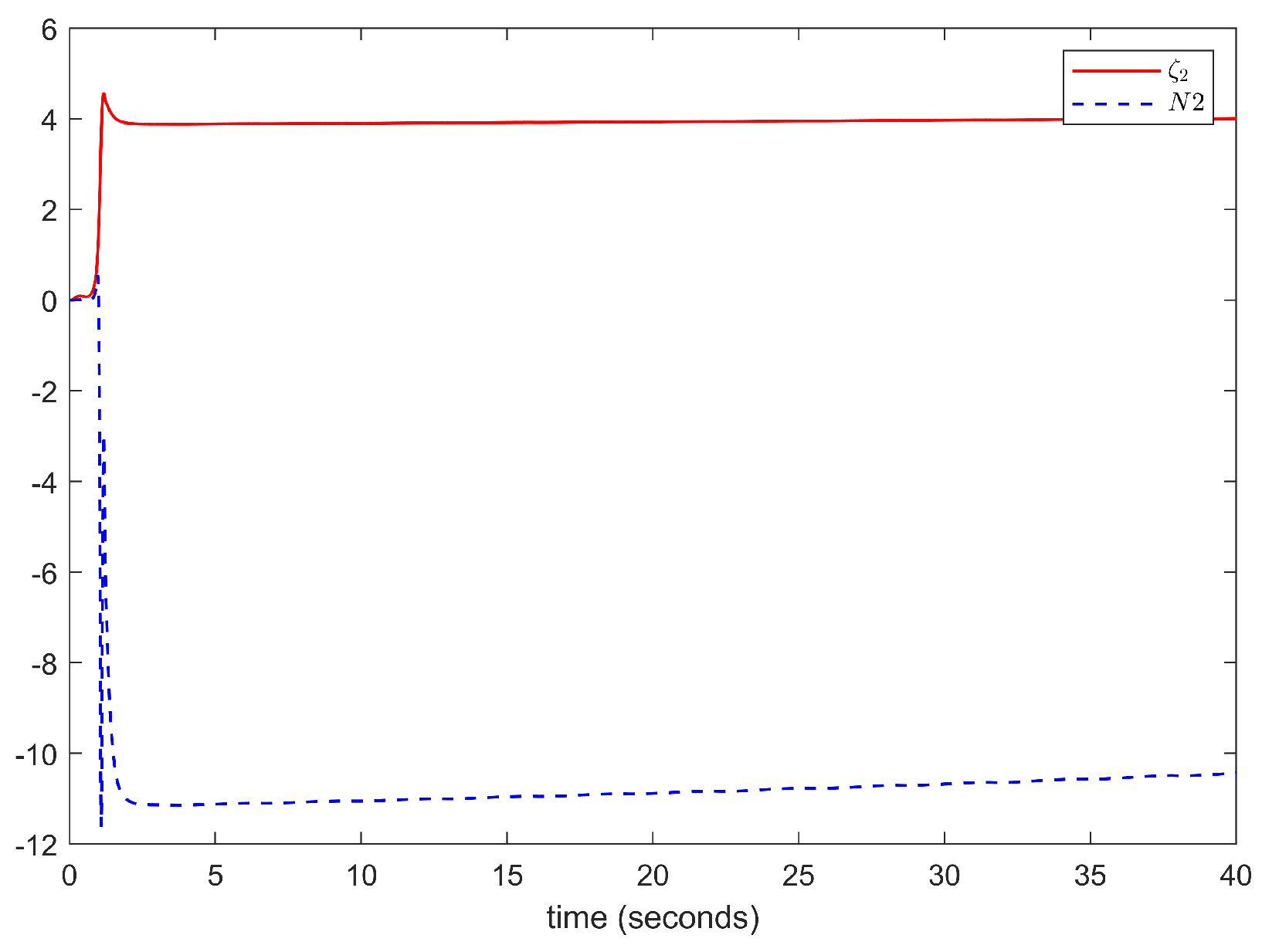
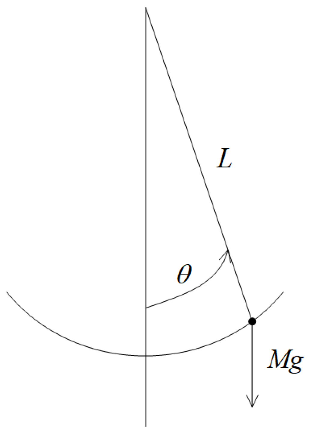
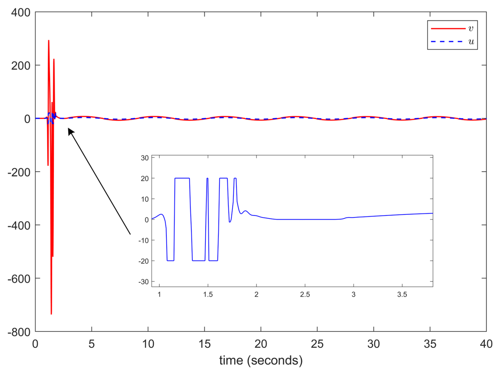
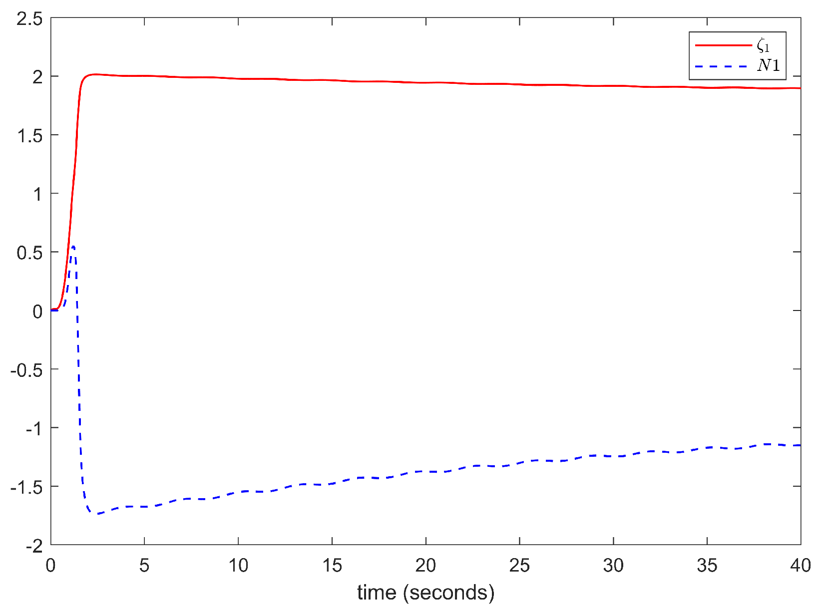
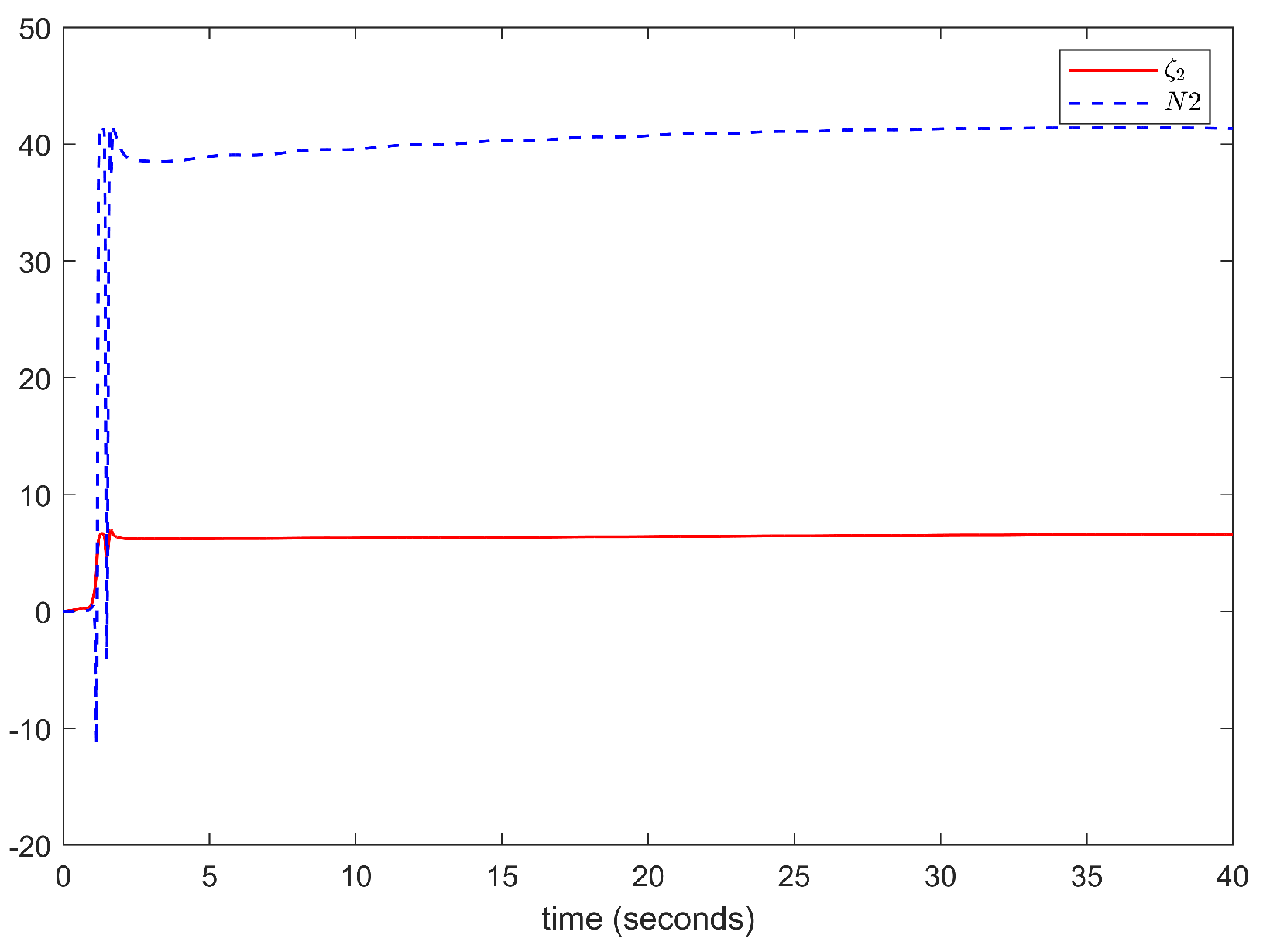
4. Simulation Results

This section provides two illustrative examples to demonstrate the feasibility of the proposed approach.

Example 1.

The following second-order nonlinear system are considered

$$\left\{\begin{array}{c}{\dot{x}}_1=0.1{x_1}^2+{\lambda }_1{g}_1\left({\overline{x}}_1\right)x_2\hfill \\ {\dot{x}}_2=0.2x_1{x}_2+x_1+{\lambda }_2{g}_2\left({\overline{x}}_2\right)u\hfill \\ y=x_1,\hfill \end{array}\right.$$

(54)

where $g_1\left({\overline{x}}_1\right)=4$, $g_2\left({\overline{x}}_2\right)=1$, ${\lambda }_1=-1$, ${\lambda }_2=1$, and u is defined as

$$u=\left\{\begin{array}{cc}5,\hfill & v>5\hfill \\ 0.6\left(v-0.6\right),\hfill & 0.6<v<5\hfill \\ 0,\hfill & -0.6<v<0.6\hfill \\ 0.6\left(v+0.6\right),\hfill & -5<v<0.6\hfill \\ -5,\hfill & v<-5.\hfill \end{array}\right.$$

(55)

The virtual controller ${\alpha }_1$ is designed as

$$\left\{\begin{array}{c}{\alpha }_1=N\left({\zeta }_1\right)\left(\frac{{\xi }_1{\hat{\theta }}_1{\psi }_1^T{\psi }_1}{2a_1^2}+k_1{e}_1+\frac{1}{2}{\xi }_1+\frac{5}{2}{g}_1^2{\xi }_1-{\dot{y}}_d\right),\hfill \\ {\dot{\zeta }}_1={\xi }_1\left(\frac{{\xi }_1{\hat{\theta }}_1{\psi }_1^T{\psi }_1}{2a_1^2}+k_1{e}_1+\frac{1}{2}{\xi }_1+\frac{5}{2}{g}_1^2{\xi }_1-{\dot{y}}_d\right).\hfill \end{array}\right.$$

(56)

The controller v is designed as

$$\left\{\begin{array}{c}v=\frac{1}{\Im }N\left({\zeta }_2\right)\left(\frac{{\xi }_2{\hat{\theta }}_2{\psi }_2^T{\psi }_2}{2a_2^2}+k_2{e}_2+{\xi }_2-{\dot{\omega }}_2\right),\hfill \\ {\dot{\zeta }}_2={\xi }_2\left(\frac{{\xi }_2{\hat{\theta }}_2{\psi }_2^T{\psi }_2}{2a_2^2}+k_2{e}_2+{\xi }_2-{\dot{\omega }}_2\right),\hfill \end{array}\right.$$

(57)

where the initial state variables of the system are $x_1\left(0\right)=0.2$, $x_2\left(0\right)=-0.1$, ${\hat{\theta }}_1\left(0\right)=0.5$, ${\hat{\theta }}_1\left(0\right)=0.2$, and the desired trajectory $y_d=0.5sin\left(t\right)$. The design parameters are given as $k_1=2$, $k_2=1$, $\Im =1$, ${\sigma }_1=0.08$, ${\sigma }_2=0.08$, $a_1=2$, $a_2=7$, ${\mathsf{\Gamma }}_1=0.3$, ${\mathsf{\Gamma }}_2=0.3$, $\varpi =50$, and $\phi =1$ and select $N\left({\zeta }_1\right)={\zeta }_1^{2}cos\left({\zeta }_1\right)$ and $N\left({\zeta }_2\right)={\zeta }_2^{2}cos\left({\zeta }_2\right)$ with ${\zeta }_1\left(0\right)=0$ and ${\zeta }_2\left(0\right)=0$. In addition, to handle nonlinear terms, one might choose the following fuzzy membership function ${\mu }_{P_m^1}=e^{-\frac{{\left(x_1+x_j^0\right)}^2}{2}}$, ${\mu }_{P_m^2}=e^{-\frac{{\left(x_2+x_j^0\right)}^2}{2}}$, ${x_j}^0=3,2,1,0,-1,-2,-3,j=1,\dots 7$.

The simulation results are illustrated in Figure 1, Figure 2, Figure 3, Figure 4, Figure 5 and Figure 6. The trajectories of the system output y and the reference signal $y_d$, using the control strategy proposed in this paper and the control strategy with the same design parameters from reference [27], are shown in Figure 1. According to Figure 1, we can see that the system output y can effectively track the reference signal $y_d$, and the control method proposed in this paper, which accounts for input dead zones and saturation, achieves a higher tracking accuracy compared with the control method proposed in reference [27]. Figure 2 and Figure 3 show states $x_1$ and $x_2$ of the system and the trajectories of the adaptive parameters ${\hat{\theta }}_1$ and ${\hat{\theta }}_2$, respectively. Figure 4 shows the evolution of signals u and v. Figure 5 and Figure 6 describe the Nussbaum function signals ${\zeta }_1$, ${\zeta }_2$, $N\left({\zeta }_1\right)$, and $N\left({\zeta }_2\right)$. Based on the above simulation results, it is evident that the proposed scheme achieves an excellent tracking performance, and all of the signals within the closed-loop system are bounded. This demonstrates the effectiveness of the proposed control scheme.

Example 2.

Consider the pendulum model shown in Figure 7.

Its equation of motion in the tangential direction can be written as

$$ML\ddot{\theta }+kL\dot{\theta }+Mgsin\theta =u,$$

(58)

where $M=1$ denotes the mass of the dot; θ is the angle subtended by the rod and the vertical axis through the pivot point; $k=2$ represents the friction coefficient; $L=1$ is the length of the rod; $g=9.8$ represents the acceleration due to gravity; $\dot{\theta }$ and $\ddot{\theta }$ are angular velocity and angular acceleration, respectively.

Define $x_1=\theta \left(t\right)$ and $x_2=\dot{\theta }\left(t\right)$. Then, the state equations are

$$\left\{\begin{array}{c}{\dot{x}}_1={\lambda }_1{g}_1\left({\overline{x}}_1\right)x_2\hfill \\ {\dot{x}}_2=-2x_2-10sin\left(x_1\right)+{\lambda }_2{g}_2\left({\overline{x}}_1\right)u\hfill \\ y=x_1,\hfill \end{array}\right.$$

(59)

where ${\lambda }_1=1$, ${\lambda }_2=-1$, $g_1\left({\overline{x}}_1\right)=1$, $g_2\left({\overline{x}}_1\right)=1$, and u is defined as

$$u=\left\{\begin{array}{cc}20,\hfill & v>20\hfill \\ 0.5\left(v-0.5\right),\hfill & 0.5<v<20\hfill \\ 0,\hfill & -0.5<v<0.5\hfill \\ 0.5\left(v+0.5\right),\hfill & -20<v<0.5\hfill \\ -20,\hfill & v<-20\hfill \end{array}\right.$$

(60)

The virtual controller, controller, desired signal, Nussbaunm functions, and fuzzy membership function designs are similar to those in Example 1. The initial parameters are chosen as $x_1\left(0\right)=0.2$, $x_2\left(0\right)=-0.1$, ${\hat{\theta }}_1\left(0\right)=0.3$, and ${\hat{\theta }}_1\left(0\right)=0.5$, and the desired trajectory is $y_d=0.5sin\left(t\right)$. The design parameters are $k_1=4$, $k_2=3$, $\Im =1$, ${\sigma }_1=1$, ${\sigma }_2=1$, $a_1=10$, $a_2=10$, ${\mathsf{\Gamma }}_1=0.7$, ${\mathsf{\Gamma }}_2=0.7$, $\varpi =50$, and $\phi =1$.

The simulation results are depicted in Figure 8, Figure 9, Figure 10, Figure 11, Figure 12 and Figure 13. The above simulation results show that the developed adaptive command-filtered fuzzy control scheme achieves a satisfactory tracking performance, with all of the signals in the control system remaining bounded.

5. Conclusions

This paper proposes a command-filtering adaptive fuzzy tracking control strategy for nonlinear systems with unknown control directions, input dead zones, and saturation. A novel approach is applied to analyze the effects of input dead zone and saturation. By combining the fuzzy logic system and the command filter, an adaptive fuzzy logic controller is constructed to ensure that the error signal converges to a bounded compact set around the origin. The combination of the Nussbaum function and the backstepping method solves the difficulty caused by the unknown system control direction. Based on the adaptive tracking controller proposed in this article, the boundedness of all signals in the closed-loop system is guaranteed.

References

1. Xu, H.; Zhu, Q.; Zheng, W.X. Exponential stability of stochastic nonlinear delay systems subject to multiple periodic impulses. IEEE Trans. Autom. Control 2024, 69, 2621–2628. [Google Scholar] [CrossRef]
2. Fan, L.; Zhu, Q.; Zheng, W.X. Stability analysis of switched stochastic nonlinear systems with state-dependent delay. IEEE Trans. Autom. Control 2024, 69, 2567–2574. [Google Scholar] [CrossRef]
3. Zhao, Y.; Zhu, Q. Stabilization of stochastic highly nonlinear delay systems with neutral term. IEEE Trans. Autom. Control 2023, 68, 2544–2551. [Google Scholar] [CrossRef]
4. Do, K.D.; Pan, J. Nonlinear formation control of unicycle-type mobile robots. Robot. Auton. Syst. 2007, 55, 191–204. [Google Scholar] [CrossRef]
5. Merabti, H.; Bouchachi, I.; Belarbi, K. Nonlinear model predictive control of quadcopter. In Proceedings of the 2015 16th International Conference on Sciences and Techniques of Automatic Control and Computer Engineering (STA), Monastir, Tunisia, 21–23 December 2015; IEEE: Piscataway, NJ, USA, 2015; pp. 208–211. [Google Scholar]
6. Geng, X.; Zhan, D.; Zhou, Z. Supervised nonlinear dimensionality reduction for visualization and classification. IEEE Trans. Syst. Man Cybern. Part B Cybern. 2005, 35, 1098–1107. [Google Scholar] [CrossRef]
7. Goege, D.; Fuellekrug, U.; Sinapius, M.; Link, M.; Gaul, L. Advanced test strategy for identification and characterization of nonlinearities of aerospace structures. AIAA J. 2005, 43, 974–986. [Google Scholar] [CrossRef]
8. Liu, Y.; Zhao, W.; Liu, L.; Li, D.; Tong, S.; Chen, C.P. Adaptive neural network control for a class of nonlinear systems with function constraints on states. IEEE Trans. Neural Netw. Learn. Syst. 2021, 34, 2732–2741. [Google Scholar] [CrossRef]
9. Zhang, J.; Niu, B.; Wang, D.; Wang, H.; Duan, P.; Zong, G. Adaptive neural control of nonlinear nonstrict feedback systems with full-state constraints: A novel nonlinear mapping method. IEEE Trans. Neural Netw. Learn. Syst. 2021, 34, 999–1007. [Google Scholar] [CrossRef]
10. Al Mahturi, A.; Santoso, F.; Garratt, M.A.; Anavatti, S.G. A Robust Self-Adaptive Interval Type-2 TS Fuzzy Logic for Controlling Multi-Input–Multi-Output Nonlinear Uncertain Dynamical Systems. IEEE Trans. Syst. Man Cybern. Syst. 2020, 52, 655–666. [Google Scholar] [CrossRef]
11. Park, J.H.; Kim, S.H.; Park, T.S. Output-feedback adaptive neural controller for uncertain pure-feedback nonlinear systems using a high-order sliding mode observer. IEEE Trans. Neural Netw. Learn. Syst. 2018, 30, 1596–1601. [Google Scholar] [CrossRef]
12. Wu, J.; Wu, Z.; Li, J.; Wang, G.; Zhao, H.; Chen, W. Practical adaptive fuzzy control of nonlinear pure-feedback systems with quantized nonlinearity input. IEEE Trans. Syst. Man Cybern. Syst. 2018, 49, 638–648. [Google Scholar] [CrossRef]
13. Li, Y.; Yang, G. Adaptive neural control of pure-feedback nonlinear systems with event-triggered communications. IEEE Trans. Neural Netw. Learn. Syst. 2018, 29, 6242–6251. [Google Scholar] [CrossRef] [PubMed]
14. Swaroop, D.; Hedrick, J.K.; Yip, P.P.; Gerdes, J.C. Dynamic surface control for a class of nonlinear systems. IEEE Trans. Autom. Control 2000, 45, 1893–1899. [Google Scholar] [CrossRef]
15. Zhang, Z.; Wen, C.; Xing, L.; Song, Y. Event-triggered adaptive control for a class of nonlinear systems with mismatched uncertainties via intermittent and faulty output feedback. IEEE Trans. Autom. Control 2023, 68, 8142–8149. [Google Scholar] [CrossRef]
16. Huang, S.; Zong, G.; Wang, H.; Zhao, X.; Alharbi, K.H. Command filter-based adaptive fuzzy self-triggered control for MIMO nonlinear systems with time-varying full-state constraints. Int. J. Fuzzy Syst. 2023, 25, 3144–3161. [Google Scholar] [CrossRef]
17. Yang, Y.; Tang, L.; Zou, W.; Ding, D. Robust adaptive control of uncertain nonlinear systems with unmodeled dynamics using command filter. Int. J. Robust Nonlinear Control 2021, 31, 7764–7784. [Google Scholar] [CrossRef]
18. Wang, L.; Wang, H.; Liu, P.X.; Ling, S.; Liu, S. Fuzzy finite-time command filtering output feedback control of nonlinear systems. IEEE Trans. Fuzzy Syst. 2020, 30, 97–107. [Google Scholar] [CrossRef]
19. Yu, H.; Yu, J.; Wang, Q.; Lin, C. Time-varying BLFs-based adaptive neural network finite-time command-filtered control for nonlinear systems. IEEE Trans. Syst. Man Cybern. Syst. 2023, 53, 4696–4704. [Google Scholar] [CrossRef]
20. Tian, M.; Tao, G. Adaptive dead-zone compensation for output-feedback canonical systems. Int. J. Control 1997, 67, 791–812. [Google Scholar] [CrossRef]
21. Chen, M.; Tao, G. Adaptive fault-tolerant control of uncertain nonlinear large-scale systems with unknown dead zone. IEEE Trans. Cybern. 2015, 46, 1851–1862. [Google Scholar] [CrossRef]
22. Kumar, R.; Singh, U.P.; Bali, A.; Raj, K. Hybrid neural network controller for uncertain nonlinear discrete-time systems with non-symmetric dead zone and unknown disturbances. Int. J. Control 2023, 96, 2003–2011. [Google Scholar] [CrossRef]
23. Tang, F.; Wang, H.; Zhang, L.; Xu, N.; Ahmad, A.M. Adaptive optimized consensus control for a class of nonlinear multi-agent systems with asymmetric input saturation constraints and hybrid faults. Commun. Nonlinear Sci. Numer. Simul. 2023, 126, 107446. [Google Scholar] [CrossRef]
24. Zhao, N.; Tian, Y.; Zhang, H.; Herrera-Viedma, E. Learning-Based Adaptive Fuzzy Output Feedback Control for MIMO Nonlinear Systems With Deception Attacks and Input Saturation. IEEE Trans. Fuzzy Syst. 2024, 32, 2850–2862. [Google Scholar] [CrossRef]
25. Wang, H.; Kang, S.; Zhao, X.; Xu, N.; Li, T. Command filter-based adaptive neural control design for nonstrict-feedback nonlinear systems with multiple actuator constraints. IEEE Trans. Cybern. 2021, 52, 12561–12570. [Google Scholar] [CrossRef]
26. Lu, Y.; Liu, W.; Ma, B. Finite-time command filtered tracking control for time-varying full state-constrained nonlinear systems with unknown input delay. IEEE Trans. Circuits Syst. II Express Briefs 2022, 69, 4954–4958. [Google Scholar] [CrossRef]
27. Xia, J.; Zhang, J.; Feng, J.; Wang, Z.; Zhuang, G. Command filter-based adaptive fuzzy control for nonlinear systems with unknown control directions. IEEE Trans. Syst. Man Cybern. Syst. 2019, 51, 1945–1953. [Google Scholar] [CrossRef]
28. Yang, Y.; Tang, L.; Zou, W.; Ahn, C.K. Novel command-filtered Nussbaum design for continuous-time nonlinear dynamical systems with multiple unknown high-frequency gains. Nonlinear Dyn. 2023, 111, 4313–4323. [Google Scholar] [CrossRef]
29. Yang, Y.; Liu, G.; Li, Q.; Ahn, C.K. Multiple adaptive fuzzy Nussbaum-type functions design for stochastic nonlinear systems with fixed-time performance. Fuzzy Sets Syst. 2024, 476, 108767. [Google Scholar] [CrossRef]
30. Ye, H.; Zhao, K.; Wu, H.; Song, Y. Adaptive control with global exponential stability for parameter-varying nonlinear systems under unknown control gains. IEEE Trans. Cybern. 2023, 53, 7858–7867. [Google Scholar] [CrossRef]
31. Hu, J.; Zhang, H. Immersion and invariance based command-filtered adaptive backstepping control of VTOL vehicles. Automatica 2013, 49, 2160–2167. [Google Scholar] [CrossRef]
Figure 1. Trajectories of y d and y [27].
Mathematics 12 02167 g001
Figure 2. The trajectories of x 1 and x 2 .
Mathematics 12 02167 g002
Figure 3. Adaptive parameters.
Mathematics 12 02167 g003
Figure 4. Trajectories of the control input.
Mathematics 12 02167 g004
Figure 5. The trajectories of ζ 1 and N ( ζ 1 ) .
Mathematics 12 02167 g005
Figure 6. The trajectories of ζ 2 and N ( ζ 2 ) .
Mathematics 12 02167 g006
Figure 7. Pendulum.
Mathematics 12 02167 g007
Figure 8. The trajectories of y d and y.
Mathematics 12 02167 g008
Figure 9. The trajectories of x 1 and x 2 .
Mathematics 12 02167 g009
Figure 10. Adaptive parameters.
Mathematics 12 02167 g010
Figure 11. The trajectories of the control input.
Mathematics 12 02167 g011
Figure 12. The trajectories of ζ 1 and N ( ζ 1 ) .
Mathematics 12 02167 g012
Figure 13. The trajectories of ζ 2 and N ( ζ 2 ) .
Mathematics 12 02167 g013
Disclaimer/Publisher’s Note: The statements, opinions and data contained in all publications are solely those of the individual author(s) and contributor(s) and not of MDPI and/or the editor(s). MDPI and/or the editor(s) disclaim responsibility for any injury to people or property resulting from any ideas, methods, instructions or products referred to in the content.