Numerical Solution to the Time-Fractional Burgers–Huxley Equation Involving the Mittag-Leffler Function

Abstract

Fractional differential equations play a significant role in various scientific and engineering disciplines, offering a more sophisticated framework for modeling complex behaviors and phenomena that involve multiple independent variables and non-integer-order derivatives. In the current research, an effective cubic B-spline collocation method is used to obtain the numerical solution of the nonlinear inhomogeneous time-fractional Burgers–Huxley equation. It is implemented with the help of a $\theta$-weighted scheme to solve the proposed problem. The spatial derivative is interpolated using cubic B-spline functions, whereas the temporal derivative is discretized by the Atangana–Baleanu operator and finite difference scheme. The proposed approach is stable across each temporal direction as well as second-order convergent. The study investigates the convergence order, error norms, and graphical visualization of the solution for various values of the non-integer parameter. The efficacy of the technique is assessed by implementing it on three test examples and we find that it is more efficient than some existing methods in the literature. To our knowledge, no prior application of this approach has been made for the numerical solution of the given problem, making it a first in this regard.

1. Introduction

Fractional calculus is a tool that many researchers employ. A variety of modifications have been made to its usage for relevant operators. Caputo and Fabrizio [1] constructed an innovative operator with an exponential function to tackle the solitary kernel problem. This operator was nonsingular but had a non-locality issue. Atangana and Baleanu [2] established a distinctive operator for fractional derivatives with nonlocal and nonsingular kernels by adopting the generalized Mittag-Leffler function (MLF).

Numerous applications of fractional derivatives may be found in the fields of engineering, biomedicine, control theory, and signal processing [3,4,5]. In recent times, they have been applied to non-Newtonian fluid dynamics, rheology, hysteretic phenomena, geometric approaches, financial systems, and electrochemistry [6,7,8,9,10,11,12]. It is important to learn about the analytical or numerical techniques of solving fractional differential equations (FDEs), as most problems may be expressed by employing them.

Many diverse fields revolve around nonlinear models with temporal fractional derivatives. The generalized Burgers–Huxley equation is a nonlinear partial differential equation that delivers a great description of the interactions in population dynamics, chemical kinetics, reaction diffusion transports, and neurology. The domains in which it is utilized, according to the authors of [13], include engineering, optics, material science, patterned creation, cardiology, and combustion.

A nonlinear inhomogeneous time-fractional Burgers–Huxley equation (TFBHE) is described by:

$$\frac{{\partial }^{\lambda }\widehat{\varphi }}{\partial t^{\lambda }}=\nu \frac{{\partial }^2\widehat{\varphi }}{\partial {\xi }^2}-{\alpha }_1\frac{\partial \widehat{\varphi }}{\partial \xi }\widehat{\varphi }+\beta \widehat{\varphi }(1-{\widehat{\varphi }}^s)({\widehat{\varphi }}^s-\gamma )+F,a\le \xi \le b,t\in [t_0,T],$$

(1)

with respect to an initial condition (IC)

$$\widehat{\varphi }(\xi ,t_0)=ϵ\left(\xi \right),a\le \xi \le b,$$

(2)

and with the boundary conditions (BCs)

$$\widehat{\varphi }(a,t)={\zeta }_1\left(t\right),\widehat{\varphi }(b,t)={\zeta }_2\left(t\right),t\in [t_0,T],$$

(3)

in which $0<\lambda <1$, F is the source term, $\nu >0$ displays viscosity kinematics and the parameters ${\alpha }_1$, $\beta$, $\gamma$ and s follow the conditions $\beta \ge 0$, $\gamma \in (0,1)$, and $s>0$. The term $\frac{{\partial }^{\lambda }}{\partial t^{\lambda }}\widehat{\varphi }(\xi ,t)$ is the Atangana–Baleanu time-fractional derivative (ABTFD).

An approach with tension B-splines was introduced by [14] to solve the Burgers–Huxley equation (BHE). A method with an exact finite difference was developed by [15] to solve the BHE. A linear semi-implicit compact scheme was proposed by [16] to solve the BHE. To find an analytic solution of the BHE, a residual power series method was implemented by [17]. The time-fractional Burgers–Huxley equation (TFBHE) was approximated by [18] using a Lie symmetry analysis method. An Adomian decomposition method was used by Ismail et al. [19] to solve the BHE and Burgers–Fisher equation (BFE). Madiah et al. [20] approximated the time-fractional Burgers equation (TFBE) involving the ABTFD via a cubic B-spline. Jiwari et al. [21] proposed an algorithm based on a weighted average differential quadrature to solve the TFBE. A numerical treatment of the TFBE via a parametric spline was proposed by El-Danaf and Hadoud [22]. Saad et al. [23] applied a new fractional derivative to approximate the Burgers equation (BE). Deniz et al. [24] proposed a Laplace transform optimal perturbation technique to solve a model of a damped BE. A cubic B-spline function collocation technique for time-fractional derivatives was constructed by Majeed et al. [25] to approximate Burgers’s and Fisher’s equation. Khalid et al. [26] solved the Caputo time-fractional Allen–Cahn equation via redefined cubic B-spline functions. Majeed et al. [27] approximated the inhomogeneous TFBHE with B-spline functions and a Caputo derivative. Akram et al. [28] solved the time-fractional Fisher equation via an extended cubic B-spline. Akram et al. [29] used extended cubic B-splines for the solution of the time-fractional telegraph equation. Iqbal et al. [30] used a new quintic polynomial B-spline approximation for the numerical solution of the Kuramoto–Sivashinsky equation. Wang et al. [31] found a new explicit solution of the BHE. Ray et al. [32] solved the BHE and Huxley equation using a wavelet collocation method. Wang [33] presented a variational principle and approximate solution for the generalized Burgers–Huxley equation with fractal derivatives. Sivalingam et al. [34] used a novel L1–Predictor–Corrector method to solve generalized Caputo type fractional differential equations. Sivalingam et al. [35] developed a Chebyshev neural network-based numerical scheme for the solution of distributed-order fractional differential equations. Yuan et al. [36] solved the nonlinear time-fractional Schrödinger equation by constructing linearized transformed $L1$ Galerkin FEMs with unconditional convergence. Yuan et al. [37] used linearized fast time-stepping schemes for time-space fractional Schrödinger equations. Gao et al. [38] solved time-fractional Navier–Stokes equations by using an energy-stable and divergence-free variable-step $L1$ scheme.

This paper is structured as follows: Section 2 exhibits the ABTFD as well as Parseval’s identity and cubic B-spline functions (CBSFs). The latest established methodology is displayed in Section 3. The demonstration of the suggested approach’s stability and convergence is found in Section 4 and Section 5, respectively. Section 6 assesses the efficacy and validity of the suggested strategy, and finally, The conclusion is summed up in Section 7.

2. Preliminaries

Definition 1. 

Suppose that $t>a$, $\lambda >0$, and $\lambda , a, t\in \mathbb{R}$, then the ABTFD of order λ of a function $\widehat{\varphi }\left(t\right)\in H^n(a,b)$, $b>a$ was shown by [20] to be:

$${{}_a{}^{AB}D}_t^{\lambda }\widehat{\varphi }\left(t\right)=\left\{\begin{array}{cc}\hfill \frac{A_B\left(\lambda \right)}{(n-\lambda )}\underset{a}{\overset{t}{\int }}\frac{d^n}{d{\tau }^n}\widehat{\varphi }\left(\tau \right)E_{\lambda }\left[-\frac{\lambda }{n-\lambda }{(t-\tau )}^{\lambda }\right]d\tau ,\hfill & \hfill n-1<\lambda <n\in \mathbb{N},\hfill \\ \hfill \frac{d^n}{d{t}^n}\widehat{\varphi }\left(t\right),\hfill & \hfill \lambda =n\in \mathbb{N},\hfill \end{array}\right.$$

(4)

where $A_B\left(\lambda \right)$ is a function that has been normalized and has the characteristic $A_B(\lambda =0)=1=A_B(\lambda =1)$. $E_{\lambda ,\sigma }\left(t\right)$ is the MLF with $E_{\lambda ,1}\left(t\right)=E_{\lambda }\left(t\right)$, defined as:

$$E_{\lambda ,\sigma }\left(t\right)=\sum _{r=0}^{\infty }\frac{t^r}{\mathsf{\Gamma }(\lambda r+\sigma )}.$$

Definition 2. 

If $\tilde{g}\in L^2[a,b]$, then Parseval’s identity is given by [39]:

$$\sum _{n=-\infty }^{\infty }|\widehat{g}{\left(n\right)|}^2={\int }_a^b{\left|\tilde{g}\left(\xi \right)\right|}^{2}dr,$$

(5)

where $\widehat{g}\left(n\right)={\int }_a^b\tilde{g}\left(\xi \right)e^{2\pi in\xi }d\xi$ is the Fourier transform for every integer n.

Basis Functions for Cubic B-Splines

Let us consider that $a\le \xi \le b$ is to be split with the N equal sized subintervals based on $hN+a=b$ in the sense of $a={\xi }_0, {\xi }_1, \dots , {\xi }_N=b$, where ${\xi }_r<{\xi }_{r+1}$, and ${\xi }_r=hr+{\xi }_0$, $r=0, 1, \dots ,N$.

Now, let $\varphi (\xi ,t)$ be the CBSFs approach for $\widehat{\varphi }(\xi ,t)$ as:

$$\varphi (\xi ,t)=\sum _{r=-1}^{N+1}{\mathsf{\Psi }}_r^m\left(t\right){\widehat{C}}_r\left(\xi \right),$$

(6)

wherein the controlling points represented as ${\mathsf{\Psi }}_r^m\left(t\right)$ need to be determined at each and every temporal stage and the CBSFs are expressed as:

$${\widehat{C}}_r\left(\xi \right)=\frac{1}{6h^3}\left\{\begin{array}{cc}{(\xi -{\xi }_{r-2})}^3,\hfill & \mathrm{if}\xi \in [{\xi }_{r-2},{\xi }_{r-1}),\hfill \\ 3(\xi -{\xi }_{r-1})h^2+3{(\xi -{\xi }_{r-1})}^{2}h-3{(\xi -{\xi }_{r-1})}^3+h^3,\hfill & \mathrm{if}\xi \in [{\xi }_{r-1},{\xi }_r),\hfill \\ 3({\xi }_{r+1}-\xi )h^2+3{(\xi -{\xi }_{r+1})}^{2}h+3{(\xi -{\xi }_{r+1})}^3+h^3,\hfill & \mathrm{if}\xi \in [{\xi }_r,{\xi }_{r+1}),\hfill \\ {({\xi }_{r+2}-\xi )}^3,\hfill & \mathrm{if}\xi \in [{\xi }_{r+1},{\xi }_{r+2}),\hfill \\ 0,\hfill & \mathrm{else}.\hfill \end{array}\right.$$

(7)

The CBSFs preserve a broad range of geometrical features, including symmetrical characteristics, the convex hull features, locally supporting properties, non-negativity, and also a partition of unity [26]. Additionally, ${\widehat{C}}_{-1},{\widehat{C}}_0,\dots ,{\widehat{C}}_{N+1}$ have been established. Equations (6) and (7) give the following estimations

$$\left\{\begin{array}{c}{\left(\varphi \right)}_r^m=\left(\frac{1}{6}\right){\mathsf{\Psi }}_{r-1}^m+\left(\frac{4}{6}\right){\mathsf{\Psi }}_r^m+\left(\frac{1}{6}\right){\mathsf{\Psi }}_{r+1}^m,\hfill \\ {\left({\varphi }_{\xi }\right)}_r^m=\left(\frac{1}{2h}\right){\mathsf{\Psi }}_{r+1}^m+(-\frac{1}{2h}){\mathsf{\Psi }}_{r-1}^m,\hfill \\ {\left({\varphi }_{\xi \xi }\right)}_r^m=\left(\frac{1}{h^2}\right){\mathsf{\Psi }}_{r-1}^m+(-\frac{2}{h^2}){\mathsf{\Psi }}_r^m+\left(\frac{1}{h^2}\right){\mathsf{\Psi }}_{r+1}^m.\hfill \end{array}\right.$$

(8)

3. Illustration of the Scheme

Consider the temporal domain $0\le t\le T$ is to be split into equal lengths of M subintervals based on $\Delta t=\frac{T}{M}$ such as $0=t_0<t_1<,\dots ,<t_M=T$ with the condition $t_m<t_{m+1}$, by taking $m=0,1,\dots ,M$ every $m\Delta t=t_m$. Now, the discretization of ABTFD (1) at $t=t_{m+1}$ with $\lambda \in (0,1)$ is:

$$\begin{array}{ccc}\hfill \frac{{\partial }^{\lambda }}{\partial t^{\lambda }}\widehat{\varphi }(\xi ,t_{m+1})& =& \hfill \frac{A_B\left(\lambda \right)}{1-\lambda }\underset{0}{\overset{t_{m+1}}{\int }}\left(\frac{\partial \widehat{\varphi }(\xi ,\eta )}{\partial \eta }\right)E_{\lambda }\left[-\frac{\lambda {(t_{m+1}-\eta )}^{\lambda }}{1-\lambda }\right]d\eta ,\hfill \\ & =& \hfill \frac{A_B\left(\lambda \right)}{1-\lambda }\sum _{q=0}^m\underset{t_q}{\overset{t_{q+1}}{\int }}\left(\frac{\partial \widehat{\varphi }(\xi ,\eta )}{\partial \eta }\right)E_{\lambda }\left[-\frac{\lambda {(t_{m+1}-\eta )}^{\lambda }}{1-\lambda }\right]d\eta .\hfill \end{array}$$

(9)

Implementing the forward difference formulation, we acquire from Equation (9)

$$\begin{array}{cc}\hfill \frac{{\partial }^{\lambda }}{\partial t^{\lambda }}\widehat{\varphi }(\xi ,t_{m+1})& =\frac{A_B\left(\lambda \right)}{1-\lambda }\sum _{q=0}^m\frac{\widehat{\varphi }(\xi ,t_{q+1})-\widehat{\varphi }(\xi ,t_q)}{\Delta t}\underset{t_q}{\overset{t_{q+1}}{\int }}{E}_{\lambda }\left[-\frac{\lambda {(t_{m+1}-\eta )}^{\lambda }}{1-\lambda }\right]d\eta +R_{\Delta t}^{m+1}\hfill \\ \hfill & =\frac{A_B\left(\lambda \right)}{1-\lambda }\sum _{q=0}^m\left(\widehat{\varphi }(\xi ,t_{m-q+1})-\widehat{\varphi }(\xi ,t_{m-q})\right)\left(\right\{(q+1)E_{\lambda ,2}\left[-\frac{\lambda {\left((q+1)\Delta t\right)}^{\lambda }}{1-\lambda }\right]\hfill \\ \hfill & -q{E}_{\lambda ,2}\left[-\frac{\lambda {(q\Delta t)}^{\lambda }}{1-\lambda }\right])+R_{\Delta t}^{m+1}\hfill \\ \hfill & =\frac{A_B\left(\lambda \right)}{1-\lambda }\sum _{q=0}^m\left(\widehat{\varphi }(\xi ,t_{m-q+1})-\widehat{\varphi }(\xi ,t_{m-q})\right)\left((q+1)E_{q+1}-q{E}_q\right)+R_{\Delta t}^{m+1}.\hfill \end{array}$$

Hence,

$$\frac{{\partial }^{\lambda }}{\partial t^{\lambda }}\widehat{\varphi }(\xi ,t_{m+1})=\frac{A_B\left(\lambda \right)}{1-\lambda }\sum _{q=0}^m{\aleph }_q\left[\widehat{\varphi }(\xi ,t_{m-q+1})-\widehat{\varphi }(\xi ,t_{m-q})\right]+R_{\Delta t}^{m+1},$$

(10)

where $E_q=E_{\lambda ,2}\left[-\frac{\lambda {(q\Delta t)}^{\lambda }}{1-\lambda }\right]$, and ${\aleph }_q=(q+1)E_{q+1}-q{E}_q$. A straightforward observation indicates the following:

• ${\aleph }_q>0$ and ${\aleph }_0=E_1$, $q=0,1,\dots ,m$;
• ${\aleph }_0>{\aleph }_1>{\aleph }_2>,\dots ,>{\aleph }_q,{\aleph }_q\to 0$ as $q\to \infty$;
• ${\sum }_{q=0}^m({\aleph }_q-{\aleph }_{q+1})+{\aleph }_{m+1}=(E_1-{\aleph }_1)+{\sum }_{q=1}^{m-1}({\aleph }_q-{\aleph }_{q+1})+{\aleph }_m=E_1$.

Also, the truncation error $R_{\Delta t}^{m+1}$ is presented in [20] as:

$$\begin{array}{cc}\hfill R_{\Delta t}^{m+1}& =\frac{A_B\left(\lambda \right)}{1-\lambda }\sum _{q=0}^m\underset{t_q}{\overset{t_{q+1}}{\int }}\frac{\Delta t}{2}\frac{{\partial }^2\widehat{\varphi }(\xi ,t_q)}{\partial t^2}{E}_{\lambda }\left[-\frac{\lambda {(t_{m+1}-\eta )}^{\lambda }}{1-\lambda }\right]d\eta \hfill \\ \hfill & =\frac{A_B\left(\lambda \right)}{1-\lambda }\frac{{(\Delta t)}^2}{2}\sum _{q=0}^m\frac{{\partial }^2\widehat{\varphi }(\xi ,t_q)}{\partial t^2}\{(m-q+1)E_{\lambda ,2}\left[-\frac{\lambda {\left((m-q+1)\Delta t\right)}^{\lambda }}{1-\lambda }\right]\hfill \\ \hfill & -(m-q)E_{\lambda ,2}\left[-\frac{\lambda {((m-q)\Delta t)}^{\lambda }}{1-\lambda }\right]\}\hfill \\ \hfill & =\frac{A_B\left(\lambda \right)}{1-\lambda }\frac{{(\Delta t)}^2}{2}\sum _{q=0}^m\frac{{\partial }^2\widehat{\varphi }(\xi ,t_q)}{\partial t^2}\left((m-q+1)E_{m-q+1}-(m-q)E_{m-q}\right)\hfill \\ \hfill & \le \frac{A_B\left(\lambda \right)}{1-\lambda }\frac{{(\Delta t)}^2}{2}\left[\underset{0\le t\le t_m}{max}\frac{{\partial }^2\widehat{\varphi }(\xi ,t)}{\partial t^2}\right]W_1,\hfill \end{array}$$

where $W_1$ is constant.

$$|R_{\Delta t}^{m+1}{| \le (\Delta t)}^2\delta ,$$

(11)

where $\delta$ is constant.

• Simply employing the $\theta$-weighted approach in Equation (10) as well, then Equation (1) turns it into

$$\begin{array}{c}\hfill \frac{A_B\left(\lambda \right)}{1-\lambda }\sum _{q=0}^m{\aleph }_q\left(\varphi (\xi ,t_{m-q+1})-\varphi (\xi ,t_{m-q})\right)=\theta (\nu {\varphi }_{\xi \xi }(\xi ,t_{m+1})-{\alpha }_1{\varphi }_{\xi }(\xi ,t_{m+1})\varphi (\xi ,t_{m+1})\hfill \\ +\beta \varphi (\xi ,t_{m+1})(1-{\varphi }^s(\xi ,t_{m+1}))({\varphi }^s(\xi ,t_{m+1})-\gamma ))\\ +(1-\theta )(\nu {\varphi }_{\xi \xi }(\xi ,t_m)-{\alpha }_1{\varphi }_{\xi }(\xi ,t_m)\varphi (\xi ,t_m)\\ \hfill +\beta \varphi (\xi ,t_m)(1-{\varphi }^s(\xi ,t_m))({\varphi }^s(\xi ,t_m)-\gamma ))+F.\end{array}$$

(12)

The $\theta$-weighted scheme is a numerical method for solving differential equations that provides an adjustable compromise between explicit and implicit time-stepping. When $\theta =1$, the method is fully implicit; when $\theta =0$, it is fully explicit; and when $\theta =0.5$, it follows the Crank–Nicolson approach. Throughout the paper, we use $\theta =1$ in Equation (12) with respect to the direction of space and employ a formula of the linearization displayed in [27] as:

$${\left({\varphi }^s\right)}_r^{m+1}=s{\left(\varphi \right)}_r^{m+1}{\left({\varphi }^{s-1}\right)}_r^m-(s-1){\left({\varphi }^s\right)}_r^m.$$

(13)

$${\left({\varphi }^s{\varphi }_{\xi }\right)}_r^{m+1}=s{\left(\varphi \right)}_r^{m+1}{\left({\varphi }^{s-1}{\varphi }_{\xi }\right)}_r^m+{\left({\varphi }_{\xi }\right)}_r^{m+1}{\left({\varphi }^s\right)}_r^m-s{\left({\varphi }^s{\varphi }_{\xi }\right)}_r^m.$$

(14)

By considering $s=1$, we find that

$$\begin{array}{c}\hfill \left(E_1+{\alpha }_1{a}_1{\left({\varphi }_{\xi }\right)}_r^m-2a_1\beta (1+\gamma ){\left(\varphi \right)}_r^m+a_1\beta \gamma +3a_1\beta {\left({\varphi }^2\right)}_r^m\right){\left(\varphi \right)}_r^{m+1}\hfill \\ +{\alpha }_1{a}_1{\left(\varphi \right)}_r^m{\left({\varphi }_{\xi }\right)}_r^{m+1}-a_1\nu {\left({\varphi }_{\xi \xi }\right)}_r^{m+1}=E_1{\left(\varphi \right)}_r^m+{\alpha }_1{a}_1{\left(\varphi \right)}_r^m{\left({\varphi }_{\xi }\right)}_r^m-a_1\beta (1+\gamma ){\left({\varphi }^2\right)}_r^m+\\ \hfill 2a_1\beta {\left({\varphi }^3\right)}_r^m-\sum _{q=1}^m{\aleph }_q\left({\left(\varphi \right)}_r^{m-q+1}-{\left(\varphi \right)}_r^{m-q}\right)+a_1{F}_r^{m+1},\end{array}$$

(15)

where $a_1=\frac{1-\lambda }{R\left(\lambda \right)}$, ${\varphi }_r^m=\varphi ({\xi }_r,t_m)$, and $F_r^{m+1}=F({\xi }_r,t_{m+1})$.

Utilizing (8) in (15), we acquire

$$\begin{array}{c}\hfill {\mu }_1\left(\frac{1}{6}{\mathsf{\Psi }}_{r-1}^{m+1}+\frac{4}{6}{\mathsf{\Psi }}_r^{m+1}+\frac{1}{6}{\mathsf{\Psi }}_{r+1}^{m+1}\right)+{\mu }_2\left(\frac{-1}{2h}{\mathsf{\Psi }}_{r-1}^{m+1}+\frac{1}{2h}{\mathsf{\Psi }}_{r+1}^{m+1}\right)\hfill \\ -\varsigma \left(\frac{1}{h^2}{\mathsf{\Psi }}_{r-1}^{m+1}-\frac{2}{h^2}{\mathsf{\Psi }}_r^{m+1}+\frac{1}{h^2}{\mathsf{\Psi }}_{r+1}^{m+1}\right)={\mu }_3\left(\frac{1}{6}{\mathsf{\Psi }}_{r-1}^m+\frac{4}{6}{\mathsf{\Psi }}_r^m+\frac{1}{6}{\mathsf{\Psi }}_{r+1}^m\right)\\ \hfill -\sum _{q=1}^m{\aleph }_q\left[\frac{1}{6}\left({\mathsf{\Psi }}_{r-1}^{m-q+1}-{\mathsf{\Psi }}_{r-1}^{m-q}\right)+\frac{4}{6}\left({\mathsf{\Psi }}_r^{m-q+1}-{\mathsf{\Psi }}_r^{m-q}\right)+\frac{1}{6}\left({\mathsf{\Psi }}_{r+1}^{m-q+1}-{\mathsf{\Psi }}_{r+1}^{m-q}\right)\right]+a_1{F}_r^{m+1}.\end{array}$$

(16)

After some simplification, we get

$$\begin{array}{c}\hfill \left(\frac{1}{6}{\mu }_1-\frac{1}{2h}{\mu }_2-\frac{\varsigma }{h^2}\right){\mathsf{\Psi }}_{r-1}^{m+1}+\left(\frac{4}{6}{\mu }_1+\frac{2\varsigma }{h^2}\right){\mathsf{\Psi }}_r^{m+1}+\left(\frac{1}{6}{\mu }_1+\frac{1}{2h}{\mu }_2-\frac{\varsigma }{h^2}\right){\mathsf{\Psi }}_{r+1}^{m+1}=P_r^m\end{array}$$

(17)

The Equation (17) is simplified as:

$$f_r^m{\mathsf{\Psi }}_{r-1}^{m+1}+g_r^m{\mathsf{\Psi }}_r^{m+1}+H_r^m{\mathsf{\Psi }}_{r+1}^{m+1}=P_r^m,r=0,1,\dots ,N,m=0,1,\dots ,M,$$

(18)

where

• ${\mu }_1=E_1+{\alpha }_1{a}_1{\left({\varphi }_{\xi }\right)}_r^m-2a_1\beta (1+\gamma ){\left(\varphi \right)}_r^m+a_1\beta \gamma +3a_1\beta {\left({\varphi }^2\right)}_r^m$,
• ${\mu }_2={\alpha }_1{a}_1{\left(\varphi \right)}_r^m$, $\varsigma =a_1\nu$, $f_r^m=\frac{1}{6}{\mu }_1-\frac{1}{2h}{\mu }_2-\frac{\varsigma }{h^2}$,
• ${\mu }_3=E_1+{\alpha }_1{a}_1{\left({\varphi }_{\xi }\right)}_r^m-a_1\beta (1+\gamma ){\left(\varphi \right)}_r^m+2a_1\beta {\left({\varphi }^2\right)}_r^m$
• $g_r^m=\frac{4}{6}{\mu }_1+\frac{2\varsigma }{h^2}$, $H_r^m=\frac{1}{6}{\mu }_1+\frac{1}{2h}{\mu }_2-\frac{\varsigma }{h^2}$,
• and $P_r^m={\mu }_3[\frac{1}{6}{\mathsf{\Psi }}_{r-1}^m+\frac{4}{6}{\mathsf{\Psi }}_r^m+\frac{1}{6}{\mathsf{\Psi }}_{r+1}^m]$
• $-{\sum }_{q=1}^m{\aleph }_q[\frac{1}{6}({\mathsf{\Psi }}_{r-1}^{m-q+1}-{\mathsf{\Psi }}_{r-1}^{m-q})+\frac{4}{6}({\mathsf{\Psi }}_r^{m-q+1}-{\mathsf{\Psi }}_r^{m-q})+\frac{1}{6}({\mathsf{\Psi }}_{r+1}^{m-q+1}-{\mathsf{\Psi }}_{r+1}^{m-q})]+a_1{F}_r^{m+1}$. System (18) has a total number of $N+3$ unknown but the number of linear equations is $N+1$. From the provided BCs, we also find two equations so that this system can generate a unique solution (3).

$$\left\{\begin{array}{c}\hfill \frac{1}{6}{\mathsf{\Psi }}_{-1}^{m+1}+\frac{4}{6}{\mathsf{\Psi }}_0^{m+1}+\frac{1}{6}{\mathsf{\Psi }}_1^{m+1}={\zeta }_1^{m+1},\hfill \\ \hfill \frac{1}{6}{\mathsf{\Psi }}_{N-1}^{m+1}+\frac{4}{6}{\mathsf{\Psi }}_N^{m+1}+\frac{1}{6}{\mathsf{\Psi }}_{N+1}^{m+1}={\zeta }_2^{m+1}.\hfill \end{array}\right.$$

(19)

The following is the matrix form for Equations (18) and (19):

$$\left(\begin{array}{ccccccc}\frac{1}{6}& \frac{4}{6}& \frac{1}{6}& & & & \\ f_0^m& g_0^m& H_0^m& & & & \\ & f_1^m& g_1^m& H_1^m& & & \\ & & \ddots & \ddots & \ddots & & \\ & & & f_{N-1}^m& g_{N-1}^m& H_{N-1}^m& \\ & & & & f_N^m& g_N^m& H_N^m\\ & & & & \frac{1}{6}& \frac{4}{6}& \frac{1}{6}\end{array}\right)\left(\begin{array}{c}{\mathsf{\Psi }}_{-1}^{m+1}\\ {\mathsf{\Psi }}_0^{m+1}\\ {\mathsf{\Psi }}_1^{m+1}\\ ⋮\\ {\mathsf{\Psi }}_{N-1}^{m+1}\\ {\mathsf{\Psi }}_N^{m+1}\\ {\mathsf{\Psi }}_{N+1}^{m+1}\end{array}\right)=\left(\begin{array}{c}{\zeta }_1^{m+1}\\ P_0^{m+1}\\ P_1^{\widehat{m}+1}\\ ⋮\\ P_{N-1}^{m+1}\\ P_N^{m+1}\\ {\zeta }_2^{m+1}\end{array}\right),$$

(20)

by utilizing the IC as in Equation (2), the initial vector ${\mathsf{\Psi }}^0={[{\mathsf{\Psi }}_{-1}^0,{\mathsf{\Psi }}_0^0,\dots ,{\mathsf{\Psi }}_{N+1}^0]}^T$ is acquired as follows:

$$\left\{\begin{array}{cc}{\left({\mathsf{\Psi }}_{\xi }\right)}_r^0={ϵ}^{\prime }\left({\xi }_r\right),\hfill & r=0,\hfill \\ {\left({\mathsf{\Psi }}_{\xi }\right)}_r^0=ϵ\left({\xi }_r\right),\hfill & r=0,1,\dots ,N,\hfill \\ {\left({\mathsf{\Psi }}_{\xi }\right)}_r^0={ϵ}^{\prime }\left({\xi }_r\right),\hfill & r=N.\hfill \end{array}\right.$$

(21)

For the previously mentioned equation system, the matrix form representation is:

$$U{\mathsf{\Psi }}^0=Q,$$

(22)

where

$$\left(\begin{array}{ccccccc}\frac{-1}{2h}& 0& \frac{1}{2h}& & & & \\ \frac{1}{6}& \frac{4}{6}& \frac{1}{6}& & & & \\ & \frac{1}{6}& \frac{4}{6}& \frac{1}{6}& & & \\ & & \ddots & \ddots & \ddots & & \\ & & & \frac{1}{6}& \frac{4}{6}& \frac{1}{6}& \\ & & & & \frac{1}{6}& \frac{4}{6}& \frac{1}{6}\\ & & & & \frac{-1}{2h}& 0& \frac{1}{2h}\end{array}\right)\left(\begin{array}{c}{\mathsf{\Psi }}_{-1}^0\\ {\mathsf{\Psi }}_0^0\\ {\mathsf{\Psi }}_1^0\\ ⋮\\ {\mathsf{\Psi }}_{N-1}^0\\ {\mathsf{\Psi }}_N^0\\ {\mathsf{\Psi }}_{N+1}^0\end{array}\right)=\left(\begin{array}{c}{ϵ}^{\prime }\left({\xi }_0\right)\\ ϵ\left({\xi }_0\right)\\ ϵ\left({\xi }_1\right)\\ ⋮\\ ϵ\left({\xi }_{N-1}\right)\\ ϵ\left({\xi }_N\right)\\ {ϵ}^{\prime }\left({\xi }_N\right)\end{array}\right).$$

(23)

Equation (23) is solved by any numerical procedure. The numerical findings were conducted in Mathematica 10.

4. The Stability of the Proposed Scheme

When the error never increases during the computing process, the numerical methodology is viewed as stable in [40]. The Fourier methodology [28,29,30] was implemented to ensure the stability of the suggested approach. Now, let ${\tau }_k^m$ and ${\tilde{\tau }}_k^m$ display the amplification component and its estimation in the Fourier transformation. The error ${\kappa }_k^m$ can be tackled by:

$${\kappa }_r^m={\tau }_r^m-{\tilde{\tau }}_r^m,r=1,2,\dots ,N-1,m=1,2,\dots ,M.$$

Putting ($F=0$) in Equation (16) implies:

$$\begin{array}{c}\hfill f_r^m{\mathsf{\Psi }}_{r-1}^{m+1}+g_r^m{\mathsf{\Psi }}_r^{m+1}+H_r^m{\mathsf{\Psi }}_{r+1}^{m+1}={\gamma }_1{\mathsf{\Psi }}_{r-1}^m+{\gamma }_2{\mathsf{\Psi }}_r^m+{\gamma }_3{\mathsf{\Psi }}_{r+1}^m\hfill \\ \hfill -\sum _{q=1}^m{\aleph }_q\left(\frac{1}{6}({\mathsf{\Psi }}_{r-1}^{m-q+1}-{\mathsf{\Psi }}_{r-1}^{m-q})+\frac{4}{6}({\mathsf{\Psi }}_r^{m-q+1}-{\mathsf{\Psi }}_r^{m-q})+\frac{1}{6}({\mathsf{\Psi }}_{r+1}^{m-q+1}-{\mathsf{\Psi }}_{r+1}^{m-q})\right),\end{array}$$

(24)

wherein ${\gamma }_1=\frac{{\mu }_3}{6}$, ${\gamma }_2=\frac{4{\mu }_3}{6}$, ${\gamma }_3=\frac{{\mu }_3}{6}$.

From both IC and BCs, for $r=1,2,\dots ,N$, we have

$${\widehat{\varphi }}_r^0=ϵ\left({\xi }_r\right),$$

(25)

and for $m=0,1,\dots ,M$,

$$\left\{\begin{array}{c}{\mathsf{\Psi }}_0^m={\zeta }_1\left(t_m\right),\hfill \\ {\mathsf{\Psi }}_N^m={\zeta }_2\left(t_m\right).\hfill \end{array}\right.$$

(26)

Define the gridding function as:

$${\mathsf{\Psi }}^m=\left\{\begin{array}{c}{\mathsf{\Psi }}_r^m,\xi \in ({\xi }_r-\frac{h}{2},{\xi }_r+\frac{h}{2}],r=1,2,\dots ,N-1,\hfill \\ 0,\xi \in [a,a+\frac{h}{2}]or\xi \in [b-\frac{h}{2},b].\hfill \end{array}\right.$$

(27)

The presentation in the Fourier mode of ${\mathsf{\Psi }}^m\left(\xi \right)$ is

$${\mathsf{\Psi }}^m\left(\xi \right)=\sum _{n=-\infty }^{\infty }{\widehat{\mathsf{{\rm Y}}}}^m\left(n\right)e^{\frac{2\pi tnr}{b-a}},$$

(28)

where

$${\widehat{\mathsf{{\rm Y}}}}^m\left(n\right)=\frac{1}{b-a}{\int }_a^b{\mathsf{\Psi }}^m\left(r\right)e^{\frac{-2\pi tnr}{b-a}}d\xi ,m=0,1,\dots ,M\mathrm{and}{\mathsf{\Psi }}^m={[{\mathsf{\Psi }}_1^m,{\mathsf{\Psi }}_2^m,\dots ,{\mathsf{\Psi }}_{N-1}^m]}^T.$$

(29)

Employing the norm ${\parallel .\parallel }_2$, we have

$$\begin{array}{cc}\hfill \parallel {\mathsf{\Psi }}^m{\parallel }_2& =\sqrt{h\sum _{r=1}^{N-1}{\left|{\mathsf{\Psi }}_r^m\right|}^2}\hfill \\ \hfill & ={\left({\int }_a^{a+\frac{h}{2}}|{\mathsf{\Psi }}^m{|}^{2}d\xi +\sum _{r=1}^{N-1}{\int }_{{\xi }_k-\frac{h}{2}}^{{\xi }_k+\frac{h}{2}}|{\mathsf{\Psi }}^m{|}^{2}d\xi +{\int }_{b-\frac{h}{2}}^b{|{\mathsf{\Psi }}^m|}^{2}d\xi \right)}^{\frac{1}{2}}\hfill \\ \hfill & ={\left({\int }_a^b{\left|{\mathsf{\Psi }}^m\right|}^{2}d\xi \right)}^{\frac{1}{2}}.\hfill \end{array}$$

From Parseval’s identity (5), we acquire [39]

$${\int }_a^b|{\mathsf{\Psi }}^m{|}^{2}d\xi =\sum _{n=-\infty }^{\infty }{|{\widehat{\mathsf{{\rm Y}}}}^m\left(n\right)|}^2.$$

Therefore, we obtain

$$\parallel {\mathsf{\Psi }}^m{\parallel }_2^2=\sum _{n=-\infty }^{\infty }{|{\widehat{\mathsf{{\rm Y}}}}^m\left(n\right)|}^2.$$

(30)

Suppose the solution in the Fourier mode of Equations (24)–(26) is

$${\mathsf{\Psi }}_r^m={\widehat{\mathsf{{\rm Y}}}}^m{e}^{i\alpha rh},$$

(31)

where i represents $\sqrt{-1}$ and displaying $\alpha$ as real. Employing Equation (31) in Equation (24), we acquire

$$\begin{array}{c}{f}_r^m{\widehat{\mathsf{{\rm Y}}}}^{m+1}{e}^{-i\alpha h}+g_r^m{\widehat{\mathsf{{\rm Y}}}}^{m+1}+H_r^m{\widehat{\mathsf{{\rm Y}}}}^{m+1}{e}^{i\alpha h}={\gamma }_1{\widehat{\mathsf{{\rm Y}}}}^m{e}^{-i\alpha h}+{\gamma }_2{\widehat{\mathsf{{\rm Y}}}}^m+{\gamma }_3{\widehat{\mathsf{{\rm Y}}}}^m{e}^{i\alpha h}\hfill \\ -{\displaystyle \sum _{q=1}^m}{\aleph }_q\left(\frac{1}{6}({\widehat{\mathsf{{\rm Y}}}}^{m-q+1}{e}^{-i\alpha h}-{\widehat{\mathsf{{\rm Y}}}}^{m-q}{e}^{-i\alpha h})+\frac{4}{6}({\widehat{\mathsf{{\rm Y}}}}^{m-q+1}-{\widehat{\mathsf{{\rm Y}}}}^{m-q})+\frac{1}{6}({\widehat{\mathsf{{\rm Y}}}}^{m-q+1}{e}^{i\alpha h}-{\widehat{\mathsf{{\rm Y}}}}^{m-q}{e}^{i\alpha h})\right),\hfill \end{array}$$

(32)

Applying the result $\frac{e^{2i\alpha h}+1}{2e^{i\alpha h}}=cos\left(\alpha h\right)$ and also using $f_r^m$, $g_r^m$, $H_r^m$, the following equality is obtained:

$${\widehat{\mathsf{{\rm Y}}}}^{m+1}=\frac{{\widehat{\mathsf{{\rm Y}}}}^m{\mu }_{3}A}{A{\mu }_1+\frac{iB{\mu }_2}{h}-\frac{2\varsigma C}{h^2}}-\frac{A{\sum }_{q=1}^m{\aleph }_q\left({\widehat{\mathsf{{\rm Y}}}}^{m-q+1}-{\widehat{\mathsf{{\rm Y}}}}^{m-q}\right)}{A{\mu }_1+\frac{iB{\mu }_2}{h}-\frac{2\varsigma C}{h^2}},$$

(33)

$${\widehat{\mathsf{{\rm Y}}}}^{m+1}=\frac{A{\mu }_3(A{\mu }_1-\frac{iB{\mu }_2}{h}-\frac{2\varsigma C}{h^2})}{{(A{\mu }_1-\frac{2\varsigma C}{h^2})}^2+{\left(\frac{{\mu }_{2}B}{h}\right)}^2}\left({\widehat{\mathsf{{\rm Y}}}}^m-\frac{{\sum }_{q=1}^m{\aleph }_q\left({\widehat{\mathsf{{\rm Y}}}}^{m-q+1}-{\widehat{\mathsf{{\rm Y}}}}^{m-q}\right)}{{\mu }_3}\right),$$

(34)

$${\widehat{\mathsf{{\rm Y}}}}^{m+1}=\frac{{\widehat{\mathsf{{\rm Y}}}}^m}{\sigma }-\sum _{q=1}^m{\aleph }_q\frac{{\widehat{\mathsf{{\rm Y}}}}^{m-q+1}-{\widehat{\mathsf{{\rm Y}}}}^{m-q}}{{\mu }_3\sigma },$$

(35)

where $\sigma =\frac{{(A{\mu }_1-\frac{2\varsigma C}{h^2})}^2+{\left(\frac{{\mu }_{2}B}{h}\right)}^2}{A{\mu }_3(A{\mu }_1-\frac{iB{\mu }_2}{h}-\frac{2\varsigma C}{h^2})}$, $A=\frac{2cos\left(\alpha h\right)+4}{6}$, $B=sin\left(\alpha h\right)$, and $C=cos\left(\alpha h\right)-1$. Obviously, $\sigma \ge 1$ and ${\mu }_3>0$.

Lemma 1. 

If ${\widehat{\mathsf{{\rm Y}}}}^m$ is the solution of Equation (35), then $|{\widehat{\mathsf{{\rm Y}}}}^m| \le |{\widehat{\mathsf{{\rm Y}}}}^0|,m=0,1,\dots ,M$.

Proof. 

Using the method of mathematical induction to prove the lemma, when $m=0$, Equation (35) gives

$$|{\widehat{\mathsf{{\rm Y}}}}^1| =\frac{1}{\sigma }|{\widehat{\mathsf{{\rm Y}}}}^0| \le |{\widehat{\mathsf{{\rm Y}}}}^0|,\sigma \ge 1.$$

Let us suppose that $|{\widehat{\mathsf{{\rm Y}}}}^m| \le |{\widehat{\mathsf{{\rm Y}}}}^0|$ for $m=1,2,\dots ,M-1$, then

$$\begin{array}{cc}\hfill |{\widehat{\mathsf{{\rm Y}}}}^{m+1}|& \le \frac{1}{\sigma }\left|{\widehat{\mathsf{{\rm Y}}}}^m\right|-\frac{1}{\sigma {\mu }_3}\sum _{q=1}^m{\aleph }_q\left(|{\widehat{\mathsf{{\rm Y}}}}^{m-q+1}|-|{\widehat{\mathsf{{\rm Y}}}}^{m-q}|\right)\hfill \\ \hfill & \le \frac{1}{\sigma }\left|{\widehat{\mathsf{{\rm Y}}}}^0\right|-\frac{1}{\sigma {\mu }_3}\sum _{q=1}^m{\aleph }_q\left(|{\widehat{\mathsf{{\rm Y}}}}^0|-|{\widehat{\mathsf{{\rm Y}}}}^0|\right)\hfill \\ \hfill & \le |{\widehat{\mathsf{{\rm Y}}}}^0|.\hfill \end{array}$$

□

Theorem 1. 

The proposed technique in Equation (18) is unconditionally stable.

Proof. 

Applying Lemma (1) and Equation (30), we obtain

$${\parallel \mathsf{\Psi }m\parallel }_{ 2}\le {\left|{\mathsf{\Psi }}^0\right|}_2,\forall m=0,1,\dots ,M.$$

This lemma demonstrates the unconditional stability of the suggested technique. □

5. Convergence of the Developed Scheme

The methodology from [41] is used to analyze the convergence of the propagated approach. We start with the following theorem [42,43].

Theorem 2. 

Consider F belonging in $C^2[a,b]$, $\varphi (\xi ,t)$ relating to $C^4[a,b]$, and take the partition of $a\le \xi \le b$ as $\mho =\{a={\xi }_0,{\xi }_1,\dots ,{\xi }_N=b\}$ in such a way that ${\xi }_r<{\xi }_{r+1}$ is based on ${\xi }_r-a=hr$, where $r=0,1,\dots ,N$. If the unique spline interpolates the solution curve, $\tilde{\varphi }(\xi ,t)$ for ${\xi }_r\in \mho$, then at each and every $t\ge 0$, there is a constant ${\varpi }_r$ independent of h, obtained for $r=0,1,2.$

$$\parallel D^r\left(\tilde{\varphi }(\xi ,t)-\varphi (\xi ,t)\right){\parallel }_{\infty }\le {\varpi }_r{h}^{4-r}$$

(36)

Lemma 2. 

As the CBSFs $\{{\widehat{C}}_{-1},{\widehat{C}}_0,\dots ,{\widehat{C}}_{N+1}\}$ in Equation (7) fulfils the inequality given in [20],

$$\sum _{k=-1}^{N+1}\left|{\widehat{C}}_{\widehat{k}}\left(\xi \right)\right|\le \frac{5}{3},0\le \xi \le 1.$$

(37)

Theorem 3. 

The numerical approach $\varphi (\xi ,t)$ for the analytic solution $\widehat{\varphi }(\xi ,t)$ for TFBHE (1), (2), (3) exists. Also, if F belongs to $C^2[0,1]$, then

$$\parallel \widehat{\varphi }{(\xi ,t)-\varphi (\xi ,t)\parallel }_{\infty }\le \tilde{\varpi }{h}^2,forall0\le t,$$

(38)

when h is appropriately small, but $\tilde{\varpi }$ does not depend on h, such as $\tilde{\varpi }>0$.

Proof. 

Let $\tilde{\varphi }(\xi ,t)={\sum }_{r=-1}^{N+1}{V}_r^m\left(t\right){\widehat{C}}_r\left(\xi \right)$ be the estimated spline for $\varphi (\xi ,t)$. Employing the triangular inequality, we obtain

$$\parallel \varphi (\xi ,t)-\widehat{\varphi }{(\xi ,t)\parallel }_{\infty }\le \parallel \varphi (\xi ,t)-\tilde{\varphi }{(xi,t)\parallel }_{\infty }+{\parallel \tilde{\varphi }(\xi ,t)-\varphi (\xi ,t)\parallel }_{\infty }.$$

From Theorem 2, we have:

$$\parallel \varphi (\xi ,t)-\widehat{\varphi }{(r,t)\parallel }_{\infty }\le {\varpi }_0{h}^4+{\parallel \tilde{\varphi }(\xi ,t)-\varphi (\xi ,t)\parallel }_{\infty }.$$

(39)

For $r=0,1,\dots ,N$ in the suggested method, these $L\varphi ({\xi }_r,t)=L\widehat{\varphi }({\xi }_r,t)=F({\xi }_r,t)$ are the collocation conditions. Considering

$$L\tilde{\varphi }(\xi ,t)=\tilde{F},$$

$L(\tilde{\varphi }({\xi }_r,t)-\varphi ({\xi }_r,t))$ may be derived at any time range as:

$$\begin{array}{c}\hfill \left(\frac{{\mu }_1}{6}+\frac{{\mu }_2}{2h}-\frac{\varsigma }{h^2}\right){\mathsf{\Omega }}_{r-1}^{m+1}+\left(\frac{4{\mu }_1}{6}+\frac{2\varsigma }{h^2}\right){\mathsf{\Omega }}_r^{m+1}+\left(\frac{{\mu }_1}{6}-\frac{{\mu }_2}{2h}-\frac{\varsigma }{h^2}\right){\mathsf{\Omega }}_{r+1}^{m+1}\hfill \\ =\frac{{\mu }_3}{6}{\mathsf{\Omega }}_{r-1}^m+\frac{4{\mu }_3}{6}{\mathsf{\Omega }}_r^m-\frac{{\mu }_3}{6}{\mathsf{\Omega }}_{r+1}^m)+\frac{a_1}{h^2}{\rho }_r^{m+1}\\ \hfill -\sum _{q=1}^m{\aleph }_q\left[\frac{1}{6}({\mathsf{\Omega }}_{r-1}^{m-q+1}-{\mathsf{\Omega }}_{r-1}^{m-q})+\frac{4}{6}({\mathsf{\Omega }}_r^{m-q+1}-{\mathsf{\Omega }}_r^{m-q})+\frac{1}{6}({\mathsf{\Omega }}_{r+1}^{m-q+1}-{\mathsf{\Omega }}_{r+1}^{m-q})\right].\end{array}$$

(40)

The description of the BCs is

$$\frac{1}{6}{\mathsf{\Omega }}_{r-1}^{m+1}+\frac{4}{6}{\mathsf{\Omega }}_r^{m+1}+\frac{1}{6}{\mathsf{\Omega }}_{r+1}^{m+1}=0,r=0,N.$$

For $r=-1,0,\dots ,N+1$,

$${\mathsf{\Omega }}_r^m={\mathsf{\Psi }}_r^m-V_r^m,$$

and for $r=0,1,\dots ,N$,

$${\rho }_r^m=[F_r^m-{\tilde{F}}_r^m]h^2,$$

now, using inequality (36),

$$|{\rho }_r^m|=h^2|F_r^m-{\tilde{F}}_r^m|\le \varpi h^4.$$

Defining ${\rho }^m=max\left\{\right|{\rho }_r^m|;r=0,1,\dots ,N\}$, ${\epsilon }_r^m=\left|{\mathsf{\Omega }}_r^m\right|$, and ${\epsilon }^m=max\left\{\right|{\epsilon }_r^m|;0\le r\le N\}.$ When $m=0$, Equation (40) becomes

$$\begin{array}{cc}\hfill & \left(\frac{{\mu }_1}{6}+\frac{{\mu }_2}{2h}-\frac{\varsigma }{h^2}\right){\mathsf{\Omega }}_{r-1}^1+\left(\frac{4{\mu }_1}{6}+\frac{2\varsigma }{h^2}\right){\mathsf{\Omega }}_r^1+\left(\frac{{\mu }_1}{6}-\frac{{\mu }_2}{2h}-\frac{\varsigma }{h^2}\right){\mathsf{\Omega }}_{r+1}^1\hfill \\ \hfill & =\frac{{\mu }_3}{6}{\mathsf{\Omega }}_{r-1}^0+\frac{4{\mu }_3}{6}{\mathsf{\Omega }}_r^0+\frac{{\mu }_3}{6}{\mathsf{\Omega }}_{r+1}^0+\frac{a_1}{h^2}{\rho }_r^1,\hfill \end{array}$$

employing the IC as ${\epsilon }^0=0$. Also, using norms on ${\mathsf{\Omega }}_r^1$ and ${\rho }_r^1$ for small values as well as h, then we obtain

$${\epsilon }_r^1\le \frac{3a_1}{{\mu }_1{h}^2+12\varsigma -3{\mu }_{2}h}\varpi h^4,r=0,1,\dots ,N.$$

We obtain $e_{-1}^1$ and $e_{N+1}^1$ through the BCs

$${\epsilon }_{-1}^1\le \frac{15a_1}{{\mu }_1{h}^2+12\varsigma -3{\mu }_{2}h}\varpi h^4,$$

$${\epsilon }_{N+1}^1\le \frac{15a_1}{{\mu }_1{h}^2+12\varsigma -3{\mu }_{2}h}\varpi h^4,$$

which implies

$${\epsilon }^1\le {\varpi }_1{h}^2,$$

(41)

wherein ${\varpi }_1$ does not depend on h.

• Now, we employ the procedure of mathematical induction to prove the theorem on m. Let ${\epsilon }_r^i\le {\varpi }_i{h}^2$ be true by taking $i=1\left(2\right)m$ with $\varpi =max\{{\varpi }_i:0\le i\le m\}$; then, we obtain from Equation (40) the following:

$$\begin{array}{c}\left(\frac{{\mu }_1}{6}+\frac{{\mu }_2}{2h}-\frac{\varsigma }{h^2}\right){\mathsf{\Omega }}_{r-1}^{m+1}+\left(\frac{4{\mu }_1}{6}+\frac{2\varsigma }{h^2}\right){\mathsf{\Omega }}_r^{m+1}+\left(\frac{{\mu }_1}{6}-\frac{{\mu }_2}{2h}-\frac{\varsigma }{h^2}\right){\mathsf{\Omega }}_{r+1}^{m+1}\hfill \\ =[({\aleph }_0-{\aleph }_1)\left(\frac{1}{6}{\mathsf{\Omega }}_{r-1}^m+\frac{4}{6}{\mathsf{\Omega }}_r^m+\frac{1}{6}{\mathsf{\Omega }}_{r+1}^m\right)+({\aleph }_1-{\aleph }_2)\left(\frac{1}{6}{\mathsf{\Omega }}_{r-1}^{m-1}+\frac{4}{6}{\mathsf{\Omega }}_r^{m-1}+\frac{1}{6}{\mathsf{\Omega }}_{r+1}^{m-1}\right)+\hfill \\ +({\aleph }_{m-1}-{\aleph }_m)\left(\frac{1}{6}{\mathsf{\Omega }}_{r-1}^1+\frac{4}{6}{\mathsf{\Omega }}_r^1+\frac{1}{6}{\mathsf{\Omega }}_{r+1}^1\right)+{\aleph }_m\left(\frac{1}{6}{\mathsf{\Omega }}_{r-1}^0+\frac{4}{6}{\mathsf{\Omega }}_r^0+\frac{1}{6}{\mathsf{\Omega }}_{r+1}^0\right)]+\frac{a_1}{h^2}{\rho }_r^{m+1}.\hfill \end{array}$$

Again, using norms on ${\mathsf{\Omega }}_r^m$ and ${\rho }_r^m$, we obtain

$${\epsilon }_r^{m+1}\le \frac{3\varpi h^4}{{\mu }_1{h}^2+12\varsigma -3{\mu }_{2}h}\left(a_1+\sum _{v=0}^{m-1}({\aleph }_q-{\aleph }_{q+1})\right).$$

Similarly, we have the values of ${\epsilon }_{-1}^{m+1}$ and ${\epsilon }_{N+1}^{m+1}$ from the BCs

$${\epsilon }_{-1}^{m+1}\le \frac{15\varpi h^4}{{\mu }_1{h}^2+12\varsigma -3{\mu }_{2}h}\left(a_1+\sum _{q=0}^{m-1}({\aleph }_q-{\aleph }_{q+1})\right),$$

$${\epsilon }_{N+1}^{m+1}\le \frac{15\varpi h^4}{{\mu }_1{h}^2+12\varsigma -3{\mu }_{2}h}\left(a_1+\sum _{q=0}^{m-1}({\aleph }_q-{\aleph }_{q+1})\right).$$

So for every m,

$${\epsilon }^{m+1}\le \varpi h^2.$$

(42)

In particular,

$$\tilde{\varphi }(\xi ,t)-\varphi (\xi ,t)=\sum _{r=-1}^{N+1}\left(V_r\left(t\right)-{\mathsf{\Psi }}_r\left(t\right)\right){\widehat{C}}_r\left(\xi \right).$$

Therefore, from Lemma (2) and inequality (42), we obtain

$$\parallel \tilde{\varphi }{(\xi ,t)-\varphi (\xi ,t)\parallel }_{\infty }\le \frac{5}{3}\varpi h^2.$$

(43)

Employing (43), the inequality (39) becomes

$${\parallel \varphi (\xi ,t)-\varphi (\xi ,t)\parallel }_{\infty }\le {\varpi }_0{h}^4+\frac{5}{3}\varpi h^2=\tilde{\varpi }{h}^2,$$

where $\tilde{\varpi }={\varpi }_0{h}^2+\frac{5}{3}\varpi$. □

Theorem 4. 

The TFBHE converges with respect to both the BCs as well as the IC.

Proof. 

Let $\widehat{\varphi }(\xi ,t)$ be the analytical result for the TFBHE and $\varphi (\xi ,t)$ be the estimated solutions. Thus, the theorem mentioned above together with relation (11) support the existence of constants δ and $\tilde{\varpi }$ such that

$$\parallel \widehat{\varphi (\xi ,t)-\varphi }{(\xi ,t)\parallel }_{\infty }\le \tilde{\varpi }{h}^2+{(\Delta t)}^2\delta .$$

Hence, the rate of convergence in both temporal and spatial dimensions is the second order of the suggested method. □

6. Analysis and Presentation of Numerical Examples

This section presents a numerical solution of the TFBHE using cubic B-spline functions for different values of the fractional-order derivative $\lambda$. The numerical results are shown graphically and numerically in the form of figures and tables. The suggested method’s accuracy is demonstrated numerically in this part using $L_2$ and $L_{\infty }$, which are defined as:

$$\wp =L_2={\parallel \widehat{\varphi }({\xi }_r,t)-\varphi ({\xi }_r,t)\parallel }_2=\sqrt{h\sum _{r=0}^N{|\widehat{\varphi }({\xi }_r,t)-\varphi ({\xi }_r,t)|}^2},$$

$$\Im =L_{\infty }=\parallel \widehat{\varphi }({\xi }_r,t)-\varphi ({\xi }_r,t){\parallel }_{\infty }=\underset{0\le r\le N}{max}|\widehat{\varphi }({\xi }_r,t)-\varphi ({\xi }_r,t)|$$

Hence, the following formula [20,44] is used to compute the order of convergence

$${log}_2\left(\frac{L_{\infty }\left(N\right)}{L_{\infty }\left(2N\right)}\right),$$

where $L_{\infty }\left(N\right)$ and $L_{\infty }\left(2N\right)$ are the absolute errors with the number of partitions N and $2N$, respectively. $A_B\left(\lambda \right)=1$ is taken into consideration for each case.

Example 1. 

Consider the TFBHE for $s=1$

$$\frac{{\partial }^{\lambda }\widehat{\varphi }}{\partial t^{\lambda }}=\nu \frac{{\partial }^2\widehat{\varphi }}{\partial {\xi }^2}-{\alpha }_1\frac{\partial \widehat{\varphi }}{\partial \xi }\widehat{\varphi }+\beta \widehat{\varphi }(1-\widehat{\varphi })(\widehat{\varphi }-\gamma )+F,0\le t\le T,0\le \xi \le 1,$$

with respect to the IC and the BCs

$$\widehat{\varphi }(\xi ,0)=0,0\le \xi \le 1,$$

$$\widehat{\varphi }(0,t)=0,\widehat{\varphi }(1,t)=\frac{t^3}{2},0\le t\le T,$$

and the source term F is

$$\begin{array}{c}\hfill F=6sin\left[\frac{5\xi \pi }{6}\right]t^3{E}_{\lambda ,4}\left[\frac{-\lambda t^{\lambda }}{1-\lambda }\right]+{\alpha }_1{t}^6\frac{5\pi }{6}cos\left[\frac{5\xi \pi }{6}\right]sin\left[\frac{5\xi \pi }{6}\right]+{\left[\frac{5\pi }{6}\right]}^2{t}^{3}sin\left[\frac{5\xi \pi }{6}\right]\hfill \\ \hfill \hspace{1em}\hspace{1em}\hspace{1em}\hspace{1em}\hspace{1em}\hspace{1em}\hspace{1em}\hspace{1em}-\beta \left[t^{3}sin\left(\frac{5\xi \pi }{6}\right)\right]\left[1-t^{3}sin\left(\frac{5\xi \pi }{6}\right)\right]\left[t^{3}sin\left(\frac{5\xi \pi }{6}\right)-\gamma \right].\end{array}$$

$\widehat{\varphi }(\xi ,t)=t^{3}sin\left(\frac{5\pi \xi }{6}\right)$ represents the analytic solution. The representation of the estimated results with absolute errors in Table 1 and Table 2 is based on $\Delta t=0.0002$ and $t=1$ by taking various values of $\lambda$. Table 3 displays the error norms for a range of time intervals and $\lambda$ choices. Table 4 and Table 5 show the ordered process of convergence with the help of error norms in both spatial as well as temporal directions. As shown in Figure 1, for diverse values of time t with $\Delta t=0.0005$, the outcome of the suggested approach and the analytical solution are a close match. The numerical and analytical findings are plotted in three dimensions in Figure 2 for $N=500$, $\Delta t=0.0004$, $\lambda =0.6$, $t=1$, and $\xi \in [0,1]$. At $t=1$, the 2D and 3D error graphs are displayed in Figure 3.

Table 1. For Example 1, the error norms are based on $\Delta t=0.0002$ and $N=500$ by taking various values of $\lambda$.

		$\mathit{\varphi }$		Absolute Error
$\mathit{\xi }$	$\widehat{\mathit{\varphi }}$	$\mathit{\lambda }=\mathbf{0.35}$	$\mathit{\lambda }=\mathbf{0.7}$	$\mathit{\lambda }=\mathbf{0.35}$	$\mathit{\lambda }=\mathbf{0.7}$
0.1	$0.258819$	$0.258819$	$0.258819$	$4.1182\times {10}^{-7}$	$3.91313\times {10}^{-7}$
0.2	$0.5$	$0.499999$	$0.499999$	$7.87686\times {10}^{-7}$	$7.48644\times {10}^{-7}$
0.3	$0.707107$	$0.707106$	$0.707106$	$1.09335\times {10}^{-6}$	$1.03958\times {10}^{-6}$
0.4	$0.866025$	$0.866024$	$0.866024$	$1.30184\times {10}^{-6}$	$1.23855\times {10}^{-6}$
0.5	$0.965926$	$0.965924$	$0.965924$	$1.39555\times {10}^{-6}$	$1.32876\times {10}^{-6}$
0.6	1	$0.999999$	$0.999999$	$1.36484\times {10}^{-6}$	$1.30084\times {10}^{-6}$
0.7	$0.965926$	$0.965925$	$0.965925$	$1.20562\times {10}^{-6}$	$1.15058\times {10}^{-6}$
0.8	$0.866025$	$0.866024$	$0.866025$	$9.18678\times {10}^{-7}$	$8.78141\times {10}^{-7}$
0.9	$0.707107$	$0.707106$	$0.707106$	$5.11325\times {10}^{-7}$	$4.8973\times {10}^{-7}$

Table 2. Error norms for Example 1 at $t=1$ based on $\Delta t=0.0002$.

		$\mathit{\varphi }$		Absolute Error
$\mathit{\xi }$	$\widehat{\mathit{\varphi }}$	$\mathit{\lambda }=\mathbf{0.35}, \mathit{N}=\mathbf{200}$	$\mathit{\lambda }=\mathbf{0.7}, \mathit{N}=\mathbf{250}$	$\mathit{\lambda }=\mathbf{0.35}, \mathit{N}=\mathbf{200}$	$\mathit{\lambda }=\mathbf{0.7}, \mathit{N}=\mathbf{250}$
0.1	$0.258819$	$0.258817$	$0.258817$	$2.48892\times {10}^{-6}$	$1.58995\times {10}^{-6}$
0.2	$0.5$	$0.499995$	$0.499997$	$4.76629\times {10}^{-6}$	$3.04445\times {10}^{-6}$
0.3	$0.707107$	$0.7071$	$0.707103$	$6.62846\times {10}^{-6}$	$4.23323\times {10}^{-6}$
0.4	$0.866025$	$0.866017$	$0.86602$	$7.91022\times {10}^{-6}$	$5.05094\times {10}^{-6}$
0.5	$0.965926$	$0.965917$	$0.96592$	$8.49819\times {10}^{-6}$	$5.42558\times {10}^{-6}$
0.6	1	$0.999992$	$0.999995$	$8.32592\times {10}^{-6}$	$5.31518\times {10}^{-6}$
0.7	$0.965926$	$0.965918$	$0.965921$	$7.36368\times {10}^{-6}$	$4.70093\times {10}^{-6}$
0.8	$0.866025$	$0.86602$	$0.866022$	$5.61553\times {10}^{-6}$	$3.58522\times {10}^{-6}$
0.9	$0.707107$	$0.707104$	$0.707105$	$3.12771\times {10}^{-6}$	$1.99715\times {10}^{-6}$

Table 3. The errors denoted by ℑ and ℘ with various values of $\lambda$ based on $\Delta t=\frac{1}{2000}$, $N=175$, and $0\le \xi \le 1$ for Example 1.

	ℑ		℘
$\mathit{t}$	$\mathit{\lambda }=\mathbf{0.35}$	$\mathit{\lambda }=\mathbf{0.7}$	$\mathit{\lambda }=\mathbf{0.35}$	$\mathit{\lambda }=\mathbf{0.7}$
0.1	$1.12882\times {10}^{-8}$	$1.00085\times {10}^{-8}$	$8.05702\times {10}^{-9}$	$7.14935\times {10}^{-9}$
0.5	$1.46583\times {10}^{-6}$	$1.35493\times {10}^{-6}$	$1.04549\times {10}^{-6}$	$9.66869\times {10}^{-7}$
0.9	$8.80657\times {10}^{-6}$	$8.3244\times {10}^{-6}$	$6.28781\times {10}^{-6}$	$5.94565\times {10}^{-6}$

Table 4. The order of convergence based on $\Delta t=\frac{1}{m}$ obtained for a fixed $h=\frac{1}{1000}$ by taking $t=1$ for Example 1.

		Proposed Method
$\mathbf{\lambda }$	$\mathit{m}$	ℑ	℘	Order
0.3	30	$0.000822458$	$0.000557203$	⋯
	60	$0.000228404$	$0.000154969$	$1.84836$
	120	$0.0000599544$	$0.0000406978$	$1.92965$
	240	$0.0000151303$	$0.0000102643$	$1.98643$
	480	$3.56763\times {10}^{-6}$	$2.41059\times {10}^{-6}$	$2.0844$
0.7	30	$0.000828889$	$0.000562391$	⋯
	60	$0.000228405$	$0.000155125$	$1.85958$
	120	$0.000059742$	$0.0000405856$	$1.93478$
	240	$0.000015058$	$0.0000102227$	$1.98821$
	480	$3.55732\times {10}^{-6}$	$2.40571\times {10}^{-6}$	$2.08167$

Table 5. For a fixed $\Delta t=\frac{1}{1000}$, convergence order for Example 1 based on $h=\frac{1}{n}$ with $t=1$.

		Proposed Method
$\mathit{\lambda }$	$\mathit{n}$	ℑ	℘	Order
0.35	10	$0.00357057$	$0.00256221$	⋯
	20	$0.000894128$	$0.000641119$	$1.9976$
	40	$0.000223469$	$0.000159881$	$2.00041$
	80	$0.0000551941$	$0.0000395113$	$2.01749$
	160	$0.0000131207$	$9.41541\times {10}^{-6}$	$2.07267$
0.7	10	$0.00340736$	$0.00244646$	⋯
	20	$0.000853492$	$0.000612011$	$1.99721$
	40	$0.000213221$	$0.000152596$	$2.00103$
	80	$0.0000526365$	$0.0000376926$	$2.01821$
	160	$0.0000124866$	$8.96387\times {10}^{-6}$	$2.07568$

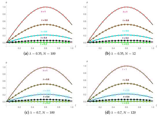
Figure 1. Analytical and approximate results for Example 1 at various temporal scales with $\Delta t=0.0005$.

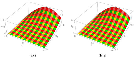
Figure 2. For Example 1, where $0\le \xi \le 1$, 3D analytical solution and numerical solution images with $N=500$, $t=1$, $\lambda =0.6$, and $\Delta t=0.0004$.

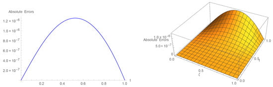
Figure 3. With $N=500$, $t=1$, $\lambda =0.6$, and $\Delta t=0.0004$ for Example 1, 2D and 3D error visuals when $1\le \xi \le 1$.

Example 2. 

Consider the TFBHE for $s=1$

$$\frac{{\partial }^{\lambda }\widehat{\varphi }}{\partial t^{\lambda }}=\nu \frac{{\partial }^2\widehat{\varphi }}{\partial {\xi }^2}-{\alpha }_1\frac{\partial \widehat{\varphi }}{\partial \xi }\widehat{\varphi }+\beta \widehat{\varphi }(1-\widehat{\varphi })(\widehat{\varphi }-\gamma )+F,0\le t\le T,0\le \xi \le 1,$$

with respect to the IC and the BCs

$$\widehat{\varphi }(\xi ,0)=0,0\le \xi \le 1$$

$$\widehat{\varphi }(0,t)=t^3,\widehat{\varphi }(1,t)=exp\left(1\right)t^3,0\le t\le T,$$

and the source term F is

$$\begin{array}{c}\hfill F=6exp\left({\xi }^2\right)t^3{E}_{\lambda ,4}\left[\frac{-\lambda t^{\lambda }}{1-\lambda }\right]-2[t^{3}exp\left({\xi }^2\right)][1+2{\xi }^2]\hfill \\ \hfill +2\xi {\alpha }_1{[t^{3}exp\left({\xi }^2\right)]}^2-\beta [t^{3}exp\left({\xi }^2\right)][1-t^{3}exp\left({\xi }^2\right)][t^{3}exp\left({\xi }^2\right)-\gamma ].\end{array}$$

$\widehat{\varphi }(\xi ,t)=t^{3}exp\left({\xi }^2\right)$ represents the exact solution. For Example 2, the estimated outcomes with absolute errors based on $\Delta t=0.0002$ and $t=1$ by setting $N=500,200,250$ for different values of $\lambda$ are shown in Table 6 and Table 7. For diverse value of t with $N=500$ based on $\Delta t=0.0005$ by varying $\lambda$, Table 8 exhibits the error norms. In both temporal and spatial directions, the ordering of convergence is established in Table 9 and Table 10. The performance of the analytical results and the numerical results at various temporal directions are revealed in Figure 4. The exact and computational solution is illustrated in three-dimensional visualizations in Figure 5. Figure 6 exhibits the 2D and 3D error plots.

Table 6. For Example 2, the errors norm based on $\lambda$ with $\Delta t=0.0002$, $N=500$, and $t=1$.

		$\mathit{\varphi }$		Absolute Error
$\mathit{\xi }$	$\widehat{\mathit{\varphi }}$	$\mathit{\lambda }=\mathbf{0.35}$	$\mathit{\lambda }=\mathbf{0.7}$	$\mathit{\lambda }=\mathbf{0.35}$	$\mathit{\lambda }=\mathbf{0.7}$
0.1	$1.01005$	$1.01005$	$1.01005$	$2.86337\times {10}^{-7}$	$2.75455\times {10}^{-7}$
0.2	$1.04081$	$1.04081$	$1.04081$	$5.41003\times {10}^{-7}$	$5.20529\times {10}^{-7}$
0.3	$1.09417$	$1.09417$	$1.09417$	$7.62998\times {10}^{-7}$	$7.34921\times {10}^{-7}$
0.4	$1.17351$	$1.17351$	$1.17351$	$9.47227\times {10}^{-7}$	$9.14104\times {10}^{-7}$
0.5	$1.28403$	$1.28402$	$1.28402$	$1.0837\times {10}^{-6}$	$1.04851\times {10}^{-6}$
0.6	$1.43333$	$1.43333$	$1.43333$	$1.156\times {10}^{-6}$	$1.12195\times {10}^{-6}$
0.7	$1.63232$	$1.63232$	$1.63232$	$1.1385\times {10}^{-6}$	$1.10885\times {10}^{-6}$
0.8	$1.89648$	$1.89648$	$1.89648$	$9.91296\times {10}^{-7}$	$9.69103\times {10}^{-7}$
0.9	$2.24791$	$2.24791$	$2.24791$	$6.49704\times {10}^{-7}$	$6.37592\times {10}^{-7}$

Table 7. Errors of Example 2 by taking $\Delta t=0.0002$ with a fixed $t=1$ based on $\Delta t=\frac{1}{2000}$.

		$\mathit{\varphi }$		Absolute Error
$\mathit{\xi }$	$\widehat{\mathit{\varphi }}$	$\mathit{\lambda }=\mathbf{0.35}, \mathit{N}=\mathbf{200}$	$\mathit{\lambda }=\mathbf{0.7}, \mathit{N}=\mathbf{250}$	$\mathit{\lambda }=\mathbf{0.35}, \mathit{N}=\mathbf{200}$	$\mathit{\lambda }=\mathbf{0.7}, \mathit{N}=\mathbf{250}$
0.1	$1.01005$	$1.01005$	$1.01005$	$2.04763\times {10}^{-6}$	$1.24276\times {10}^{-6}$
0.2	$1.04081$	$1.04081$	$1.04081$	$3.87188\times {10}^{-6}$	$2.34921\times {10}^{-6}$
0.3	$1.09417$	$1.09417$	$1.09417$	$5.46728\times {10}^{-6}$	$3.31963\times {10}^{-6}$
0.4	$1.17351$	$1.1735$	$1.17351$	$6.79985\times {10}^{-6}$	$4.13554\times {10}^{-6}$
0.5	$1.28403$	$1.28402$	$1.28402$	$7.80097\times {10}^{-6}$	$4.75576\times {10}^{-6}$
0.6	$1.43333$	$1.43332$	$1.43332$	$8.35513\times {10}^{-6}$	$5.10866\times {10}^{-6}$
0.7	$1.63232$	$1.63231$	$1.63231$	$8.27728\times {10}^{-6}$	$5.07778\times {10}^{-6}$
0.8	$1.89648$	$1.89647$	$1.89648$	$7.26857\times {10}^{-6}$	$4.47419\times {10}^{-6}$
0.9	$2.24791$	$2.2479$	$2.24791$	$4.82226\times {10}^{-6}$	$2.97801\times {10}^{-6}$

Table 8. The errors ℑ and ℘ for Example 2 based on $\lambda$ by taking $\Delta t=0.0005$, $N=175$ in $0\le \xi \le 1$.

	ℑ		℘
$\mathit{t}$	$\mathit{\lambda }=\mathbf{0.35}$	$\mathit{\lambda }=\mathbf{0.7}$	$\mathit{\lambda }=\mathbf{0.35}$	$\mathit{\lambda }=\mathbf{0.7}$
0.1	$1.31844\times {10}^{-8}$	$1.18153\times {10}^{-8}$	$9.45187\times {10}^{-9}$	$8.42652\times {10}^{-9}$
0.5	$1.73105\times {10}^{-6}$	$1.60795\times {10}^{-6}$	$1.24234\times {10}^{-6}$	$1.1505\times {10}^{-6}$
0.9	$8.96116\times {10}^{-6}$	$8.57318\times {10}^{-6}$	$6.46477\times {10}^{-6}$	$6.17495\times {10}^{-6}$

Table 9. For Example 2, rate of convergence order by taking $\Delta t=\frac{1}{m}$ with $h=0.001$ at $t=1$.

		Proposed Method
$\mathbf{\lambda }$	$\mathit{m}$	ℑ	℘	Order
0.3	30	$0.00530113$	$0.00380461$	⋯
	60	$0.00142369$	$0.00102271$	$1.89666$
	120	$0.000369471$	$0.00026552$	$1.94611$
	240	$0.0000939479$	$0.0000675277$	$1.97553$
	480	$0.000023468$	$0.0000168677$	$2.00117$
0.7	30	$0.00509274$	$0.003641$	⋯
	60	$0.00136707$	$0.000978226$	$1.89736$
	120	$0.000354643$	$0.000253874$	$1.94665$
	240	$0.0000901537$	$0.0000645476$	$1.97591$
	480	$0.0000225144$	$0.0000161182$	$2.00154$

Table 10. Convergence order of Example 2 by taking $h=\frac{1}{n}$ based on $\Delta t=0.001$ at $t=1$.

		Proposed Method
$\mathit{\lambda }$	$\mathit{n}$	ℑ	℘	Order
0.3	10	$0.00345744$	$0.00252115$	⋯
	20	$0.000859796$	$0.000622447$	$2.00764$
	40	$0.00021041$	$0.00015234$	$2.03079$
	80	$0.0000484937$	$0.0000350984$	$2.11733$
	160	$8.04039\times {10}^{-6}$	$5.80985\times {10}^{-6}$	$2.59246$
0.7	10	$0.00335099$	$0.00244454$	⋯
	20	$0.00083494$	$0.000603534$	$2.00484$
	40	$0.000204384$	$0.00014775$	$2.03039$
	80	$0.0000471449$	$0.0000340841$	$2.11611$
	160	$7.88182\times {10}^{-6}$	$5.68944\times {10}^{-6}$	$2.5805$

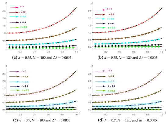
Figure 4. The analytic and approximation solutions for Example 2 at several time ranges.

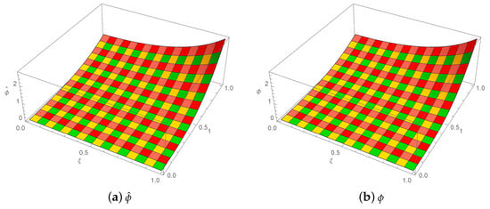
Figure 5. The 3D analytical and numerical solution visuals for Example 2 generated with $N=500$, $t=1$, $\lambda =0.6$, $\Delta t=0.0004$, and $0\le \xi \le 1$.

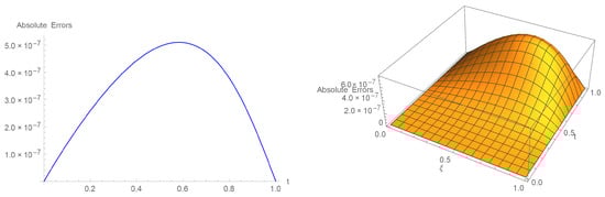
Figure 6. For Example 2, when $0\le \xi \le 1$, 2D and 3D error plots with $N=500$, $t=1$, $\lambda =0.6$, and $\Delta t=0.0004$.

Example 3. 

Consider the TFBHE for $s=1$

$$\frac{{\partial }^{\lambda }\widehat{\varphi }}{\partial t^{\lambda }}=\nu \frac{{\partial }^2\widehat{\varphi }}{\partial {\xi }^2}-{\alpha }_1\frac{\partial \widehat{\varphi }}{\partial \xi }\widehat{\varphi }+\beta \widehat{\varphi }(1-\widehat{\varphi })(\widehat{\varphi }-\gamma )+F,0\le t\le T,0\le \xi \le 1,$$

with respect to both IC and BCs

$$\widehat{\varphi }(\xi ,0)=0,0\le \xi \le 1,$$

$$\widehat{\varphi }(0,t)=0,\widehat{\varphi }(1,t)=0,0\le t\le T,$$

and the source term F is

$$\begin{array}{c}\hfill F=(\xi -{\xi }^2)t^{2\lambda }\mathsf{\Gamma }(2\lambda +1)E_{\lambda ,2\lambda +1}\left[\frac{-\lambda t^{\lambda }}{1-\lambda }\right]+{\alpha }_1(\xi -{\xi }^2)(1-2\xi )t^{4\lambda }\hfill \\ \hfill +2t^{2\lambda }-\beta \left[(\xi -{\xi }^2)t^{2\lambda }\right][1-(\xi -{\xi }^2)t^{2\lambda }][(\xi -{\xi }^2)t^{2\lambda }-\gamma ].\end{array}$$

$\widehat{\varphi }(\xi ,t)=t^{2\lambda }(\xi -{\xi }^2)$ exhibits an analytical solution. The computational outcomes with absolute errors are displayed in Table 11 and Table 12 of Example 3 based on various $\lambda$, $\Delta t=0.001$, taking $t=1$ and $N=100$, 60, and 80. Based on $N=100$, $\Delta t=0.001$, and $\xi \in [0,1]$, the error norms for distinct values of t are presented in Table 13 for many different values of $\lambda$. Table 14 described the comparison with [27]. Table 15 and Table 16 demonstrate the convergent rate. The illustration of exact as well as computational outcome at various time scales is given in Figure 7. The diagram of both the numerical as well as analytical findings in the Figure 8 illustrate the 3D accuracy of the current methodology. The efficacy of the technique is demonstrated by 2D as well as 3D error summaries in Figure 9. Figure 10 displays 2D plots of errors norm and computational outcomes with $t=0.5$, $N=100$, and $\Delta t=0.01$ establishing various values of $\lambda$, such as 3.

Table 11. Absolute errors of Example 3 by setting $\Delta t=\frac{1}{1000}$ based on $N=100$ at $t=1$ with $\lambda$.

	$\mathit{\lambda }=0.6$			$\mathit{\lambda }=0.9$
$\mathit{\xi }$	$\widehat{\mathit{\varphi }}$	$\mathit{\varphi }$	Error	$\widehat{\mathit{\varphi }}$	$\mathit{\varphi }$	Error
0.1	$0.09$	$0.08999$	$1.34250\times {10}^{-9}$	$0.09$	0.09000	$5.80468\times {10}^{-9}$
0.2	$0.16$	$0.15999$	$2.61957\times {10}^{-9}$	$0.16$	0.16000	$1.08216\times {10}^{-8}$
0.3	$0.21$	$0.20999$	$3.67178\times {10}^{-9}$	$0.21$	0.21000	$1.46479\times {10}^{-8}$
0.4	$0.24$	$0.23999$	$4.36309\times {10}^{-9}$	$0.24$	0.24000	$1.70348\times {10}^{-8}$
0.5	$0.25$	$0.24999$	$4.61606\times {10}^{-9}$	$0.25$	0.25000	$1.78202\times {10}^{-8}$
0.6	$0.24$	$0.23999$	$4.40270\times {10}^{-9}$	$0.24$	0.24000	$1.69534\times {10}^{-8}$
0.7	$0.21$	$0.20999$	$3.73745\times {10}^{-9}$	$0.21$	0.21000	$1.45127\times {10}^{-8}$
0.8	$0.16$	$0.15999$	$2.68768\times {10}^{-9}$	$0.16$	0.16000	$1.06811\times {10}^{-8}$
0.9	$0.09$	$0.08999$	$1.38631\times {10}^{-9}$	$0.09$	0.09000	$5.71415\times {10}^{-9}$

Table 12. Errors for Example 3 based on $\Delta t=0.001$ by taking $t=1$.

	$\mathit{\lambda }=0.6,\mathit{N}=60$			$\mathit{\lambda }=0.9,\mathit{N}=80$
$\mathit{\xi }$	$\widehat{\mathit{\varphi }}$	$\mathit{\varphi }$	Absolute Error	$\widehat{\mathit{\varphi }}$	$\mathit{\varphi }$	Absolute Error
0.1	$0.09$	$0.08999$	$1.34242\times {10}^{-9}$	$0.09$	0.09000	$5.80429\times {10}^{-9}$
0.2	$0.16$	$0.15999$	$2.61926\times {10}^{-9}$	$0.16$	0.16000	$1.08210\times {10}^{-8}$
0.3	$0.21$	$0.20999$	$3.67127\times {10}^{-9}$	$0.21$	0.21000	$1.464722\times {10}^{-8}$
0.4	$0.24$	$0.23999$	$4.36248\times {10}^{-9}$	$0.24$	0.24000	$1.70341\times {10}^{-8}$
0.5	$0.25$	$0.24999$	$4.61542\times {10}^{-9}$	$0.25$	0.25000	$1.78194\times {10}^{-8}$
0.6	$0.24$	$0.23999$	$4.40208\times {10}^{-9}$	$0.24$	0.24000	$1.69526\times {10}^{-8}$
0.7	$0.21$	$0.20999$	$3.73692\times {10}^{-9}$	$0.21$	0.21000	$1.45120\times {10}^{-8}$
0.8	$0.16$	$0.15999$	$2.68734\times {10}^{-9}$	$0.16$	0.16000	$1.06805\times {10}^{-8}$
0.9	$0.09$	$0.08999$	$1.38621\times {10}^{-9}$	$0.09$	0.09000	$5.71377\times {10}^{-9}$

Table 13. For Example 3, error norms based on $\Delta t=\frac{1}{1000}$ by taking $\lambda$ with $N=100$ at $0\le \xi \le 1$.

	ℑ		℘
$\mathit{t}$	$\mathit{\lambda }=\mathbf{0.6}$	$\mathit{\lambda }=\mathbf{0.9}$	$\mathit{\lambda }=\mathbf{0.6}$	$\mathit{\lambda }=\mathbf{0.9}$
0.1	$1.88597\times {10}^{-11}$	$2.42752\times {10}^{-10}$	$1.40194\times {10}^{-11}$	$1.72703\times {10}^{-10}$
0.5	$9.89340\times {10}^{-10}$	$6.80308\times {10}^{-9}$	$6.82408\times {10}^{-10}$	$4.85148\times {10}^{-9}$
0.9	$3.84309\times {10}^{-9}$	$1.54587\times {10}^{-8}$	$2.68818\times {10}^{-9}$	$1.10531\times {10}^{-8}$

Table 14. Error norm comparison for Example 3 based on $\lambda =0.6$, $N=100$, and $k=1000$ when $0\le \xi \le 1$.

	Ref. [27]		Proposed Method
$\mathit{t}$	ℑ	℘	ℑ	℘
0.25	$1.069\times {10}^{-6}$	$1.02\times {10}^{-5}$	$6.74962\times {10}^{-11}$	$1.01699\times {10}^{-10}$
0.5	$4.826\times {10}^{-6}$	$3.7\times {10}^{-5}$	$6.82405\times {10}^{-10}$	$9.89337\times {10}^{-10}$
0.75	$5.0\times {10}^{-8}$	$3.0\times {10}^{-7}$	$1.84958\times {10}^{-9}$	$2.65682\times {10}^{-9}$
1	$1.62\times {10}^{-5}$	$1.1\times {10}^{-4}$	$3.24020\times {10}^{-9}$	$4.61607\times {10}^{-9}$

Table 15. For a fixed value of $h=\frac{1}{1000}$, rate of convergence order of Example 3 based on $\Delta t=\frac{1}{m}$ at $t=1$.

		Proposed Method
$\mathit{\lambda }$	$\mathit{m}$	ℑ	℘	Order
0.6	30	$5.42789\times {10}^{-6}$	$3.80853\times {10}^{-6}$	⋯
	60	$1.33075\times {10}^{-6}$	$9.33961\times {10}^{-7}$	$2.02815$
	120	$3.28237\times {10}^{-7}$	$2.30387\times {10}^{-7}$	$2.01943$
	240	$8.12601\times {10}^{-8}$	$5.70367\times {10}^{-8}$	$2.01412$
	480	$2.01641\times {10}^{-8}$	$1.4153\times {10}^{-8}$	$2.01076$
0.9	30	$0.0000191$	$0.0000137$	⋯
	60	$4.8559766\times {10}^{-6}$	$3.4674771\times {10}^{-6}$	$1.9821412$
	120	$1.2197232\times {10}^{-6}$	$8.7078107\times {10}^{-7}$	$1.9932076$
	240	$3.0565195\times {10}^{-6}$	$2.1818752\times {10}^{-7}$	$1.9965921$
	480	$7.6573994\times {10}^{-8}$	$5.4658742\times {10}^{-8}$	$1.9969633$

Table 16. Convergence order based on $h=\frac{1}{n}$ with $\Delta t=\frac{1}{m}$ for Example 3 at $t=1$.

		Proposed Method
$\mathit{\lambda }$	$\mathit{n}=\mathit{m}$	ℑ	℘	Order
0.6	10	$0.0000511$	$0.0000358$	⋯
	20	$0.0000123$	$8.6863473\times {10}^{-6}$	$2.04641$
	40	$3.0239680\times {10}^{-6}$	$2.1222930\times {10}^{-6}$	$2.03360$
	80	$7.4379116\times {10}^{-7}$	$5.2209184\times {10}^{-7}$	$2.02347$
	160	$1.8381158\times {10}^{-7}$	$1.2901980\times {10}^{-7}$	$2.01667$
0.9	10	$0.0001608$	$0.0001150$	⋯
	20	$0.0000424$	$0.0000303$	$1.92104$
	40	$0.00001085$	$7.7495415\times {10}^{-6}$	$1.96928$
	80	$2.7369664\times {10}^{-6}$	$1.9542175\times {10}^{-6}$	$1.98709$
	160	$6.8685893\times {10}^{-7}$	$4.9034940\times {10}^{-7}$	$1.99449$

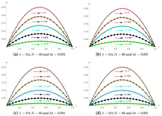
Figure 7. The analytical and numerical solutions in different temporal directions for Example 3.

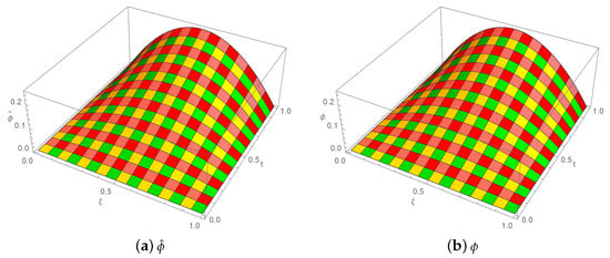
Figure 8. When $0\le \xi \le 1$, 3D analytical solution and numerical solution visuals for Example 3 with $N=500$, $t=1$, $\lambda =0.6$, and $\Delta t=0.0004$.

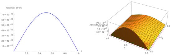
Figure 9. The 2D and 3D error visualizations for Example 3 where $N=500$, $t=1$, $\lambda =0.6$, $\Delta t=0.0004$, and $0\le \xi \le 1$.

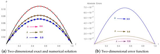
Figure 10. Example 3: 2D impact of fractional parameter when $N=100$, $t=0.5$, $\Delta t=0.01$, and $0\le \xi \le 1$.

7. Conclusions

In the current research, an effective approach to the TFBHE with the ABTFD was proposed using a numerical technique based on CBSFs. The standard finite difference formulation was employed to approximate the ABTFD, and the solution curve was then interpolated in the spatial direction using CBSFs. The method used in this study is new and provides a respectable degree of accuracy. The modified linearization formula was applied to many nonlinear terms, and it was found that this formula could be used to linearize any nonlinear term. The suggested strategy exhibited second-order temporal and spatial convergence and was unconditionally stable. Numerical examples indicated that the current technique was more effective, simple, and widely accepted. Future research should expand the scope, analyze algorithm features, and explore real-world applications, as well as investigate Atangana–Baleanu derivatives’ applications in a coupled system of partial differential equations.

References

- Caputo, M.; Fabrizio, M. A new definition of fractional derivative without singular kernel. Prog. Fract. Differ. Appl. 2015, 1, 73–85. [Google Scholar]
- Atangana, A.; Baleanu, D. New fractional derivatives with nonlocal and non-singular kernel: Theory and application to heat transfer model. arXiv 2016, arXiv:1602.03408. [Google Scholar] [CrossRef]
- Nonnenmacher, T.F.; Metzler, R. Applications of fractional calculus ideas to biology. In Applications of Fractional Calculus in Physics; Hilfer, R., Ed.; University of Stuttgart: Stuttgart, Germany, 1998. [Google Scholar]
- Scalas, E.; Gorenflo, R.; Mainardi, F. Fractional calculus and continuous-time finance. Phys. A Stat. Mech. Its Appl. 2000, 284, 376–384. [Google Scholar] [CrossRef]
- Laskin, N. Fractional market dynamics. Phys. A Stat. Mech. Its Appl. 2000, 287, 482–492. [Google Scholar] [CrossRef]
- Ibrahim, R.W.; Darus, M. Differential operator generalized by fractional derivatives. Miskolc Math. Notes 2011, 12, 167–184. [Google Scholar] [CrossRef]
- Tarasov, V.E. Interpretation of fractional derivatives as reconstruction from sequence of integer derivatives. Fundam. Informaticae 2017, 151, 431–442. [Google Scholar] [CrossRef]
- Tarasova, V.V.; Tarasov, V.E. Marginal utility for economic processes with memory. Alm. Sovrem. Nauk. Obraz. [Alm. Mod. Sci. Educ.] 2016, 7, 108–113. [Google Scholar]
- Li, Y.; Chen, Y.; Podlubny, I. Mittag–Leffler stability of fractional order nonlinear dynamic systems. Automatica 2009, 45, 1965–1969. [Google Scholar] [CrossRef]
- Blair, G.S. The role of psychophysics in rheology. J. Colloid Sci. 1947, 2, 21–32. [Google Scholar] [CrossRef]
- Ding, C.; Cao, J.; Chen, Y. Fractional-order model and experimental verification for broadband hysteresis in piezoelectric actuators. Nonlinear Dyn. 2019, 98, 3143–3153. [Google Scholar] [CrossRef]
- Metzler, R.; Glöckle, W.G.; Nonnenmacher, T.F. Fractional model equation for anomalous diffusion. Phys. A Stat. Mech. Its Appl. 1994, 211, 13–24. [Google Scholar] [CrossRef]
- Hodgkin, A.L.; Huxley, A.F. A quantitative description of membrane current and its application to conduction and excitation in nerve. J. Physiol. 1952, 117, 500. [Google Scholar] [CrossRef] [PubMed]
- Alinia, N.; Zarebnia, M. A numerical algorithm based on a new kind of tension B-spline function for solving Burgers-Huxley equation. Numer. Algorithms 2019, 82, 1121–1142. [Google Scholar] [CrossRef]
- Zibaei, S.; Zeinadini, M.; Namjoo, M. Numerical solutions of Burgers–Huxley equation by exact finite difference and NSFD schemes. J. Differ. Equ. Appl. 2016, 22, 1098–1113. [Google Scholar] [CrossRef]
- Zhou, S.; Cheng, X. A linearly semi-implicit compact scheme for the Burgers–Huxley equation. Int. J. Comput. Math. 2011, 88, 795–804. [Google Scholar] [CrossRef]
- Freihet, A.A.; Zuriqat, M. Analytical solution of fractional Burgers-Huxley equations via residual power series method. Lobachevskii J. Math. 2019, 40, 174–182. [Google Scholar] [CrossRef]
- Inc, M.; Yusuf, A.; Aliyu, A.I.; Baleanu, D. Lie symmetry analysis and explicit solutions for the time fractional generalized Burgers–Huxley equation. Opt. Quantum Electron. 2018, 50, 94. [Google Scholar] [CrossRef]
- Ismail, H.N.; Raslan, K.; Abd Rabboh, A.A. Adomian decomposition method for Burger’s–Huxley and Burger’s–Fisher equations. Appl. Math. Comput. 2004, 159, 291–301. [Google Scholar] [CrossRef]
- Shafiq, M.; Abbas, M.; Abdullah, F.A.; Majeed, A.; Abdeljawad, T.; Alqudah, M.A. Numerical solutions of time fractional Burgers’ equation involving Atangana–Baleanu derivative via cubic B-spline functions. Results Phys. 2022, 34, 105–244. [Google Scholar] [CrossRef]
- Jiwari, R.; Mittal, R.C.; Sharma, K.K. A numerical scheme based on weighted average differential quadrature method for the numerical solution of Burgers’ equation. Appl. Math. Comput. 2013, 219, 6680–6691. [Google Scholar] [CrossRef]
- El-Danaf, T.S.; Hadhoud, A.R. Parametric spline functions for the solution of the one time fractional Burgers’ equation. Appl. Math. Model. 2012, 36, 4557–4564. [Google Scholar] [CrossRef]
- Saad, K.M.; Atangana, A.; Baleanu, D. New fractional derivatives with non-singular kernel applied to the Burgers equation. Chaos Interdiscip. J. Nonlinear Sci. 2018, 28, 063109. [Google Scholar] [CrossRef] [PubMed]
- Deniz, S.; Konuralp, A.; De la Sen, M. Optimal perturbation iteration method for solving fractional model of damped Burgers’ equation. Symmetry 2020, 12, 958. [Google Scholar] [CrossRef]
- Majeed, A.; Kamran, M.; Iqbal, M.K.; Baleanu, D. Solving time fractional Burgers’ and Fisher’s equations using cubic B-spline approximation method. Adv. Differ. Equ. 2020, 2020, 175. [Google Scholar] [CrossRef]
- Khalid, N.; Abbas, M.; Iqbal, M.K.; Baleanu, D. A numerical investigation of Caputo time fractional Allen–Cahn equation using redefined cubic B-spline functions. Adv. Differ. Equ. 2020, 2020, 158. [Google Scholar] [CrossRef]
- Majeed, A.; Kamran, M.; Asghar, N.; Baleanu, D. Numerical approximation of inhomogeneous time fractional Burgers–Huxley equation with B-spline functions and Caputo derivative. Eng. Comput. 2022, 38 (Suppl. S2), 885–900. [Google Scholar] [CrossRef]
- Akram, T.; Abbas, M.; Ali, A. A numerical study on time fractional Fisher equation using an extended cubic B-spline approximation. J. Math. Comput. Sci. 2021, 22, 85–96. [Google Scholar] [CrossRef]
- Akram, T.; Abbas, M.; Ismail, A.I.; Ali, N.H.M.; Baleanu, D. Extended cubic B-splines in the numerical solution of time fractional telegraph equation. Adv. Differ. Equ. 2019, 2019, 365. [Google Scholar] [CrossRef]
- Iqbal, M.K.; Abbas, M.; Nazir, T.; Ali, N. Application of new quintic polynomial B-spline approximation for numerical investigation of Kuramoto–Sivashinsky equation. Adv. Differ. Equ. 2020, 2020, 558. [Google Scholar] [CrossRef]
- Wang, G.W.; Liu, X.Q.; Zhang, Y.Y. New explicit solutions of the generalized Burgers–Huxley equation. Vietnam. J. Math. 2013, 41, 161–166. [Google Scholar] [CrossRef]
- Ray, S.S.; Gupta, A.K. On the solution of Burgers-Huxley and Huxley equation using wavelet collocation method. Comput. Model. Eng. Sci. 2013, 91, 409–424. [Google Scholar]
- Wang, K.J. Variational principle and approximate solution for the generalized Burgers–Huxley equation with fractal derivative. Fractals 2021, 29, 2150044. [Google Scholar] [CrossRef]
- Sivalingam, S.M.; Kumar, P.; Trinh, H.; Govindaraj, V. A novel L1-Predictor-Corrector method for the numerical solution of the generalized-Caputo type fractional differential equations. Math. Comput. Simul. 2024, 220, 462–480. [Google Scholar] [CrossRef]
- Sivalingam, S.M.; Kumar, P.; Govindaraj, V. A Chebyshev neural network-based numerical scheme to solve distributed-order fractional differential equations. Comput. Math. Appl. 2024, 164, 150–165. [Google Scholar] [CrossRef]
- Yuan, W.; Li, D.; Zhang, C. Linearized transformed L1 Galerkin FEMs with unconditional convergence for nonlinear time fractional Schrödinger equations. Numer. Math. Theory Methods Appl. 2023, 16, 348–369. [Google Scholar] [CrossRef]
- Yuan, W.; Zhang, C.; Li, D. Linearized fast time-stepping schemes for time–space fractional Schrödinger equations. Phys. D Nonlinear Phenom. 2023, 454, 133865. [Google Scholar] [CrossRef]
- Gao, R.; Li, D.; Li, Y.; Yin, Y. An energy-stable and divergence-free variable-step L1 scheme for time-fractional Navier–Stokes equations. Phys. D Nonlinear Phenom. 2024, 134264. [Google Scholar] [CrossRef]
- Poulin, J.R. Calculating Infinite Series Using Parseval’s Identity; The University of Maine: Orono, ME, USA, 2020. [Google Scholar]
- Boyce, W.E.; DiPrima, R.C.; Meade, D.B. Elementary Differential Equations and Boundary Value Problems; John Wiley & Sons: Hoboken, NJ, USA, 2021. [Google Scholar]
- Kadalbajoo, M.K.; Arora, P. B-spline collocation method for the singular-perturbation problem using artificial viscosity. Comput. Math. Appl. 2009, 57, 650–663. [Google Scholar] [CrossRef]
- Hall, C.A. On error bounds for spline interpolation. J. Approx. Theory 1968, 1, 209–218. [Google Scholar] [CrossRef]
- de Boor, C. On the convergence of odd-degree spline interpolation. J. Approx. Theory 1968, 1, 452–463. [Google Scholar] [CrossRef]
- Shafiq, M.; Abbas, M.; El-Shewy, E.K.; Abdelrahman, M.A.E.; Abdo, N.F.; El-Rahman, A.A. Numerical Investigation of the Fractional Diffusion Wave Equation with the Mittag-Leffler Function. Fractal Fract. 2024, 8, 18. [Google Scholar] [CrossRef]
Disclaimer/Publisher’s Note: The statements, opinions and data contained in all publications are solely those of the individual author(s) and contributor(s) and not of MDPI and/or the editor(s). MDPI and/or the editor(s) disclaim responsibility for any injury to people or property resulting from any ideas, methods, instructions or products referred to in the content. |
© 2024 by the authors. Licensee MDPI, Basel, Switzerland. This article is an open access article distributed under the terms and conditions of the Creative Commons Attribution (CC BY) license (https://creativecommons.org/licenses/by/4.0/).