Convergence and Almost Sure Polynomial Stability of Partially Truncated Split-Step Theta Method for Stochastic Pantograph Models with Lévy Jumps

Abstract

This paper addresses a stochastic pantograph model with Lévy leaps where non-jump coefficients exceed linearity. The partially truncated split-step theta method is introduced and applied to the proposed model. The finite time ${\mathcal{L}}^{\widehat{\varrho }}(\widehat{\varrho }\ge 2)$ convergence rate of the numerical scheme is obtained. Furthermore, the almost sure polynomial stability of the numerical scheme is investigated and numerical examples are presented to endorse the addressed theorems.

1. Introduction

Stochastic pantograph models are much more substantial, and they have been harnessed to describe dynamical behaviours with haphazard manners. They are used in many majors such as finance and quantum mechanics [1,2]. Also, the Weiner process is not always the optimal direction for modelling dynamical cases that have sudden changes and bizarre events. In these scenarios, jump models are much more convenient for handling these situations [3,4]. Merton [5] updated the Black–Scholes model [6] by augmenting the Poisson process. In this paper, we want to take into account history data [7,8,9] and also try to apply a more generic and wide jump process, such as a Lévy process [10]. Therefore, we shine light on the stochastic pantograph model with Lévy jumps. Stochastic pantograph models with Lévy jumps can be applied in real-life applications such as financial markets, where the partially truncated split-step theta method can be applied for capturing stock price behaviour, allowing for better pricing and risk management in financial markets. Furthermore, in some financial situations we need to approximate the variance or the higher moment of the solution. In these cases, we need to have the convergence in ${\mathcal{L}}^{\widehat{\varrho }}(\widehat{\varrho }\ge 2)$ sense. Also, stochastic pantograph models can be employed to study the spread of infectious diseases and to analyse the effectiveness of control strategies, where the applicability of the proposed scheme can be utilized to simulate an epidemic’s progression accurately, capturing the impact of delays and sudden changes in the infection rate, and aiding in designing effective intervention strategies.

Also, it is not always an easy task to figure out the exact solution of stochastic models. Therefore, numerical schemes [11,12,13] are indispensable. Mao [14] addressed the truncated Euler–Maruyama algorithm and studied its convergence rate and stability. In recent years, great attention has been paid to split-step theta methods because of their abilities to possess desirable stability characteristics and rates of convergence [15,16,17,18,19,20,21]. Higham et al. [22] introduced the implicit split-step variant of the Euler–Maruyama technique for stochastic models, where the drift and diffusion coefficients satisfy the one-sided Lipschitz and the global Lipschitz conditions, respectively. Wang and Liu [23] discussed the split-step backward balanced Milstein techniques for stiff Itô stochastic models. Moreover, these attempts were further updated and evolved by Wang and Li [24], who introduced the fully explicit split-step forward techniques for solving Itô stochastic models under the global Lipschitz and linear growth conditions. According to some authors [25,26,27], the split-step theta scheme has the ability of attaining the stability of a system with a free choice of the step size. Furthermore, inclusion of the Euler–Maruyama scheme and split-step backward Euler scheme inside it by adjusting the value of theta to $\theta =0$ or $\theta =1$, respectively, can also be considered as an advantage. The split-step backward Euler technique applied to linear stochastic delay models was investigated by Zhang et al. [28]. Cao et al. [29] applied the split-step theta scheme to stochastic delay models and showed that the numerical scheme has an order of convergence of half, and an exponential mean square stability. Bao and Hu [30] focused their research on stochastic variable delay models; they applied the split-step theta scheme to the model and studied its convergence and mean square stability. Wang et al. [23] showed the drifting split-step backward Milstein technique. The split-step Adams–Moulton Milstein technique was discussed by Voss et al. [31]. A multi-step Maruyama technique for stochastic delay models was discussed by Bauckwar et al. [32]. Lu et al. [33] applied a split-step composite theta method to stochastic delay models and studied the convergence and stability of them. The stability of a split-step composite theta technique for stochastic models with non-variable delay was discussed in [34].

To the best of our knowledge, there are not many studies on split-step theta schemes applied to stochastic models that take into consideration history data and are interspersed with the Lévy process where coefficients act super linearly. In this paper, following the approach of the partially truncated technique [35], we address the partially truncated split-step theta algorithm and apply it to our aforementioned model, where coefficients could exceed linearity. Then, we study the convergence rate in ${\mathcal{L}}^{\widehat{\varrho }}(\widehat{\varrho }\ge 2)$ and the almost sure polynomial stability of the proposed scheme.

The set up of the upcoming parts will be as follows. The model structure, the partially truncated SS$\theta$-method, and its properties will be presented in Section 2. Section 3 addresses the convergence rate. The almost sure polynomial stability of the numerical algorithm will be depicted in Section 4. Section 5 will present some examples. Finally, we will wrap up Section 6 with some conclusions.

2. Partially Truncated Split-Step Theta Method

Let C be a real positive constant changing throughout the analysis and ${ϵ}^{\ast }$ represent the expectation operator. Then, consider the following o-dimensional stochastic model

$$\begin{array}{c}\hfill ds\left(g\right)=u(s\left(g\right),s\left(\eta g\right))dg+r(s\left(g\right),s\left(\eta g\right))dB\left(g\right)+{\int }_{M}w(s\left(g\right),s\left(\eta g\right),m)\tilde{J}(dg,dm),\end{array}$$

(1)

defined on $0\le g\le G$ with $0<\eta <1$ and $s\left(0\right)=s_0$. Here, $B\left(g\right)$ is d-dimensional Brownian motion and $\tilde{J}(dg,dm)=J(dg,dm)-\pi \left(dm\right)dg$ is the compensated Poisson random measure independent of $B\left(g\right)$ with Lévy measure $\pi$ defined on set $M\in {\mathbb{R}}^o\setminus \left\{0\right\}$ with $\pi \left(M\right)=\lambda$. $u:{\mathbb{R}}^o\times {\mathbb{R}}^o\to {\mathbb{R}}^o$, $r:{\mathbb{R}}^o\times {\mathbb{R}}^o\to {\mathbb{R}}^{o\times d}$ and $w:{\mathbb{R}}^o\times {\mathbb{R}}^o\times M\to {\mathbb{R}}^o,o,d\in {\mathbb{N}}^{+}$. It is assumed that the coefficients u and r can be factored as $u({\iota }_1,\overline{{\iota }_1})=u_1({\iota }_1,\overline{{\iota }_1})+u^{\ast }({\iota }_1,\overline{{\iota }_1})$ and $r({\iota }_1,\overline{{\iota }_1})=r_1({\iota }_1,\overline{{\iota }_1})+r^{\ast }({\iota }_1,\overline{{\iota }_1})$, where $u_1,$$u^{\ast }:{\mathbb{R}}^o\times {\mathbb{R}}^o\to {\mathbb{R}}^o$ and $r_1,$$r^{\ast }:{\mathbb{R}}^o\times {\mathbb{R}}^o\to {\mathbb{R}}^{o\times d}$.

Assumption 1.

There exist constants $p\ge 2$, $k_2>0$ and $k_3>0$, such that

$$\begin{array}{c}\hfill |{\rm Y}(\iota ,\overline{\iota })-{\rm Y}({\iota }_2,\overline{{\iota }_2}){|}^2\le k_2\left(\right|{\iota }_1-{\iota }_2{|}^2+|\overline{{\iota }_1}-\overline{{\iota }_2}{|}^2),\end{array}$$

and

$$\begin{array}{c}\hfill {\int }_M|w({\iota }_1,\overline{{\iota }_1},m)-w({\iota }_2,\overline{{\iota }_2},m){|}^p\pi \left(dm\right)\le k_3\left(\right|{\iota }_1-{\iota }_2{|}^p+|\overline{{\iota }_1}-\overline{{\iota }_2}{|}^p),\end{array}$$

for all ${\iota }_1,{\iota }_2,\overline{{\iota }_1},\overline{{\iota }_2}\in {\mathbb{R}}^o$, $m\in M$ and ${\rm Y}=u_1$ or $r_1$.

Assumption 2

(Khasminiskii-type condition). There exists a constant $\overline{\varrho }>2$, such that

$$\begin{array}{c}\hfill ⟨\iota ,u^{\ast }(\iota ,\overline{\iota })⟩+\frac{\overline{\varrho }-1}{2}|r^{\ast }(\iota ,\overline{\iota }){|}^2\le {C(1+|\iota |}^2+|\overline{\iota }{|}^2),\end{array}$$

for all $\iota ,\overline{\iota }\in {\mathbb{R}}^o$.

By utilizing Assumptions 1 and 2, it can be concluded that

$$⟨\iota ,u(\iota ,\overline{\iota })⟩+\frac{\widehat{\varrho }-1}{2}|r(\iota ,\overline{\iota }){|}^2\le {C(1+|\iota |}^2+|\overline{\iota }{|}^2),$$

(2)

for all $\iota ,\overline{\iota }\in {\mathbb{R}}^o$ and $\widehat{\varrho }\in [2,\overline{\varrho })$. Under Assumptions 1 and 2, there exists a unique solution to Equation (1) (see, e.g., [36,37]). To define the partially truncated split-step theta (PTSS$\theta$) scheme, we utilize the truncation technique discussed in [14], where we pick up ${\Delta }^{\ast }\in (0,1]$, increasing function $\Gamma :{\mathbb{R}}_{+}\to {\mathbb{R}}_{+}$ and decreasing function $\epsilon :(0,{\Delta }^{\ast }]\to (0,\infty )$, such that

$$\underset{\left|\iota \right|\vee |\overline{\iota }|\le r^{\ast }}{sup}\left|{\Phi }^{\ast }(\iota ,\overline{\iota })\right|\le \Gamma \left(r^{\ast }\right),\forall r^{\ast }\ge 1,$$

(3)

$$({\Delta }^{1/\overline{\varrho }}\vee {\Delta }^{1/4})\epsilon (\Delta )\le 1,\forall \Delta \in (0,{\Delta }^{\ast }],$$

(4)

where ${\Phi }^{\ast }=u^{\ast }$ or $r^{\ast }$. Then, our partially truncated coefficients are given by

$$u_{\Delta }^{\ast }(\iota ,\overline{\iota })=u^{\ast }(T_{\Delta }^{\ast }\left(\iota \right),T_{\Delta }^{\ast }\left(\overline{\iota }\right)),r_{\Delta }^{\ast }(\iota ,\overline{\iota })=r^{\ast }(T_{\Delta }^{\ast }\left(\iota \right),T_{\Delta }^{\ast }\left(\overline{\iota }\right)),$$

(5)

where $\iota ,\overline{\iota }\in {\mathbb{R}}^o$, step size $\Delta \in (0,{\Delta }^{\ast }]$, and $T_{\Delta }^{\ast }\left(\iota \right)=\left(\right|\iota |\wedge {\Gamma }^{-1}\left(\epsilon (\Delta )\right))\frac{\iota }{\left|\iota \right|}$ is the truncation mapping from ${\mathbb{R}}^o$ to the closed ball $\{\iota \in {\mathbb{R}}^o:|\iota |\le {\Gamma }^{-1}\left(\epsilon (\Delta )\right)\}$.

Lemma 1.

Under Assumption 2,

$$⟨\iota ,u_{\Delta }^{\ast }(\iota ,\overline{\iota })⟩+\frac{\overline{\varrho }-1}{2}|r_{\Delta }^{\ast }(\iota ,\overline{\iota }){|}^2\le {C(1+|\iota |}^2+|\overline{\iota }{|}^2),\forall \iota ,\overline{\iota }\in {\mathbb{R}}^o$$

(6)

Proof. 

The concept of the proof is similar to that discussed in [38]. □

Now, the partially truncated split-step theta (PTSS$\theta$) scheme applied to Equation (1) is defined by $Q_0=s_0$ and for $n=0,1,\dots$

$$v_n^{\ast }=Q_n+\theta \Delta u_{\Delta }(v_n^{\ast },v_{\left[\eta n\right]}^{\ast }),$$

(7)

$$\begin{array}{cc}\hfill Q_{n+1}& =Q_n+\Delta u_{\Delta }(v_n^{\ast },v_{\left[\eta n\right]}^{\ast })+r_{\Delta }(v_n^{\ast },v_{\left[\eta n\right]}^{\ast })\Delta B_n\hfill \\ & +{\int }_{M}w(v_n^{\ast },v_{\left[\eta n\right]}^{\ast },m)\Delta \tilde{J}\left(dm\right),\hfill \end{array}$$

(8)

where $\theta \in [0,1]$, $\left[\iota \right]$ takes the integer part of $\iota$ and $Q_n$≈$s\left(g_n\right)$ at $g_n=n\Delta$, $\Delta B_n:=B\left(g_{n+1}\right)-B\left(g_n\right)$ and $\Delta \tilde{J}\left(dm\right)=\tilde{J}((0,(n+1)\Delta ],dm)-\tilde{J}((0,n\Delta ],dm)$ . Here,

$$u_{\Delta }(v_n^{\ast },v_{\left[\eta n\right]}^{\ast })=u_1(v_n^{\ast },v_{\left[\eta n\right]}^{\ast })+u_{\Delta }^{\ast }(v_n^{\ast },v_{\left[\eta n\right]}^{\ast }),$$

(9)

$$r_{\Delta }(v_n^{\ast },v_{\left[\eta n\right]}^{\ast })=r_1(v_n^{\ast },v_{\left[\eta n\right]}^{\ast })+r_{\Delta }^{\ast }(v_n^{\ast },v_{\left[\eta n\right]}^{\ast }).$$

(10)

By utilizing Assumptions 1 and 2 and proceeding the same as in [39], it can be concluded that for all $\Delta \in (0,{\Delta }^{\ast }]$ and $\widehat{\varrho }\in [2,\overline{\varrho })$,

$$⟨\iota ,u_{\Delta }(\iota ,\overline{\iota })⟩+\frac{\widehat{\varrho }-1}{2}|r_{\Delta }(\iota ,\overline{\iota }){|}^2\le {C(1+|\iota |}^2+|\overline{\iota }{|}^2),\forall \iota ,\overline{\iota }\in {\mathbb{R}}^o.$$

(11)

For all $t\in [g_n,g_{n+1})$ and $\Delta \in (0,{\Delta }^{\ast }]$, we define continuous time approximation

$$\begin{array}{cc}\hfill {\vartheta }_{\Delta }\left(g\right):& =Q_n+(g-g_n)u_{\Delta }(v_n^{\ast },v_{\left[\eta n\right]}^{\ast })+r_{\Delta }(v_n^{\ast },v_{\left[\eta n\right]}^{\ast })(B\left(g\right)-B\left(g_n\right))\hfill \\ \hfill & +{\int }_{g_n}^g{\int }_{M}w(v_n^{\ast },v_{\left[\eta n\right]}^{\ast },m)\tilde{J}(dg,dm),\hfill \end{array}$$

(12)

and denote $l_1\left(g\right)={\sum }_{\overline{r}=0}^{\infty }{v}_{\overline{r}}^{\ast }{1}_{[g_{\overline{r}},g_{\overline{r}+1})}\left(g\right)$ and $l_2\left(g\right)={\sum }_{\overline{r}=0}^{\infty }{v}_{\left[\eta \overline{r}\right]}^{\ast }{1}_{[g_{\overline{r}},g_{\overline{r}+1})}\left(g\right)$. Therefore, Equation (12) can be defined in an integral form as follows

$$\begin{array}{cc}\hfill {\vartheta }_{\Delta }\left(g\right)& =s_0+{\int }_0^g{u}_{\Delta }(l_1\left(s\right),l_2\left(s\right))ds+{\int }_0^g{r}_{\Delta }(l_1\left(s\right),l_2\left(s\right))dB\left(s\right)\hfill \\ \hfill & +{\int }_0^g{\int }_{M}w(l_1\left(s\right),l_2\left(s\right),m)\tilde{J}(ds,dm),\hfill \end{array}$$

(13)

3. Convergence Rate of Partially Truncated Split-Step Theta Method in ${\mathcal{L}}^{\widehat{\mathsf{\varrho }}}(\widehat{\mathsf{\varrho }}\ge \mathbf{2})$

In this section, we address how quickly $s\left(g\right)$ and ${\vartheta }_{\Delta }\left(g\right)$ come close to each other in the presence of non-linear coefficients.

Assumption 3.

$s\left(g\right)$ and $\vartheta \left(g\right)$ have $\widehat{\varrho }$th moment bounds for $\widehat{\varrho }\ge 2$ and up to $\overline{\varrho }$, i.e., for $\widehat{\varrho }\in [2,\overline{\varrho })$

$$\underset{0\le g\le G}{sup}{ϵ}^{\ast }{\left|s\left(g\right)\right|}^{\widehat{\varrho }}\vee \underset{0<\Delta \le {\Delta }^{\ast }}{sup}\underset{0\le g\le G}{sup}{ϵ}^{\ast }{\left|{\vartheta }_{\Delta }\left(g\right)\right|}^{\widehat{\varrho }}\le C,\forall G>0.$$

(14)

Assumption 4.

There exists a constant $\overline{m}>2$, such that

$$\begin{array}{ccc}\hfill ⟨({\iota }_1-& {\iota }_2),(u^{\ast }({\iota }_1,\overline{{\iota }_1})-u^{\ast }({\iota }_2,\overline{{\iota }_2}))⟩+\hfill & \hfill \frac{\overline{m}-1}{2}{|r^{\ast }({\iota }_1,\overline{{\iota }_1})-r^{\ast }({\iota }_2,\overline{{\iota }_2})|}^2\\ \hfill & \le C\left(\right|{\iota }_1-{\iota }_2{|}^2+|\overline{{\iota }_1}-\overline{{\iota }_2}{|}^2),\hfill \end{array}$$

for all ${\iota }_1,{\iota }_2,\overline{{\iota }_1},\overline{{\iota }_2}\in {\mathbb{R}}^o$.

By utilizing Assumption 3, Chebyshev’s inequality for arbitrary $k\in \mathbb{R}$, $k>|s_0|$, and $\Delta \in (0,{\Delta }^{\ast }]$, we are able to define stopping times ${\tau }_k=inf\{g\ge 0:|s\left(g\right)|\ge k\}$ and ${\overline{\tau }}_{\Delta ,k}=inf\{g\ge 0:|{\vartheta }_{\Delta }\left(g\right)|\ge k\}$, such that

$$\mathbb{P}({\tau }_k\le G)\le \frac{C}{k^{\widehat{\varrho }}}\mathrm{and}\mathbb{P}({\overline{\tau }}_{\Delta ,k}\le G)\le \frac{C}{k^{\widehat{\varrho }}}$$

(15)

Lemma 2.

Let Assumptions 1–4 be satisfied and suppose that $q\ge 2$. Consider $k>|s_0|$, $\Delta \in (0,{\Delta }^{\ast }]$ to be small s.t. ${\Gamma }^{-1}\left(\epsilon (\Delta )\right)\ge k$. Then,

$${ϵ}^{\ast }{\left|f_{\Delta }(g\wedge \tau )\right|}^q\le C({\left(\epsilon (\Delta )\right)}^q{\Delta }^{q/2}+\Delta ),$$

(16)

where $f_{\Delta }\left(g\right)=s\left(g\right)-{\vartheta }_{\Delta }\left(g\right)$ and $\tau ={\tau }_k\wedge {\overline{\tau }}_{\Delta ,k}$.

Proof. 

The proof of this lemma can be attained by following the same approach as in [40]. □

Theorem 1.

Suppose that Assumptions 1–4 hold with $\widehat{\varrho }>q\ge 2$. Consider also for small values of $\Delta \in (0,{\Delta }^{\ast }]$

$$\epsilon (\Delta )\ge \Gamma \left({\left[{\left(\epsilon (\Delta )\right)}^q{\Delta }^{q/2}\right]}^{-1/(\widehat{\varrho }-q)}\right).$$

(17)

Then,

$${ϵ}^{\ast }{\left|f_{\Delta }\left(G\right)\right|}^q\le C({\left(\epsilon (\Delta )\right)}^q{\Delta }^{q/2}+\Delta ).$$

(18)

Proof. 

By applying the Young inequality [22], for any $\rho >0$ and $q\in [2,\widehat{\varrho })$ we have

$$\begin{array}{cc}\hfill {ϵ}^{\ast }{\left|f_{\Delta }\left(G\right)\right|}^q& ={ϵ}^{\ast }\left(\right|f_{\Delta }{\left(G\right)|}^q{1}_{\{\tau >G\}})+{ϵ}^{\ast }\left(\right|f_{\Delta }\left(G\right){|}^q{1}_{\{\tau \le G\}})\hfill \\ \hfill & \le {ϵ}^{\ast }\left(\right|f_{\Delta }{\left(G\right)|}^q{1}_{\{\tau >G\}})+\frac{\rho q}{\widehat{\varrho }}{ϵ}^{\ast }{\left|f_{\Delta }\left(G\right)\right|}^{\widehat{\varrho }}+\frac{\widehat{\varrho }-q}{\widehat{\varrho }{\rho }^{\frac{q}{\widehat{\varrho }-q}}}\mathbb{P}(\tau \le G).\hfill \end{array}$$

(19)

By utilizing Assumption 3 and Equation (15), we have

$${ϵ}^{\ast }|f_{\Delta }{\left(G\right)|}^{\widehat{\varrho }}\le 2^{\widehat{\varrho }-1}{ϵ}^{\ast }{\left(\right|s\left(G\right)|}^{\widehat{\varrho }}+|{\vartheta }_{\Delta }\left(G\right){|}^{\widehat{\varrho }})\le C,$$

(20)

and

$$\mathbb{P}(\tau \le G)\le \mathbb{P}({\overline{\tau }}_{\Delta ,k}\le G)+\mathbb{P}({\tau }_k\le G)\le \frac{C}{k^{\widehat{\varrho }}}.$$

(21)

By plugging in (20) and (21) into (19), we obtain

$$\begin{array}{cc}\hfill {ϵ}^{\ast }{\left|f_{\Delta }\left(G\right)\right|}^q& \le {ϵ}^{\ast }{\left|f_{\Delta }(G\wedge \tau )\right|}^q+\frac{C\rho q}{\widehat{\varrho }}+\frac{C(\widehat{\varrho }-q)}{\widehat{\varrho }{k}^{\widehat{\varrho }}{\rho }^{\frac{q}{\widehat{\varrho }-q}}}.\hfill \end{array}$$

(22)

Upon selecting $\rho ={\left(\epsilon (\Delta )\right)}^q{\Delta }^{q/2}$, $k={\rho }^{-1/(\widehat{\varrho }-q)}$ and utilizing condition (17) and Lemma 2, and then substituting in (22), the required assertion (18) is attained. □

4. Stability Analysis of Partially Truncated Split-Step Theta Method

In this section, we will show that the partially truncated SS$\theta$-method can reproduce the almost sure polynomial stability of Equation (1). It will be assumed that

$$u^{\ast }(0,0)=u_1(0,0)=r^{\ast }(0,0)=r_1(0,0)=w(0,0,m)=0$$

(23)

for all $m\in M$.

Assumption 5.

There exist constants $\alpha \in [0,\infty ]$, ${\delta }_1>{\delta }_3+2k_3\ge 0$, ${\delta }_2\ge 0$ and ${\delta }_4\ge 0$, such that

$$2⟨\iota ,u_1(\iota ,\overline{\iota })⟩+(1+\alpha )|r_1(\iota ,\overline{\iota }){|}^2\le -{\delta }_1{\left|\iota \right|}^2+\eta {\delta }_2{\left|\overline{\iota }\right|}^2,$$

and

$$2⟨\iota ,u^{\ast }(\iota ,\overline{\iota })⟩+(1+{\alpha }^{-1})|r^{\ast }(\iota ,\overline{\iota }){|}^2\le {\delta }_3{\left|\iota \right|}^2+\eta {\delta }_4{\left|\overline{\iota }\right|}^2,$$

For all $\iota ,\overline{\iota }\in {\mathbb{R}}^o$ and $\eta \in (0,1)$, where during the following we select $\alpha =0$ and put ${\alpha }^{-1}{\left|r(\iota ,\overline{\iota })\right|}^2=0$ when the term $r^{\ast }(\iota ,\overline{\iota })$ does not exist in $r(\iota ,\overline{\iota })$, while $\alpha =\infty$ and we put $\alpha |r^{\ast }(\iota ,\overline{\iota }){|}^2=0$ when the term $r_1(\iota ,\overline{\iota })$ does not exist in $r(\iota ,\overline{\iota })$. By utilizing Assumptions 1 and 5, it can be concluded that

$$\begin{array}{cc}\hfill 2⟨\iota ,u(\iota ,\overline{\iota })⟩+{\left|r(\iota ,\overline{\iota })\right|}^2& +{\int }_M{\left|w(\iota ,\overline{\iota },m)\right|}^2\pi \left(dm\right)\hfill \\ \hfill & \le -({\delta }_1-{\delta }_3-k_3){\left|\iota \right|}^2+(\eta ({\delta }_2+{\delta }_4)+k_3){\left|\overline{\iota }\right|}^2\hfill \end{array}$$

(24)

Lemma 3. 

Let Assumptions 1 and 5 hold; then, for all $\Delta \in (0,{\Delta }^{\ast }]$

$$\begin{array}{cc}\hfill 2⟨\iota ,u_{\Delta }(\iota ,\overline{\iota })⟩+{\left|r_{\Delta }(\iota ,\overline{\iota })\right|}^2& +{\int }_M{\left|w(\iota ,\overline{\iota },m)\right|}^2\pi \left(dm\right)\hfill \\ \hfill & \le -({\delta }_1-{\delta }_3-2k_3){\left|\iota \right|}^2+(\eta ({\delta }_2+{\delta }_4)+2k_3){\left|\overline{\iota }\right|}^2\hfill \end{array}$$

(25)

Proof. 

By utilizing the inequality $|\iota +\overline{\iota }{|}^2\le {2\left(\right|\iota |}^2+|\overline{\iota }{|}^2)$ (23) and Assumption 1, we have

$$\begin{array}{cc}\hfill {\int }_M{\left|w(\iota ,\overline{\iota },m)\right|}^2\pi \left(dm\right)& ={\int }_M{|w(\iota ,\overline{\iota },m)-w(0,0,m)+w(0,0,m)|}^2\pi \left(dm\right)\hfill \\ \hfill & \le 2{\int }_M|w(\iota ,\overline{\iota },m)-w(0,0,m){|}^2\pi \left(dm\right)+2{\int }_M{\left|w(0,0,m)\right|}^2\pi \left(dm\right)\hfill \\ \hfill & \le 2k_3{\left(\right|\iota |}^2+|\overline{\iota }{|}^2).\hfill \end{array}$$

(26)

By considering Definitions (9) and (10) and then utilizing Assumption 5 and (23), the required assertion (25) is obtained. □

Lemma 4 

([41]). Suppose that Assumptions 1 and 5 hold. Then, for any $s_0$ and $\zeta >0$, the solution $s\left(g\right)$ to Equation (1) possesses the property of almost sure polynomial stability, i.e.,

$$\underset{g\to \infty }{lim\; sup}\frac{log\left|s\right(g\left)\right|}{log(1+g)}\le -\frac{\zeta }{2}a.s.$$

(27)

Theorem 2. 

Let Assumptions 1 and 5 hold and $\theta \in [0,\frac{1}{2}]$. Assume also the existence of a positive constant κ, such that

$$\begin{array}{c}\hfill \Delta |u_{\Delta }(\iota ,\overline{\iota }){|}^2\le {\kappa \left(\right|\iota |}^2+|\overline{\iota }{|}^2)\end{array}$$

(28)

and

$${\delta }_1>{\delta }_3+2k_3+(\eta ({\delta }_2+{\delta }_4)+2k_3)(1+[1/\eta ]).$$

(29)

for all a, $b\in {\mathbb{R}}^o$, let ${\zeta }^{\ast }$ be a unique positive root of following equation

$$\begin{array}{cc}\hfill \zeta & (1+\theta \Delta )(1+\theta \kappa )-{\delta }_1+{\delta }_3+2k_3+\kappa (1-2\theta )\hfill \\ \hfill & +(\zeta (1+\theta \Delta )\theta \Delta +\eta ({\delta }_2+{\delta }_4)+2k_3+\kappa (1-2\theta ))(1+[1/\eta ]){\eta }^{-\zeta }=0,\hfill \end{array}$$

(30)

with κ satisfying

$$\kappa <\frac{{\delta }_1-{\delta }_3-2k_3-(\eta ({\delta }_2+{\delta }_4)+2k_3)(1+[1/\eta ])}{(1-2\theta )(2+[1/\eta \left]\right)}.$$

(31)

Then, there exits a constant $\overline{\Delta }$, such that for all $\Delta \in (0,\overline{\Delta })$ and any initial value $Q_0$, the approximate solution defined by Equation (8) possesses the property of almost sure polynomial stability, i.e.,

$$\underset{n\to \infty }{lim\; sup}\frac{log|Q_n|}{log(1+n\Delta )}\le -\frac{{\zeta }^{\ast }}{2}a.s.$$

(32)

Proof. 

For $\zeta >0$,

$$\begin{array}{cc}\hfill (& {1+(n+1)\Delta )}^{\zeta }|Q_{n+1}{|}^2-{(1+n\Delta )}^{\zeta }{\left|Q_n\right|}^2\hfill \\ \hfill & ={(1+(n+1)\Delta )}^{\zeta }\left(\right|Q_{n+1}{|}^2-|Q_n{|}^2{)+(1+(n+1)\Delta )}^{\zeta }\left[1-{\left(\frac{1+n\Delta }{1+(n+1)\Delta }\right)}^{\zeta }\right]{\left|Q_n\right|}^2.\hfill \end{array}$$

(33)

For $\varsigma >0$ and $\zeta \ge 0$, we have $1-{\varsigma }^{\zeta }\le -\zeta log\varsigma$. Therefore,

$$1-{\left(\frac{1+n\Delta }{1+(n+1)\Delta }\right)}^{\zeta }\le \zeta log\left(\frac{1+(n+1)\Delta }{1+n\Delta }\right)\le \zeta \Delta .$$

(34)

From (8), we have

$$\begin{array}{cc}\hfill |Q_{n+1}{|}^2& =|Q_n{|}^2+2⟨\left(v_n^{\ast }\right),u_{\Delta }(v_n^{\ast },v_{\left[\eta n\right]}^{\ast })\Delta ⟩+{\left|r_{\Delta }(v_n^{\ast },v_{\left[\eta n\right]}^{\ast })\right|}^2\Delta \hfill \\ \hfill & +\Delta {\int }_M|w(v_n^{\ast },v_{\left[\eta n\right]}^{\ast },m){|}^2\pi \left(dm\right)+(1-2\theta ){\left|u_{\Delta }(v_n^{\ast },v_{\left[\eta n\right]}^{\ast })\right|}^2{\Delta }^2+N_n,\hfill \end{array}$$

(35)

where

$$\begin{array}{cc}\hfill N_n& =|r_{\Delta }(v_n^{\ast },v_{\left[\eta n\right]}^{\ast }){|}^2\left(\right|\Delta B_n{|}^2-\Delta )-\Delta {\int }_M{|w(v_n^{\ast },v_{\left[\eta n\right]}^{\ast },m)|}^2\pi \left(dm\right)\hfill \\ \hfill & +|{\int }_{g_n}^{g_{n+1}}{\int }_{M}w(v_n^{\ast },v_{\left[\eta n\right]}^{\ast },m)\tilde{J}(dg,dm){|}^2+2⟨Q_n+u_{\Delta }(v_n^{\ast },v_{\left[\eta n\right]}^{\ast })\Delta ,r_{\Delta }(v_n^{\ast },v_{\left[\eta n\right]}^{\ast })\Delta B_n⟩\hfill \\ \hfill & +2⟨Q_n+u_{\Delta }(v_n^{\ast },v_{\left[\eta n\right]}^{\ast })\Delta ,{\int }_{g_n}^{g_{n+1}}{\int }_{M}w(v_n^{\ast },v_{\left[\eta n\right]}^{\ast },u)\tilde{J}(ds,dm)⟩\hfill \\ \hfill & +2⟨r_{\Delta }(v_n^{\ast },v_{\left[\eta n\right]}^{\ast })\Delta B_n,{\int }_{g_n}^{g_{n+1}}{\int }_{M}w(v_n^{\ast },v_{\left[\eta n\right]}^{\ast },m)\tilde{J}(ds,dm)⟩.\hfill \end{array}$$

(36)

Then by plugging (34) and (35) into (33), we obtain

$$\begin{array}{cc}\hfill (1+(n+& {1)\Delta )}^{\zeta }|Q_{n+1}{|}^2-{(1+n\Delta )}^{\zeta }{\left|Q_n\right|}^2\hfill \\ \hfill & \le {(1+(n+1)\Delta )}^{\zeta }(1-2\theta ){\left|u_{\Delta }(v_n^{\ast },v_{\left[\eta n\right]}^{\ast })\right|}^2{\Delta }^2\hfill \\ \hfill & +{(1+(n+1)\Delta )}^{\zeta }(2⟨\left(v_n^{\ast }\right),{\phi }_{\Delta }(v_n^{\ast },v_{\left[\eta n\right]}^{\ast })\Delta ⟩\hfill \\ \hfill & +|r_{\Delta }(v_n^{\ast },v_{\left[\eta n\right]}^{\ast }){|}^2\Delta +\Delta {\int }_M{\left|w(v_n^{\ast },v_{\left[\eta n\right]}^{\ast },m)\right|}^2\pi \left(dm\right))\hfill \\ \hfill & +{(1+(n+1)\Delta )}^{\zeta }{N}_n+{(1+(n+1)\Delta )}^{\zeta }\zeta \Delta {\left|Q_n\right|}^2.\hfill \end{array}$$

(37)

By utilizing (7) and (28), we obtain

$$\begin{array}{cc}\hfill |Q_n{|}^2& \le (1+\theta \Delta )|v_n^{\ast }{|}^2+(1+\theta \Delta )\theta \Delta {|u_{\Delta }(v_n^{\ast },v_{\left[\eta n\right]}^{\ast })|}^2\hfill \\ \hfill & \le (1+\theta \Delta )(1+\theta \kappa )|v_n^{\ast }{|}^2+(1+\theta \Delta )\theta \kappa {\left|v_{\left[\eta n\right]}^{\ast }\right|}^2.\hfill \end{array}$$

(38)

Then by applying Lemma 3 and substituting with (38) into (37), we obtain

$$\begin{array}{cc}\hfill (1& {+(n+1)\Delta )}^{\zeta }|Q_{n+1}{|}^2-{(1+n\Delta )}^{\zeta }{\left|Q_n\right|}^2\hfill \\ \hfill & \le {(1+(n+1)\Delta )}^{\zeta }(A_1(\zeta ,\Delta )\Delta |v_n^{\ast }{|}^2+A_2(\zeta ,\Delta )\Delta {|v_{\left[\eta n\right]}^{\ast }|}^2+N_n),\hfill \end{array}$$

(39)

where

$$A_1(\zeta ,\Delta )=\zeta (1+\theta \Delta )(1+\theta \kappa )-{\delta }_1+{\delta }_3+2k_3+\kappa (1-2\theta ),$$

and

$$A_2(\zeta ,\Delta )=\zeta (1+\theta \Delta )\theta \kappa +\eta ({\delta }_2+{\delta }_4)+2k_3+\kappa (1-2\theta ).$$

Taking the summation from $j=0$ to $j=n-1$ to both sides of (39) yields

$$\begin{array}{cc}\hfill {(1+n\Delta )}^{\zeta }{\left|Q_n\right|}^2& \le |Q_0{|}^2+A_1(\zeta ,\Delta )\Delta \sum _{j=0}^{n-1}{(1+(j+1)\Delta )}^{\zeta }{\left|v_j^{\ast }\right|}^2\hfill \\ \hfill & +A_2(\zeta ,\Delta )\Delta \sum _{j=0}^{n-1}{(1+(j+1)\Delta )}^{\zeta }{\left|v_{\left[\eta j\right]}^{\ast }\right|}^2+\sum _{j=0}^{n-1}{(1+(j+1)\Delta )}^{\zeta }{N}_j.\hfill \end{array}$$

(40)

Also,

$$\begin{array}{cc}\hfill \sum _{j=0}^{n-1}{(1+(j+1)\Delta )}^{\zeta }{\left|v_{\left[\eta j\right]}^{\ast }\right|}^2& =|v_0^{\ast }{|}^2\sum _{0\le j\le n-1:\left[\eta j\right]=0}{(1+(j+1)\Delta )}^{\zeta }\hfill \\ \hfill & +|v_1^{\ast }{|}^2\sum _{0\le j\le n-1:\left[\eta j\right]=1}{(1+(j+1)\Delta )}^{\zeta }\hfill \\ \hfill & +\dots +|v_{\left[\eta \right(n-1\left)\right]}^{\ast }{|}^2\sum _{0\le j\le n-1:\left[\eta j\right]=\left[\eta \right(n-1\left)\right]}{(1+(j+1)\Delta )}^{\zeta }.\hfill \end{array}$$

(41)

By following the same approach as in [42] and noting that for any $l\in \{0,1,\dots ,[\eta (n-1)\left]\right\},$$\left[\eta j\right]=l\iff l\le j<l+1$, it is deduced that the maximum number of $j\in \{0,1,\dots ,n-1\}$ satisfying $\left[\eta j\right]=l$ is $1+[1/\eta ]$. Then, by assuming that $\Delta \in (0,{\Delta }_0)$, ${\Delta }_0=1/\eta -1$, we have

$$\begin{array}{cc}\hfill \sum _{j=0}^{n-1}{(1+(j+1)\Delta )}^{\zeta }{\left|v_{\left[\eta j\right]}^{\ast }\right|}^2& \le (1+[1/\eta ]){\eta }^{-\zeta }(\sum _{j=0}^{n-1}{(1+(j+1)\Delta )}^{\zeta }{\left|v_j^{\ast }\right|}^2\hfill \\ \hfill & -\sum _{j=\left[\eta \right(n-1\left)\right]+1}^{n-1}{(1+(j+1)\Delta )}^{\zeta }{\left|v_j^{\ast }\right|}^2).\hfill \end{array}$$

(42)

By plugging in (42) into (40), we obtain

$$\begin{array}{cc}\hfill (1+& {n\Delta )}^{\zeta }|Q_n{|}^2+A_2(\zeta ,\Delta )(1+[1/\eta ]){\eta }^{-\zeta }\Delta \sum _{j=\left[\eta \right(n-1\left)\right]+1}^{n-1}{(1+(j+1)\Delta )}^{\zeta }{\left|v_j^{\ast }\right|}^2\hfill \\ \hfill & \le |Q_0{|}^2+\sum _{j=0}^{n-1}{(1+(j+1)\Delta )}^{\zeta }{N}_j+B(\zeta ,\Delta )\Delta \sum _{j=0}^{n-1}{(1+(j+1)\Delta )}^{\zeta }{\left|v_j^{\ast }\right|}^2,\hfill \end{array}$$

(43)

where

$$B(\zeta ,\Delta )=A_1(\zeta ,\Delta )+A_2(\zeta ,\Delta )(1+[1/\eta ]){\eta }^{-\zeta }.$$

(44)

Then, for any $\eta \in (0,1)$, $\zeta \ge 0$ and $\Delta \in (0,{\Delta }_0]$; it is noticeable that $\frac{d}{d\zeta }B(\zeta ,\Delta )>0$, and recalling (31), we have $B(0,\Delta )<0$. Therefore, there exists a unique ${\zeta }^{\ast }>0$, such that $B({\zeta }^{\ast },\Delta )=0$, and this leads to

$$\begin{array}{cc}\hfill \underset{n\to \infty }{lim\; sup}(& {1+n\Delta )}^{{\zeta }^{\ast }}{\left|Q_n\right|}^2\hfill \\ \hfill & \le \underset{n\to \infty }{lim\; sup}{(1+n\Delta )}^{{\zeta }^{\ast }}{\left|Q_n\right|}^2\hfill \\ \hfill & +A_2({\zeta }^{\ast },\Delta )(1+[1/\eta ]){\eta }^{-{\zeta }^{\ast }}\Delta \sum _{j=\left[\eta \right(n-1\left)\right]+1}^{n-1}{(1+(j+1)\Delta )}^{{\zeta }^{\ast }}{\left|v_j^{\ast }\right|}^2\hfill \\ \hfill & \le D_n,\hfill \end{array}$$

(45)

where $D_n={\left|Q_0\right|}^2+{\sum }_{j=0}^{n-1}{(1+(j+1)\Delta )}^{{\zeta }^{\ast }}{N}_j$. By applying the discrete semi-martingale convergence theorem [43], we obtain for any initial data ${\upsilon }_0$, ${lim\; sup}_{n\to \infty }{D}_n<\infty a.s.$, which yields

$$\underset{n\to \infty }{lim\; sup}\frac{log\left({(1+n\Delta )}^{{\zeta }^{\ast }}\right|Q_n{|}^2)}{log(1+n\Delta )}\le \underset{n\to \infty }{lim\; sup}\frac{log{D}_n}{log(1+n\Delta )}=0.$$

(46)

Therefore,

$$\underset{n\to \infty }{lim\; sup}\frac{log|Q_n|}{(1+n\Delta )}\le -\frac{{\zeta }^{\ast }}{2}a.s.,$$

(47)

which implies the required assertion (32). The proof is complete. □

Theorem 3. 

Let Assumptions 1 and 5 hold and $\theta \in (\frac{1}{2},1]$. Let ${\zeta }^{\ast }$ be a positive root of the following equation

$$\begin{array}{c}\hfill {\delta }_1-{\delta }_3-2k_3-(\eta ({\delta }_2+{\delta }_4)+2k_3)(1+[1/\eta ]){\eta }^{-\zeta }-\frac{(2\theta -1)\zeta }{(2\theta -1)-{\theta }^2\zeta \Delta }=0\end{array}$$

(48)

and assume that

$${\delta }_1>{\delta }_3+2k_3+(\eta ({\delta }_2+{\delta }_4)+2k_3)(1+[1/\eta ]).$$

(49)

Then, for any step size $\Delta >0$ and initial data $Q_0$, the approximate solution defined by Equation (8) possesses the property of almost sure polynomial stability, i.e.,

$$\underset{n\to \infty }{lim\; sup}\frac{log|Q_n|}{log(1+n\Delta )}\le -\frac{{\zeta }^{\ast }}{2}a.s.$$

(50)

Proof. 

It is noted that from Equation (7)

$$\Delta u_{\Delta }(v_n^{\ast },v_{\left[\eta n\right]}^{\ast })=\frac{1}{\theta }(v_n^{\ast }-Q_n).$$

(51)

By utilizing Lemma 3 and (51), we can rewrite (8) as follows

$$\begin{array}{cc}\hfill |Q_{n+1}{|}^2& \le (1+\frac{1-2\theta }{{\theta }^2}\left)\right|Q_n{|}^2-(\frac{2\theta -1}{{\theta }^2}+({\delta }_1-{\delta }_3-2k_3)\Delta ){\left|v_n^{\ast }\right|}^2\hfill \\ \hfill & +(\eta ({\delta }_2+{\delta }_4)+2k_3)\Delta {\left|v_{\left[\eta n\right]}^{\ast }\right|}^2+\frac{2\theta -1}{{\theta }^2}2⟨Q_n,v_n^{\ast }⟩+N_n,\hfill \end{array}$$

(52)

where $N_n$ is the same as defined before. By utilizing (33) and (34), we have for any constant $\zeta >0$

$$\begin{array}{cc}\hfill (1& {+(n+1)\Delta )}^{\zeta }|Q_{n+1}{|}^2-{(1+n\Delta )}^{\zeta }{\left|Q_n\right|}^2\hfill \\ \hfill & \le {(1+(n+1)\Delta )}^{\zeta }\left\{\right(\frac{1-2\theta }{{\theta }^2}+\zeta \Delta ){\left|Q_n\right|}^2-(\frac{2\theta -1}{{\theta }^2}+({\delta }_1-{\delta }_3-2k_3)\Delta ){\left|v_n^{\ast }\right|}^2\hfill \\ \hfill & +(\eta ({\delta }_2+{\delta }_4)+2k_3)\Delta {\left|v_{\left[\eta n\right]}^{\ast }\right|}^2+\frac{2\theta -1}{{\theta }^2}2⟨Q_n,v_n^{\ast }⟩+N_n\}.\hfill \end{array}$$

(53)

By summing up the above inequality (53) from $j=0$ to $j=n-1$ and proceeding the same as it was done to get inequality (43) from inequality (40), we can obtain the following

$$\begin{array}{c}({1+n\Delta )}^{\zeta }{\left|Q_n\right|}^2\hfill \\ \le {\left|Y_0\right|}^2+(\frac{1-2\theta }{{\theta }^2}+\zeta \Delta )\sum _{j=0}^{n-1}{(1+(j+1)\Delta )}^{\zeta }{\left|Q_j\right|}^2-(\frac{2\theta -1}{{\theta }^2}+({\delta }_1-{\delta }_3-2k_3\hfill \\ -(\eta ({\delta }_2+{\delta }_4)+2k_3)(1+[1/\eta ]){\eta }^{-\zeta })\Delta )\sum _{j=0}^{n-1}{(1+(j+1)\Delta )}^{\zeta }{\left|v_j^{\ast }\right|}^2\hfill \\ -(\eta ({\delta }_2+{\delta }_4)+2k_3)(1+[1/\eta ]){\eta }^{-\zeta }\Delta \sum _{j=\left[\eta \right(n-1\left)\right]+1}^{n-1}{(1+(j+1)\Delta )}^{\zeta }{\left|v_j^{\ast }\right|}^2\hfill \\ +\frac{2\theta -1}{{\theta }^2}\sum _{j=0}^{n-1}{(1+(j+1)\Delta )}^{\zeta }2⟨Q_j,v_j^{\ast }⟩+\sum _{j=0}^{n-1}{(1+(j+1)\Delta )}^{\zeta }{N}_j.\hfill \end{array}$$

(54)

Then by choosing $\overline{\zeta }>0$ small enough to achieve $\frac{1-2\theta }{{\theta }^2}+\overline{\zeta }\Delta <0$, it can be concluded that, for any $\zeta \in (0,\overline{\zeta })$

$$H\left(\zeta \right):=\frac{2\theta -1}{{\theta }^2}-\zeta \Delta >0.$$

(55)

It is also noted that

$$\begin{array}{cc}\hfill \frac{2\theta -1}{{\theta }^2}2⟨Q_j,v_j^{\ast }⟩& \le \frac{2\theta -1}{{\theta }^2}\{\frac{{\theta }^{2}H\left(\zeta \right)}{2\theta -1}{\left|Q_j\right|}^2+\frac{2\theta -1}{{\theta }^{2}H\left(\zeta \right)}{\left|v_j^{\ast }\right|}^2\}\hfill \\ \hfill & =H\left(\zeta \right){\left|Q_j\right|}^2+\frac{{(2\theta -1)}^2}{{\theta }^{4}H\left(\zeta \right)}{\left|v_j^{\ast }\right|}^2\hfill \end{array}$$

(56)

and

$$\frac{1}{\Delta }(\frac{2\theta -1}{{\theta }^2}-\frac{{(2\theta -1)}^2}{{\theta }^{4}H\left(\zeta \right)})=-\frac{(2\theta -1)\zeta }{(2\theta -1)-{\theta }^2\zeta \Delta }.$$

(57)

Therefore, by utilizing (56) and (57), inequality (54) can be rewritten as

$$\begin{array}{cc}\hfill {(1+n\Delta )}^{\zeta }{\left|Q_n\right|}^2& \le {\left|Q_0\right|}^2+\sum _{j=0}^{n-1}{(1+(j+1)\Delta )}^{\zeta }{N}_j\hfill \\ \hfill & +\varphi (\zeta ,\Delta )\Delta \sum _{j=0}^{n-1}{(1+(j+1)\Delta )}^{\zeta }{\left|v_j^{\ast }\right|}^2,\hfill \end{array}$$

(58)

where

$$\begin{array}{cc}\hfill \varphi (\zeta ,\Delta )& =-({\delta }_1-{\delta }_3-2k_3-(\eta ({\delta }_2+{\delta }_4)+2k_3)(1+[1/\eta ]){\eta }^{-\zeta })\hfill \\ \hfill & +\frac{(2\theta -1)\zeta }{(2\theta -1)-{\theta }^2\zeta \Delta }.\hfill \end{array}$$

(59)

From (59), we have $\varphi (0,\Delta )<0$. It is also noted that $\frac{d}{d\zeta }\varphi (\zeta ,\Delta )>0$. So, there exists a unique constant ${\zeta }^{\ast }>0$ satisfying $\varphi ({\zeta }^{\ast },\Delta )=0$, and this yields ${lim\; sup}_{n\to \infty }$${(1+n\Delta )}^{{\zeta }^{\ast }}{\left|Q_n\right|}^2\le {lim\; sup}_{n\to \infty }{C}_n$, where $C_n={\left|Q_0\right|}^2+{\sum }_{j=0}^{n-1}{(1+(j+1)\Delta )}^{{\zeta }^{\ast }}{N}_j$. Then, by applying the discrete semi-martingale convergence theorem and proceeding the same as we did before in Theorem 2, the required assertion (50) will be attained. □

5. Numerical Examples

In this section, we will present numerical examples to illustrate the theoretical results discussed. All of the upcoming computations were performed using Python 3.7. To manifest the computational merits of the partially truncated split-step theta (PTSST) method, we will present a comparison with the truncated Euler–Maruyama (TEM) method [13]

$$\begin{array}{cc}\hfill Q_{n+1}& =Q_n+\Delta u_{\Delta }(Q_n,Q_{\left[\eta n\right]})+r_{\Delta }(Q_n,Q_{\left[\eta n\right]})\Delta B_n+{\int }_{M}w(Q_n,Q_{\left[\eta n\right]},m)\Delta \tilde{J}\left(dm\right),\hfill \end{array}$$

(60)

where $f_{\Delta }(\iota ,\overline{\iota })=f\left(\right(\left|\iota \right|\wedge {\Gamma }^{-1}\left(\epsilon (\Delta )\right)\left)\frac{\iota }{\left|\iota \right|},|\overline{\iota }|\wedge {\Gamma }^{-1}\left(\epsilon (\Delta )\right))\frac{\overline{\iota }}{|\overline{\iota }|}\right)$ for $f=u$ or r.

The tamed explicit (TE) method [44] is defined by

$$\begin{array}{cc}\hfill Q_{n+1}& =Q_n+\Delta \frac{u(Q_n,Q_{\left[\eta n\right]})}{1+\Delta \left|u\right(Q_n,Q_{\left[\eta n\right]}\left)\right|}+r(Q_n,Q_{\left[\eta n\right]})\Delta B_n+{\int }_{M}w(Q_n,Q_{\left[\eta n\right]},m)\Delta \tilde{J}\left(dm\right),\hfill \end{array}$$

(61)

and the split-step backward Euler (SSBE) method [45] is given by

$$v_n^{\ast }=Q_n+\Delta u(v_n^{\ast },v_{\left[\eta n\right]}^{\ast }),$$

(62)

$$\begin{array}{cc}\hfill Q_{n+1}& =Q_n+\Delta u(v_n^{\ast },v_{\left[\eta n\right]}^{\ast })+r(v_n^{\ast },v_{\left[\eta n\right]}^{\ast })\Delta B_n\hfill \\ & +{\int }_{M}w(v_n^{\ast },v_{\left[\eta n\right]}^{\ast },m)\Delta \tilde{J}\left(dm\right).\hfill \end{array}$$

(63)

Also, discrete Brownian paths are generated over interval $[0,1]$ with step size $dt=2^{-13}$, and for step sizes $\Delta =2^{q+1}dt$, where $(4\le q\le 7)$, 2000 sample paths are used to simulate the numerical solution. For the ith sample path, let the exact solution be represented by $Q(g_n,{\omega }_i)$ at time $g=g_n$, and let $Q_n\left({\omega }_i\right)$ represent numerical approximation of the numerical method at the nth step. Let $ϵ$ represent the error in the pth moment, and, by the law of large numbers, the error in the $\widehat{\varrho }$-th moments at final time $g=G$ will be

$$ϵ\left(G\right)\approx \frac{1}{2000}\sum _{i=0}^{2000}{|Q(G,{\omega }_i)-Q_N\left({\omega }_i\right)|}^{\widehat{\varrho }}$$

Example 1. Consider the following stochastic pantograph model with jumps of the form

$$\begin{array}{cc}\hfill ds\left(g\right)& =(3s\left(g\right)-2s^5\left(g\right)-s\left(0.5g\right))dg+(s^2\left(g\right)+s\left(g\right){sin}^2\left(s\left(0.5g\right)\right))dB\left(g\right)\hfill \\ \hfill & +{\int }_M(s\left(g\right)+s\left(\eta g\right)m\tilde{J}(dg,dm),\hfill \end{array}$$

(64)

with $s_0=1$ and $\pi \left(dm\right)dg=\lambda f\left(m\right)dmdt$, where $\lambda =2$,

$$f\left(m\right)=\frac{1}{\sqrt{2\pi }m}{e}^{-\frac{{(lnm)}^2}{2}},0\le m<\infty .$$

It can be deduced that $u_1(s\left(g\right),s\left(0.5g\right))=3s\left(g\right)-s\left(0.5g\right)$, $u^{\ast }(s\left(g\right),s\left(0.5g\right))=-2s^5\left(g\right)$, $r_1(s\left(g\right),s\left(0.5g\right))=0$, $r^{\ast }(s\left(g\right),s\left(0.5g\right))=s^2\left(g\right)+s\left(g\right){sin}^2\left(s\left(0.5g\right)\right)$, and $w\left(s\right(g),s(0.5g),$$u)=(s\left(g\right)+s\left(0.5g\right))u$. Then, Assumption 1 is satisfied. For Assumption 4,

$$\begin{array}{cc}\hfill ({\iota }_1-{\iota }_2)& (u^{\ast }({\iota }_1,{\overline{\iota }}_1)-u^{\ast }({\iota }_2,{\overline{\iota }}_2))+\frac{\overline{m}-1}{2}{|r^{\ast }({\iota }_1,{\overline{\iota }}_1)-r^{\ast }({\iota }_2,{\overline{\iota }}_2)|}^2\hfill \\ \hfill & =({\iota }_1-{\iota }_2)(-2({\iota }_1^5-{\iota }_2^5))+\frac{\overline{m}-1}{2}{|{\iota }_1^2+{\iota }_1{sin}^2{\overline{\iota }}_1-{\iota }_2^2-{\iota }_2{sin}^2{\overline{\iota }}_2|}^2\hfill \\ \hfill & \le ({\iota }_1-{\iota }_2)(-2({\iota }_1-{\iota }_2)({\iota }_1^4+{\iota }_1^3{\iota }_2+{\iota }_1^2{\iota }_2^2+{\iota }_1{\iota }_2^3+{\iota }_2^4))\hfill \\ \hfill & +(\overline{m}-1)\left(\right|{\iota }_1^2-{\iota }_2^2{|}^2+|({\iota }_1-{\iota }_2){sin}^2{\overline{\iota }}_1+{\iota }_2({sin}^2{\overline{\iota }}_1-{sin}^2{\overline{\iota }}_2){|}^2).\hfill \end{array}$$

Note that

$$-({\iota }_1^3{\iota }_2+{\iota }_1^2{\iota }_2^2+{\iota }_1{\iota }_2^3)\le 0.5({\iota }_1^4+{\iota }_2^4)$$

Then,

$$\begin{array}{cc}\hfill ({\iota }_1-{\iota }_2)& (u^{\ast }({\iota }_1,{\overline{\iota }}_1)-u^{\ast }({\iota }_2,{\overline{\iota }}_2))+\frac{\overline{m}-1}{2}{|r^{\ast }({\iota }_1,{\overline{\iota }}_1)-r^{\ast }({\iota }_2,{\overline{\iota }}_2)|}^2\hfill \\ \hfill & \le [-({\iota }_1^4+{\iota }_2^4)+2(\overline{m}-1)({\iota }_1^2+{\iota }_2^2)+(\overline{m}-1)(1+{\iota }_1^2+{\iota }_2^2)]\hfill \\ \hfill & \times \left(\right|{\iota }_1-{\iota }_2{|}^2+|{\overline{\iota }}_1-{\overline{\iota }}_2{|}^2)\hfill \\ \hfill & \le [\frac{1}{4}+6{(\overline{m}-1)}^2](|{\iota }_1-{\iota }_2{|}^2+|{\overline{\iota }}_1-{\overline{\iota }}_2{|}^2).\hfill \end{array}$$

Therefore, Assumption 4 is satisfied for any value of $\overline{m}$. Furthermore,

$$\begin{array}{cc}\hfill ⟨\iota ,u^{\ast }(\iota ,\overline{\iota })⟩+\frac{\overline{\varrho }-1}{2}{\left|r^{\ast }(\iota ,\overline{\iota })\right|}^2& =-2{\iota }^6+\frac{\overline{\varrho }-1}{2}{|{\iota }^2+\iota {sin}^2\overline{\iota }|}^2\hfill \\ \hfill & \le -2{\iota }^6+(\overline{\varrho }-1){\left(\right|\iota |}^4+{\left|\iota \right|}^2)\hfill \\ \hfill & \le -2{\iota }^2\left[\right({\iota }^2-\frac{\overline{\varrho }-1}{4}{)}^2-\left(\frac{\overline{\varrho }-1}{4}{)}^2\right]+(\overline{\varrho }-1){\left|\iota \right|}^2\hfill \\ \hfill & \le \frac{9}{8}{(\overline{\varrho }-1)}^2{(1+|\iota |}^2+|\overline{\iota }{|}^2).\hfill \end{array}$$

(65)

Hence, Assumption 2 is hold for any $\overline{\varrho }$. Also,

$$\underset{\left|\iota \right|\vee |\overline{\iota }|\le b}{sup}\left(\right|u^{\ast }(\iota ,\overline{\iota })|\vee |r^{\ast }(\iota ,\overline{\iota })\left|\right)\le 2b^5,\forall b\ge 1.$$

Therefore, we can select $\Gamma \left(b\right)=2{\left(b\right)}^5$ and $\epsilon (\Delta )={\Delta }^{-1/10}$, such that with these selected functions $\Gamma$ and $\epsilon$, the partially truncated split-step theta (PTSS$\theta$) method (8) can be applied to obtain the numerical solution of Equation (64). Because it is difficult to obtain the analytical solution of Equation (64), it is needed to solve Equation (64) by using the partially truncated split-step theta (PTSS$\theta$) method with a sufficiently small step size $(dt=2^{-13})$ and to identify its output as the exact solution for the error comparison. The mean square errors of the partially truncated split-step theta (PTSS$\theta$) method are calculated at the final time $G=1$ with $\theta =0$, $0.5$, and 1. Figure 1 depicts the plot of the mean square errors against $\Delta$ on a log–log scale and, as a reference, a dashed line of slope $1/2$ is added. The convergence rate is approximately one half. Furthermore, the numerical approximations (60), (61), and (63) have been applied to Equation (64), and the mean square errors of these approximations at the final time $G=1$ have been calculated and listed in Table 1, where the exact solutions are taken as the corresponding numerical schemes with small step sizes $(dt=2^{-13})$. From Table 1, it can be seen that the partially truncated split-step theta (PTSS$\theta$) method with $\theta =0.4$, $0.6$, and $0.8$ has a higher accuracy and less mean square error than the other schemes. Also, when the step size decreases, the mean square error decreases and the value of the mean square error changes with different selections of $\theta$.

Figure 1. Log–log plot of mean square errors of the PTSS$\theta$ method versus step size $\Delta$ for Equation (64), with $\theta =0$, $0.5$, and 1.

Table 1. Mean square errors of the numerical approximations for Equation (64).

Step Size	SSBE Method	TEM Method	TE Method	PTSS$\mathit{\theta }$ Method
				$\mathsf{\theta }=\mathbf{0}.\mathbf{4}$	$\mathsf{\theta }=\mathbf{0}.\mathbf{6}$	$\mathsf{\theta }=\mathbf{0}.\mathbf{8}$
$2^{-5}$	0.1761	0.1522	0.2341	0.0217	0.0331	0.0486
$2^{-6}$	0.1421	0.0763	0.1594	0.0134	0.0232	0.0256
$2^{-7}$	0.0928	0.0541	0.0953	0.0038	0.0117	0.0143
$2^{-8}$	0.0654	0.0324	0.0721	0.0018	0.0032	0.0041

Example 2. Consider the following stochastic Lévy jump model of the form

$$\begin{array}{cc}\hfill ds\left(g\right)& =(-7s\left(g\right)-s^3\left(g\right)-s^5\left(g\right))dg+s\left(g\right){cos}^2\left(s\left(0.25g\right)\right)dB\left(t\right)\hfill \\ \hfill & +{\int }_M(0.5s\left(g\right)+0.1s\left(0.25g\right))u\tilde{J}(dg,dm),\hfill \end{array}$$

(66)

with $s_0=1$ and $\pi \left(dm\right)dg=\lambda f\left(u\right)dmdt$ where $\lambda =2$,

$$f\left(m\right)=\frac{1}{\sqrt{2\pi }}{e}^{-\frac{m^2}{2}},-\infty <m<\infty .$$

It can be deduced that $u_1(s\left(g\right),s\left(0.25g\right))=-7s\left(g\right)$, $u^{\ast }(s\left(g\right),s\left(0.25g\right))=-s^3\left(g\right)-s^5\left(g\right)$, $r_1(s\left(g\right),s\left(0.25g\right))=0$, $r^{\ast }(s\left(g\right),s\left(0.25g\right))=s\left(g\right){cos}^2\left(s\left(0.25g\right)\right)$, and $w\left(s\right(g),s(0.25g),$$m)=(0.5s\left(g\right)+0.1s\left(0.25g\right))m$. Because of the absence of $r_1(\iota ,\overline{\iota })$, we select $\alpha =\infty$. Then,

$$2⟨\iota ,u_1(\iota ,\overline{\iota })⟩+(1+\alpha )|r_1(\iota ,\overline{\iota }){|}^2=-14{\left|\iota \right|}^2,$$

$$\begin{array}{cc}\hfill 2⟨\iota ,u^{\ast }(\iota ,\overline{\iota })⟩& +(1+{\alpha }^{-1})|r^{\ast }(\iota ,\overline{\iota }){|}^2=-2{\iota }^6-2{\iota }^4+{\left|\iota {cos}^2\overline{\iota }\right|}^2\hfill \\ \hfill & \le -2{\iota }^2[{({\iota }^2+\frac{1}{2})}^2-\frac{1}{4}]+{\left|\iota \right|}^2\hfill \\ \hfill & \le -2{\iota }^2{({\iota }^2+\frac{1}{2})}^2+\frac{3}{2}{\left|\iota \right|}^2\le \frac{3}{2}{\left|\iota \right|}^2\hfill \end{array}$$

and

$$\begin{array}{cc}\hfill {\int }_M{\left|w(\iota ,\overline{\iota },m)\right|}^2\pi \left(dm\right)& =\lambda {\int }_M|0.5\iota +0.1\overline{\iota }{|}^2{m}^{2}f\left(m\right)dm\le {\left|\iota \right|}^2+{\left|\overline{\iota }\right|}^2.\hfill \end{array}$$

Therefore, inequality (24) is satisfied with ${\delta }_1=14$, ${\delta }_3=3/2$, ${\delta }_2={\delta }_4=0$, and $k_3=1$. By Lemma 4, the solution of Equation (66) possesses the property of almost sure polynomial stability. Then, we select $\Gamma \left(b\right)=b^5$ and $\epsilon (\Delta )={\Delta }^{-1/4}$ to define the numerical solution of Equation (66) by using the partially truncated split-step theta (PTSS$\theta$) method (8). Moreover, the conditions of Theorem 2 are satisfied. Therefore, it can be concluded that for any $\kappa \in (0,\frac{7}{4(1-2\theta )})$, there exits a constant $\overline{\Delta }$, such that for every $\Delta \in (0,\overline{\Delta })$ and any initial value $s_0$, the partially truncated split-step theta (PTSS$\theta$) method applied to Equation (66) has almost sure polynomial stability when selecting $\theta \in [0,1/2]$. To manifest the almost sure polynomial stability of the numerical solution of (66), several trajectories of the partially truncated split-step theta (PTSS$\theta$)-solutions are generated and plotted in Figure 2. It is obvious that the numerical solutions possess the property of almost sure polynomial stability.

Figure 2. Trajectories of the partially truncated split-step theta (PTSS$\theta$)-solutions for Equation (66), with $\theta =0.25$ and $\Delta =0.05$.

Example 3. Consider the following stochastic pantograph model with Lévy jumps of the form

$$\begin{array}{cc}\hfill ds\left(g\right)& =(-8s\left(g\right)-s^3\left(g\right)+\frac{s\left(0.9g\right)}{2+2s^2\left(0.9g\right)})dg+s\left(g\right){sin}^2\left(s\left(0.9g\right)\right)dB\left(g\right)\hfill \\ \hfill & +{\int }_{M}0.1(s\left(g\right)+s\left(0.9g\right))u\tilde{J}(dg,dm),\hfill \end{array}$$

(67)

with $s_0=1$, and the compensator is also the same as in Example 1 with $\lambda =5$. By proceeding the same as previously, it can be deduced that $u_1(s\left(g\right),s\left(0.9g\right))=-8s\left(g\right)$, $u^{\ast }(s\left(g\right),$$s\left(0.9g\right))=-s^3\left(g\right)+\frac{s\left(0.9g\right)}{1+s^2\left(0.9g\right)}$, $r_1(s\left(g\right),s\left(0.9g\right))=0$, $r^{\ast }(s\left(g\right),s\left(0.9g\right))=s\left(g\right){sin}^2\left(s\left(0.9g\right)\right)$, and $w\left(s\right(g),s(0.9g),m)=0.1\left(s\right(g)+s(0.9g\left)\right)m$. Because of the absence of $r_1(\iota ,\overline{\iota })$, we select $\alpha =\infty$. Then,

$$2⟨\iota ,u_1(\iota ,\overline{\iota })⟩+(1+\alpha )|r_1(\iota ,\overline{\iota }){|}^2=-16{\left|\iota \right|}^2,$$

$$\begin{array}{cc}\hfill 2⟨\iota ,u^{\ast }(\iota ,\overline{\iota })⟩+(1+{\alpha }^{-1}){\left|r^{\ast }(\iota ,\overline{\iota })\right|}^2& =-2{\iota }^4+\iota \frac{\overline{\iota }}{1+{\overline{\iota }}^2}+{\left|\iota {sin}^2\overline{\iota }\right|}^2\hfill \\ \hfill & \le -2{\iota }^4+\iota \overline{\iota }+{\left|\iota \right|}^2\le \frac{3}{2}{\left|\iota \right|}^2+\frac{1}{2}{\left|\overline{\iota }\right|}^2\hfill \end{array}$$

and

$$\begin{array}{cc}\hfill {\int }_M{\left|w(\iota ,\overline{\iota },m)\right|}^2\pi \left(dm\right)& =\lambda {\int }_M|0.1\iota +0.1\overline{\iota }{|}^2{m}^{2}f\left(m\right)dm\le 0.1e^2{\left(\right|\iota |}^2+|\overline{\iota }{|}^2).\hfill \end{array}$$

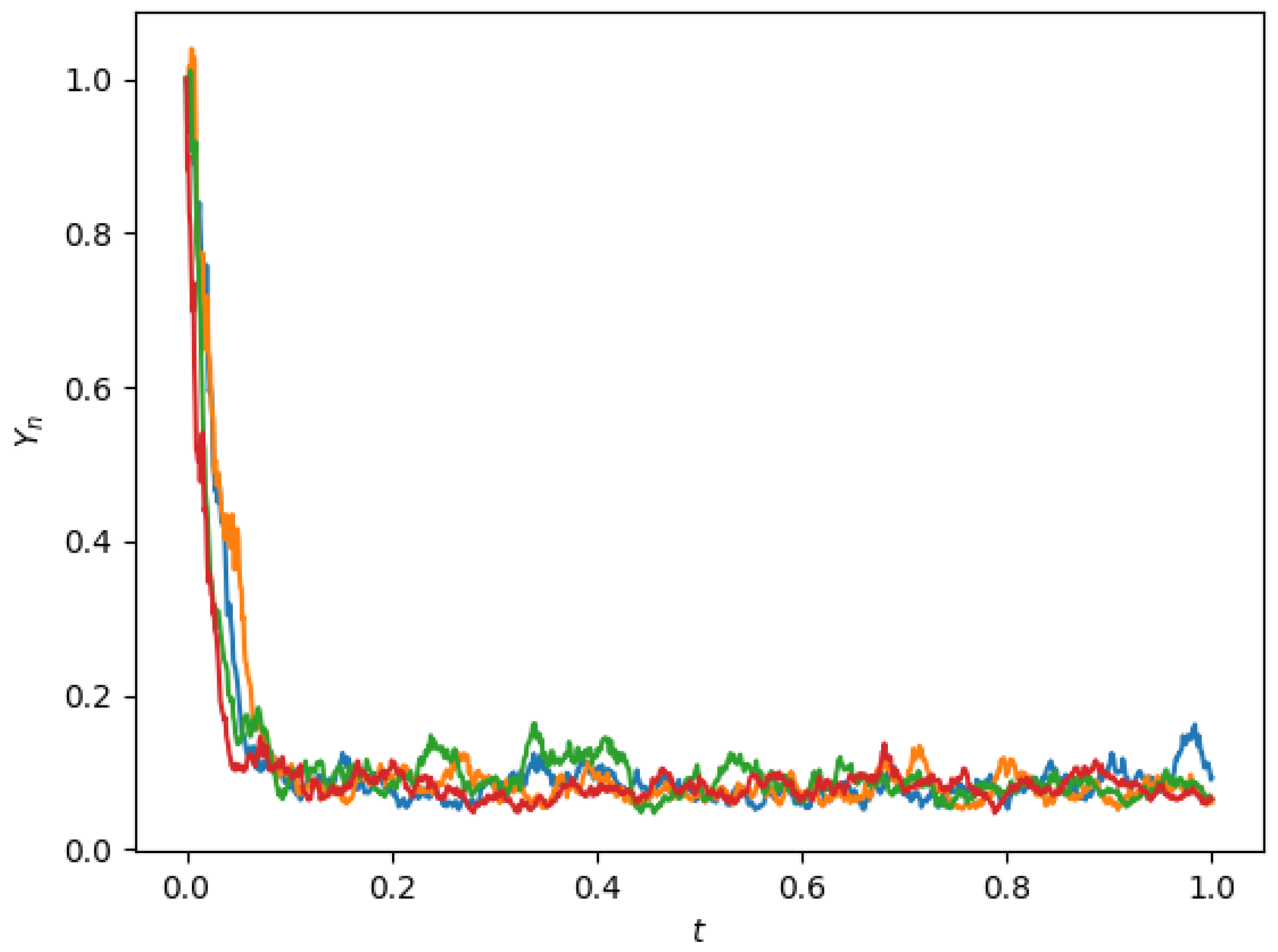
Therefore, inequality (24) is satisfied with ${\delta }_1=16$, ${\delta }_3=3/2$, ${\delta }_2=0$, ${\delta }_4=0.5$, and $k_3=0.1e^2$. By Lemma 4, the solution of (67) possesses the property of almost sure polynomial stability. Then, we select $\Gamma \left(b\right)=b^5$ and $\epsilon (\Delta )={\Delta }^{-1/4}$ to define the numerical solution of Equation (67) by using the partially truncated split-step theta (PTSS$\theta$) method (8). Moreover, the conditions of Theorem 3 are satisfied. Therefore the partially truncated split-step theta method applied to Equation (67) has almost sure polynomial stability when selecting $\theta \in (1/2,1]$. Figure 3 displays several trajectories of the partially truncated split-step theta (PTSS$\theta$) solutions (67), and it is clear that the numerical approximations have almost sure polynomial stability.

Figure 3. Trajectories of the partially truncated split-step theta (PTSS$\theta$) solutions for Equation (67), with $\theta =0.6$ and $\Delta =0.7$.

6. Conclusions

In this paper, the stochastic pantograph model with Lévy jumps is presented and the partially truncated split-step theta method is applied to it. The finite time ${\mathcal{L}}^{\widehat{\varrho }}(\widehat{\varrho }\ge 2)$ convergence rate was obtained, under both drift and diffusion coefficients, satisfying the super-linear growth condition while the jump coefficient grows linearly, and it was close to half. By setting theta equal to zero, the proposed scheme can be viewed as the partially truncated Euler–Maruyama method, which indicates that our results are more general. By utilizing the discrete semi-martingale convergence theorem, the numerical scheme reproduced the almost sure polynomial stability of the exact solution. The conditions imposed on the numerical scheme to reproduce the almost sure polynomial stability were sufficient, but not necessary. Therefore, our future work will focus on finding out the sufficient and necessary conditions. Other interesting topics would be to study the convergence rate with all coefficients growing super-linearly and trying to improve the convergence order of the proposed scheme.

References

- Meng, X.; Hu, S.; Wu, P. Pathwise estimation of stochastic differential equations with unbounded delay and its application to stochastic pantograph equations. Acta Appl. Math. 2011, 113, 231–246. [Google Scholar] [CrossRef]
- Ockendon, J.R.; Tayler, A.B. The dynamics of a current collection system for an electric locomotive. Proc. R. Soc. Lond. A Math. Phys. Sci. 1971, 322, 447–468. [Google Scholar]
- Kou, S.G. A jump-diffusion model for option pricing. Manag. Sci. 2002, 48, 1086–1101. [Google Scholar] [CrossRef]
- Svishchuk, A.; Kalemanova, A. The stochastic stability of interest rates with jump changes. Theory Probab. Math. Stat. 2000, 61, 161–172. [Google Scholar]
- Merton, R.C. Option pricing when underlying stock returns are discontinuous. J. Financ. Econ. 1976, 3, 125–144. [Google Scholar] [CrossRef]
- Black, F.; Scholes, M. The pricing of options and corporate liabilities. J. Political Econ. 1973, 81, 637–654. [Google Scholar] [CrossRef]
- Li, G.; Yang, Q. Stability analysis of the θ-method for hybrid neutral stochastic functional differential equations with jumps. Chaos Solitons Fractals 2021, 150, 111062. [Google Scholar] [CrossRef]
- Hobson, D.G.; Rogers, L.C. Complete models with stochastic volatility. Math. Financ. 1998, 8, 27–48. [Google Scholar] [CrossRef]
- Arriojas, M.; Hu, Y.; Mohammed, S.E.; Pap, G. A delayed Black and Scholes formula. Stoch. Anal. Appl. 2007, 25, 471–492. [Google Scholar] [CrossRef]
- Tankov, P. Financial Modelling with Jump Processes; Chapman and Hall/CRC: Boca Raton, FL, USA, 2003. [Google Scholar]
- He, L.; Banihashemi, S.; Jafari, H.; Babaei, A. Numerical treatment of a fractional order system of nonlinear stochastic delay differential equations using a computational scheme. Chaos Solitons Fractals 2021, 149, 111018. [Google Scholar] [CrossRef]
- Haghighi, A.; Rößler, A. Split-step double balanced approximation methods for stiff stochastic differential equations. Int. J. Comput. Math. 2019, 96, 1030–1047. [Google Scholar] [CrossRef]
- Geng, Y.; Song, M.; Liu, M. The convergence of truncated Euler-Maruyama method for stochastic differential equations with piecewise continuous arguments under generalized one-sided Lipschitz condition. J. Comput. Math. 2023, 41, 647–666. [Google Scholar] [CrossRef]
- Mao, X. Convergence rates of the truncated Euler–Maruyama method for stochastic differential equations. J. Comput. Appl. Math. 2016, 296, 362–375. [Google Scholar] [CrossRef]
- Huang, C. Mean square stability and dissipativity of two classes of theta methods for systems of stochastic delay differential equations. J. Comput. Appl. Math. 2014, 259, 77–86. [Google Scholar] [CrossRef]
- Liu, L.; Mo, H.; Deng, F. Split-step theta method for stochastic delay integro-differential equations with mean square exponential stability. Appl. Math. Comput. 2019, 353, 320–328. [Google Scholar] [CrossRef]
- Liu, L.; Deng, F.; Qu, B.; Fang, J. Stability analysis of split-step theta method for neutral stochastic delayed neural networks. J. Comput. Appl. Math. 2022, 417, 114536. [Google Scholar] [CrossRef]
- Rathinasamy, A.; Mayavel, P. The balanced split step theta approximations of stochastic neutral Hopfield neural networks with time delay and Poisson jumps. Appl. Math. Comput. 2023, 455, 128129. [Google Scholar] [CrossRef]
- Yang, X.; Yang, Z.; Zhang, C. Numerical Analysis of Split-Step Backward Euler Method with Truncated Wiener Process for a Stochastic Susceptible-Infected-Susceptible Model. J. Comput. Biol. J. Comput. Mol. Cell Biol. 2023, 30, 1098–1111. [Google Scholar] [CrossRef]
- Wu, D.; Li, Z.; Xu, L.; Peng, C. Mean square stability of the split-step theta method for non-linear time-changed stochastic differential equations. Appl. Anal. 2023, 103, 1733–1750. [Google Scholar] [CrossRef]
- Wu, X.; Gan, S. Convergence Rates of Split-Step Theta Methods for SDEs with Non-Globally Lipschitz Diffusion Coefficients. East Asian J. Appl. Math. 2023, 180, 16–32. [Google Scholar] [CrossRef]
- Higham, D.J.; Mao, X.; Stuart, A.M. Strong convergence of Euler-type methods for nonlinear stochastic differential equations. SIAM J. Numer. Anal. 2002, 40, 1041–1063. [Google Scholar] [CrossRef]
- Wang, P.; Liu, Z. Split-step backward balanced Milstein methods for stiff stochastic systems. Appl. Numer. Math. 2009, 59, 1198–1213. [Google Scholar] [CrossRef]
- Wang, P.; Li, Y. Split-step forward methods for stochastic differential equations. J. Comput. Appl. Math. 2010, 233, 2641–2651. [Google Scholar] [CrossRef]
- Liu, L.; Zhu, Q. Mean square stability of two classes of theta method for neutral stochastic differential delay equations. J. Comput. Appl. Math. 2016, 305, 55–67. [Google Scholar] [CrossRef]
- Wang, X.; Gan, S. The improved split-step backward Euler method for stochastic differential delay equations. Int. J. Comput. Math. 2011, 88, 2359–2378. [Google Scholar] [CrossRef]
- Zong, X.; Wu, F.; Huang, C. Exponential mean square stability of the theta approximations for neutral stochastic differential delay equations. J. Comput. Appl. Math. 2015, 286, 172–185. [Google Scholar] [CrossRef]
- Zhang, H.; Gan, S.; Hu, L. The split-step backward Euler method for linear stochastic delay differential equations. J. Comput. Appl. Math. 2009, 225, 558–568. [Google Scholar] [CrossRef]
- Cao, W.; Hao, P.; Zhang, Z. Split-step θ-method for stochastic delay differential equations. Appl. Numer. Math. 2014, 76, 19–33. [Google Scholar] [CrossRef]
- Bao, X.; Hu, L. Convergence and stability of split-step θ methods for stochastic variable delay differential equations. Int. J. Comput. Math. 2023, 100, 1171–1192. [Google Scholar] [CrossRef]
- Voss, D.A.; Khaliq, A.Q.M. Split-step Adams–Moulton Milstein methods for systems of stiff stochastic differential equations. Int. J. Comput. Math. 2015, 92, 995–1011. [Google Scholar] [CrossRef]
- Buckwar, E.; Winkler, R. Multi-Step Maruyama Methods for Stochastic Delay Differential Equations. Stoch. Anal. Appl. 2007, 25, 933–959. [Google Scholar] [CrossRef]
- Lu, Y.; Zhang, H.; Hong, S. Convergence and stability of the split-step composite theta-Milstein method for stochastic delay differential equations. Int. J. Dyn. Control 2023, 12, 1302–1313. [Google Scholar] [CrossRef]
- Zhang, Y.; Zhang, E.; Li, L. The Improved Stability Analysis of Numerical Method for Stochastic Delay Differential Equations. Mathematics 2022, 10, 3366. [Google Scholar] [CrossRef]
- Guo, Q.; Liu, W.; Mao, X.; Yue, R. The partially truncated Euler–Maruyama method and its stability and boundedness. Appl. Numer. Math. 2017, 115, 235–251. [Google Scholar] [CrossRef]
- Mao, W.; Hu, L.; Mao, X. The existence and asymptotic estimations of solutions to stochastic pantograph equations with diffusion and Lévy jumps. Appl. Math. Comput. 2015, 268, 883–896. [Google Scholar] [CrossRef]
- Nane, E.; Ni, Y. Stability of stochastic differential equation driven by time-changed L∖’evy noise. arXiv 2016, arXiv:1604.07382. [Google Scholar]
- Haghighi, A. A modified split-step truncated Euler-Maruyama method for SDEs with non-globally Lipschitz continuous coefficients. Comput. Methods Differ. Equ. 2023, 11, 522–534. [Google Scholar]
- Zhan, W.; Gao, Y.; Guo, Q.; Yao, X. The partially truncated Euler–Maruyama method for nonlinear pantograph stochastic differential equations. Appl. Math. Comput. 2019, 346, 109–126. [Google Scholar] [CrossRef]
- Abou-Senna, A.; AlNemer, G.; Zhou, Y.; Tian, B. Convergence Rate of the Diffused Split-Step Truncated Euler–Maruyama Method for Stochastic Pantograph Models with Lévy Leaps. Fractal Fract. 2023, 7, 861. [Google Scholar] [CrossRef]
- Zhang, T.; Gao, C. Stability with general decay rate of hybrid neutral stochastic pantograph differential equations driven by Lévy noise. Discret. Contin. Dyn. Syst. B 2022, 27, 3725–3747. [Google Scholar] [CrossRef]
- Guo, P.; Li, C.J. Almost sure exponential stability of numerical solutions for stochastic pantograph differential equations. J. Math. Anal. Appl. 2018, 460, 411–424. [Google Scholar] [CrossRef]
- Mao, X.; Yuan, C. Stochastic Differential Equations with Markovian Switching; Imperial College Press: London, UK, 2006; pp. 77–110. [Google Scholar]
- Song, M.; Lu, Y.; Liu, M. Convergence of the tamed Euler method for stochastic differential equations with piecewise continuous arguments under non-global Lipschitz continuous coefficients. Numer. Funct. Anal. Optim. 2018, 39, 517–536. [Google Scholar] [CrossRef]
- Tan, J.; Wang, H. Convergence and stability of the split-step backward Euler method for linear stochastic delay integro-differential equations. Math. Comput. Model. 2010, 51, 504–515. [Google Scholar] [CrossRef]
Disclaimer/Publisher’s Note: The statements, opinions and data contained in all publications are solely those of the individual author(s) and contributor(s) and not of MDPI and/or the editor(s). MDPI and/or the editor(s) disclaim responsibility for any injury to people or property resulting from any ideas, methods, instructions or products referred to in the content. |
© 2024 by the authors. Licensee MDPI, Basel, Switzerland. This article is an open access article distributed under the terms and conditions of the Creative Commons Attribution (CC BY) license (https://creativecommons.org/licenses/by/4.0/).