A Rapid Detection Method for Coal Ash Content in Tailings Suspension Based on Absorption Spectra and Deep Feature Extraction

Abstract

Traditional visual detection methods that employ image data are often unstable due to environmental influences like lighting conditions. However, microfiber spectrometers are capable of capturing the specific wavelength characteristics of tail coal suspensions, effectively circumventing the instability caused by lighting variations. Utilizing spectral analysis techniques for detecting ash content in tail coal appears promising as a more stable method of indirect ash detection. In this context, this paper proposes a rapid detection method for the coal ash content in tailings suspensions based on absorption spectra and deep feature extraction. Initially, a preprocessing method, the inverse time weight function (ITWF), is presented, focusing on the intrinsic connection between the sedimentation phenomena of samples. This enables the model to learn and retain spectral time memory features, thereby enhancing its analytical capabilities. To better capture the spectral characteristics of tail coal suspensions, we designed the DSFN (DeepSpectraFusionNet) model. This model has an MSCR (multi-scale convolutional residual) module, addressing the conventional models’ oversight of the strong correlation between adjacent wavelengths in the spectrum. This facilitates the extraction of relative positional information. Additionally, to uncover potential temporal relationships in sedimentation, we propose a CLSM-CS (convolutional long-short memory with candidate states) module, designed to strengthen the capturing of local information and sequential memory. Ultimately, the method employs a fused convolutional deep classifier to integrate and reconstruct both temporal memory and positional features. This results in a model that effectively correlates the ash content of suspensions with their absorption spectral characteristics. Experimental results confirmed that the proposed model achieved an accuracy of 80.65%, an F1-score of 80.45%, a precision of 83.43%, and a recall of 80.65%. These results outperformed recent coal recognition models and classical temporal models, meeting the high standards required for industrial on-site ash detection tasks.

1. Introduction

Industrial coal slurry flotation is a widely employed physical separation technique for processing various coal waste materials, such as coal gangue and coal slurry. As shown in Figure 1, the primary aim of this method is to enhance the grade of coal (its coal content) and minimize waste by separating coal particles from other impurities in the coal slurry through bubble adsorption. The real-time monitoring of key performance indicators during the production process has increasingly become a focal point of interest in both industrial and academic circles. This heightened attention aims to augment the efficiency of coal slurry flotation technology.

Figure 1. Slime flotation process flow.

Reagents, flotation concentration, and air inflow influence the quality of coal slurry flotation [1]. Ash content in the tailings is an important indicator for assessing the quality of floated coal and serves as a crucial basis for the rational application of flotation coal. If the ash content in the tailings is low, this indicates that the flotation process has effectively separated impurities and ash components from coal particles, thereby improving the coal’s grade. This usually means that the flotation technology is efficient and the coal quality is better, leading to a higher value in subsequent industrial applications. Conversely, a high tailings ash content indicates poor separation in the flotation process, where impurities and ash components are inadequately separated from coal particles. This may be due to poor bubble adsorption, improper use of chemical reagents, or insufficient bubble generation, among other reasons. A high tailings ash content can reduce the coal’s grade and, consequently, lower its industrial usability.

Traditional methods for ash content detection in coal slurry flotation mainly include radiation measurement and image processing. The radiation measurement method uses the attenuation of X-rays in coal to measure the content of high atomic number elements in coal, from which ash content can be estimated. This non-contact method is suitable for online detection in special environments such as high temperature and pressure. However, it involves using radioactive sources and carries certain safety risks. On the other hand, image processing uses machine vision techniques to extract image features from the surface of coal or foam layers. Then, it establishes a relationship model between image features and ash content to estimate the ash content. This method can capture information about coal particle shapes, colors, and other features to a certain extent through machine learning, providing more potential information. However, it can only measure the surface ash content of flotation and cannot reflect the distribution of internal ash content. Moreover, environmental lighting conditions severely affect the image quality and detection accuracy, requiring appropriate calibration and control.

Therefore, we compiled a comparison of the advantages and disadvantages of the main research objects currently in use, as shown in Table 1. Currently, the detection of ash content in coal slurry flotation tailings typically involves collecting images of dried coal powder or flotation froth as datasets. However, these methods all share the limitation of being heavily influenced by the quality of the images, which is significantly affected by environmental lighting conditions. It is difficult to rigorously control lighting factors in industrial environments. As for the reflectance spectra, they are sampled based on the reflective properties of substances to light. However, fundamentally, they still use dried coal powder as the research object, which has the following drawbacks: Firstly, during the coal slurry flotation process, tail coal is usually in a suspended state. To obtain dried coal powder, drying is required, which takes tens of minutes to several hours to complete, not meeting industrial requirements and entailing significant delays. Secondly, the above methods can only obtain surface information of samples and cannot reflect deep internal information. To address these issues, we considered using absorption spectra of tailings suspension as the research object. The benefits of this approach are as follows: Firstly, it directly eliminates the drying step, greatly shortening the detection time and meeting rapid industrial requirements. Secondly, absorption spectra can reflect the dynamic changes in suspended liquid samples, containing rich feature information. To address the difficulty of capturing these features, we considered using deep learning methods to fully explore deep information, relying on its powerful modeling capabilities. In summary, this paper proposes a rapid detection method for coal ash content in tailings suspensions based on absorption spectra and deep feature extraction. The spectral data of tail coal suspensions were preprocessed using the inverse time weight preprocessing method. The DSFN model was designed to extract location and time information from the spectral data using an MSCR module and CLSM-CS module. Finally, the features extracted by the two modules were fused and reconstructed to output information, thereby constructing a correlation model between the ash content of the suspension and the absorption spectral characteristics. The contributions of this paper are as follows:

Table 1. Comparison of different research objects for coal slime flotation ash content detection methods.

Research Object Type	Image Data		Spectral Data
	Coal Powder Solid Image	Coal Slurry Flotation Foam Image	Reflectance Spectrum	Absorption Spectrum
Advantages	Visually observes sample manifestation	Reflects foam status during flotation process	Provides surface composition details	Real-time monitoring Dynamic sample capture
Limitations	Large detection lag Affected by coal particle size and shape	Experimental conditions greatly affect foam morphology	Large detection lag Surface information lacks depth for detailed analysis	Random particle motion complicates feature capture
Common points	Its quality is greatly affected by lighting factors		Less susceptible to external interference

• Our method focuses on the absorption spectrum of tailings suspensions, marking the first study in the field to detect ash content in coal slurry flotation tailings. This approach not only meets the demands for industrial rapidity but also provides more comprehensive data.
• Traditional sequential preprocessing methods fail to effectively capture the temporal relationships inherent in the settling phenomena of tailings suspension samples. To address this, we propose an inverse time weight function (ITWF) that emphasizes differences at earlier time points, while still considering information from later time points.
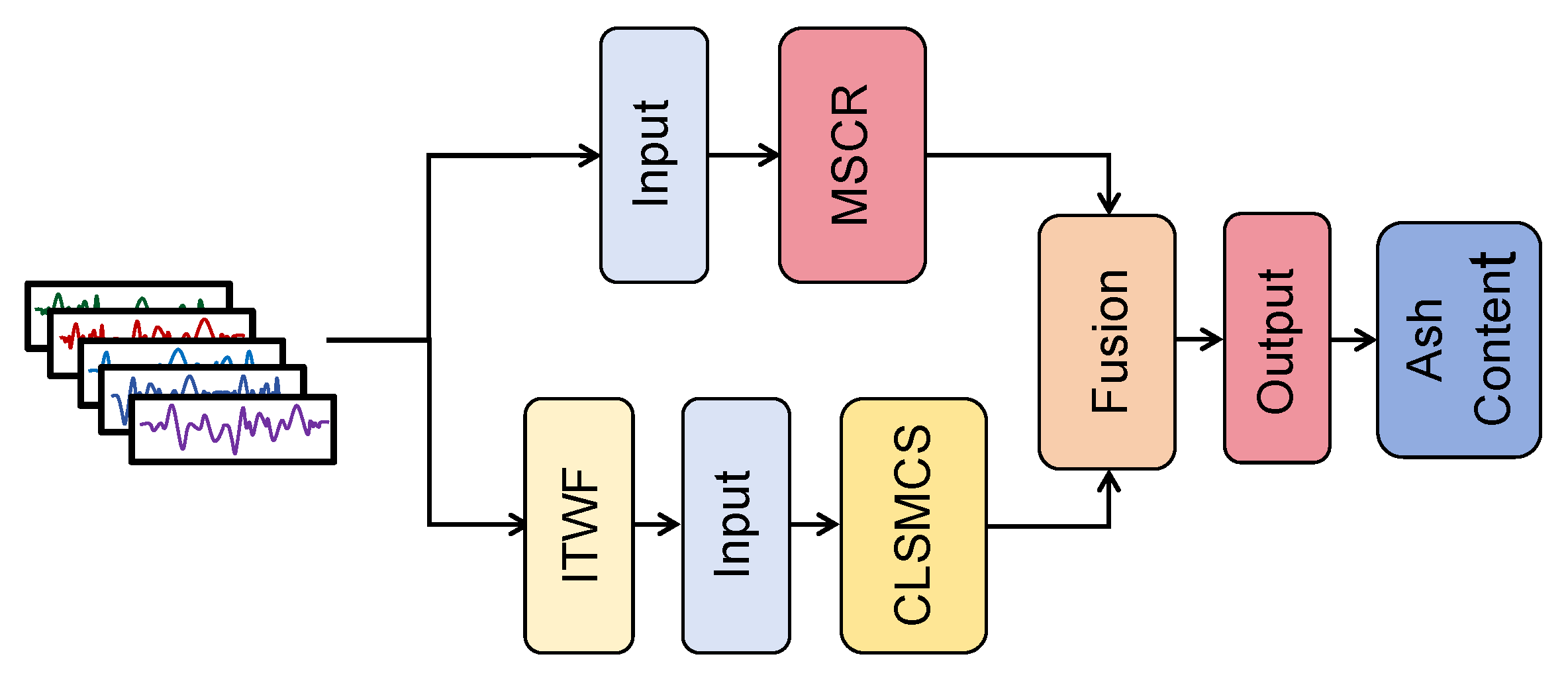
• Considering the unique characteristics of the absorption spectrum of tailings suspension, we designed the DSFN (DeepSpectraFusionNet) model. This model effectively captures the location-dependent features and time memory features of the tailings suspension absorption spectrum, yielding promising results.

2. Related Work

2.1. Radiation Method

Since the end of the last century, with the rapid development of civilian nuclear technology and computer technology, many rapid ash measurement techniques based on radiation methods have been proposed [2,3,4]. Radiation measurement methods utilize the attenuation pattern of the rays within coal to measure the content of high atomic number elements in coal, thereby estimating the ash content. Representative radiation-based ash measurement methods include low-energy gamma-ray backscattering [5], dual-energy gamma-ray transmission, and natural gamma radioactivity-based coal ash measurements [6]. Although these methods achieve rapid monitoring of ash content with good synchronization, the corresponding instrumentation is complex, maintenance and operational costs are high, and they require radioactive sources, posing radiation safety concerns.

2.2. Image Method

2.2.1. Image Method Based on Machine Learning

With improved computer hardware performance and the development of image processing algorithms, data-driven machine learning techniques have gradually been applied to coal ash content detection. Machine learning methods no longer require detailed prior knowledge; they only need to extract feature information from large datasets and construct correlation models between image features and ash content to achieve rapid real-time prediction of ash content in flotation tailings. Due to their non-contact nature, safety, flexibility, speed, and low cost advantages, data-driven ash content detection methods in flotation tailings have become a hot topic in current research. In this context, Gui Weihua and others made progress in key feature extraction and characterization of foam images based on machine vision, rapid detection of key parameters, and automatic classification and recognition of operating conditions. They discussed implementing a foam image processing system based on machine vision [7]. Zhao and others used 70 different machine learning (ML) models to simulate the migration behavior of minerals during coal slurry flotation based on particle characteristics (shape, size, composition, and type). The results indicated that particle size and composition played the most significant role in coal slurry flotation [8]. Tan Liping and others reviewed recent advances in mineral flotation monitoring technology based on machine vision, including foam image segmentation techniques, extraction of visual features from flotation foam, dimensionality reduction, and flotation condition recognition strategies. They reported the current application status of foam flotation monitoring systems and, based on the characteristics of mineral flotation foam images, pointed out the new challenges foam monitoring technology faces [9]. Wang Jingqian and others collected colored tailings images and used color features and other information as input variables. They employed the particle swarm optimization algorithm to predict ash content using the LSSVM model, improving prediction accuracy [10]. Ding Jianjun and others collected foam images from the first and third slots of a flotation machine, and extracted features such as bubble color, bubble collapse degree, bubble size and shape, and bubble movement speed. They established an ash content prediction model using support vector regression. Their results showed that the absolute error between the predicted and actual ash content was 0.34% and 0.37% for the first and third slots, respectively [11].

2.2.2. Image Method Based on Deep Learning

Although these models have made significant progress, there are still some unresolved issues and room for improvement. Firstly, most of these models are shallow learning models with limited expressive and generalization capabilities. They cannot fully explore the corresponding latent information and struggle to provide a deep-level and rapid description of image data with ash content indicators. Secondly, traditional computer vision methods often require manual designing of feature extraction algorithms, which may require domain experts and often yields subpar results when dealing with complex scenes. Deep learning can address the two main challenges faced in real-time rapid detection of tailings ash content. Firstly, the multi-layer network structure in deep learning allows models to learn feature representations layer by layer. This hierarchical feature learning can extract information at different levels of abstraction from the data, thus better capturing the intrinsic structure of the data. Secondly, deep learning models can achieve end-to-end learning, automatically learning higher-level, richer feature representations from raw data through the structure of multi-layer neural networks, reducing the burden of feature engineering. Guo Xijin and others extracted features from tailings ash content images using a multi-layer neural network, then regressed the tailings ash content values and compared them with actual tailings ash content values. Experimental results showed that their coal slurry flotation tailings ash content detection based on deep convolutional networks had good real-time performance, and the detection accuracy met production requirements [12]. Wen and others trained several advanced convolutional neural networks on an augmented coal flotation foam image dataset. The results showed that abstract pixel features were significantly superior to manually designed features [13]. Yang and others proposed a new hybrid model, a convolution–attention parallel network (CAPNet), which quickly and accurately determined the ash content of a coal flotation concentrate by analyzing foam images. The results indicated that CAPNet outperformed other methods such as CNN regarding accuracy and stability [14]. Han Yu and others constructed a CNN-BP composite model, leveraging the strengths of both CNN and BP for tailings ash content prediction, achieving good model accuracy and meeting production requirements [15]. These achievements demonstrate that deep learning has achieved excellent predictive performance when applied to the problem of flotation ash content detection, exhibiting strong industrial applicability.

2.3. Spectral Analysis

It is worth noting that current tailings ash content detection methods using deep learning models focus on tailings images as the research object. The main drawback of image-based methods is that lighting conditions heavily influence the quality of image data collected in industrial settings. Industrial environments often do not consider lighting factors in coal slurry flotation, and they do not typically provide stable lighting conditions. As a result, the effectiveness of deep learning combined with image processing methods is greatly constrained by this limitation. Therefore, there is an urgent need to develop a more stable and simultaneously high-accuracy and rapid tailings ash content detection method.

Changing the approach to spectral analysis is a suitable method of ash content detection [16]. Firstly, spectrometers have a low dependence on environmental conditions when analyzing materials. For example, spectrometers can operate stably under different lighting conditions. At the same time, the performance of machine vision systems may be significantly affected by changes in lighting (e.g., cloudy days, direct sunlight, etc.). Secondly, spectrometers identify and classify substances by analyzing their spectral characteristics, which is a direct method of analyzing material properties. In contrast, machine vision relies on image features such as color, shape, texture, etc., which may change due to external factors such as dust, moisture, lighting, etc. Additionally, miniaturized fiber-optic spectrometers offer portability, speed, non-destructiveness, etc., making them well-suited for industrial on-site testing requirements. Spectral analysis is a relatively novel method that meets the abovementioned requirements for tailings ash content detection.

With the advancement of miniaturized spectrometers and their spectral analysis technologies, applying spectral analysis in material analysis and sample testing has gained increasing attention. Researchers have begun to explore the combination of spectral analysis and deep learning methods in various domains. For example, Yang et al. developed a series of convolutional neural networks (CNNs) based on near-infrared spectroscopy for various tea data classification tasks [17]. Yu et al. used near-infrared spectroscopy of ground coffee as input to predict the flavor of premium coffee, investigating the feasibility of training machine learning and deep learning models, providing a new objective framework for predicting the complex flavors of food and beverage products [18]. Li et al. proposed spectral technology for soil classification, replacing remote sensing image information with spectral information. They used deep learning models to establish soil models of different types, achieving rapid and non-destructive soil classification [19]. Xiao et al. collected spectral information of SAS samples using a visible-near-infrared spectrometer and developed models based on convolutional neural networks, a gravity search algorithm, and an extreme learning machine to achieve rapid detection of salt content [20]. Liu et al. proposed a predictive model using near-infrared spectroscopy and deep learning for the rapid and accurate non-destructive detection of artificial bright blue pigments in ice cream [21]. Bai et al. evaluated the modeling and prediction capabilities of various machine learning techniques using near-infrared spectroscopy data from 118 instant tea samples, confirming the applicability of machine learning for optimizing models of instant tea composition detection based on near-infrared methods [22]. Ravichandran et al. innovatively suggested using a convolutional neural network based on near-infrared spectroscopy, instead of wet chemistry and image processing methods, for the early-stage screening of rice breeding programs [23]. Lee et al. proposed a method that combines spectral clustering techniques with support vector machines (SVM) to recognize control chart patterns (CCPs) under a gamma distribution. This method generally outperformed the Shewhart chart and EWMA chart with run rules in terms of recognition efficiency, which was demonstrated through a real-world case study of the tire manufacturing process [24]. Ma et al. proposed a multi-scale spatial–spectral transformer (MSST), which effectively captures global dependencies and spatial–spectral information in hyperspectral images (HSI) through a spatial–spectral token generator (SSTG) and a token fusion self-attention (TFSA) module, achieving higher classification accuracy on three public datasets compared to state-of-the-art methods. These studies highlighted the superiority of deep learning methods and demonstrated the feasibility of combining spectral analysis technology with deep learning methods [25]. This approach holds promise for improving the accuracy and efficiency of ash content detection in tailings and other applications.

Xiao’s team has significantly contributed to applying spectral analysis in coal detection. Over the years, they have conducted extensive research using spectral analysis techniques. In 2018, they used a spectrometer to measure spectral data from different coal samples in China. They then extracted spectral features using convolutional neural networks (CNN) and constructed predictive analysis models for spectral feature data using extreme learning machine (ELM) algorithms. The results showed that the developed models could predict the composition of coal [26]. In 2019, they proposed an improved multi-layer ELM algorithm to establish a coal type classification model. Simulation results demonstrated that this model had a good classification performance [27]. In 2020, they used an SVC HR-1024 spectrometer to obtain visible-near-infrared spectral data from coal samples. They then constructed characteristic analysis models for coal using deep belief networks and two-layer ELM algorithms. This effectively predicted the coal’s components [28]. In 2021, they developed a coal identification model that combined convolutional neural networks and ELM. They optimized model parameters using the whale optimization algorithm. Experimental results showed that this method could rapidly and accurately identify coal types [29]. In 2022, they proposed the DR_TELM model, which extracted effective features from coal spectral data using convolutional neural networks (CNN), utilizing TELM as a regressor for feature recognition and content prediction. Experimental results indicated that DR_TELM achieved a high precision in predicting moisture, ash content, volatile matter, and ash content, while reducing the testing time [30]. In 2023, they proposed an identification method called IAT-TELM that combined machine learning with reflectance spectroscopy for identifying lignite, bituminous coal, and anthracite. Experimental results demonstrated that the IAT-TELM model exhibited the best performance and the highest classification accuracy among the compared algorithms. These research efforts highlighted the successful integration of spectral analysis and machine learning techniques for various aspects of coal analysis and classification, showcasing the potential for accurate and efficient coal characterization [31].

However, the research mentioned above on coal ash content detection faces two main challenges: Firstly, coal exists as a solid–liquid mixture (suspension) during the coal slurry flotation process. Current spectral analysis research primarily focuses on thoroughly dried coal powder solids as research objects, measuring their reflectance spectra as the dataset. Sampling, drying, and detection are still required during coal slurry flotation, which takes considerable time and causes significant delays. This does not fully meet the requirements of rapid monitoring of coal ash content during flotation and the need for timely adjustments to industrial strategies. Secondly, most of the research employed shallow-depth deep learning models with limited feature extraction capabilities. These challenges must be addressed to develop a more efficient and timely method for monitoring coal ash content during the coal slurry flotation process.

Therefore, based on an in-depth study of coal slurry flotation ash content detection, this paper proposes a rapid detection method for tail coal ash content. We employ a miniature fiber-optic spectrometer to capture specific wavelength characteristics of the tail coal suspension, thus avoiding the data instability caused by changes in lighting conditions in traditional methods. The application of spectral analysis technology enhances the stability of this method in ash content detection. To further improve the efficiency and accuracy of the detection method, we propose the concept of an ITWF (inverse time weight function). This method helps identify the inherent connections during the sample settling process, enabling the model to more effectively learn the temporal variations in spectral data. We also designed the DSFN (DeepSpectraFusionNet) model. This model features an MSCR (multi-scale convolutional residual) module to extract more effective relative positional dependency information. Additionally, to uncover potential temporal relationships in sedimentation, we propose a CLSM-CS (convolutional long-short memory with candidate states) module to enhance the capture of local information and temporal memory. Finally, by integrating a convolutional deep classifier, the time-memory features and positional dependency features are combined to construct an ash content detection model that accurately reflects the correlation between the suspended solids’ ash content and absorption spectral features.

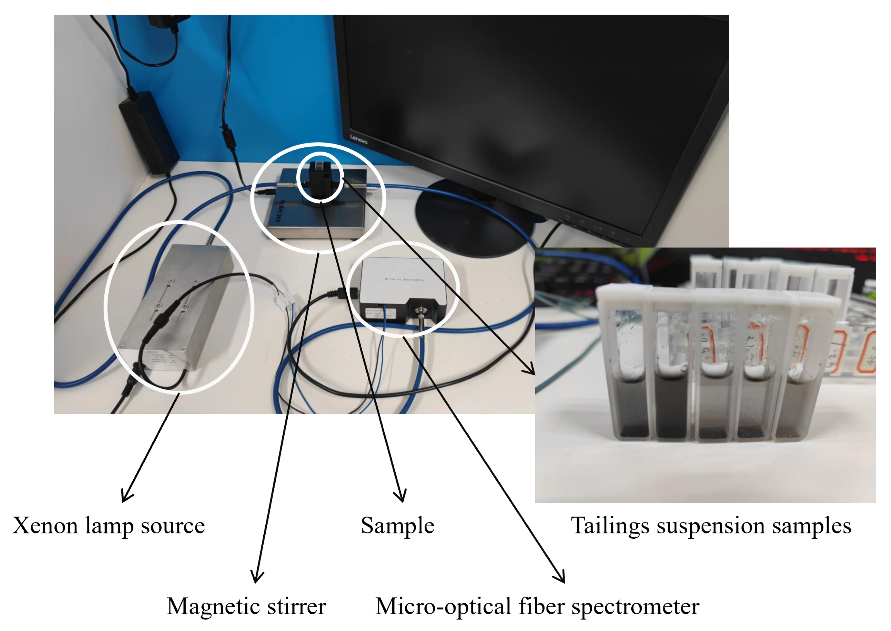
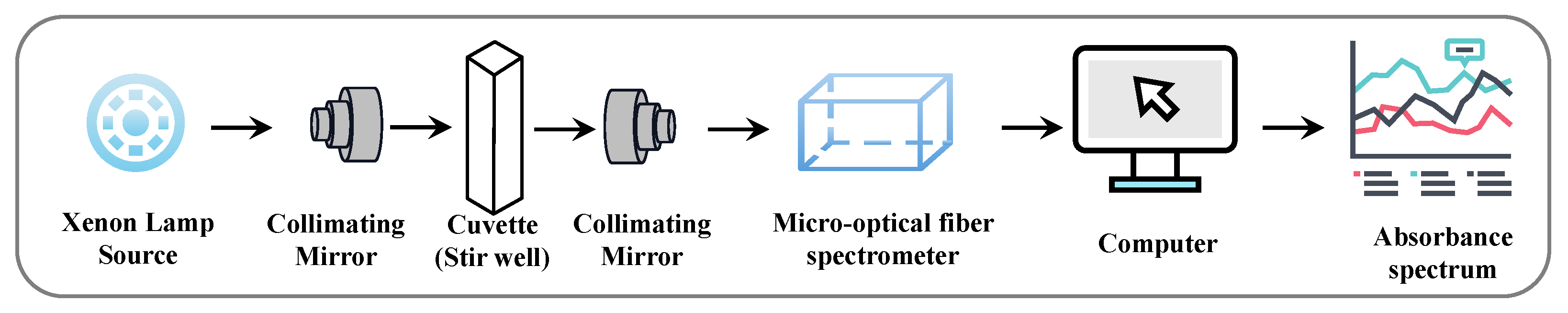
3. Materials and Methods

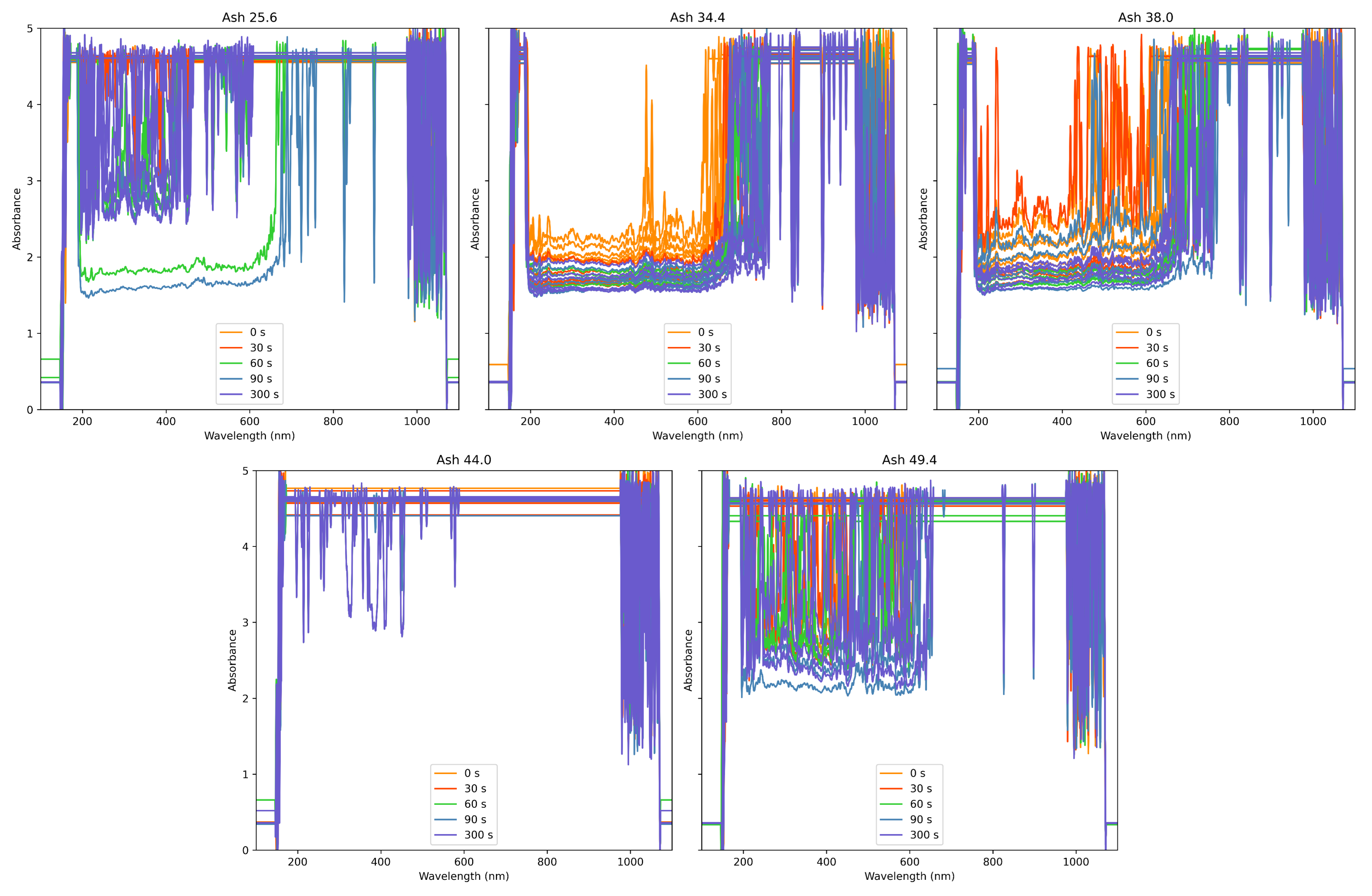
3.1. Data Description and Preprocessing

The experimental equipment required for building the data acquisition system using the absorption spectral data of tail coal suspensions included a quartz cuvette, a magnetic stirrer, a fiber-optic spectrometer, a UV quartz fiber optic, a dual-path cuvette holder, a pulsed xenon lamp light source, and so on. From Figure 2 and Figure 3, we can understand the data acquisition process. First, the xenon lamp light source instrument outputs light, which is then received by a collimating mirror and passes through a cuvette sample. Afterward, the light is output by another collimating mirror and received by a miniature fiber-optic spectrometer. The absorbance curve is displayed on the screen.

Figure 2. Experimental data collection site.

Figure 3. Spectrum acquisition flow chart.

The experimental samples consisted of tail coal samples with ash contents of 25.6%, 34.4%, 38.0%, 44.0%, and 49.4%. The corresponding ash content labels for these samples were accurately determined using the fast ashing experiment commonly employed in the industry. Each tail coal sample was mixed with an equal amount of pure water to create a suspension, simulating the state of tail coal extraction in an industrial setting. Samples were obtained by taking a portion of the suspension from each sample. Since the samples were in suspension, settling phenomena occurred over time. To mitigate the impact on the experimental results, we ran a magnetic stirrer for 5 min at the beginning of each experiment to ensure thorough mixing. The cuvette holder used had a hollow structure, allowing us to collect absorbance spectra immediately at 0 s after stopping the magnetic stirring. Then, the samples were allowed to settle, and the absorbance spectra were collected at 0 s, 30 s, 60 s, 90 s, and 300 s. For each category, 31 samples were taken at each time point, resulting in five ash content categories. Therefore, a total of 775 data samples were obtained. The data type is a one-dimensional univariate sequence containing 2088 feature points. Figure 4 shows spectral data curves for 30 randomly selected samples from each category. Each curve represents a spectral data sample, illustrating the general trend of the spectral data for each category.

Figure 4. Thirty randomly selected spectral data samples display.

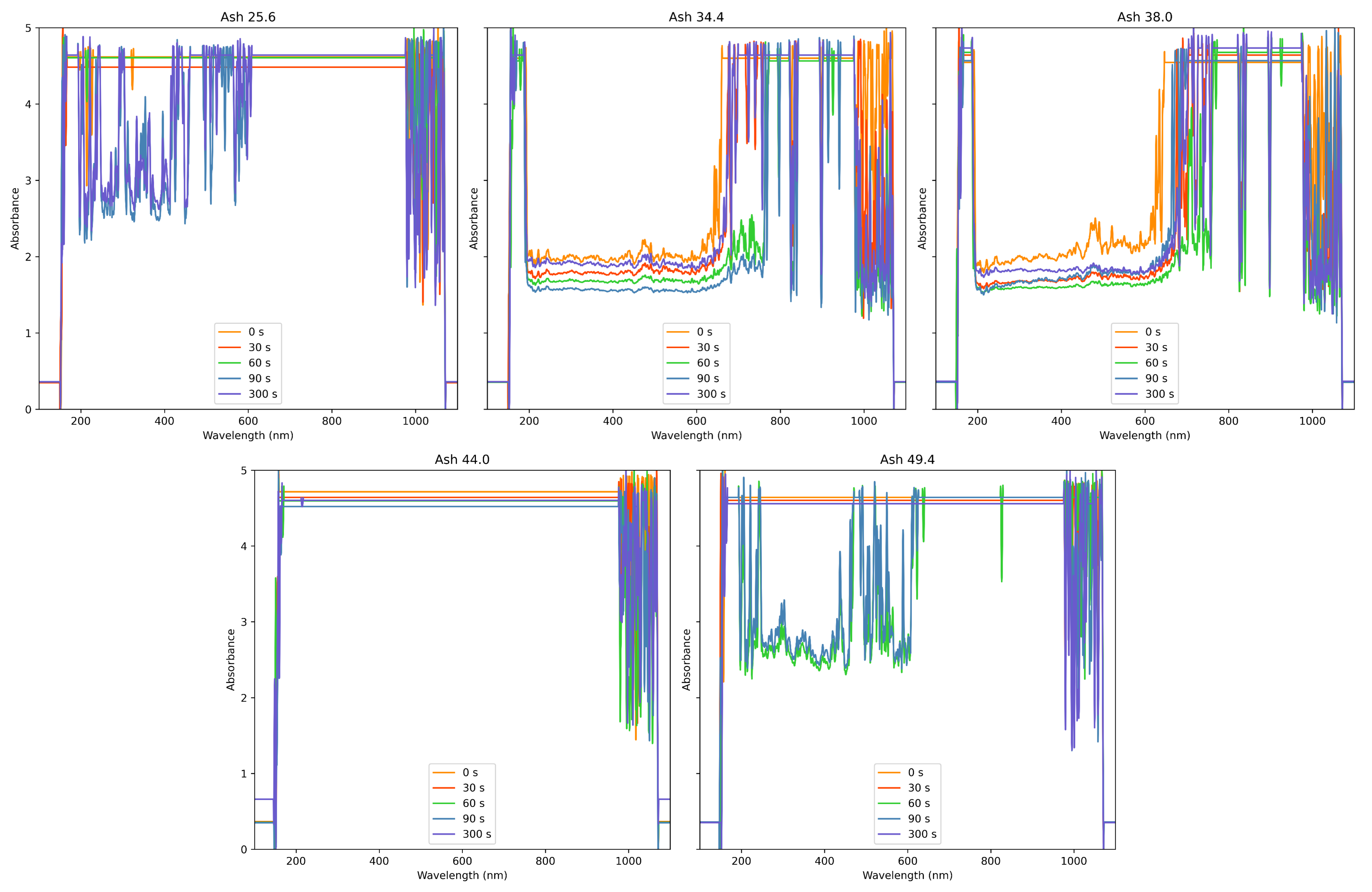
3.1.1. Data Preprocessing

Preprocessing is widely executed when analyzing spectral signals, to eliminate or reduce unnecessary variations in the original spectral data, such as noise bands and outliers. Moreover, appropriate preprocessing is crucial for enhancing the accuracy of neural networks [32].

Preprocessing included three steps. Firstly, second-order polynomial Savitzky–Golay (SG) smoothing denoised the input data’s raw absorbance spectra. Savitzky–Golay smoothing is a technique used to smooth data by fitting local data with a polynomial, which helps reduce noise and outliers, while preserving the data’s main features. Its formula is as follows:

$$Y_i=\sum _{j=-k}^k{c}_j·Y_{i+j}$$

(1)

where $Y_i$ represents the smoothed data, i indicates the index of the data points in the series, k is the order of the polynomial fitted, and $c_j$ are the Savitzky–Golay coefficients.

Secondly, first-order derivative correction was utilized to correct baseline drift. This step aimed to correct the baseline drift, which is the gradual increasing or decreasing trend that might exist in a spectrum. By calculating the data’s first-order derivative (difference), baseline drift can be eliminated, thereby better highlighting the absorption peaks in the spectrum. Its formula is as follows:

$$D_i=Y_{i+1}-Y_i$$

(2)

$$Y_i^{\prime }=Y_i-mean\left(D\right)$$

(3)

where $D_i$ is the first-order derivative of the original data, $Y_i^{\prime }$ is the corrected data point after baseline drift correction, and $mean\left(D\right)$ represents the mean value of the first-order derivative.

$$Z_i=\frac{Y_{i^{\prime }}-min\left(Y_{i^{\prime }}\right)}{max\left(Y_{i^{\prime }}\right)-min\left(Y_{i^{\prime }}\right)}$$

(4)

where $max\left(Y_{i^{\prime }}\right)$ and $min\left(Y_{i^{\prime }}\right)$ are the minimum and maximum values of the corrected data, respectively.

This benefits many machine learning algorithms by reducing the amplitude differences between different features, aiding the model in better convergence and prediction. The processed data are shown in Figure 4.

3.1.2. Inverse Time Weight Function

Beyond the usual spectrum preprocessing methods, the data analysis also had to account for the settling phenomenon of the suspended liquid samples. As illustrated in Figure 5, particles within the suspension generally possessed higher densities than the liquid medium, causing them to gradually settle or precipitate over time. Figure 6 showcases the evolution of the absorption spectra over different time intervals, displaying a discernible, orderly gradient-like transition from 0 to 300 s.

Figure 5. Sedimentation phenomenon of tail coal.

Figure 6. Changes in spectral data at different times.

Based on this, we proposed an inverse time weight function (ITWF). At moment 0, the sample data contain the richest information regarding differences. As time progresses, the coal tailings particles continually settle to the bottom and come to rest, making the absorption spectrum at this stage similar to that of pure water, containing the least amount of information. A weight decay factor emphasizes data from earlier time points, focusing on the differences at these points, while not ignoring information from later times. Data collection was performed at different time points for the same sample, and a temporal memory rule was used between the corresponding absorption spectra. These samples were further processed into temporal memory data, enabling the subsequent models to better mine temporal feature information. The specific formula is as follows:

$$Y_t=\frac{{\sum }_{i=1}^n{\alpha }^i{x}_{it}}{{\sum }_{i=1}^n{\alpha }^i}$$

(5)

where $x_i$ represents the absorption spectrum sequence at different time points, and ${\alpha }^i$ is the weight decay factor.

3.2. Model Framework

Building upon in-depth research into coal slime flotation ash content detection, this paper proposed a rapid detection method for coal ash content in tailings suspension based on absorption spectra and deep feature extraction. The overall framework of the DSFN is shown in Figure 7.

Figure 7. Overall framework structure.

Following the data collection and preprocessing methods described above, the data were processed into an original dataset and a temporary dataset. To address the distinct characteristics of these datasets, we designed an MSCR module and CLSM-CS module to extract specific features. After completing the information extraction for each module, a fused convolutional deep classifier was employed to merge and reconstruct the dual information. This approach enabled the construction of a model that correlated the ash content in the suspension with its absorption spectral characteristics for ash detection.

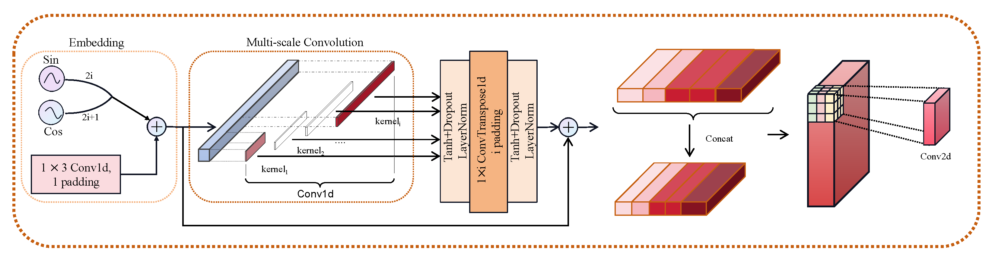
3.2.1. Multi-Scale Convolutional Residual Module

As shown in Figure 8 and Figure 9, we have used two types of figures to make the description of this module clearer. In the diagram, [1 × 3]:14 indicates a convolutional kernel size of 1 × 3 with 14 output channels, and so on. To address the differentiated features of spectral data at various wavelengths, this paper designed an MSCR module based on conventional convolutional neural networks. Traditional convolutional neural networks typically use fixed-size convolution kernels, which may result in a limited receptive field and difficulty in effectively capturing features of different scales and levels in the input data. Additionally, conventional convolution operations only extract information within a local receptive field, potentially making it difficult for the model to understand long-distance dependencies between pixels. By introducing convolution kernels of multiple scales, the model can better process features of different scales. Smaller kernels can capture finer details, while larger ones can capture broader contextual information. Conventional multi-scale convolutions usually just concatenate information of different scales, potentially overlooking the contextual relationships between scales and generating redundant information. To address these issues, residual connections and two-dimensional convolutional concatenation were introduced. Residual connections provide a direct shortcut bypassing intermediate layers, establishing long-distance information dependencies, allowing for faster information propagation and enabling the model to learn residual features and the differences between the input and output. Concatenating features of different scales and using two-dimensional convolution for feature extraction avoids redundancy, while reducing computational and memory overheads. The specific steps are as follows:

Figure 8. MSCR Module Visualization Flowchart.

Figure 9. MSCR Module Structure Diagram.

First, the data are processed with embedding, to convert the discrete wavelength data into continuous, dense vector representations. The formula is as follows:

$$PE=\left\{\begin{array}{c}p{e}_{pos,2i}=sin\frac{pos}{{10,000}^{\frac{2i}{d_{\mathrm{model}}}}}\hfill \\ p{e}_{\mathrm{pos},2i+1}=cos\frac{pos}{{10,000}^{\frac{2i}{d_{\mathrm{model}}}}}\hfill \end{array}\right.$$

(6)

$$VE=Conv1d\left(X_b\right)$$

(7)

$$X_{emb}=sum(VE+PE)$$

(8)

where $PE$ represents position embedding, $pos$ is the position in the input sequence, $d_{model}$ is the dimension of the model, $i\in (0,\frac{d_{model}}{2}-1)$, and $VE$ represents numerical embedding.

Then, a set of convolution kernels of different scales was designed to extract features from the data. This enables the model to more comprehensively understand time-series data and learn features and patterns at different window scales. The specific steps are as follows:

$$X_i=Norm\left(Dropout\left(Tanh\left(Conv1d{\left(x_{\mathrm{emb}}\right)}_{\mathrm{kernel}=\mathrm{i}}\right)\right)\right)$$

(9)

where i is the index of the convolution kernel, corresponding to different kernel sizes for convolution.

Then, upsampling and truncation operations are performed to match the sequence length for subsequent processing. The features extracted are added to the original output to form a residual connection, with the specific steps as follows:

$$Y_i=Truncate\left(Norm\left(Dropout\left(Tanh\left(ConvTranspose1d{\left(X_i\right)}_{\mathrm{kernel}=\mathrm{i}}\right)\right)\right)\right)$$

(10)

$$Z_i=X_{emb}+Y_i$$

(11)

After processing through the MSCR module, the feature representations processed under different sliding windows are stored in a list for subsequent processing. This list contains features at multiple scales, which are expanded by one dimension. The features of several scales are concatenated in the newly added dimension according to the number of multi-scale convolution kernels. The resulting new features, rearranged in dimensions to resemble a two-dimensional tensor like an image, are processed using common two-dimensional convolution operations for multi-scale concatenation. The steps are as follows:

$$Z_{\mathrm{total}}=torch·cat\left(\sum _{i=0}^{\mathrm{len}\left(\mathrm{kernels}\right)-1}{Z}_i·\mathrm{unsqueeze}\left(2\right),dim=2\right)$$

(12)

$$M=Linear\left(\mathrm{Conv}2\mathrm{d}\left(Z_{\mathrm{total}}·\mathrm{permute}(0,3,1,2)\right)\right)$$

(13)

where i is the index of the convolution kernel. The final output M is used as $FeatureM$ and is subsequently fused with the final output $FeatureC$ from the CLSM-CS module.

3.2.2. Convolutional Long-Short Memory with Candidate States Module

Considering the sedimentation phenomenon in suspension samples, as shown in Figure 5 and Figure 6, the absorbance spectra of the same sample differ at various time points, meaning that the spectral information of suspension samples has temporal memory continuity during the sedimentation process. Although the classic LSTM (long short-term memory network) is undoubtedly one of the best choices, its direct application to the extraction of spectral features still faces two issues: Firstly, LSTM mainly models the global information of the entire sequence. At the same time, the temporal memory dataset tends to capture local time information. Secondly, while LSTM effectively captures long-term dependencies, it may overly focus on past information, neglecting the input at the current moment, which is one of the most important inputs for the suspension absorbance spectrum [33]. The CLSM-CS module was designed to address the limitations of traditional LSTM in processing sediment spectral data. By incorporating convolutional operations, CLSM-CS can more effectively capture local features in time series data and enhance the model’s sensitivity to current inputs. In analyzing sedimentation phenomena, spectral information at various time points indicates the dynamic changes in the sample, and the unique structure of CLSM-CS optimizes the processing of this information. Specifically, changes in spectral information at different time points are directly reflected in the variations in feature point values corresponding to the same wavelengths. Each time step in CLSM-CS involves computations through a series of convolutional layers. The convolution operations sensitively capture these changes in feature points, while also updating the cell state and directly influencing the activation of gate controllers. This allows the model to adaptively adjust its internal state at each time point, to reflect the latest input changes. This mechanism gives CLSM-CS a significant advantage in analyzing temporal correlations in the sedimentation process, particularly in identifying critical moments of change.

As shown in Figure 10, for each time step and CLSM-CS layer, the specific formulas of the CLSM-CS method are as follows:

Figure 10. CLSM-CS module.

Firstly, utilize convolutional operations to simulate the computation of four gate structures.

$$G_t^{\left(l\right)}=Conv1d\left(X_t^{(l-1)}\right)$$

(14)

where $G_t^{\left(l\right)}$ represents the convolutional output, and $X_t^{(l-1)}$ is the input from the previous layer or the original input (when $l=1$). This step uses a convolutional kernel size of 3 and an output channel count of 16.

Subsequently, expand into four parts to simulate four gate structures:

$$G_t^{\left(l\right)}=\left[I_t^{\left(l\right)},F_t^{\left(l\right)},{\tilde{C}}_t^{\left(l\right)},O_t^{\left(l\right)}\right]$$

(15)

Next, apply activation functions to simulate the updating of gates:

$$\begin{array}{cc}\hfill & i_t^{\left(l\right)}=\sigma \left(I_t^{\left(l\right)}\right)\hfill \\ \hfill & f_t^{\left(l\right)}=\sigma \left(F_t^{\left(l\right)}\right)\hfill \\ \hfill & {\tilde{c}}_t^{\left(l\right)}=tanh\left({\tilde{C}}_t^{\left(l\right)}\right)\hfill \\ \hfill & o_t^{\left(l\right)}=tanh\left(o_t^{\left(l\right)}\right)\hfill \end{array}$$

(16)

Then, update the cell state and hidden state:

$$c_t^{\left(l\right)}=f_t^{\left(l\right)}\odot c_{t-1}^{\left(l\right)}+i_t^{\left(l\right)}\odot {\tilde{c}}_t^{\left(l\right)}$$

(17)

$$h_t^{\left(l\right)}=o_t^{\left(l\right)}\odot tanh\left(c_t^{\left(l\right)}\right)$$

(18)

where ⊙ represents the Hadamard product, $\sigma$ is the sigmoid activation function, tanh represents the hyperbolic tangent activation function, $c_t^{\left(l\right)}$ is the cell state at time step t of layer l, and $h_t^{\left(l\right)}$ is the output of layer l at time step t, also used as the input for the next layer.

Lastly, for the final output layer:

$$C=Conv1d\left(h_t^{\left(\mathrm{last}\right)}\right)$$

(19)

Here, the convolutional kernel size is 1, and the output channel count is 7. C is the output of the last CLSM-CS layer and is the final output of the network. It is used as $FeatureC$ and subsequently fused with $FeatureM$, which is extracted by the MSCR module. In this method, a single layer of CLSM-CS is used.

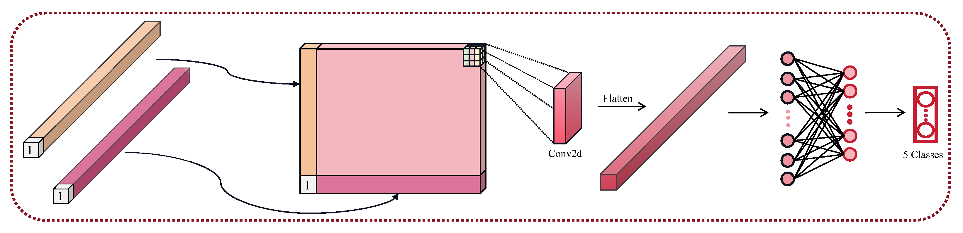
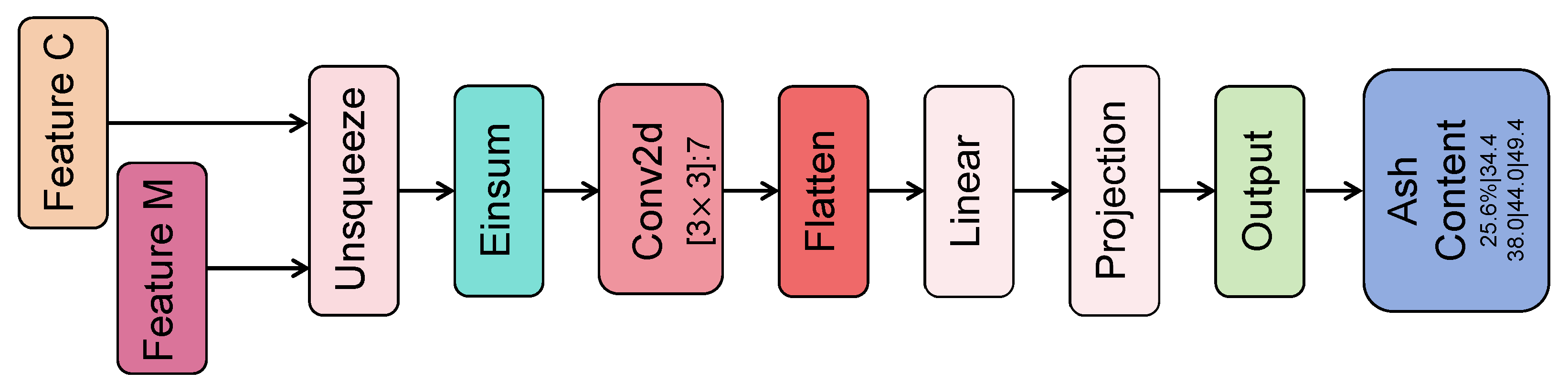
3.2.3. Fusion Convolutional Deep Classifier

After separately extracting $FeatureM$ and $FeatureC$, this paper used a fusion convolutional deep classifier to address how to effectively integrate both sets of features and mine their interrelated information. As shown in Figure 11 and Figure 12, we use two types of figures to make the description of this module clearer. In the diagram, [3 × 3]:7 indicates a convolutional kernel size of 3 × 3 with 7 output channels. To introduce feature fusion, we expand the outputs of both convolutions by appending a vector of one at the end of the features.

$$M=\mathrm{unsqueeze}\left({\mathrm{Position}}_{\mathrm{output}},2\right)$$

(20)

$$C=\mathrm{unsqueeze}\left({\mathrm{Time}}_{\mathrm{output}},1\right)$$

(21)

where M represents the expanded position-dependent feature, and C is the expanded temporal memory feature.

Figure 11. Fusion convolutional deep classifier visualization flowchart.

Figure 12. Fusion convolutional deep classifier structure diagram.

Then, by specifying the index relationship between input and output, the two corresponding feature tensors are multiplied and summed, thus achieving feature fusion.

$${\mathrm{Fusion}}_{\mathrm{output}}=einsum\left(M,C\right)$$

(22)

Further feature compression and extraction are carried out through a two-dimensional convolution layer, and the features are then flattened. The convolutional kernel size is 3, and the output channel count is 7.

$$\mathrm{Output}=\mathrm{flatten}\left(\mathrm{Conv}2d\left({\mathrm{Fusion}}_{\mathrm{output}}\right),dim=1\right)$$

(23)

Finally, through a fully connected layer and a projection layer, we map the abstracted features to the final classification results.

$${\mathrm{Final}}_{\mathrm{output}}=projection\left(\mathrm{linear}\left(\mathrm{Output}\right)\right)$$

(24)

Both sets of feature information can be fully utilized through the above method, without loss. Furthermore, the fusion of feature tensors uncovers potential connections between the two types of features, effectively capturing the input data’s complex structure and associated information.

4. Experiment

All experiments were conducted in the PyTorch 1.13.1 + CUDA 11.6 framework using an NVIDIA RTX 4090 GPU, with code implemented in Python 3.9.16. Table 2 shows some of the parameters used for model training.

Table 2. Parameters Used for Model Training.

Parameter	Value	Parameter	Value
Data Type	Univariate Sequence	Learning Rate	0.0001
Data Proportion	Balance	Batch Size	32
Data Partition	8:2	Epochs	60
Dropout Rate	0.5	Optimizer	Adam

4.1. Comparison of Preprocessing Methods

To verify the effectiveness of the ITWF, other common sequence processing methods were used for comparison. These methods included global averaging, and sliding window averaging. The original data without any function processing and data processed using a downstream time-weighted function were also compared to further validate the effectiveness. The specific formulas for each method are as follows:

Global average (GA) method, which involves directly averaging data across different time points.

$$Y_t=\frac{1}{m}\sum _{i=1}^m{x}_i$$

(25)

where m is the number of absorbance spectra, and $x_i$ represents the absorbance spectrum sequence at different time points.

Sliding window average (SWA) method, which uses a specified window size to slide through the values for averaging.

$$Y_t=\frac{1}{m}\sum _{j=1}^m\frac{1}{w}\sum _{k=i-w+1}^i{x}_i$$

(26)

where w is the size of the sliding window, j is the index of the corresponding sequence, and k is the index of elements in the sequence.

Downstream time-weighted function (DTF) method, which differs from the method in this paper by focusing on the spectral information at later time points.

$$Y_t=\frac{{\sum }_{i=1}^n{\alpha }^{n-i}{x}_i}{{\sum }_{i=1}^n{\alpha }^{n-i}}$$

(27)

Original dataset (OD) method, without any defined function processing.

Table 3 and Figure 13 present the detection results of the methods. The experimental results showed that our method (ITWF) performed the best, followed by Method B (sliding window average), then Method A (global average), followed by Method D (original dataset without defined function processing), and finally Method C (downstream time-weighted function). Our method was the most effective in dealing with the sedimentation phenomenon in suspension samples. Because the ITWF emphasized data from earlier time points, it better captured the differential information of the suspension samples at the initial moment. This method excels in handling the richness of information in dynamic processes. The poorer performance of the other methods can be attributed to their varying degrees of neglect for the dynamic nature of spectral feature changes.

Table 3. Comparison of five preprocessing methods.

Methods	Accuracy	F1-Score	Precision	Recall
GA	0.6452	0.6301	0.6333	0.6548
SWA	0.7424	0.7343	0.7564	0.7452
DTF	0.6323	0.6207	0.6241	0.6314
OD	0.6774	0.6703	0.6710	0.6833
ITWF	0.8065	0.8045	0.8343	0.8065

Figure 13. Preprocessing method visualization.

4.2. Model Comparison Experiment

Additionally, we evaluated several typical methods of coal identification [29], which included random forest (RF), support vector machine (SVM), extreme learning machine (ELM), tensor extreme learning machine (TELM), PCA-ELM (principal component analysis for extreme learning machine), and convolutional neural network with extreme learning machine (CNN + ELM) methods. The CNN + ELM method was adapted from [29]. Originally designed for two-dimensional image data, we modified it to accommodate one-dimensional data dimensions. Figure 14 illustrates its network structure. In the diagram, [1 × 3]:32 indicates that the convolutional kernel size was 1 × 3 with 32 output channels, and so on. Furthermore, we compared some representative time-series networks: LSTM [34], TCN (temporal convolutional network) [35], and Transformer [36]. We evaluated each method based on four key performance metrics: accuracy, F1 score, precision, and recall, to validate the superiority of the model proposed in this paper.

Figure 14. CNN + ELM network architecture.

As shown in Table 4 and Figure 15, firstly, from an overall perspective, significant differences were observed in the performance of the various methods across the four evaluation metrics: accuracy, F1 score, precision, and recall. These metrics are key factors in measuring the performance of machine learning models and collectively determine a model’s overall effectiveness. Our approach demonstrated the best performance across all four metrics among these methods. RF and SVM performed relatively poorly, indicating their limited adaptability to the data. TELM and ELM exhibited a similar performance, with TELM showing slight improvements in precision and recall. PCA_ELM underperformed compared to ELM, suggesting that PCA did not significantly enhance ELM’s performance in this context. The LSTM model’s performance was average, particularly lacking in accuracy and F1-score. The TCN model showed good performance in terms of precision. Both the CNN + ELM and Transformer models performed well across all metrics.

Table 4. Comparison of model results.

Methods	Accuracy	F1-Score	Precision	Recall
RF	0.6581	0.6392	0.6565	0.6433
SVM	0.6193	0.6086	0.6108	0.6233
ELM	0.7548	0.7549	0.7554	0.7548
TELM	0.7545	0.7556	0.7615	0.7599
PCA_ELM	0.7161	0.7188	0.7191	0.7209
CNN + ELM	0.7871	0.7849	0.7831	0.7871
LSTM	0.6839	0.6736	0.7023	0.6839
TCN	0.7201	0.7167	0.7842	0.7205
Transformer	0.7742	0.7514	0.8089	0.7571
DSFN	0.8065	0.8045	0.8343	0.8065

Figure 15. Performance metric visualization.

4.3. Ablation Study

To verify the effectiveness of the improved MSCR module and CLSM-CS module, we conducted ablation experiments, as shown in Table 5. In these experiments, DSFN-A represents the model without the MSCR module (replaced by a single convolutional layer with a kernel size of 3), DSFN-B represents the model without the CLSM-CS module (replaced by LSTM with the same input parameters), and DSFN-AB indicates the model with both modules removed. It is evident that the MSCR module and the CLSM-CS module were effective in improving the model performance, with the best results achieved through their synergistic interaction.

Table 5. Ablation Results.

Methods	Accuracy	F1-Score	Precision	Recall
DSFN-A	0.7552	0.7554	0.7574	0.7560
DSFN-B	0.7806	0.7801	0.7934	0.7806
DSFN-AB	0.7345	0.7331	0.7335	0.7345
DSFN	0.8065	0.8045	0.8343	0.8065

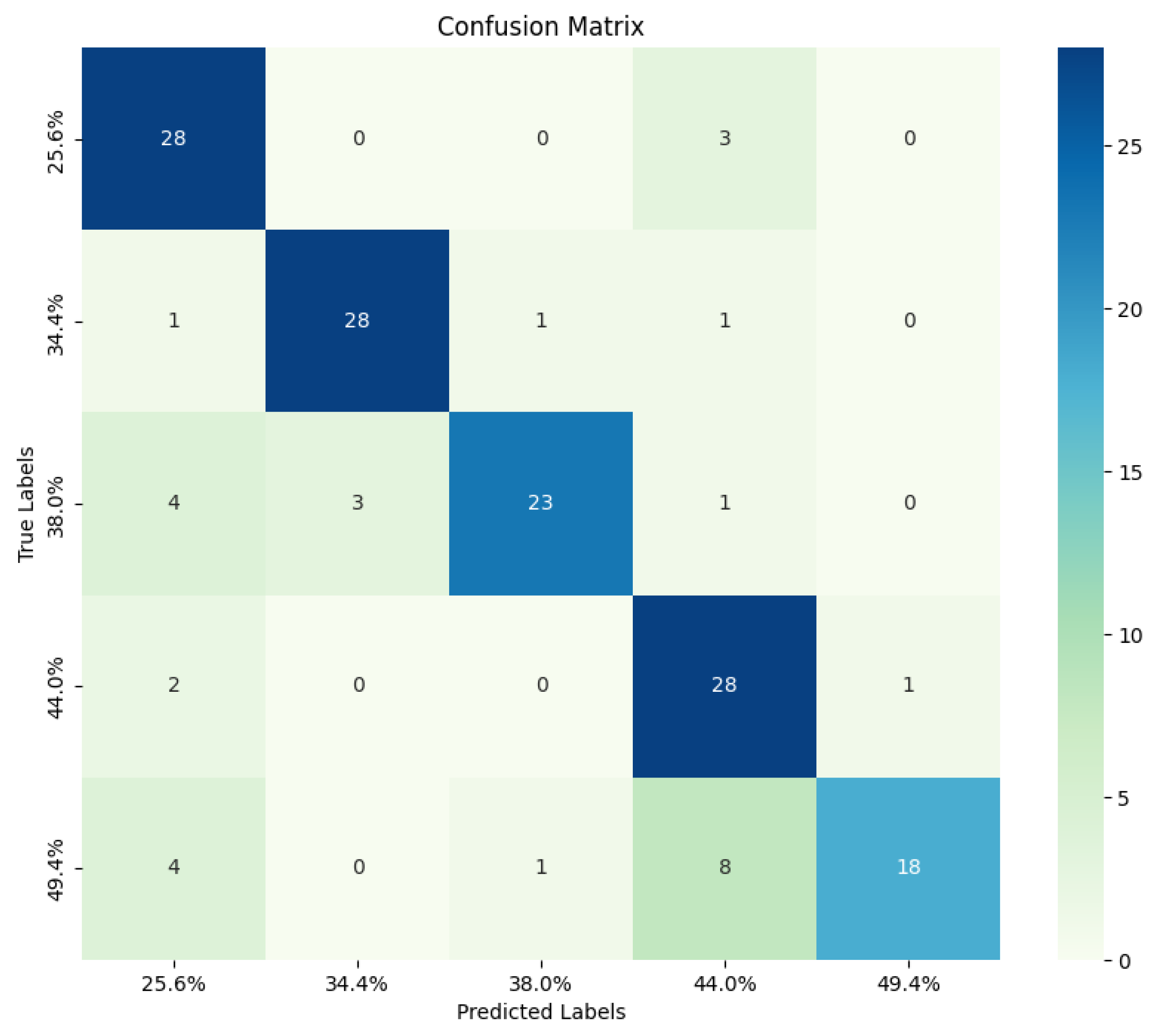
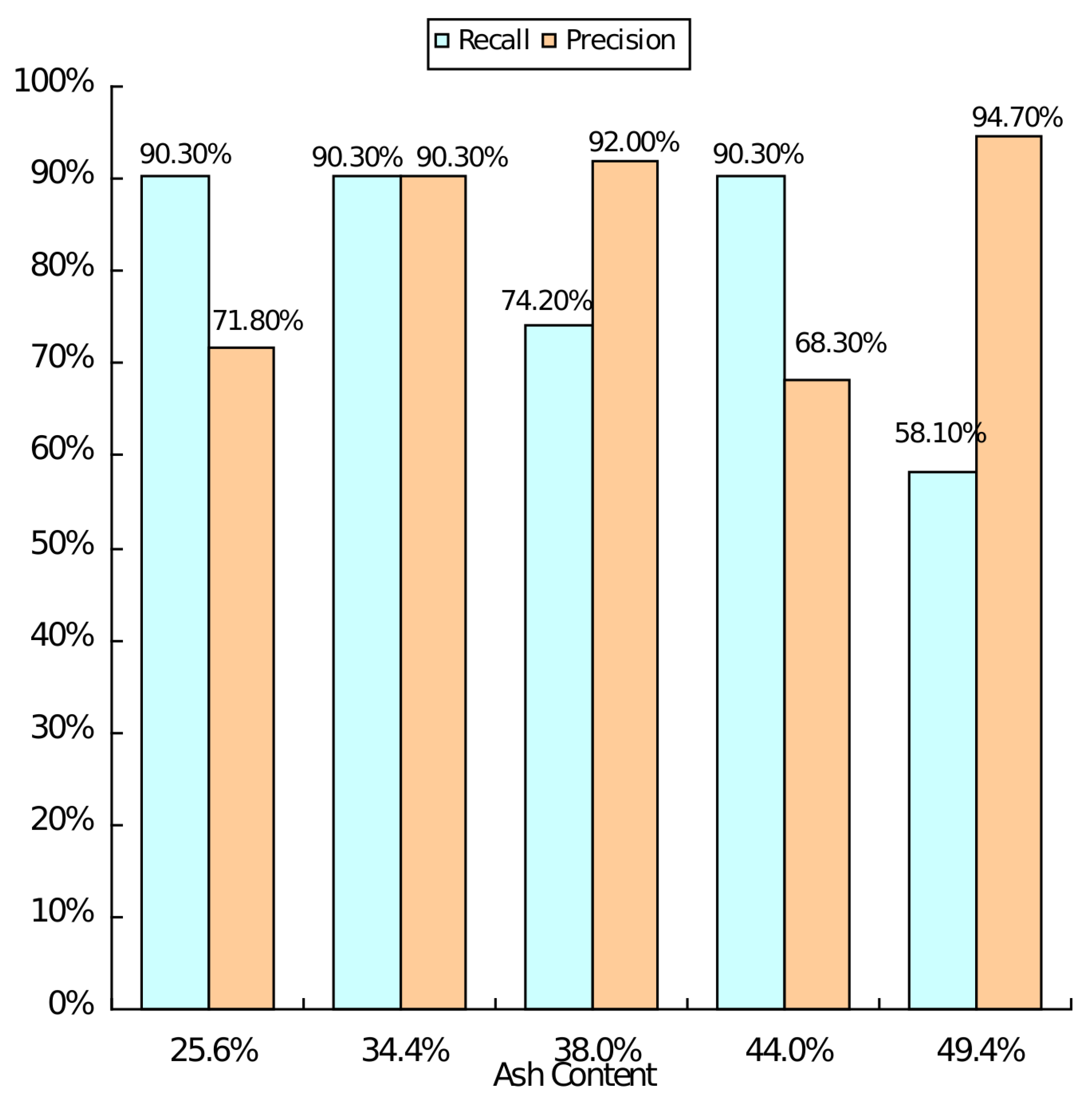
4.4. Performance Evaluation of Each Category

Lastly, we also examined the model’s performance in individual categories rather than overall effectiveness. Figure 16 presents a confusion matrix, commonly used for evaluating classification models. The horizontal axis denotes the model’s predicted labels, while the vertical axis represents the true labels. The intensity of colors reflects sample quantities, with darker shades indicating higher counts. It is evident that the model accurately classified the majority of samples. In Figure 17, we depict the recall and precision for each category separately, highlighting the model’s most precise detection for the 34.4% category. However, the model exhibited a tendency to confuse similar categories, as illustrated in Figure 15, where a significant proportion of samples, originally labeled as 49.4%, were misclassified as 44.0%. Addressing this limitation represents one of the areas for future improvement.

Figure 16. Confusion matrix of model prediction.

Figure 17. Prediction of different ash contents.

5. Discussion

Our method presents a tailored approach by directing its focus towards analyzing the absorption spectra of coal slurry flotation tailings. To tackle the sedimentation issue observed in samples, it puts forward the concept of ITWF. This innovative function aims to highlight the characteristics of early-time data, while retaining valuable late-time information. Additionally, we designed the DSFN (DeepSpectraFusionNet) model to specifically extract features from our data. The experimental findings further underscored the method’s efficacy and superiority. This marks the first proposal in the field of detecting ash content in coal slurry flotation tailings, offering a fresh perspective for research.

Limitations: Although this study demonstrated certain advantages compared to conventional methods, from data selection to model design, we must also acknowledge its limitations. Firstly, concerning data selection, the presence of sedimentation phenomena necessitated a sampling duration of at least approximately 5 min per data point, which still falls short of the ideal requirements for rapid industrial testing. Then, while particles in the suspended liquid samples tended to settle over time, they still exhibited random movements, and capturing information about the random motion of sample particles while discarding redundant information is a major challenge in model design. Additionally, the industrial setting requires smaller and faster model structures, and our model still has some gaps in meeting these needs. To address these fundamental issues, future research will focus on redesigning and optimizing the sampling platform, to achieve faster, smaller, and more accurate detection methods.

6. Conclusions

Addressing the stability issues associated with traditional image detection methods, this paper focused on the state of flotation tailings coal suspensions as the research subject. Utilizing a microfiber-optic spectrometer to collect absorbance spectrum data reduced the dependency on external conditions and enhanced industrial adaptability. A rapid detection method for coal ash content in tailings suspension based on absorption spectra and deep feature extraction was proposed. The ITWF emphasized the inherent connection of sample sedimentation, enhancing the model’s ability to learn spectral temporal memory features. We designed a DSFN model to specifically extract relevant features. Using the MSCR module enabled the model to extract strongly correlated positional information between adjacent wavelengths in the spectrum. In contrast, introducing the CLSM-CS module strengthened the capturing of local information and temporal memory. Finally, applying a fusion convolutional deep classifier effectively merged temporal memory features with position-dependent features, creating a precise ash content detection correlation model. The experimental results demonstrated the method’s high stability, accuracy, and rapidity in industrial field applications, showcasing its immense potential in tailings coal ash content detection.

References

- Liang, H.; Li, Y. Analyses of influencing factors of fine coal flotation. Coal Process. Compr. Util. 2023, 20–24. [Google Scholar] [CrossRef]
- Fookes, R.; Gravitis, V.; Watt, J.; Hartley, P.; Campbell, C.; Howells, E.; McLennan, T.; Millen, M. On-line determination of the ash content of coal using a “Siroash” gauge based on the transmission of low and high energy γ-rays. Int. J. Appl. Radiat. Isot. 1983, 34, 63–69. [Google Scholar] [CrossRef]
- Vardhan, R.H.; Giribabu. On-Line Coal-Ash Monitoring Technologies in Coal Washaries—A Review. Procedia Earth Planet. Sci. 2015, 11, 49–55. [Google Scholar] [CrossRef]
- Li, J.; Zhang, J.; Ge, L.; Zhou, W.; Zhong, D. Software design method and application of Monte Carlo simulation of NaI detector natural γ spectrum. Nucl. Electron. Detect. Technol. 2005, 423–425. [Google Scholar]
- Huang, X.; Wang, G.; Sun, P.; Yang, D.; Ma, Y. Low-energy γ-ray backscatter method for measuring coal ash. Nucl. Tech. 2005, 72–75. [Google Scholar]
- Bona, M.; Andrés, J. Coal analysis by diffuse reflectance near-infrared spectroscopy: Hierarchical cluster and linear discriminant analysis. Talanta 2007, 72, 1423–1431. [Google Scholar] [CrossRef]
- Gui, W.; Yang, C.; Xu, D.; Lu, M.; Xie, Y. Research progress on mineral flotation process monitoring technology based on machine vision. Acta Autom. Sin. 2013, 39, 1879–1888. [Google Scholar] [CrossRef]
- Zhao, B.; Hu, S.; Zhao, X.; Zhou, B.; Li, J.; Huang, W.; Chen, G.; Wu, C.; Liu, K. The application of machine learning models based on particles characteristics during coal slime flotation. Adv. Powder Technol. 2022, 33, 103363. [Google Scholar] [CrossRef]
- Tan, L.; Zhang, Z.; Zhao, W.; Zhang, R.; Zhang, K. Research progress on mineral flotation foam monitoring based on machine vision. Min. Res. Dev. 2020, 40, 123–130. [Google Scholar] [CrossRef]
- Wang, J.; Wang, R.; Fu, X.; Wu, T. Research on soft measurement of flotation tail coal ash based on color image processing. Coal Eng. 2020, 52, 137–142. [Google Scholar]
- Ding, J.; Bai, F.; Ren, X.; Fan, M. Ash content prediction system of clean coal based on flotation foam image recognition. Coal Prep. Technol. 2022, 50, 89–93. [Google Scholar] [CrossRef]
- Guo, X.; Wei, L.; Yang, C. Study on coal slime flotation tailings ash detection method based on deep convolutional network. Coal Technol. 2020, 39, 144–146. [Google Scholar] [CrossRef]
- Wen, Z.; Zhou, C.; Pan, J.; Nie, T.; Zhou, C.; Lu, Z. Deep learning-based ash content prediction of coal flotation concentrate using convolutional neural network. Miner. Eng. 2021, 174, 107251. [Google Scholar] [CrossRef]
- Yang, X.; Zhang, K.; Ni, C.; Cao, H.; Thé, J.; Xie, G.; Tan, Z.; Yu, H. Ash determination of coal flotation concentrate by analyzing froth image using a novel hybrid model based on deep learning algorithms and attention mechanism. Energy 2022, 260, 125027. [Google Scholar] [CrossRef]
- Han, Y.; Wang, L.; Liu, Q.; Gui, X. Intelligent detection method of flotation tail coal ash based on CNN-BP. Ind. Min. Autom. 2023, 49, 100–106. [Google Scholar] [CrossRef]
- Manley, M. Near-infrared spectroscopy and hyperspectral imaging: Non-destructive analysis of biological materials. Chem. Soc. Rev. 2014, 43, 8200–8214. [Google Scholar] [CrossRef] [PubMed]
- Yang, J.; Wang, J.; Lu, G.; Fei, S.; Yan, T.; Zhang, C.; Lu, X.; Yu, Z.; Li, W.; Tang, X. TeaNet: Deep learning on Near-Infrared Spectroscopy (NIR) data for the assurance of tea quality. Comput. Electron. Agric. 2021, 190, 106431. [Google Scholar] [CrossRef]
- Chang, Y.T.; Hsueh, M.C.; Hung, S.P.; Lu, J.M.; Peng, J.H.; Chen, S.F. Prediction of specialty coffee flavors based on near-infrared spectra using machine-and deep-learning methods. J. Sci. Food Agric. 2021, 101, 4705–4714. [Google Scholar] [CrossRef] [PubMed]
- Li, X.; Fan, P.; Li, Z.; Chen, G.; Qiu, H.; Hou, G. Soil classification based on deep learning algorithm and visible near-infrared spectroscopy. J. Spectrosc. 2021, 2021, 1508267. [Google Scholar] [CrossRef]
- Xiao, D.; Vu, Q.H.; Le, B.T. Salt content in saline-alkali soil detection using visible-near infrared spectroscopy and a 2D deep learning. Microchem. J. 2021, 165, 106182. [Google Scholar] [CrossRef]
- Liu, J.; Zhang, J.; Tan, Z.; Hou, Q.; Liu, R. Detecting the content of the bright blue pigment in cream based on deep learning and near-infrared spectroscopy. Spectrochim. Acta Part A Mol. Biomol. Spectrosc. 2022, 270, 120757. [Google Scholar] [CrossRef] [PubMed]
- Bai, X.; Zhang, L.; Kang, C.; Quan, B.; Zheng, Y.; Zhang, X.; Song, J.; Xia, T.; Wang, M. Near-infrared spectroscopy and machine learning-based technique to predict quality-related parameters in instant tea. Sci. Rep. 2022, 12, 3833. [Google Scholar] [CrossRef] [PubMed]
- Ravichandran, P.; Viswanathan, S.; Ravichandran, S.; Pan, Y.J.; Chang, Y.K. Estimation of grain quality parameters in rice for high-throughput screening with near-infrared spectroscopy and deep learning. Cereal Chem. 2022, 99, 907–919. [Google Scholar] [CrossRef]
- Lee, P.H.; Torng, C.C.; Lin, C.H.; Chou, C.Y. Control chart pattern recognition using spectral clustering technique and support vector machine under gamma distribution. Comput. Ind. Eng. 2022, 171, 108437. [Google Scholar] [CrossRef]
- Ma, Y.; Lan, Y.; Xie, Y.; Yu, L.; Chen, C.; Wu, Y.; Dai, X. A Spatial–Spectral Transformer for Hyperspectral Image Classification Based on Global Dependencies of Multi-Scale Features. Remote Sens. 2024, 16, 404. [Google Scholar] [CrossRef]
- Le, B.T.; Xiao, D.; Mao, Y.; He, D. Coal analysis based on visible-infrared spectroscopy and a deep neural network. Infrared Phys. Technol. 2018, 93, 34–40. [Google Scholar] [CrossRef]
- Mao, Y.; Le, B.T.; Xiao, D.; He, D.; Liu, C.; Jiang, L.; Yu, Z.; Yang, F.; Liu, X. Coal classification method based on visible-infrared spectroscopy and an improved multilayer extreme learning machine. Opt. Laser Technol. 2019, 114, 10–15. [Google Scholar] [CrossRef]
- Xiao, D.; Le, B.T. Rapid analysis of coal characteristics based on deep learning and visible-infrared spectroscopy. Microchem. J. 2020, 157, 104880. [Google Scholar] [CrossRef]
- Xiao, D.; Le, T.T.G.; Doan, T.T.; Le, B.T. Coal identification based on a deep network and reflectance spectroscopy. Spectrochim. Acta Part A Mol. Biomol. Spectrosc. 2022, 270, 120859. [Google Scholar] [CrossRef]
- Xiao, D.; Yan, Z.; Li, J.; Fu, Y.; Li, Z. Rapid proximate analysis of coal based on reflectance spectroscopy and deep learning. Spectrochim. Acta Part A Mol. Biomol. Spectrosc. 2023, 287, 122042. [Google Scholar] [CrossRef]
- Li, B.; Xiao, D.; Xie, H.; Huang, J.; Yan, Z. Coal Classification Based on Reflection Spectroscopy and the IAT-TELM Algorithm. ACS Omega 2023, 8, 35232–35241. [Google Scholar] [CrossRef]
- Li, Z.; Wang, D.; Zhu, T.; Ni, C.; Zhou, C. SCNet: A deep learning network framework for analyzing near-infrared spectroscopy using short-cut. Infrared Phys. Technol. 2023, 132, 104731. [Google Scholar] [CrossRef]
- Hua, Y.; Zhao, Z.; Li, R.; Chen, X.; Liu, Z.; Zhang, H. Deep learning with long short-term memory for time series prediction. IEEE Commun. Mag. 2019, 57, 114–119. [Google Scholar] [CrossRef]
- Yu, Y.; Si, X.; Hu, C.; Zhang, J. A review of recurrent neural networks: LSTM cells and network architectures. Neural Comput. 2019, 31, 1235–1270. [Google Scholar] [CrossRef] [PubMed]
- Bai, S.; Kolter, J.Z.; Koltun, V. An empirical evaluation of generic convolutional and recurrent networks for sequence modeling. arXiv 2018, arXiv:1803.01271. [Google Scholar]
- Lin, T.; Wang, Y.; Liu, X.; Qiu, X. A survey of transformers. AI Open 2022, 3, 111–132. [Google Scholar] [CrossRef]
Disclaimer/Publisher’s Note: The statements, opinions and data contained in all publications are solely those of the individual author(s) and contributor(s) and not of MDPI and/or the editor(s). MDPI and/or the editor(s) disclaim responsibility for any injury to people or property resulting from any ideas, methods, instructions or products referred to in the content. |
© 2024 by the authors. Licensee MDPI, Basel, Switzerland. This article is an open access article distributed under the terms and conditions of the Creative Commons Attribution (CC BY) license (https://creativecommons.org/licenses/by/4.0/).