Abstract
Simulating the probability of type I error is a powerful statistical tool that allows confirming if the statistical test achieves the established nominal level. However, its computational implementation has the drawback of significantly long execution times. Therefore, this article analyzes the performance of two parallel implementations (parRapply and boot) which significantly reduce the execution time of simulations of type I error probability for a goodness-of-fit test for the bivariate Poisson distribution. The results obtained demonstrate how the parallelization strategies accelerate the simulations, reducing the time by 50% to 90% when using 2 to 12 processors running in parallel. This reduction is graphically evidenced as the execution time of the analyzed parallel versions fits almost perfectly () to the power model , where p is the number of processors used, and  and  are the constants of the model. Furthermore, it is shown that the parallelization strategies used scale with an increasing number of processors. All algorithms were implemented in the R programming language, and their code is included at the end of this article.
    MSC:
                62-08
            1. Introduction
In today’s world, it is essential to anticipate events that may occur, and to do so, having models that predict such events with the highest possible accuracy is vital. Statistics provides tools for making predictions or decisions based on the information contained in the available data sample. Typically, these tools consist of models based on probability distributions. However, before using such models, it is crucial to determine whether the sample data behave according to the probability distribution on which the probabilistic model is based. This is achieved by applying a goodness-of-fit test.
Regarding the latter, it is necessary to specify that an essential part in the development of a goodness-of-fit test is the result of simulation under the null hypothesis, which confirms if the test reaches the established nominal level. In [], two goodness-of-fit tests were generated, and the parametric bootstrap method was used to simulate the type I error probability. However, the excessive execution time of each simulation influenced the authors to make a few variations in both the parameter vector  and the sample sizes n considered.
In this regard, to explore more and new possible scenarios, it is fundamental and necessary to reduce the computational execution time of the involved simulation processes. Many areas pursue this goal and employ parallel programming for it, for instance in [,,,,,].
Therefore, the interest of this research is to use parallelization strategies to accelerate the simulation processes employed in the first of the statistical tests developed in []. This will allow examining new parameters  and testing with larger sample sizes n. It will contribute to reducing computation time and confirming that as sample sizes grow, parameter estimates converge to their nominal value.
This article is organized as follows: Section 2 presents the theoretical aspects and details the first test proposed in []. Section 3 shows the fundamental aspects to take into account to implement a parallel algorithm and are discussed the facilities offered by the R language to make implementations of this type. Section 4 presents the experimental results. In Section 5, the obtained results are discussed, and Section 6 exhibits the conclusions.
2. Background
From here on, the following notation is considered:
- .
 - .
 
2.1. Bivariate Poisson Distribution
There have been several definitions for the bivariate Poisson distribution. This article utilizes the data provided in [], which is the one that has received the most attention in the statistical literature.
Definition 1. 
  Let


    where  and  are mutually independent Poisson random variables with means given by ,  and , respectively.
The joint distribution of the vector  is called bivariate Poisson distribution with parameter , which will be denoted by .
The joint probability mass function of  and  is given by


    where .
Also, the joint probability generating function (pgf) of  and  is


, .
2.2. Goodness-of-Fit Test of Novoa-Muñoz and Jiménez-Gamero (2014)
This subsection shows, in summary, the first test proposed by these authors, hereinafter, test Q.
To do this, let  be random vectors independent and identically distributed of .
The hypotheses are contrasted


According to the definition established in [], if  but the hypothesis test incorrectly decides to reject , then the test has made a type I error.
The test statistic is of the Cramer Von Misses type and is given by


        where a consistent estimator  is a consistent estimator of ,  is the pgf and  its empirical version,  is the weight function, in which  and , called the weight vector, is such that .
The null hypothesis will be rejected for “large” values of .
Since the null distribution of the statistic turned out to be unknown, the authors estimated it using the asymptotic null distribution, but since it depends on the true value of the  parameter, which is unknown, it did not provide them will a useful solution and decided to estimate the null distribution of the statistic using the parametric bootstrap method, which is analyzed below.
2.3. Parametric Bootstrap
In the case under study, the distribution of the statistic depends on the parameter; then, such a model is called parametric, and therefore, the statistical methods based in this model are parametric methods [].
As in the real world, a sample from a given population is obtained, and with this sample, the population parameter is estimated, which is expected to be an interior point of the parameter space. The parametric bootstrap method is a resampling technique that emulates the situation described above; that is, with the parameter estimator, a Bivariate Poisson is generated from which a sample is drawn, called the bootstrap sample, and with it the parameter is estimated, which is named the bootstrap parameter. With the sample and the bootstrap parameter, the statistic  is computed, which is the bootstrap version of the statistic Q.
Although the bootstrap method has been highly useful in statistical inference, [] shows that there are situations in which it is not consistent. In the said article, examples are shown where parametric bootstrap does not yield good results, and particularly, it is demonstrated that the method is inconsistent when the true parameter value is on the boundary of the parameter space or very close to it.
3. A Parallel Implementation
There are two parameters to analyze the efficiency of an algorithm which solves a given problem: the memory space required to store the input data and results and the time of execution used in performing the task. Several technological advances allow the use of many computers that collaborate each other either to increase the size of problems to be solved through data distribution or task distribution []. In this latter case, parallel programs are being used. In the case of bootstrap resampling, it involves task distribution, as the iterations are independent of each other.
3.1. Parallelization in R Language
The R programming language offers the possibility of developing tasks in parallel, when they allow it, through a series of packages that provide commands for this type of processing. Among the packages that help accomplish this task, Snow, Multicore, and Parallel can be mentioned.
Currently, one of the packages that has gained great prominence in the programming in R language is Parallel [], which takes the best of two previous versions Multicore and Snow, which is complemented by the random numbers generation [,].
The parApply package allows all the functions contained in Apply, such as the direct data manipulation from each vector data, matrix, list or data frames avoiding the use of cycles. It also allows finding out how many processors are available.
Thus, the parallel package allows distributing the data in the different cores available and there, simultaneously, manipulating them according to the indicated function, and then gathering all the information and returning it as a list [].
In general terms, two ways of implementing parallelism using this package can be distinguished: through forking or sockets.
The forking method is based on the full duplication of a master process with a shared environment toward each of the parallel environments, including objects or variables defined before the start of parallel threads. This method has the advantage of being very fast, but it cannot run under the Windows operating system.
On the other hand, the sockets method is based where each thread runs separately without sharing objects or variables, which can only be passed from the master process explicitly. As a result, it runs slower due to communication overhead, but it has the advantage of being able to be implemented in any operating system [].
Just as the Parallel package offers tools that allow parallelization in R, there is a Boot package [] that incorporates functions that facilitate the application of the bootstrap method. For this package, we consider the possibility of performing the operations in parallel using forking or a socket.
When programming in parallel in R language [], with the aim of reducing computation times, it is important to take into account some experts’ recommendations. In many cases, simply “quite fast” is pretty good. The additional speed that could be achieved by transitioning from R to C/C++ does not justify the significant amount of time required to write, debug, and maintain code at that level [].
3.2. Performance Evaluation of a Parallel Program
According to [], one way to measure the performance of a parallel program is to calculate its Speedup (S), which is the ratio between the execution time of the program in the sequential version () and the execution time of the parallel version () with p processors, which is given by .
Furthermore, as the processors used increase, there is more additional work (and time) than expected; that is, the ratio between S and p decreases in value. Thus, the Efficiency of a parallel program is defined as .
3.3. Methodology
To showcase the results of this work, three aspects are considered:
- (a)
 - Preparation of the programs.Once it was verified that the process was parallelizable, the parts of the program that could be modified to reduce computation times were identified; then, the instructions of the R language that allow for parallelizing the task were analyzed, finding parRapply from the package Parallel, and boot from the Boot package. Then, the new codes that allow for parallelizing the simulation process were developed.
 - (b)
 - Simulation with the same components used in []. The simulations made by these authors were replicated considering the execution sequential and parallel code. For the parallel program, the number of cores p, using .
 - (c)
 - Simulations with new components.
- -
 - New weight vectors , with .
 - -
 - Sample sizes with the same original population parameters and .
 - -
 - Population parameters , with , and chosen so that the correlation coefficient is less than 0.25 or greater than 0.75, and .
 
 
The simulations described in items (b) and (c) were carried out in a cluster of computers with 12 processors with a processing speed of 2.00 GHz, 32 GB of RAM and operating system Centos 7 (Linux).
4. Experimental Results
This section presents the results of the simulations of type I error considering the three parts detailed in  Section 3.3.
4.1. Simulations of Probability of a type I error with the Components Used in the First Test of Novoa-Muñoz and Jiménez-Gamero (2014)
Firstly, it was verified that when using parallel programming, there was no significant difference between the simulated type I error probability and its respective nominal value. Due to space, the results are not presented in this paper and can be obtained from the author upon request.
The next step was to analyze the execution times and the efficiency of the two parallel versions (parRapply and boot commands). For this, it is essential to know the sequential execution time, which is presented in Table 1 and Table 2. Table 1 presents the results using the algorithm implemented in this research (described in Appendix A), and Table 2 records the results of running the R package 4.0.0 boot command. These times serve as a basis for calculating the performance of parallel programming.
       
    
    Table 1.
    Average execution time (in seconds) using Sequential Version, weight vectors , sample sizes n and parameters .


    Table 2.
    Average execution time (in seconds) using boot Sequential Version, weight vectors , sample sizes n and parameters .
  
The execution times and efficiency of the parallelized programs using the parRapply and boot commands, which were the two parallel versions analyzed in this study, are shown graphically below.
Figure 1, Figure 2, Figure 3, Figure 4, Figure 5 and Figure 6 present the average execution times versus the number of processors used. To obtain these results and for comparison, the same parameters  used in [] were used. Table A1–Table A12, displayed in Appendix B, contain the data with which these graphs were constructed.
      
    
    Figure 1.
      Average execution time (in seconds) using parRapply and boot commands versus number of processors p and different sample sizes n for  (1, 1, 0.75).


    Figure 2.
      Average execution time (in seconds) using parRapply and boot commands versus number of processors p and different sample sizes n for  (1, 1, 0.50).


    Figure 3.
      Average execution time (in seconds) using parRapply and boot commands versus number of processors p and different sample sizes n for  (1, 1, 0.25).


    Figure 4.
      Average execution time (in seconds) using parRapply and boot commands versus number of processors p and different sample sizes n for  (1.5, 1, 0.62).


    Figure 5.
      Average execution time (in seconds) using parRapply and boot commands versus number of processors p and different sample sizes n for  (1.5, 1, 0.92).


    Figure 6.
      Average execution time (in seconds) using parRapply and boot commands versus number of processors p and different sample sizes n for  (1.5, 1, 0.31).
  
Figure 1, Figure 2 and Figure 3 show the execution times when  and Figure 4, Figure 5 and Figure 6 show the times when .
Since in this research two parallel implementations are analyzed, the interest lies in knowing which of them is more efficient; therefore, the efficiencies of both parallel implementations were calculated. Figure 7, Figure 8, Figure 9, Figure 10, Figure 11 and Figure 12 display the efficiencies, E, versus the number of processors used. Each figure shows graphically the efficiency of both commands (parRapply and boot) for the same parameter . These parameters are the same ones used in [].
      
    
    Figure 7.
      Efficiency of running the parRapply and boot commands versus number of processors p and different sample sizes n for  (1, 1, 0.75).


    Figure 8.
      Efficiency of running the parRapply and boot commands versus number of processors p and different sample sizes n for  (1, 1, 0.50).


    Figure 9.
      Efficiency of running the parRapply and boot commands versus number of processors p and different sample sizes n for  (1, 1, 0.25).


    Figure 10.
      Efficiency of running the parRapply and boot commands versus number of processors p and different sample sizes n for  (1.5, 1, 0.62).


    Figure 11.
      Efficiency of running the parRapply and boot commands versus number of processors p and different sample sizes n for  (1.5, 1, 0.92).


    Figure 12.
      Efficiency of running the parRapply and boot commands versus number of processors p and different sample sizes n for  (1.5, 1, 0.31).
  
Tables with these data are not shown, as they can be obtained directly using Table 1 and Table 2 (sequential time) together with Table A1–Table A12 in Appendix B (parallel time).
4.2. Simulations of Type I Error Probability with Sample Sizes Larger than Those Used in the First Test of Novoa-Muñoz and Jiménez-Gamero (2014)
For simulations with sample sizes greater than  70, only the command parRapply was used because, as seen in the previous subsection, it is more efficient than the command boot. Furthermore, only ten processors were used.
The estimations of the type I error probabilities for the nominal values  = 0.01, 0.05, and 0.10 are presented in Table 3, Table 4, Table 5, Table 6, Table 7 and Table 8 with 1%, 5% and 10%, respectively.
       
    
    Table 3.
    Results of simulating probability of type I error. Instance .


    Table 4.
    Results of simulating probability of type I error. Instance .


    Table 5.
    Results of simulating probability of type I Error. Instance .


    Table 6.
    Results of simulating probability of type I error. Instance .


    Table 7.
    Results of simulating probability of type I error. Instance .


    Table 8.
    Results of simulating probability of type I error. Instance .
  
Figure 13 and Figure 14 present the average execution times versus different sample sizes (n) when the simulations displayed in Table 3, Table 4, Table 5, Table 6, Table 7 and Table 8 are executed.
      
    
    Figure 13.
      Average execution time (in seconds) versus sample sizes n for parameters  when .


    Figure 14.
      Average execution time (in seconds) versus sample sizes n for parameters  when .
  
4.3. Simulations of the Probability of a Type I Error with Parameter Vectors Different from Those Used in the First Test of Novoa-Muñoz and Jiménez-Gamero (2014)
The simulation of type I errors implemented in parallel allows to evaluate the performance of the Q test when working with vectors that have parameters different to those already studied. In particular, it allows simulating the type I error probability for the cases in which the correlation coefficient  takes very small (≤ 0.1) or very large (≥ 0.8) values. The first of these cases takes on special relevance, since it involves parameters that are very close to the boundary of the parametric space, which according to [] could lead to inconsistencies while increasing computation times.
For the same reasons given in Section 4.2, only the command parRapply and ten processors were used.
Table 9, Table 10, Table 11, Table 12, Table 13, Table 14 and Table 15 present the results of the type I error simulation for the parameter vectors that meet the characteristics already mentioned, considering the cases  and  with the following sample sizes , and 200.
       
    
    Table 9.
    Results of simulating probability of type I error. Instance .


    Table 10.
    Results of simulating probability of type I error. Instance .


    Table 11.
    Results of simulating probability of type I error. Instance .


    Table 12.
    Results of simulating probability of type I error. Instance .


    Table 13.
    Results of simulating probability of type I error. Instance .


    Table 14.
    Results of simulating probability of type I error. Instance .


    Table 15.
    Results of simulating probability of type I error. Instance .
  
Figure 15 and Figure 16 present the average execution times versus different sample sizes (n) when the simulations displayed in Table 9, Table 10, Table 11, Table 12, Table 13, Table 14 and Table 15 are executed.
      
    
    Figure 15.
      Average execution time (in seconds) versus sample sizes n for parameters  when .


    Figure 16.
      Average execution time (in seconds) versus sample sizes n for parameters  when .
  
5. Discussion
From Table 1 and Table 2, it is evident that the sequential version implemented in this research is faster (between 1% and 2%) than the boot version of the R package in almost all parameters , except for  (1.5, 1, 0.92). This could be attributed to the sensitivity of the Maximum Likelihood Method, as  is very close to .
On the other hand, regardless of the parallel version (parRapply or boot) used, Figure 1, Figure 2, Figure 3, Figure 4, Figure 5 and Figure 6 highlight the rapid decrease in program execution time as the number of processors increases. Additionally, it is observed that the parRapply command delivers results faster than the boot command. Furthermore, when , the execution time is lower than in cases where . It is observed that the execution time increases as sample sizes grow.
It is also important to emphasize that the power model (faster than the exponential model) fits almost perfectly to the execution time versus number of processors, as approximately 99.9% () of the variation in execution time is explained by the number of processors used.
Adding to the previous point, Figure 7, Figure 8, Figure 9, Figure 10, Figure 11 and Figure 12 show that the two parallel implementations addressed in this research exhibit linear efficiency. In all analyzed cases, the parRapply command is more efficient than the boot command and with less dispersion among the sample sizes used. Furthermore, it is observed that when two processors are employed, the efficiency of the parRapply command is superior to 1.
In this line of discussion and thanks to this research (using parallel programming), it was possible to obtain results for sample sizes greater than 70, which are displayed in Table 3, Table 4, Table 5, Table 6, Table 7 and Table 8. From these tables, it can be observed that the estimates are close to the nominal values. For example, the estimates at 10% are very close to 0.1. This becomes clearer as the sample size increases, implying that the estimates are converging to the nominal values.
In line with the previous paragraph, Figure 13 and Figure 14 graphically illustrate the positive correlation between the execution time of the programs and the sample size. Clearly, the execution time of the programs is linearly adjusted with the sample size, and this adjustment is almost perfect (). It is also evident that the execution time of the programs is lower when .
Finally, from Table 9, Table 10, Table 11, Table 12, Table 13, Table 14 and Table 15, it is possible to appreciate that the estimations of the type I error probability are very close to the nominal values in all cases where the correlation coefficient . However, as could be expected, according to what [] suggested, in the cases in which  and  (), the simulated probabilities are very far from the nominal values and, strangely, the situation worsens as the sample size grows.
In relation to the last paragraph, from Figure 15 and Figure 16, it is appreciated that the execution time of the programs is linearly adjusted with the sample size () with a positive slope. It is also observed that these times decrease as the correlation coefficient  increases, and along this path, the dependence becomes more linear ( increases). Additionally, from these graphs, the high dispersion between the lines can be observed, which is due to the large difference between the correlation coefficients .
6. Conclusions
In this research, two parallel algorithmic implementations in the R language have been analyzed, which allow simulating the probability of type I error. The results obtained show that the R language is a good alternative to reduce the simulation time of the studied test. On the other hand, the estimates of the type I error probability of the studied test have a value close to the nominal value for both small sample sizes () and large sample sizes () as long as the involved correlation coefficient  is greater than 0.1
Moreover, the execution time when simulating the type I error probability of the studied test is significantly higher in cases where the correlation coefficient  is low ( and ) compared to those where this coefficient is high ( and ).
The major mathematical finding obtained in this research is that the execution time of the analyzed parallel versions (parRapply and boot) fits almost perfectly () to the power-law model of the form , where p is the number of processors used, , and  are the constants of the model.
The other mathematical result found is that the execution time of the analyzed parallel versions (parRapply and boot) fits the linear model , where n is the sample size, and  is the slope of the line.
As future work, there are plans to deepen the research on the efficiency of the studied test in cases where the correlation coefficient is less than 0.2. Additionally, implementing the algorithm developed in this research in the C programming language is planned. Furthermore, developing a package in the R language that incorporates the goodness-of-fit test studied and others proposed in [,,,] is also planned.
Funding
This paper is funded in part by the Universidad del Bío-Bío Project DIUBB 2220529 IF/R, Dirección de Investigación y Creación Artística (Fondo de Apoyo a la Participación a Eventos Internacionales) and Vicerrectoría Académica.
Data Availability Statement
Data are contained within the article.
Acknowledgments
The author thanks the editor of this journal and the anonymous reviewers for their valuable time and their careful comments and suggestions, which have contributed to improving the quality of this work.
Conflicts of Interest
The author declare no conflicts of interest.
Appendix A
This section presents the code generated in this research.
#Estimation with Maximum Likelihood Method (MLM)
#EstimatorML: estimates the parameters of the DPB by the MLM
#X=((X_{1i},X_{2i})), i=1,2,…,n
EstimatorML = function(X){
 n = dim(X)[2]
 t1 = mean(X[1,])
 t2 = mean(X[2,])
 t3 = min(t1,t2)/2  # initial value of parameter t3
 x_min = min(X[1,])
 x_max = max(X[1,])
 y_min = min(X[2,])
 y_max = max(X[2,])
 frec = matrix(0,x_max-x_min+1,y_max-y_min+1)
 for(i in x_min:x_max){
  p = i - x_min + 1
  for(j in y_min:y_max){
   q = j - y_min + 1
   for (k in 1:n){
    if(X[1,k]==i && X[2,k]==j) frec[p,q] = frec[p,q]+1
   }
  }
 }
 # Newton-Raphson Method
 # prev_t3 saves the previous value of t3
 # RMyDerRM_t3 calculates RM and the derivative of RM with respect to t3
 num = 1
 difm = 0.001
 diff = 100
 dif_min = 100
 t3_min <- t3
 while (diff>=difm && num<=200){
  prev_t3 = t3
  RM_Der = RMyDerRM_t3(n,x_min,x_max,y_min,y_max,frec,t1,t2,t3)
  t3 = t3 - (RM_Der[1] - 1)/RM_Der[2]
  diff = abs(prev_t3 - t3)
  if(is.na(diff)){
    diff = difm/10
    num = 250
    t3 = t3_min
  } else if(diff<dif_min){
       dif_min <- diff
       t3_min <- t3
  }
 }
 num = num + 1
 }
 return(c(t1,t2,t3))
}
# probPB calculates the probability function of a PB(t1,t2,t3)
probPB = function(x,y,t1,t2,t3){
 s = 0
 if(x>=0 && y>=0){
  m = min(x,y)
  tt1 = t1 - t3
  tt2 = t2 - t3
  for(i in 0:m){
   s = s + tt1^(x-i)*tt2^(y-i)*t3^i/(gamma(x-i+1)*gamma(y-i+1)*gamma(i+1))
  }
  s = s*exp(-tt1 - tt2 - t3)
 }
 return(s)
}
RMyDerRM_t3 = function(n,x_min,x_max,y_min,y_max,frec,t1,t2,t3){
 der = rm = 0
 for(i in x_min:x_max){
  p = i - x_min + 1
  for(j in y_min:y_max){
   q = j - y_min + 1
   if(frec[p,q]>0){
    prob_ij = probPB(i,j,t1,t2,t3)
    prob_im1jm1 = probPB(i-1,j-1,t1,t2,t3)
    prob_im2jm2 = probPB(i-2,j-2,t1,t2,t3)
    prob_im2jm1 = probPB(i-2,j-1,t1,t2,t3)
    prob_im1jm2 = probPB(i-1,j-2,t1,t2,t3)
    prob_im1j = probPB(i-1,j,t1,t2,t3)
    prob_ijm1 = probPB(i,j-1,t1,t2,t3)
    rm = rm + frec[p,q]*prob_im1jm1/prob_ij
    sum1 = (prob_im2jm2 - prob_im2jm1 - prob_im1jm2)/prob_ij
    sum2 = prob_im1jm1*(prob_im1j + prob_ijm1 - prob_im1jm1)/(prob_ij^2)
    der = der + frec[p,q]*(sum1 + sum2)
   }
  }
 }
 return(c(rm/n,der/n))
}
f_n = function(i,j,n,X){
 ind1 = ind2 = rep(0,n)
 ind1[X[1,]==i] = ind2[X[2,]==j] = 1
 ss = sum(ind1*ind2)
 return(ss/n)
}
# Bivariate Poisson Sample Generation
gmpb = function(n,t1,t2,t3){
 if (t1>t3 && t2>t3 && t3>0){
  a = rpois(n,t1-t3)
  b = rpois(n,t2-t3)
  c = rpois(n,t3)
  return(rbind(a+c,b+c))
 } else { stop("The parameters do not meet the requirements"); on.exit}
}
# Calculation of the statistic R_n,a # n is the sample size
R = function(X,t1,t2,t3){
 m = 10
 inf = max(max(X[1,]),max(X[2,])) + m
 fp = Prob <- matrix(0,inf+1,inf+1)
 for(i in 0:inf){
  for(j in 0:inf){
   Prob[i+1,j+1] = probPB(i,j,t1,t2,t3)
   fp[i+1,j+1] = f_n(i,j,n,X) - probPB(i,j,t1,t2,t3)
  }
 }
 k = l = 0:inf
 f = function(k,l){1/((ii + k + a1 + 1)*(jj + l + a2 + 1))}
 sa = 0
 for(ii in 0:inf){
  for(jj in 0:inf){
   s = s + fp[ii+1,jj+1]*sum(fp*outer(k,l,FUN=f))
  }
 }
 return(n*s)
}
# A function is defined to be introduced as an argument in parRapply
# Must be a function of a column
full_function = function(X){
 X = data.frame(matrix(unlist(X), ncol = 2, byrow = F))
 X = t(X)
 th_estim = EstimatorML(X)
 t1 = th_estim[1]
 t2 = th_estim[2]
 t3 = th_estim[3]
 r_obs = R(X,t1,t2,t3)
 r_boot = rep(0,B)
 for (b in 1:B){
  next = "F"
  while(next=="F"){ # B bootstrap samples (Mboot) are generated
   X_PBboot = gmpb(n,th_estim[1],th_estim[2],th_estim[3])
   th_est_boot = EstimadorML(X_PBboot) # bootstrap theta estimator
   th_dif1 = th_est_boot[1] - th_est_boot[3]
   th_dif2 = th_est_boot[2] - th_est_boot[3]
   if(th_dif1 > 0 && th_dif2 > 0 && th_est_boot[3] > 0) next = "T"
  }
  # Statistics are evaluated in each bootstrap sample
  r_boot[b] = R(X_PBboot,th_est_boot[1],th_est_boot[2],th_est_boot[3])
 }
 # An approximation of the p-value is accumulated for each statistic
 ind_r = rep(0,B)
 ind_r[r_boot >= r_obs] = 1
 vp_b = sum(ind_r)/B
}
M = 1000  # Monte Carlo iterations B = 500   # Bootstrap iterations
va1 = c(0,0,1,1); va2 = c(0,1,0,1) # vector (a1,a2)
library(parallel) nc = detectCores()
tm = c(30,50,70,100,150,200,250,300,500)  # Sample sizes
Theta = matrix(0,6,3)
Theta[1,] = c(1.5,1,0.31); Theta[2,] = c(1.5,1,0.62)
Theta[3,] = c(1.5,1,0.92); Theta[4,] = c(1,1,0.5)
Theta[5,] = c(1,1,0.25); Theta[6,] = c(1,1,0.75) for(i in 1:6){
 th = Theta[i,]
 even = odd = c()
 for(i in 1:(2*M)){
  if(i%%2==0){
   even = c(even,i)
  } else {odd<-c(odd,i)}
 }
 for(t in 1:length(tm)){
  n = tm[t]
  X = Y = matrix(0,M,n)
  carpet = "folder where the samples are saved"
  file_L = paste0(carpet,"/Theta_",th[1],"_",th[2],"_",th[3],"_n",n,".txt")
  XY = matrix(scan(file_L,sep=","),nrow=2*M,byrow=TRUE)
  X = XY[odd,]
  Y = XY[even,]
  XY_col = matrix(0,2*n,M)
  for (m in 1:M){
   XY_col[,m] = c(X[m,],Y[m,])
  }
  # parallelize with parRapply with nc processors
  carp_file = "folder where the outputs will be saved"
  file = paste0(carp_file,th[1],"_",th[2],"_",th[3],"_n",n,".txt")
  for (a_12 in 1:4){
   a1 = va1[a_12]
   a2 = va2[a_12]
   for(nn in 1:nc){
    cl = parallel::makeCluster(nn)
    clusterExport(cl, "EstimatorML")
    clusterExport(cl, "RMyDerRM_t3")
    clusterExport(cl, "probPB")
    clusterExport(cl, "f_n")
    clusterExport(cl, "n")
    clusterExport(cl, "a1")
    clusterExport(cl, "a2")
    clusterExport(cl, "B")
    clusterExport(cl, "M")
    clusterExport(cl, "R")
    clusterExport(cl, "gmpb")
    SS = paste0("Outings with ",nn," processors", "a1=",a1, "a2=",a2)
    write(SS,file=file,append=TRUE)
    a = proc.time()
    res = parRapply(cl, t(XY_col), full_function)
    parallel::stopCluster(cl)
    execution_time = proc.time()-a
    write("",file=file,append=TRUE)
    write(c("vp : ",res),ncolumns=length(res)+1,file=file,append=TRUE)
    ind1_r = ind2_r = ind3_r = rep(0,M)
    ind1_r[res <= .01] = 1
    error1_r = sum(ind1_r)/M
    ind2_r[res <= .05] = 1
    error5_r = sum(ind2_r)/M
    ind3_r[res <= .1] = 1
    error10_r = sum(ind3_r)/M
    write("",file=file,append=TRUE)
    write(c(error1_r,error5_r,error10_r),file=file,ncolumns=4,append=TRUE)
    write("",file=file,append=TRUE)
    write("Execution time",file=arch,append=TRUE)
    write(execution_time,file=file,append=TRUE)
   }
  }
 }
}
Appendix B
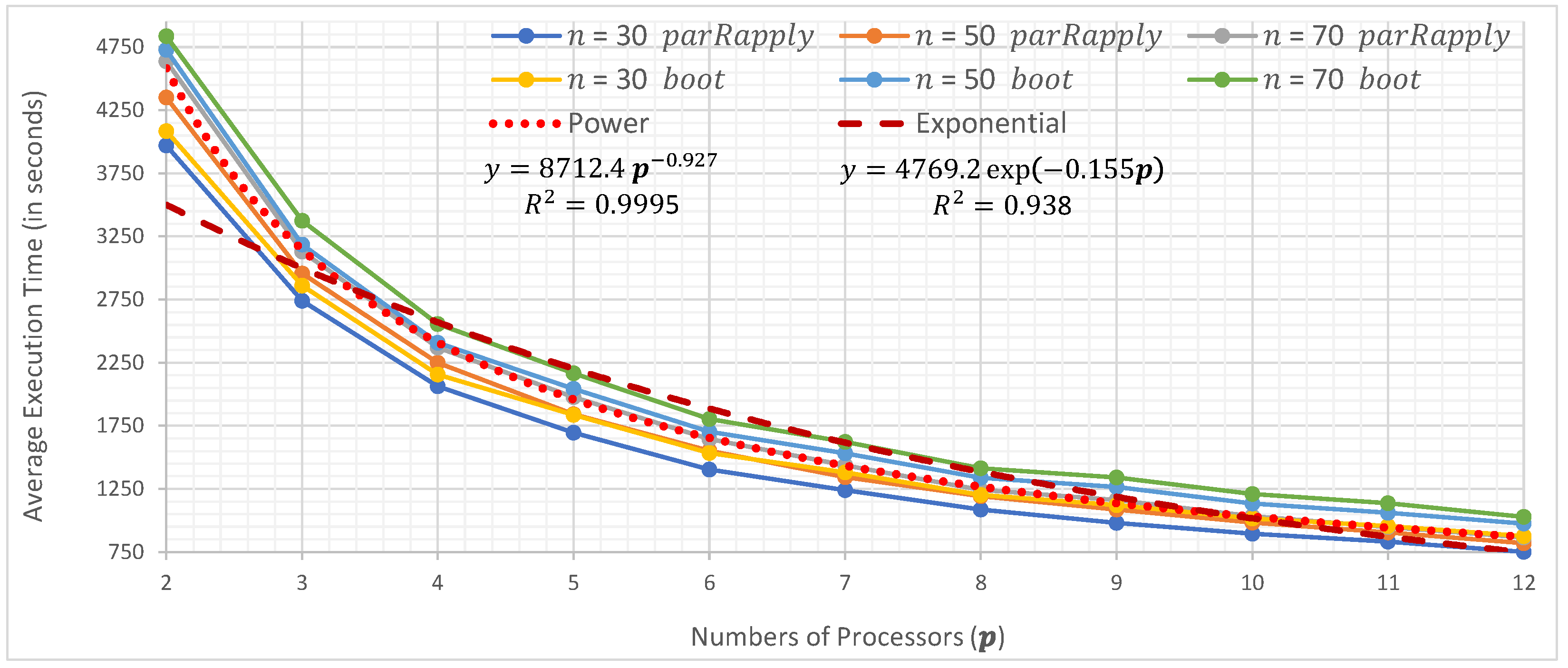
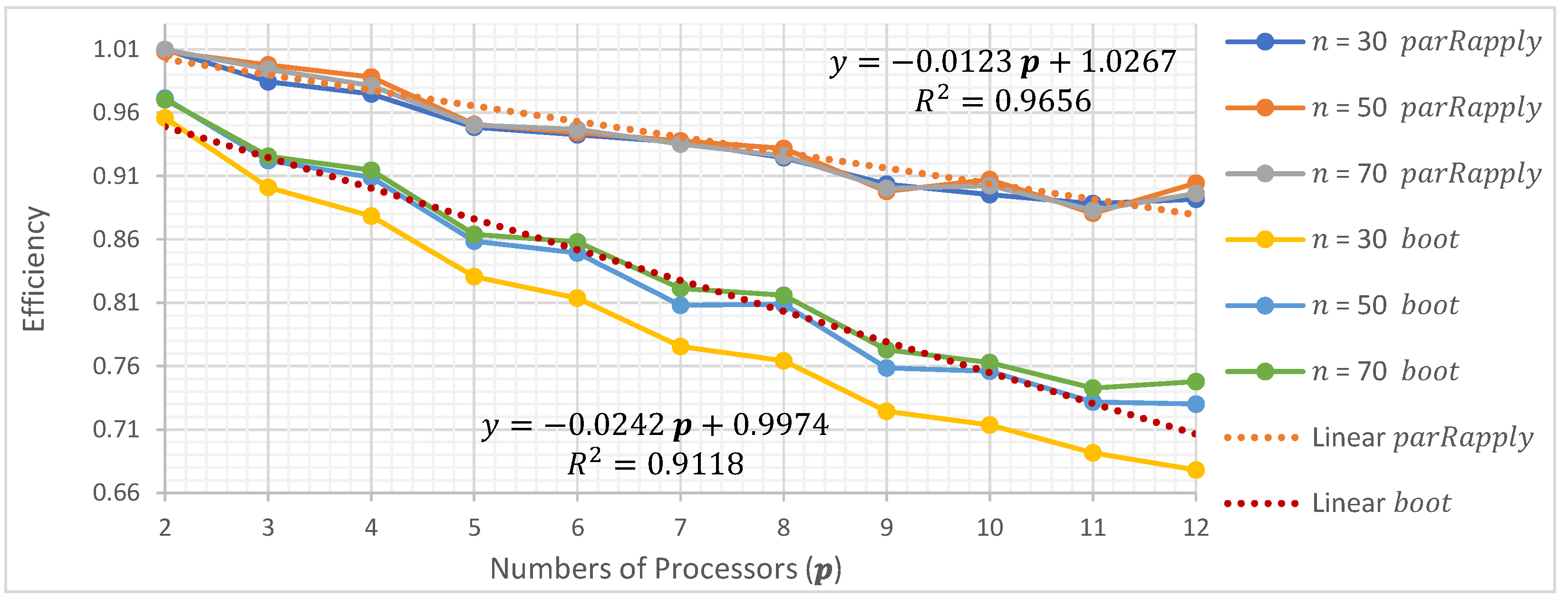
In this section, the average execution times are presented as a function of the number of processors used when running the two parallel implementations (parRapply and boot) analyzed in this research.
       
    
    Table A1.
    Average execution time (in seconds) using parRapply,  (1.5, 1, 0.31), weight vectors , sample size n, for different numbers of processors p.
  
Table A1.
    Average execution time (in seconds) using parRapply,  (1.5, 1, 0.31), weight vectors , sample size n, for different numbers of processors p.
      | n = 30 | n = 50 | n = 70 | |||||||||||
|---|---|---|---|---|---|---|---|---|---|---|---|---|---|
| p | |||||||||||||
| 2 | 4049 | 4058 | 4063 | 4088 | 4402 | 4428 | 4413 | 4440 | 4657 | 4662 | 4663 | 4,674 | |
| 3 | 2764 | 2762 | 2801 | 2793 | 2959 | 2979 | 2970 | 3006 | 3164 | 3142 | 3164 | 3162 | |
| 4 | 2118 | 2100 | 2092 | 2112 | 2261 | 2259 | 2255 | 2248 | 2406 | 2399 | 2389 | 2404 | |
| 5 | 1726 | 1761 | 1713 | 1724 | 1868 | 1888 | 1874 | 1870 | 2004 | 1970 | 1988 | 1,969 | |
| 6 | 1445 | 1457 | 1444 | 1461 | 1575 | 1551 | 1601 | 1567 | 1679 | 1658 | 1640 | 1655 | |
| 7 | 1242 | 1246 | 1257 | 1263 | 1365 | 1350 | 1361 | 1356 | 1432 | 1457 | 1420 | 1447 | |
| 8 | 1102 | 1125 | 1123 | 1090 | 1203 | 1193 | 1191 | 1196 | 1288 | 1261 | 1274 | 1264 | |
| 9 | 1007 | 1007 | 1012 | 1012 | 1105 | 1099 | 1112 | 1097 | 1158 | 1162 | 1160 | 1171 | |
| 10 | 919 | 916 | 914 | 918 | 988 | 981 | 976 | 986 | 1044 | 1039 | 1055 | 1037 | |
| 11 | 841 | 840 | 835 | 845 | 905 | 931 | 913 | 933 | 963 | 975 | 960 | 981 | |
| 12 | 764 | 765 | 764 | 776 | 823 | 820 | 820 | 823 | 869 | 875 | 882 | 877 | |
       
    
    Table A2.
    Average execution time (in seconds) using boot,  (1.5, 1, 0.31), weight vectors , sample size n, for different numbers of processors p.
  
Table A2.
    Average execution time (in seconds) using boot,  (1.5, 1, 0.31), weight vectors , sample size n, for different numbers of processors p.
      | n = 30 | n = 50 | n = 70 | |||||||||||
|---|---|---|---|---|---|---|---|---|---|---|---|---|---|
| p | |||||||||||||
| 2 | 4359 | 4377 | 4338 | 4351 | 4645 | 4660 | 4672 | 4650 | 4936 | 4943 | 4941 | 4,948 | |
| 3 | 3089 | 3078 | 3078 | 3079 | 3271 | 3280 | 3269 | 3258 | 3453 | 3454 | 3465 | 3,443 | |
| 4 | 2368 | 2368 | 2367 | 2380 | 2496 | 2489 | 2489 | 2478 | 2631 | 2626 | 2626 | 2605 | |
| 5 | 2003 | 2010 | 1998 | 2010 | 2110 | 2114 | 2098 | 2107 | 2229 | 2225 | 2219 | 2,209 | |
| 6 | 1701 | 1707 | 1710 | 1706 | 1775 | 1772 | 1783 | 1771 | 1875 | 1852 | 1861 | 1,863 | |
| 7 | 1543 | 1533 | 1532 | 1530 | 1598 | 1602 | 1600 | 1598 | 1670 | 1670 | 1666 | 1666 | |
| 8 | 1366 | 1360 | 1362 | 1362 | 1395 | 1400 | 1403 | 1393 | 1465 | 1471 | 1465 | 1476 | |
| 9 | 1280 | 1270 | 1281 | 1280 | 1322 | 1322 | 1328 | 1328 | 1376 | 1379 | 1377 | 1382 | |
| 10 | 1161 | 1177 | 1162 | 1169 | 1194 | 1193 | 1203 | 1196 | 1260 | 1255 | 1261 | 1254 | |
| 11 | 1098 | 1088 | 1095 | 1099 | 1126 | 1125 | 1119 | 1126 | 1173 | 1175 | 1170 | 1178 | |
| 12 | 1025 | 1020 | 1022 | 1027 | 1027 | 1029 | 1040 | 1034 | 1074 | 1072 | 1058 | 1071 | |
       
    
    Table A3.
    Average execution time (in seconds) using parRapply,  (1.5, 1, 0.62), weight vectors , sample size n, for different numbers of processors p.
  
Table A3.
    Average execution time (in seconds) using parRapply,  (1.5, 1, 0.62), weight vectors , sample size n, for different numbers of processors p.
      | n = 30 | n = 50 | n = 70 | |||||||||||
|---|---|---|---|---|---|---|---|---|---|---|---|---|---|
| p | |||||||||||||
| 2 | 3897 | 3879 | 3969 | 3890 | 4257 | 4316 | 4291 | 4261 | 4529 | 4544 | 4530 | 4,564 | |
| 3 | 2658 | 2632 | 2626 | 2646 | 2889 | 2886 | 2915 | 2909 | 3107 | 3109 | 3091 | 3,093 | |
| 4 | 2037 | 2011 | 2015 | 2005 | 2178 | 2208 | 2195 | 2186 | 2330 | 2322 | 2343 | 2,344 | |
| 5 | 1669 | 1638 | 1672 | 1673 | 1797 | 1819 | 1823 | 1809 | 1925 | 1934 | 1949 | 1,927 | |
| 6 | 1391 | 1392 | 1375 | 1392 | 1495 | 1514 | 1524 | 1516 | 1609 | 1610 | 1610 | 1,615 | |
| 7 | 1200 | 1195 | 1205 | 1201 | 1311 | 1307 | 1317 | 1326 | 1388 | 1396 | 1380 | 1399 | |
| 8 | 1064 | 1046 | 1053 | 1001 | 1149 | 1156 | 1149 | 1151 | 1218 | 1236 | 1212 | 1224 | |
| 9 | 974 | 976 | 970 | 970 | 1058 | 1066 | 1059 | 1071 | 1117 | 1135 | 1124 | 1131 | |
| 10 | 867 | 873 | 877 | 874 | 973 | 948 | 972 | 950 | 1021 | 1004 | 1016 | 1023 | |
| 11 | 819 | 806 | 807 | 815 | 873 | 886 | 876 | 886 | 929 | 959 | 959 | 948 | |
| 12 | 728 | 737 | 730 | 738 | 820 | 807 | 806 | 810 | 859 | 861 | 853 | 858 | |
       
    
    Table A4.
    Average execution time (in seconds) using boot,  (1.5, 1, 0.62), weight vectors , sample size n, for different numbers of processors p.
  
Table A4.
    Average execution time (in seconds) using boot,  (1.5, 1, 0.62), weight vectors , sample size n, for different numbers of processors p.
      | n = 30 | n = 50 | n = 70 | |||||||||||
|---|---|---|---|---|---|---|---|---|---|---|---|---|---|
| p | |||||||||||||
| 2 | 4133 | 4111 | 4110 | 4110 | 4542 | 4552 | 4529 | 4530 | 4840 | 4836 | 4844 | 4833 | |
| 3 | 2883 | 2874 | 2891 | 2875 | 3169 | 3175 | 3162 | 3160 | 3381 | 3372 | 3395 | 3373 | |
| 4 | 2184 | 2184 | 2188 | 2181 | 2394 | 2396 | 2388 | 2394 | 2549 | 2547 | 2564 | 2550 | |
| 5 | 1857 | 1854 | 1853 | 1854 | 2034 | 2031 | 2027 | 2033 | 2163 | 2155 | 2174 | 2158 | |
| 6 | 1555 | 1559 | 1554 | 1553 | 1697 | 1696 | 1697 | 1696 | 1810 | 1798 | 1810 | 1801 | |
| 7 | 1403 | 1397 | 1401 | 1399 | 1528 | 1526 | 1524 | 1525 | 1621 | 1619 | 1622 | 1622 | |
| 8 | 1223 | 1226 | 1223 | 1225 | 1335 | 1333 | 1335 | 1333 | 1420 | 1411 | 1419 | 1410 | |
| 9 | 1147 | 1144 | 1145 | 1145 | 1259 | 1258 | 1256 | 1256 | 1340 | 1338 | 1341 | 1,339 | |
| 10 | 1037 | 1036 | 1036 | 1037 | 1132 | 1131 | 1132 | 1132 | 1211 | 1208 | 1212 | 1209 | |
| 11 | 972 | 973 | 968 | 972 | 1058 | 1056 | 1055 | 1056 | 1133 | 1132 | 1133 | 1129 | |
| 12 | 892 | 893 | 895 | 898 | 973 | 971 | 962 | 973 | 1035 | 1024 | 1032 | 1024 | |
       
    
    Table A5.
    Average execution time (in seconds) using parRapply,  (1.5, 1, 0.92), weight vectors , sample size n, for different numbers of processors p.
  
Table A5.
    Average execution time (in seconds) using parRapply,  (1.5, 1, 0.92), weight vectors , sample size n, for different numbers of processors p.
      | n = 30 | n = 50 | n = 70 | |||||||||||
|---|---|---|---|---|---|---|---|---|---|---|---|---|---|
| p | |||||||||||||
| 2 | 3970 | 3971 | 4000 | 4004 | 4351 | 4331 | 4355 | 4326 | 4639 | 4619 | 4654 | 4599 | |
| 3 | 2740 | 2713 | 2701 | 2708 | 2956 | 2963 | 2969 | 2947 | 3130 | 3178 | 3106 | 3130 | |
| 4 | 2064 | 2049 | 2028 | 2042 | 2250 | 2251 | 2253 | 2251 | 2369 | 2391 | 2349 | 2354 | |
| 5 | 1696 | 1677 | 1668 | 1686 | 1841 | 1865 | 1855 | 1845 | 1978 | 1962 | 1959 | 1973 | |
| 6 | 1403 | 1411 | 1399 | 1438 | 1551 | 1549 | 1538 | 1537 | 1645 | 1630 | 1620 | 1617 | |
| 7 | 1239 | 1221 | 1235 | 1224 | 1344 | 1339 | 1329 | 1328 | 1436 | 1414 | 1419 | 1409 | |
| 8 | 1087 | 1059 | 1079 | 1076 | 1191 | 1172 | 1174 | 1192 | 1243 | 1238 | 1234 | 1234 | |
| 9 | 981 | 986 | 998 | 989 | 1086 | 1080 | 1083 | 1086 | 1162 | 1144 | 1139 | 1138 | |
| 10 | 896 | 881 | 886 | 882 | 983 | 975 | 972 | 989 | 1034 | 1037 | 1027 | 1030 | |
| 11 | 832 | 819 | 841 | 820 | 906 | 893 | 884 | 912 | 948 | 943 | 944 | 948 | |
| 12 | 751 | 742 | 753 | 751 | 820 | 823 | 825 | 823 | 866 | 868 | 873 | 871 | |
       
    
    Table A6.
    Average execution time (in seconds) using boot,  (1.5, 1, 0.92), weight vectors , sample size n, for different numbers of processors p.
  
Table A6.
    Average execution time (in seconds) using boot,  (1.5, 1, 0.92), weight vectors , sample size n, for different numbers of processors p.
      | n = 30 | n = 50 | n = 70 | |||||||||||
|---|---|---|---|---|---|---|---|---|---|---|---|---|---|
| p | |||||||||||||
| 2 | 4085 | 4083 | 4083 | 4082 | 4728 | 4551 | 4539 | 4535 | 4836 | 4839 | 4839 | 4830 | |
| 3 | 2860 | 2850 | 2847 | 2856 | 3185 | 3175 | 3165 | 3166 | 3374 | 3372 | 3396 | 3376 | |
| 4 | 2155 | 2159 | 2169 | 2155 | 2407 | 2396 | 2391 | 2401 | 2556 | 2543 | 2547 | 2547 | |
| 5 | 1836 | 1838 | 1837 | 1835 | 2044 | 2034 | 2032 | 2035 | 2166 | 2156 | 2164 | 2164 | |
| 6 | 1534 | 1530 | 1536 | 1527 | 1704 | 1700 | 1698 | 1698 | 1804 | 1806 | 1808 | 1,811 | |
| 7 | 1381 | 1382 | 1380 | 1381 | 1533 | 1531 | 1526 | 1528 | 1622 | 1622 | 1625 | 1,626 | |
| 8 | 1202 | 1203 | 1203 | 1206 | 1339 | 1337 | 1333 | 1333 | 1414 | 1417 | 1418 | 1413 | |
| 9 | 1121 | 1125 | 1122 | 1126 | 1264 | 1264 | 1262 | 1260 | 1341 | 1341 | 1342 | 1339 | |
| 10 | 1016 | 1018 | 1018 | 1018 | 1133 | 1132 | 1133 | 1135 | 1210 | 1210 | 1214 | 1208 | |
| 11 | 956 | 955 | 955 | 954 | 1060 | 1059 | 1058 | 1058 | 1136 | 1134 | 1135 | 1134 | |
| 12 | 876 | 881 | 886 | 877 | 975 | 976 | 965 | 966 | 1028 | 1028 | 1027 | 1027 | |
       
    
    Table A7.
    Average execution time (in seconds) using parRapply,  (1, 1, 0.5), weight vectors , sample size n, for different numbers of processors p.
  
Table A7.
    Average execution time (in seconds) using parRapply,  (1, 1, 0.5), weight vectors , sample size n, for different numbers of processors p.
      | n = 30 | n = 50 | n = 70 | |||||||||||
|---|---|---|---|---|---|---|---|---|---|---|---|---|---|
| p | |||||||||||||
| 2 | 3457 | 3439 | 3509 | 3475 | 3727 | 3759 | 3767 | 3771 | 3960 | 3978 | 3952 | 3979 | |
| 3 | 2341 | 2330 | 2326 | 2350 | 2498 | 2522 | 2539 | 2517 | 2679 | 2721 | 2676 | 2704 | |
| 4 | 1782 | 1769 | 1769 | 1758 | 1929 | 1931 | 1914 | 1930 | 2053 | 2037 | 2031 | 2034 | |
| 5 | 1466 | 1479 | 1468 | 1491 | 1591 | 1595 | 1602 | 1590 | 1679 | 1673 | 1690 | 1680 | |
| 6 | 1222 | 1228 | 1222 | 1232 | 1326 | 1335 | 1325 | 1329 | 1415 | 1399 | 1413 | 1409 | |
| 7 | 1070 | 1075 | 1063 | 1061 | 1150 | 1156 | 1138 | 1146 | 1229 | 1211 | 1210 | 1213 | |
| 8 | 941 | 938 | 942 | 931 | 1003 | 1004 | 1015 | 1013 | 1075 | 1070 | 1072 | 1074 | |
| 9 | 848 | 849 | 849 | 858 | 936 | 924 | 923 | 930 | 976 | 1011 | 987 | 1016 | |
| 10 | 777 | 808 | 781 | 774 | 839 | 834 | 835 | 839 | 888 | 877 | 877 | 899 | |
| 11 | 715 | 703 | 725 | 723 | 773 | 768 | 773 | 774 | 813 | 821 | 823 | 823 | |
| 12 | 656 | 654 | 655 | 660 | 709 | 706 | 710 | 712 | 755 | 761 | 743 | 749 | |
       
    
    Table A8.
    Average execution time (in seconds) using boot,  (1, 1, 0.5), weight vectors , sample size n, for different numbers of processors p.
  
Table A8.
    Average execution time (in seconds) using boot,  (1, 1, 0.5), weight vectors , sample size n, for different numbers of processors p.
      | n = 30 | n = 50 | n = 70 | |||||||||||
|---|---|---|---|---|---|---|---|---|---|---|---|---|---|
| p | |||||||||||||
| 2 | 3665 | 3673 | 3670 | 3682 | 4000 | 3983 | 3988 | 3992 | 4249 | 4255 | 4238 | 4241 | |
| 3 | 2577 | 2572 | 2589 | 2586 | 2792 | 2786 | 2799 | 2806 | 2971 | 2984 | 2966 | 2967 | |
| 4 | 1955 | 1947 | 1959 | 1961 | 2109 | 2103 | 2113 | 2110 | 2233 | 2247 | 2229 | 2235 | |
| 5 | 1668 | 1663 | 1662 | 1667 | 1794 | 1790 | 1797 | 1795 | 1901 | 1908 | 1898 | 1903 | |
| 6 | 1399 | 1400 | 1394 | 1399 | 1497 | 1498 | 1497 | 1498 | 1584 | 1591 | 1590 | 1594 | |
| 7 | 1263 | 1260 | 1262 | 1256 | 1351 | 1353 | 1355 | 1352 | 1431 | 1432 | 1431 | 1433 | |
| 8 | 1091 | 1092 | 1093 | 1092 | 1175 | 1170 | 1172 | 1174 | 1254 | 1250 | 1250 | 1252 | |
| 9 | 1014 | 1014 | 1019 | 1015 | 1093 | 1091 | 1095 | 1095 | 1172 | 1172 | 1175 | 1169 | |
| 10 | 938 | 935 | 933 | 932 | 989 | 989 | 988 | 989 | 1049 | 1048 | 1052 | 1050 | |
| 11 | 875 | 878 | 880 | 877 | 931 | 929 | 929 | 930 | 985 | 986 | 988 | 986 | |
| 12 | 809 | 810 | 809 | 810 | 859 | 862 | 861 | 860 | 904 | 904 | 913 | 911 | |
       
    
    Table A9.
    Average execution time (in seconds) using parRapply,  (1, 1, 0.25), weight vectors , sample size n, for different numbers of processors p.
  
Table A9.
    Average execution time (in seconds) using parRapply,  (1, 1, 0.25), weight vectors , sample size n, for different numbers of processors p.
      | n = 30 | n = 50 | n = 70 | |||||||||||
|---|---|---|---|---|---|---|---|---|---|---|---|---|---|
| p | |||||||||||||
| 2 | 3589 | 3605 | 3583 | 3587 | 3925 | 3975 | 3867 | 3904 | 4113 | 4063 | 4154 | 4105 | |
| 3 | 2436 | 2452 | 2442 | 2458 | 2660 | 2628 | 2630 | 2667 | 2792 | 2837 | 2796 | 2803 | |
| 4 | 1844 | 1851 | 1859 | 1879 | 1998 | 1991 | 2018 | 1993 | 2105 | 2103 | 2139 | 2106 | |
| 5 | 1528 | 1563 | 1545 | 1537 | 1667 | 1669 | 1652 | 1648 | 1760 | 1762 | 1748 | 1745 | |
| 6 | 1280 | 1296 | 1277 | 1289 | 1375 | 1384 | 1382 | 1379 | 1445 | 1468 | 1449 | 1465 | |
| 7 | 1125 | 1114 | 1111 | 1136 | 1200 | 1194 | 1203 | 1223 | 1260 | 1267 | 1253 | 1260 | |
| 8 | 988 | 972 | 980 | 974 | 1062 | 1043 | 1049 | 1059 | 1108 | 1100 | 1109 | 1111 | |
| 9 | 890 | 892 | 897 | 892 | 960 | 957 | 968 | 958 | 1054 | 1014 | 1038 | 1017 | |
| 10 | 811 | 812 | 810 | 799 | 874 | 880 | 870 | 872 | 914 | 925 | 910 | 921 | |
| 11 | 748 | 746 | 751 | 742 | 797 | 821 | 799 | 794 | 846 | 850 | 855 | 846 | |
| 12 | 689 | 678 | 687 | 685 | 745 | 736 | 738 | 739 | 771 | 786 | 773 | 779 | |
       
    
    Table A10.
    Average execution time (in seconds) using boot,  (1, 1, 0.25), weight vectors , sample size n, for different numbers of processors p.
  
Table A10.
    Average execution time (in seconds) using boot,  (1, 1, 0.25), weight vectors , sample size n, for different numbers of processors p.
      | n = 30 | n = 50 | n = 70 | |||||||||||
|---|---|---|---|---|---|---|---|---|---|---|---|---|---|
| p | |||||||||||||
| 2 | 3968 | 3950 | 3972 | 3954 | 4136 | 4150 | 4142 | 4141 | 4368 | 4354 | 4384 | 4386 | |
| 3 | 2830 | 2809 | 2812 | 2813 | 2923 | 2913 | 2922 | 2907 | 3069 | 3086 | 3058 | 3065 | |
| 4 | 2175 | 2166 | 2169 | 2164 | 2215 | 2222 | 2229 | 2222 | 2319 | 2328 | 2333 | 2323 | |
| 5 | 1848 | 1845 | 1853 | 1856 | 1892 | 1892 | 1893 | 1888 | 1972 | 1980 | 1972 | 1972 | |
| 6 | 1586 | 1570 | 1570 | 1580 | 1590 | 1590 | 1595 | 1586 | 1663 | 1659 | 1651 | 1664 | |
| 7 | 1416 | 1421 | 1419 | 1424 | 1430 | 1438 | 1443 | 1434 | 1487 | 1484 | 1480 | 1483 | |
| 8 | 1255 | 1251 | 1252 | 1256 | 1255 | 1261 | 1260 | 1255 | 1303 | 1299 | 1302 | 1310 | |
| 9 | 1171 | 1180 | 1181 | 1178 | 1169 | 1174 | 1176 | 1176 | 1222 | 1224 | 1226 | 1219 | |
| 10 | 1082 | 1086 | 1087 | 1084 | 1069 | 1070 | 1068 | 1074 | 1100 | 1096 | 1099 | 1102 | |
| 11 | 1028 | 1020 | 1019 | 1025 | 1003 | 1008 | 1007 | 1002 | 1028 | 1031 | 1032 | 1027 | |
| 12 | 954 | 952 | 959 | 952 | 931 | 935 | 925 | 927 | 950 | 952 | 946 | 953 | |
       
    
    Table A11.
    Average execution time (in seconds) using parRapply,  (1, 1, 0.75), weight vectors , sample size n, for different numbers of processors p.
  
Table A11.
    Average execution time (in seconds) using parRapply,  (1, 1, 0.75), weight vectors , sample size n, for different numbers of processors p.
      | n = 30 | n = 50 | n = 70 | |||||||||||
|---|---|---|---|---|---|---|---|---|---|---|---|---|---|
| p | |||||||||||||
| 2 | 3383 | 3426 | 3400 | 3418 | 3731 | 3716 | 3725 | 3733 | 3946 | 3970 | 3981 | 3963 | |
| 3 | 2321 | 2293 | 2321 | 2296 | 2511 | 2543 | 2525 | 2566 | 2697 | 2690 | 2705 | 2683 | |
| 4 | 1742 | 1755 | 1752 | 1747 | 1899 | 1910 | 1931 | 1918 | 2064 | 2021 | 2031 | 2063 | |
| 5 | 1478 | 1451 | 1462 | 1444 | 1610 | 1585 | 1599 | 1603 | 1701 | 1693 | 1702 | 1700 | |
| 6 | 1204 | 1205 | 1214 | 1217 | 1320 | 1315 | 1338 | 1322 | 1410 | 1405 | 1416 | 1408 | |
| 7 | 1053 | 1040 | 1036 | 1047 | 1150 | 1146 | 1145 | 1147 | 1238 | 1234 | 1225 | 1227 | |
| 8 | 907 | 927 | 916 | 927 | 1002 | 1009 | 1009 | 1004 | 1077 | 1083 | 1090 | 1062 | |
| 9 | 850 | 844 | 847 | 852 | 931 | 921 | 920 | 920 | 974 | 988 | 978 | 992 | |
| 10 | 755 | 767 | 762 | 767 | 831 | 831 | 843 | 842 | 892 | 897 | 894 | 885 | |
| 11 | 701 | 708 | 713 | 699 | 775 | 762 | 770 | 772 | 810 | 801 | 805 | 812 | |
| 12 | 643 | 647 | 648 | 645 | 711 | 713 | 700 | 707 | 759 | 750 | 759 | 753 | |
       
    
    Table A12.
    Average execution time (in seconds) using boot,  (1, 1, 0.75), weight vectors , sample size n, for different numbers of processors p.
  
Table A12.
    Average execution time (in seconds) using boot,  (1, 1, 0.75), weight vectors , sample size n, for different numbers of processors p.
      | n = 30 | n = 50 | n = 70 | |||||||||||
|---|---|---|---|---|---|---|---|---|---|---|---|---|---|
| p | |||||||||||||
| 2 | 3582 | 3601 | 3601 | 3596 | 3957 | 3978 | 3983 | 3966 | 4226 | 4631 | 4244 | 4254 | |
| 3 | 2533 | 2524 | 2539 | 2532 | 2789 | 2790 | 2795 | 2783 | 2963 | 2957 | 2966 | 2972 | |
| 4 | 1904 | 1900 | 1905 | 1900 | 2105 | 2099 | 2095 | 2088 | 2228 | 2335 | 2229 | 2241 | |
| 5 | 1625 | 1623 | 1621 | 1622 | 1791 | 1791 | 1789 | 1785 | 1901 | 1904 | 1898 | 1897 | |
| 6 | 1358 | 1356 | 1353 | 1351 | 1486 | 1492 | 1491 | 1484 | 1588 | 1589 | 1585 | 1585 | |
| 7 | 1220 | 1219 | 1218 | 1218 | 1346 | 1347 | 1345 | 1347 | 1428 | 1432 | 1427 | 1427 | |
| 8 | 1053 | 1050 | 1049 | 1052 | 1169 | 1166 | 1166 | 1161 | 1245 | 1249 | 1249 | 1247 | |
| 9 | 976 | 978 | 978 | 979 | 1086 | 1087 | 1087 | 1084 | 1169 | 1170 | 1170 | 1169 | |
| 10 | 895 | 895 | 894 | 896 | 983 | 984 | 985 | 982 | 1048 | 1050 | 1049 | 1051 | |
| 11 | 843 | 844 | 843 | 846 | 927 | 925 | 925 | 924 | 984 | 986 | 986 | 985 | |
| 12 | 782 | 777 | 775 | 784 | 856 | 849 | 860 | 857 | 903 | 911 | 914 | 906 | |
References
- Novoa-Muñoz, F.; Jiménez-Gamero, M.D. Testing for the bivariate Poisson distribution. Metrika 2014, 77, 771–793. [Google Scholar] [CrossRef]
 - Bolis, A.; Cantwell, C.D.; Moxey, D.; Serson, D.; Sherwin, S.J. An adaptable parallel algorithm for the direct numerical simulation of incompressible turbulent flows using a Fourier spectral/hp element method and MPI virtual topologies. Comput. Phys. Commun. 2016, 206, 17–25. [Google Scholar] [CrossRef] [PubMed]
 - Macías-Díaz, J.E. An easy-to-implement parallel algorithm to simulate complex instabilities in three-dimensional (fractional) hyperbolic systems. Comput. Phys. Commun. 2020, 254, 51059. [Google Scholar] [CrossRef]
 - Laman, D.S.; Wieringen, W.N. A parallel algorithm for ridge-penalized estimation of the multivariate exponential family from data of mixed types. Stat. Comput. 2021, 31, 41. [Google Scholar] [CrossRef]
 - Yang, D.; Li, M.; Liu, H. A Parallel Computing Algorithm for the Emergency-Oriented Atmospheric Dispersion Model CALPUFF. Atmosphere 2022, 13, 2129. [Google Scholar] [CrossRef]
 - Trabes, G.; Wainer, G.; Gil-Costa, V. A Parallel Algorithm to Accelerate DEVS Simulations in Shared Memory Architectures. IEEE Trans. Parallel Distrib. Syst. 2023, 34, 1609–1620. [Google Scholar] [CrossRef]
 - Wu, X.; Kolar, A.; Chung, J.; Jin, D.; Suchara, M.; Kettimuthu, R. Parallel Simulation of Quantum Networks with Distributed Quantum State Management. ACM Trans. Model. Comput. 2024, 34, 1–28. [Google Scholar] [CrossRef]
 - Kocherlakota, S.; Kocherlakota, K. Bivariate Discrete Distributions; CRC Press: Boca Raton, FL, USA, 2017. [Google Scholar]
 - Rohatgi, V.K.; Saleh, A.K.M.E. An Introduction to Probability Theory and Mathematical Statistics, 3rd ed.; Wiley Series in Probability and Statistics; John Wiley & Sons: Hoboken, NJ, USA, 2015. [Google Scholar]
 - Shao, J. Mathematical Statistics; Springer Science & Business Media: New York, NY, USA, 2008. [Google Scholar]
 - Andrew, D. Inconsistency of the bootstrap when a parameter is on the boundary of the parameter space. Econométrica 2000, 68, 399–400. [Google Scholar] [CrossRef]
 - Pacheco, P. An Introduction to Parallel Programming; Morgan Kaufmann Publishers: Burlington, MA, USA, 2011. [Google Scholar]
 - R Core Team. R: A Language and Environment for Statistical Computing; R Foundation for Statistical Computing, Vienna, Austria. 2020. Available online: https://www.R-project.org/ (accessed on 5 June 2021).
 - Urbanek, S. Multicore: Parallel Processing of R Code on Machines with Multiple Cores or CPUs; 2014. Available online: https://cran.r-project.org/package=multicore (accessed on 25 July 2021).
 - Canty, A.; Ripley, B.D.; boot: Bootstrap R (S-Plus) Functions. R Package Version 1.3-30; 2024. Available online: https://cran.r-project.org/web/packages/boot/boot.pdf (accessed on 12 May 2024).
 - Chapple, S.; Eilidh, T.; Thorsten, F.; Terence, S. Mastering Parallel Programming with R; Packt Publishing Ltd.: Birmingham, UK, 2016. [Google Scholar]
 - Matloff, N. Parallel Computing for Data Science; Chapman and Hall/CRC: New York, NY, USA, 2016. [Google Scholar]
 - Rauber, T.; Rünger, G. Parallel Programming, 3rd ed.; Springer: Cham, Switzerland, 2023. [Google Scholar]
 - Novoa-Muñoz, F.; Jiménez-Gamero, M.D. A goodness-of-fit test for the multivariate Poisson distribution. SORT 2016, 40, 113–138. [Google Scholar]
 - Novoa-Muñoz, F. Goodness-of-fit tests for the bivariate Poisson distribution. Commun. Stat. Simul. Comput. 2021, 50, 1998–2014. [Google Scholar] [CrossRef]
 - González-Albornoz, P.; Novoa-Muñoz, F. Goodness-of-Fit Test for the Bivariate Hermite Distribution. Axioms 2023, 12, 7. [Google Scholar] [CrossRef]
 
Disclaimer/Publisher’s Note: The statements, opinions and data contained in all publications are solely those of the individual author(s) and contributor(s) and not of MDPI and/or the editor(s). MDPI and/or the editor(s) disclaim responsibility for any injury to people or property resulting from any ideas, methods, instructions or products referred to in the content.  | 
© 2024 by the author. Licensee MDPI, Basel, Switzerland. This article is an open access article distributed under the terms and conditions of the Creative Commons Attribution (CC BY) license (https://creativecommons.org/licenses/by/4.0/).