Sparse Clustering Algorithm Based on Multi-Domain Dimensionality Reduction Autoencoder

Abstract

The key to high-dimensional clustering lies in discovering the intrinsic structures and patterns in data to provide valuable information. However, high-dimensional clustering faces enormous challenges such as dimensionality disaster, increased data sparsity, and reduced reliability of the clustering results. In order to address these issues, we propose a sparse clustering algorithm based on a multi-domain dimensionality reduction model. This method achieves high-dimensional clustering by integrating the sparse reconstruction process and sparse L1 regularization into a deep autoencoder model. A sparse reconstruction module is designed based on the L1 sparse reconstruction of features under different domains to reconstruct the data. The proposed method mainly contributes in two aspects. Firstly, the spatial and frequency domains are combined by taking into account the spatial distribution and frequency characteristics of the data to provide multiple perspectives and choices for data analysis and processing. Then, a neural network-based clustering model with sparsity is conducted by projecting data points onto multi-domains and implementing adaptive regularization penalty terms to the weight matrix. The experimental results demonstrate superior performance of the proposed method in handling clustering problems on high-dimensional datasets.

1. Introduction

Clustering is one of the fundamental topics in machine learning to explore correlations within data by partitioning a set of samples into a number of homogeneous clusters [1]. It is intensively applied to security, text mining, image processing, bioinformatics and other fields [2]. Under the situation of no prior knowledge or a small amount of prior knowledge, clustering models usually classify data according to the similarity or dissimilarity measure between data, where the aim is to make intra-class data tend to be highly similar while inter-class data tend to be highly different [3]. To discover useful information hidden in a large amount of data, it helps to divide the data into several different groups with similar features. There is currently a large amount of research on clustering, such as centroid-based clustering, hierarchical clustering, and spectral clustering, to provide better understanding of the structure and discovers patterns and trends in the data. However, clustering on high-dimensional data remains a challenging research topic.

High-dimensional data are widely used in fields such as computer vision. Compared to low-dimensional data, high-dimensional data can provide richer information, help to gain a deeper understanding of the data and discover hidden complex relationships, leading to more accurate predictions. However, in high-dimensional data, there is often a large amount of redundant information, which poses great challenges to data processing and even leads to the problem of the “curse of dimensionality”. This also makes a predicament in clustering analysis, causing the failure of traditional clustering methods in dealing with high-dimensional data. As the dimensionality of data increases, the difficulty of clustering also increases. Therefore, continuing to explore new methods of high-dimensional clustering to address the challenges of big data is of great significance.

The high-dimensional clustering mainly confronts the following challenges:

• As the dimension of data increases, a large number of irrelevant attributes emerge in high-dimensional datasets, which cannot form obvious data clusters in all dimensions. In high-dimensional space, the distribution of data points becomes sparser, and it is hard to find the correct clustering structure. Different distance measurement methods may generate different clustering results.
• In high-dimensional data, data points becomes increasingly similar and the distance between them becomes more blurred. In this situation, traditional clustering methods often fail to fully capture the intrinsic structure of data, making it difficult to effectively identify and distinguish different data categories.

To address these problems, researchers have proposed various methods including ensemble clustering clustering, subspace clustering, and dimensionality reduction-based clustering. Huang et al. [4] introduced a new multi-directional integrated clustering method to solve the curse of dimensionality in high-dimensional data by creating a large number of diverse metrics and utilizing consistency functions to explore clustering diversity. Jia et al. [5] proposed a unified numerical and classification attribute weighting scheme based on subspace clustering, which quantifies the contribution of attributes to clustering by considering inter-cluster differences and intra-cluster similarity, thereby improving the processing ability of high-dimensional data. Hou et al. [6] proposed a new framework called discriminative embedding clustering, which iteratively alternates dimensionality reduction and clustering to improve the ability to efficiently process and manage large-scale high-dimensional data.

Clustering algorithms such as k-means and hierarchical clustering typically rely on manually designed features or similarity measures, which is limited when dealing with complex high-dimensional data. In recent years, deep learning has been used to improve clustering performance significantly. It can discover intricate patterns in data by learning feature representations and improve clustering performance. In 2022, Peng et al. [7] directly established interpretable neural layers to achieve end-to-end clustering learning. Inspired by this, we propose a sparse clustering model based on a multi-domain dimensionality reduction architecture (SMDR). Furthermore, the proposed model accounts for features within both the frequency domain and spatial domain information to facilitate a more comprehensive data analysis and foster improvements in clustering efficiency. On the one hand, the spatial part directly extracts features from data to obtain intrinsic law with intuitive characteristics of the high-dimensional data. On the other hand, frequency features mirror the contributions of each frequency component through decomposing data into different frequency components to capture more refined and complex information in high-dimensional data.

Our contributions of this work are summarized as follows:

• We present a sparse learning-based architecture with adaptive regularization to achieve clustering in high-dimensional data. An automatic encoder model is designed to generate sparsity in weights and reduce the complexity of clustering based on the multi-domain dimensionality reduction.
• The spatial information and frequency characteristics of data are combined to learn domain-invariant feature representation. This combination improves noise resistance, extracts rich features, achieves dimensionality reduction and compression, and provides more information and choices for data analysis and processing.

Compared with the TELL model [7], the proposed method amalgamates insights from both spatial and frequency domains to enhance clustering accuracy and robustness. This integration aims to mitigate inaccuracies and incompleteness in clustering outcomes, thereby facilitating a more nuanced description and analysis of data. SMDR enhances sparsity by introducing an adaptive regularization penalty term in the weight matrix to learn domain-invariant feature representation from both the spatial and frequency domains.

The remainder of the paper is organized as follows. Section 2 briefly introduces the related works for high-dimensional clustering. In Section 3, we detail the SDMR framework. Section 4 reports the experimental results on three benchmark datasets. Section 5 concludes the paper.

2. Related Work

High-dimensional clustering is one of the hot research topics that have attracted much attention in the past few years. A number of methods have been developed in traditional clustering and deep learning to realize clustering for high-dimensional data.

2.1. Clustering for High-Dimensional Data

High-dimensional data clustering usually suffers from the problem of data space sparsity. To address this issue, Jing et al. [8] extended the k-means clustering to process the weight of each dimension in each cluster and identify the subsets of important dimensions. Castelli et al. [9] proposed a singular value decomposition clustering such that the performance of nearest neighbor queries decreases with the increase in the number of dimensions. It groups homogeneous points into clusters and uses singular value decomposition to reduce the dimension of each cluster separately. To reduce the computational cost of the k-nearest neighbor method, Almalawi et al. [10] proposed a novel k-nearest neighbor method based on various width clustering. It first employs the global width for clustering, and then makes use of suitable local width recursive clustering. Ordonez et al. [11] proposed an effective disk-based k-means clustering to realize the effective clustering of data only by scanning the dataset a limited number of times. Rathore et al. [12] proposed FensiVAT clustering for large-scale high-dimensional data by leveraging dimensionality reduction and intelligent sampling strategies. To address the issue of requirement to preset the number of clusters for most clustering algorithms, Guan et al. [13] proposed a Density Mountains Separation (DEMOS) clustering algorithm. DEMOS determines the number of clusters by pruning density peaks within a density-boosting cluster tree. To solve the problem that the intrinsic structure of the data is destroyed, Zhao et al. [14] proposed a new fuzzy k-means clustering model for performing clustering tasks on flexible manifolds. The model is based on the fuzzy clustering of contraction patterns with the desired manifold structure.

2.2. Deep Learning Method

In recent years, deep learning has been widely used in clustering. Yang et al. [15] proposed an end-to-end deep multi-view clustering model with collaborative learning to predict the clustering results. Xu et al. [16] proposed a self-supervised discriminative feature learning for deep multi-view clustering. To better apply spectral clustering in unsupervised learning, Zhao et al. [17] introduced a deep learning framework with fully connected layers for learning a mapping function, replacing the traditional Laplacian matrix eigenvalue decomposition. Existing text-clustering algorithms suffer from high-dimensional and sparsity problems, and ignore text structure information. To meet these challenges, Guan et al. [18] proposed a deep feature-based clustering method to incorporate pre-trained text encoders into the text-clustering task. Clustering methods based on deep learning usually have the shortcomings of high complexity and requirements. Li et al. [19] proposed a self-supervised self-organizing clustering network to jointly learn feature extraction and feature clustering, thereby achieving a single-stage clustering method. Huang et al. [20] proposed a novel end-to-end deep clustering method with prototype scattering and forward sampling functions to make full use of both the contrast and non-contrast processes. Wang et al. [21] proposed a deep non-parametric Bayesian method to avoid the demand of knowing the number of clusters in traditional clustering methods and applied it to dual unsupervised joint learning of image clustering. To solve the problem that global clustering loss destroys the local geometry of the underlying data, Wang et al. [22] proposed a local to global deep clustering method based on approximately uniform manifolds in a two-stage manner. To combine representation learning and clustering, Chang et al. [23] reconsidered the definition of clustering tasks and developed a deep self-evolving clustering to jointly learn representations and cluster data. The encoder–decoder architecture limits the depth of the encoder, which severely reduces the ability to learn. To solve this problem, Ji et al. [24] proposed a decoderless variational deep embedding for clustering. To address the limitations of intrinsic linear and fixed structures, Li et al. [25] developed an adaptive deep clustering method to embed structured graph learning with adaptive neighbors into deep autoencoder networks. Deep generation model-based clustering methods have received a lot of attention due to their ability to learn promising potential embeddings from raw data. Yang et al. [26] proposed a novel clustering method based on a variational autoencoder with spherical latent embedding. Wu et al. [27] proposed a novel approach based on neural networks to achieve two related tasks and resolve their differences in an end-to-end manner. Wu et al. [28] combined subspace clustering with deep semi-supervised feature learning to face the challenge that the number of marker data for feature learning in deep neural networks is limited. In terms of learning adaptive sparse regularizers from a given input data for a specific task study, Wang et al. [29] proposed a deep sparse regularizer learning model that adaptively learns data-driven sparse regularizers. Peng et al. [7] developed the TELL model, which implements discrete k-means into a differentiable neural network with inherent interpretability and transparency. In TELL, an interpretable plug-and-play neural module is proposed as a differentiable alternative to the vanilla k-means for spatial clustering. It demonstrates significant advantages in interpretability and clustering performance and is one of the few explainable artificial intelligence studies focusing on unsupervised learning and data clustering.

Some clustering methods are based on learning domain-invariant representation. Lin et al. [30] proposed an efficient cross-clustering classification algorithm on non-geometric attributes of spatial clustering. It combines the information of two domains, iterating the clustering algorithm on the optimization domain and iterating the classification algorithm on the constrained domain, to effectively achieve the target clustering. Werner [31] proposed a multi-domain autoencoder model, abbreviated as MD autoencoder, for multi-domain research. In this paper, we propose a sparse clustering algorithm based on multi-domain dimensionality reduction model. By integrating sparse reconstruction process and sparse L1 regularization into the autoencoder model, the method can perform effective dimensionality reduction and clustering on the given high-dimensional data.

3. Sparse Clustering Algorithm Based on Multi-Domain Dimensionality Reduction Autoencoder

3.1. Multi-Domain Autoencoder

In this paper, we aim to achieve high-dimensional clustering in an end-to-end model. The sample data are encoded and mapped to a low-dimensional representation space from two domains. A multi-domain joint loss function is designed to guide the model to capture valuable information for clustering. The cluster loss part measures the importance of features between each cluster and the reconstruct loss part measures the reconstruction ability of data. The regulation term is used to inspire sparsity.

In its spatial form, the loss function is:

$$\begin{array}{ccc}{L}_{clu}^{\left(1\right)}\left(W^{\left(1\right)}\right)\hfill & =\hfill & {\displaystyle \sum _{n=1}^N}{\displaystyle \sum _{u=1}^U}\left({\mathcal{L}}_u\left(X_n^{\left(1\right)};W\right){\parallel X_n^{\left(1\right)}-x_u^{\left(1\right)}\left(W^{\left(1\right)}\right)\parallel }_2^2\right)\hfill \\ {\widehat{X}}_n^{\left(1\right)}\left(W^{\left(1\right)}\right)\hfill & =\hfill & g_{W^{\left(1\right)}}\left(f_{W^{\left(1\right)}}\left(X_n^{\left(1\right)}\right)\right)\hfill \\ L_{rec}^{\left(1\right)}\left(W^{\left(1\right)}\right)\hfill & =\hfill & {\displaystyle \sum _{n=1}^N}{\parallel X_n^{\left(1\right)}-{\widehat{X}}_n^{\left(1\right)}\left(W^{\left(1\right)}\right)\parallel }_2^2\hfill \\ L^{\left(1\right)}\left(W^{\left(1\right)}\right)\hfill & =\hfill & \lambda L_{clu}^{\left(1\right)}\left(W^{\left(1\right)}\right)+L_{rec}^{\left(1\right)}\left(W^{\left(1\right)}\right)\hfill \end{array}$$

(1)

where $W^{\left(1\right)}$ is the weight matrix of the clustering layer, $L_{clu}^{\left(1\right)}\left(W^{\left(1\right)}\right)$ is the clustering loss in the spatial domain, n is the index of the sample data, N is the number of sample data, u is the index of clusters, U is the number of clusters, ${\mathcal{L}}_u\left(X_n^{\left(1\right)};W^{\left(1\right)}\right)$ is the attention of the sample data in the uth spatial domain in the uth cluster, $X_n^{\left(1\right)}$ is the sample data, $x_u^{\left(1\right)}\left(W^{\left(1\right)}\right)$ is the clustering center of the uth cluster, ${\widehat{X}}_n^{\left(1\right)}\left(W^{\left(1\right)}\right)$ represents the reconstructed sample data, $f_{W^{\left(1\right)}}\left(·\right)$ represents the encoder, $g_{W^{\left(1\right)}}\left(·\right)$ represents the decoder, $L_{rec}^{\left(1\right)}\left(W^{\left(1\right)}\right)$ represents the reconstruction loss in the spatial domain, $\lambda =0.01$ weights the two losses, and $L^{\left(1\right)}\left(W^{\left(1\right)}\right)$ represents the total loss in the spatial domain.

Then, we convert the sample data to the frequency domain by wavelet transform. The inner products of the wavelet transform matrix and wavelet coefficient matrix obtain new sample data at different scales and displacements. During the clustering process, frequency domain information is captured, and noises are separated. For $X^{\left(1\right)}$, the discrete form of wavelet transform can be represented as

$$\begin{array}{ccc}{X}_n^{\left(2\right)}\hfill & =\hfill & QC\hfill \\ C\hfill & =\hfill & Q^T{X}_n^{\left(1\right)}\hfill \\ Q\hfill & =\hfill & {\psi }_{j,k}\left(P\right)=2^{-j/2}\varphi \left(2^{j}P-k\right)\hfill \end{array}$$

(2)

where $X_n^{\left(2\right)}$ represents the sample in the frequency domain after wavelet transform; Q is the wavelet transform matrix, which is also the value of the wavelet basis function at each pixel point; C is the wavelet coefficient matrix; $X_n^{\left(1\right)}$ represents the data in the spatial domain; ${\psi }_{j,k}$ represents the wavelet basis function; j represents the scale of the wavelet function; P is the position matrix under the uth data; $\varphi$ is the mother wavelet function with scale 1 and translation 0; and $2^{-j/2}$ is a scaling factor used to adjust the scale of wavelet functions. We use the above transformations to obtain sample data $X^{\left(2\right)}$ in the frequency domain. The loss function in the frequency domain is:

$$\begin{array}{ccc}{L}_{clu}^{\left(2\right)}\left(W^{\left(2\right)}\right)\hfill & =\hfill & {\displaystyle \sum _{n=1}^N}{\displaystyle \sum _{u=1}^U}\left({\mathcal{L}}_u\left(X_n^{\left(2\right)};W^{\left(2\right)}\right){\parallel X_n^{\left(2\right)}-x_u^{\left(2\right)}\left(W^{\left(2\right)}\right)\parallel }_2^2\right)\hfill \\ {\widehat{X}}_n^{\left(2\right)}\left(W^{\left(2\right)}\right)\hfill & =\hfill & g_{W^{\left(2\right)}}\left(f_{W^{\left(2\right)}}\left(X_n^{\left(2\right)}\right)\right)\hfill \\ L_{rec}^{\left(2\right)}\left(W^{\left(2\right)}\right)\hfill & =\hfill & {\displaystyle \sum _{n=1}^N}{\parallel X_n^{\left(2\right)}-{\widehat{X}}_n^{\left(2\right)}\left(W^{\left(2\right)}\right)\parallel }_2^2\hfill \\ L^{\left(2\right)}\left(W^{\left(2\right)}\right)\hfill & =\hfill & \lambda L_{clu}^{\left(2\right)}\left(W^{\left(2\right)}\right)+L_{rec}^{\left(2\right)}\left(W^{\left(2\right)}\right)\hfill \end{array}$$

(3)

where $W^{\left(2\right)}$ is the weight matrix of the clustering layer, $L_{clu}^{\left(2\right)}\left(W^{\left(2\right)}\right)$ is the clustering loss in the frequency domain, ${\mathcal{L}}_u\left(X_n^{\left(2\right)},W^{\left(2\right)}\right)$ generates sparsity in the frequency domain in the uth cluster, $x_u^{\left(2\right)}\left(W^{\left(2\right)}\right)$ is the clustering center in the frequency domain of the uth cluster, ${\widehat{X}}_n^{\left(2\right)}$ represents the reconstructed sample data in the frequency domain, $f_{W^{\left(2\right)}}\left(·\right)$ and $g_{W^{\left(2\right)}}\left(·\right)$ are the same encoder and decoder as before but the parameter changes to $W^{\left(2\right)}$, and $L_{rec}^{\left(2\right)}\left(W^{\left(2\right)}\right)$ is the reconstruction loss in the frequency domain, while $L^{\left(2\right)}\left(W^{\left(2\right)}\right)$ is the total loss under the frequency domain.

The frequency domain and spatial domains are integrated to construct an autoencoder in different domains. The specific workflow diagram is shown in Figure 1.

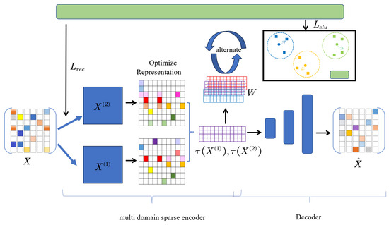
Figure 1. Sparse clustering algorithm flowchart under multi-domain autoencoder.

Each loss function part is as follows:

$$\begin{array}{ccc}{L}_{clu}\left(W\right)\hfill & =\hfill & L_{clu}^{\left(1\right)}\left(W^{\left(1\right)}\right)+L_{clu}^{\left(2\right)}\left(W^{\left(2\right)}\right)\hfill \\ \hfill & =\hfill & {\displaystyle \sum _{n=1}^N}{\displaystyle \sum _{u=1}^U}\left({\mathcal{L}}_u\left(X_n^{\left(1\right)};W^{\left(1\right)}\right){\parallel X_n^{\left(1\right)}-x_u^{\left(1\right)}\left(W^{\left(1\right)}\right)\parallel }_2^2\right.+\hfill \\ \hfill & \hfill & \left.{\mathcal{L}}_u\left(X_n^{\left(2\right)};W^{\left(2\right)}\right){\parallel X_n^{\left(2\right)}-x_u^{\left(2\right)}\left(W^{\left(2\right)}\right)\parallel }_2^2\right)\hfill \\ L_{rec}\left(W\right)\hfill & =\hfill & L_{rec}^{\left(1\right)}\left(W^{\left(1\right)}\right)+L_{rec}^{\left(2\right)}\left(W^{\left(2\right)}\right)\hfill \\ \hfill & =\hfill & {\displaystyle \sum _{n=1}^N}\left({\parallel X_n^{\left(1\right)}-{\widehat{X}}_n^{\left(1\right)}\left(W^{\left(1\right)}\right)\parallel }_2^2+{\parallel X_n^{\left(2\right)}-{\widehat{X}}_n^{\left(2\right)}\left(W^{\left(2\right)}\right)\parallel }_2^2\right)\hfill \\ L_{MD}\left(W\right)\hfill & =\hfill & \lambda L_{clu}\left(W\right)+L_{rec}\left(W\right)\hfill \end{array}$$

(4)

where $L_{clu}\left(W\right)$ is the clustering loss, $L_{rec}\left(W\right)$ is the reconstruction loss, and $L_{MD}\left(W\right)$ is the total loss under multi-domains. At this point, we have obtained the self-encoder in multi-domains.

3.2. Sparse L1 Regularization Model

We propose a sparse L1 regularization to generate sparsity in the model-training process. This integrated approach implements an adaptive penalty term on the weight matrix:

$$\begin{array}{c}\rho \left(W\right)=\sigma \left({\parallel W\odot \left(I-W\right)\parallel }_1+{\parallel W\parallel }_1\right)\hfill \end{array}$$

(5)

where $\sigma$ is the sparsity-induced function, taking the sigmoid function; ⊙ is the Hadamard product; ${\parallel ·\parallel }_1$ represents the L1 norm of weight matrix; and I is a all-one matrix with the same dimensions as W. The ${\parallel W\odot \left(I-W\right)\parallel }_1$ term penalizes the elements in the W matrix that are close to $0.5$, that is, W and $1-W$ will approach 0 at these positions. ${\parallel W\parallel }_1$ encourages the elements in W to approach 0, thereby achieving sparsity, and adjusts the degree of regularization accordingly based on the input parameters. Considering that we are studying a multi-domain problem where there are multi-network weight matrices, we rewrite $\rho \left(W\right)$ as ${\rho }_M\left(W\right)$

$$\begin{array}{c}{\rho }_M\left(W\right)={\displaystyle \sum _{m=1}^M}\sigma \left({\parallel W^{\left(m\right)}\odot \left(I-W^{\left(m\right)}\right)\parallel }_1+{\parallel W^{\left(m\right)}\parallel }_1\right)\hfill \end{array}$$

(6)

where m is the index of the domain, M is the number of domains (here $M=2$), and the weight matrices on the clustering layer are $W^{\left(1\right)}$ and $W^{\left(2\right)}$, $W=\left\{W^{\left(1\right)},\left.W^{\left(2\right)}\right\}\right.$. Apply it to the loss function and obtain the final loss function $L_{total}\left(W\right)$:

$$\begin{array}{c}{L}_{total}\left(W\right)=L_{clu}\left(W\right)+L_{rec}\left(W\right)+{\rho }_2\left(W\right)\hfill \end{array}$$

(7)

We employ the L1 norm to generate sparse solutions, optimizing the $0-1$ property of the function, and then utilize $\sigma$ to control the sparsity of function, thereby optimizing the calculation of clustering analysis errors. The flowchart is shown in Figure 2.

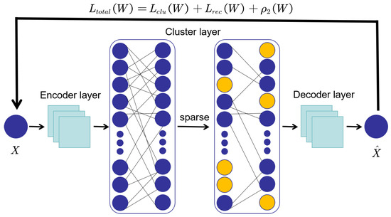
Figure 2. Algorithm flowchart for adding sparse L1 regularization terms.

As shown in Figure 2, we add the regularization term ${\rho }_2\left(W\right)$ to the loss function of the autoencoder in multi-domains. In the optimization process, some elements in the weight matrix of the clustering layer are penalized to become or approach 0. This also makes the proposed model robust to irrelevant or meaningless noise. This reduces the influence of noise features, making clustering more concentrated and accurate.

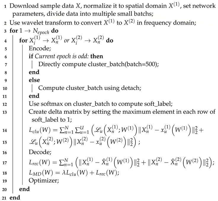
The algorithm is as shown in Algorithm 1. As for the complexity of the algorithm, the analysis is mainly divided into the following three parts. For the first part, the encoding and decoding process, the complexity is $O\left(P\right)$, and P is the dimension of the input sample data. For the second part, calculate the loss function, which includes calculating the time complexity of soft labels as $O\left(U\right)$, where U is the number of cluster centers; calculating the time complexity of hard labels as $O(batch\_size)$, where $batch\_size$ is the number of samples in each batch; and calculating the time complexity of delta as $O(batch\_size\times U)$. Thus, the reconstruction loss time complexity can be calculated as $O(batch\_size\times U)$ and the clustering loss time complexity as $O\left(P\right)$, so the time complexity of the loss function is $O(batch\_size\times U+P)$. For the third part, parameter updates and gradient updates have a time complexity of $O\left(P\right)$. The time complexity of updating cluster layer weights is $O\left(U\right)$, so the time complexity of parameter updates is $O(P+U)$. Consequently, the complexity of the proposed algorithm in each iteration is $O(3P+batch\_size\times U)$.

Algorithm 1: Sparse clustering algorithm based on multi-domain autoencoder.

Data: Random $80\%$ of training dataset X.

Result: Clustered loss $L_{clu}\left(W\right)$, reconstruction loss $L_{rec}\left(W\right)$, $NMI$, $ARI$, $ACC$, $AMI$, $Homogeneity$, $Complete$.

4. Experimental Results and Analysis

4.1. Experimental Setup and Datasets

In this experiment, we implement all the results on a 3-node, 90-core ThinkSystem SD630 306 V2 with Python 3.9 and PyTorch 2.0.1. The proposed method is evaluated using three datasets from the torchvision library: MNIST, CIFAR-10, and CIFAR-100 datasets. Specifically, the MNIST dataset consists of a widely used collection of handwritten digit images, including digits 0 to 9, with a total of 70,000 images divided into 10 classes. Each image is a 28 × 28 pixel grayscale image represented by a handwritten digit. The CIFAR-10 dataset is comprised of 60,000 RGB images, each measuring 32 × 32 pixels, and assigned to one of ten different classes. Similar to CIFAR-10, the CIFAR-100 dataset contains a set of 60,000 RGB images of size 32 × 32 × 3 from 100 fine-grained classes, which belong to 20 coarse-grained super-classes. The corresponding description is given in Table 1. It is worth noting that we conduct experiments on the 20 super-classes of CIFAR-100 and compare the performance on 20 super-classes.

Table 1. The used datasets.

Datasets	Classes	Size	Dimensionality
MNIST	10	70,000	28 × 28
CIFAR10	10	60,000	32 × 32
CIFAR100	100	60,000	32 × 32

The SMDR model utilizes a convolutional autoencoder to derive 10-dimensional features from the input data, which are subsequently employed for clustering purposes at the clustering layer. The encoder is made up of four convolutional layers conv(1,16,3,1,1)-conv(16,32,3,2,1)-conv(32,32,3,1,1)-conv(32,16,3,2,1), and then is followed by two fully connected layers fc(256)-fc(10). Here, conv(1,16,3,1,1) denotes the configuration of a convolutional layer with 1 input channel, 16 output channels, a convolution kernel size of 3, a stride of 1, and a padding of 1. Additionally, the notation fc(256) denotes a fully connected layer comprising 256 neurons. Batch normalization is implemented following each convolutional layer, with ReLU activation applied after each layer except for the final fully connected layer. The decoder component functions in an inverse manner to the encoder. The clustering layer is a fully connected layer that allows for the selection of the desired number of clusters. Both the convolutional autoencoder and the clustering layer are initialized randomly with Kaiming uniform [32], and then they are trained together for 3000 epochs using the default Adadelta [33] optimizer. In addition, there are no hyper-parameters that need to be tuned in our proposed method.

4.2. Experimental Results and Analysis

We adopt seven evaluation metrics to assess the experimental results, namely, Accuracy ($ACC$), Adjusted Rand Index ($ARI$), Normalized Mutual Information ($NMI$), Adjusted Mutual Information ($AMI$), Homogeneity ($Homo.$), Completeness ($Comp.$), and V-Measure ($V\_Mea.$). An important point to note is that higher values are preferable for all seven metrics. $ACC$ is the proportion of accurately predicted instances compared to the total number of instances. $ARI$ reflects the degree of overlap between two partitions. The Rand Index ($RI$) is defined as

$$RI=\frac{a+b}{\left(\frac{n}{2}\right)}\left(\frac{n}{2}\right)=C_n^2,$$

(8)

where a represents the number of instance pairs that are clustered in the same category C and in the same cluster K, and b is defined as the number of instance pairs that are categorized differently in C and clustered differently in K. Based on this, we define $ARI$ as

$$ARI=\frac{RI-E\left[RI\right]}{max\left(RI\right)-E\left[RI\right]}.$$

(9)

$NMI$ is used to measure the similarity of the clustering results. Mutual Information ($MI$) is defined as

$$MI\left(X;Y\right)=\sum _x\sum _{y}P\left(x,y\right)log\frac{P\left(x,y\right)}{P\left(x\right)P\left(y\right)},$$

(10)

where the joint distribution of two random variables $(X,Y)$ is denoted as $P(x,y)$, and their marginal distributions are represented as $P\left(x\right)$ and $p\left(y\right)$, respectively:

$$NMI\left(X;Y\right)=\frac{MI\left(X,Y\right)}{F\left(H\left(X\right),H\left(Y\right)\right)},$$

(11)

$H\left(x\right)$ represents the entropy of information, and $F(x,y)$ can be the min, max functions, geometric mean function, or arithmetic mean function. $AMI$ is denoted as

$$AMI\left(X,Y\right)=\frac{MI\left(X,Y\right)-E\left[MI\left(X,Y\right)\right]}{F\left(H\left(X\right),H\left(Y\right)\right)-E\left[MI\left(X,Y\right)\right]}.$$

(12)

$Homo.$ measures whether a clustering algorithm divides the data into homogeneous groups, meaning clusters consist solely of samples from the same category:

$$Homo.=1-\frac{H\left(C|K\right)}{H\left(C\right)}.$$

(13)

$Comp.$ is used to measure whether a clustering algorithm’s partitioning of data is complete, meaning whether samples from the same category are assigned to the same cluster:

$$Comp.=1-\frac{H\left(K|C\right)}{H\left(K\right)}.$$

(14)

$V\_Mea.$ is a comprehensive evaluation metric that takes into account both homogeneity and completeness, and it can be used to assess the quality of a clustering algorithm’s partitioning of data:

$$V\_Mea.=\frac{\left(1+\beta \right)\times Homo.\times Comp.}{\beta \times Homo.+Comp.}.$$

(15)

4.2.1. Experimental Comparisons

At the beginning of the experiment, we compare SMDR with seven popular clustering methods on the MNIST dataset. These methods include one deep learning-based clustering method (TELL [7]), two large-scale clustering methods (SLRR [34], LSC [35]), three subspace clustering methods (SC [36], LRR [37], LSR [38]), and vanilla k-means. It should be noted that we adjusted the hyperparameters of the methods being compared in the experiments. The results of the comparison are displayed in Table 2.

Table 2. Clustering performance on MNIST dataset.

Methods	NMI (%)	ARI (%)	ACC (%)	Parameter
SLRR	7.6	5.6	21.8	2.1
LSC-R	56.7	46.0	59.6	6
LSC-K	69.9	60.8	72.1	6
SC	73.2	62.2	71.3	1
LRR	10.4	10.0	21.1	10.01
LSR1	31.5	21.4	40.4	0.4
LSR2	30.0	20.0	41.4	0.1
k-means	77.8	70.5	78.3	—
TELL	82.8	75.9	80.8	—
SMDR	85.7	84.2	91.7	—

The clustering performance on the MNIST dataset displayed in Table 2, where bold numbers indicate data in which this model exceeds others, shows that SMDR outperforms the other clustering methods in all three evaluation metrics, demonstrating superior clustering performance on MNIST. Since TELL outperforms other clustering methods in the evaluation metrics, a more in-depth comparison with TELL will be conducted on the MNIST, CIFAR10, and CIFAR100 datasets to better understand the performance of SMDR.

4.2.2. The Comparison Results of SMDR and TELL on the MNIST Dataset

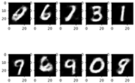
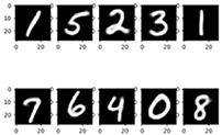
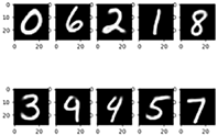
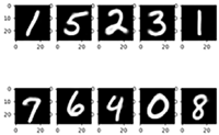
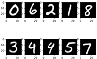
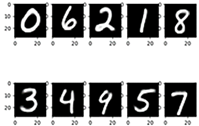
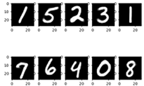
The comparison results of the clustering centers of SMDR and TELL on the MNIST dataset are shown in Table 3. During the training phase, both models are trained to identify the clustering centers of the MNIST dataset. Nevertheless, the TELL model exhibits an inability to accurately capture the entirety of these clustering centers. For instance, it is shown that at Epoch = 50, the model TELL encounters difficulty in accurately distinguishing between the digits “1”, “4”, and “9”, while the model SMDR demonstrates only a slight differentiation issue between the digits “4” and “9”. Although SMDR initially fails to separate “4” and “9”, it successfully distinguishes them when Epoch = 1000. During the training phase, both models are trained to identify the clustering centers of the MNIST dataset. Nevertheless, the TELL model demonstrates an inability to accurately capture the entirety of these clustering centers. For instance, it is shown that at Epoch = 50, the model TELL encounters difficulty in accurately distinguishing between the digits “1”, “4”, and “9”, while the model SMDR exhibits only a slight differentiation issue between the digits “4” and “9”. Notably, in this situation, TELL still has not managed to differentiate “1”, “4”, and “9”. Therefore, the proposed model achieves the global optimal faster compared to TELL.

Table 3. Comparison of clustering centers for SMDR and TELL [7] on the MNIST dataset.

	TELL [7]	SMDR
Epoch = 0
Epoch = 50
Epoch = 100
Epoch = 250
Epoch = 500
Epoch = 1000
Epoch = 3000

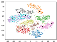
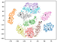
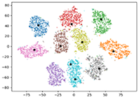
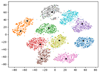
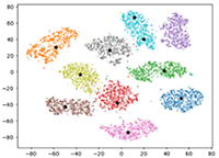
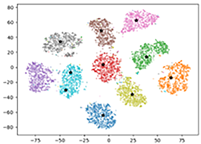
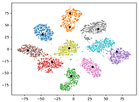
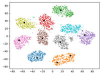
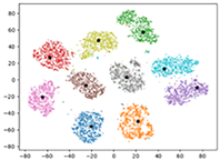
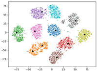
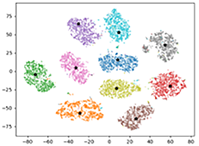
Table 4 presents a comparison of the clustering performance achieved by SMDR and TELL algorithms on the MNIST dataset. Both models successfully partition the dataset into ten clusters. However, it is shown that after multiple iterations, the SMDR clustering performance plot shows larger distances between clusters and tighter intra-cluster cohesion. In this situation, SMDR outperforms TELL in terms of clustering quality.

Table 4. Comparison of clustering performance for SMDR and TELL on the MNIST dataset.

	TELL	SMDR
Epoch = 0
Epoch = 50
Epoch = 100
Epoch = 250
Epoch = 500
Epoch = 1000
Epoch = 3000

The evaluation indicators of SMDR on MNIST are all higher than those of TELL as shown in the data in Table 5. Although the increase in some indicators is not obvious, the value of other indicators is greatly improved. As far as ARI is concerned, SMDR exceeds TELL by 8.3%, which means that the clustering results are more consistent with the labels, indicating that our proposed clustering algorithm has better performance. In particular, ACC is 10.9% higher than TELL, and the prediction accuracy is greatly improved, which can prove the superiority of the SMDR model.

Table 5. Clustering performance for SMDR and TELL on the MNIST dataset. Bold numbers indicate data in which this model outperforms other models.

				MNIST
	NMI (%)	ARI (%)	ACC (%)	AMI (%)	Homo. (%)	Comp. (%)	V_Mea. (%)
TELL	82.8	75.9	80.8	82.8	82.2	83.5	82.8
SMDR	85.7	84.2	91.7	85.7	85.7	85.8	85.7

4.2.3. The Comparison Results of SMDR and TELL on CIFAR Dataset

The clustering performance of SMDR and TELL on the CIFAR-10 dataset is presented in Table 6. It can be observed from Table 6 that the clustering evaluation metrics of SMDR and TELL on CIFAR-10 are not significantly different, with SMDR only surpassing TELL in terms of accuracy. For CIFAR-100, which has higher data complexity, we conduct clustering on its 20 super-classes, and the comparison of clustering accuracy is shown in Table 7. It is not difficult to see that SMDR has higher accuracy than TELL on super-classes such as S6 and S7. However, the difference in accuracy between the two methods is not significant in other super-classes. This demonstrates the excellent performance of SMDR on complex datasets.

Table 6. Clustering performance of SMDR and TELL on CIFAR-10 dataset. Bold numbers indicate data in which this model outperforms other models.

				CIFAR10
	NMI (%)	ARI (%)	ACC (%)	AMI (%)	Homo. (%)	Comp. (%)	V_Mea. (%)
TELL	10.5	5.3	23.1	10.5	10.2	10.8	10.5
SMDR	9.4	4.9	24.0	9.4	9.2	9.6	9.4

Table 7. Clustering accuracy on the 20 super-classes of the CIFAR-100 dataset. Bold numbers indicate data in which this model outperforms other models.

	S1 (%)	S2 (%)	S3 (%)	S4 (%)	S5 (%)	S6 (%)	S7 (%)	S8 (%)	S9 (%)	S10 (%)
TELL	36.2	37.9	31.9	33.0	38.8	30.9	30.4	32.1	30.6	32.0
SMDR	32.9	32.6	29.5	35.7	38.8	33.1	35.2	35.1	26.5	32.8
	S11 (%)	S12 (%)	S13 (%)	S14 (%)	S15 (%)	S16 (%)	S17 (%)	S18 (%)	S19 (%)	S20 (%)
TELL	43.8	27.9	28.1	31.2	25.8	35.6	32.3	33.1	30.1	41.0
SMDR	40.3	28.6	26.0	30.7	26.0	35.4	31.9	32.6	30.0	40.8

4.3. Ablation Study

To gain a more comprehensive understanding of the effectiveness and robustness of the method we proposed, we conduct three ablation studies based on MNIST. These studies involve evaluating the performance of SMDR with different model structures, loss functions, and optimizers.

4.3.1. Influence of Model Architecture

In previous experiments, SMDR relied on a convolutional autoencoder for feature extraction. To verify the robustness of our proposed method, we conduct comparative experiments between SMDR based on a fully connected autoencoder and vanilla k-means. The structure of the fully connected autoencoder is fc(500)-fc(500)-fc(2000)-fc(10), with ReLU activation used for each fully connected layer except the last one. The decoder is the reverse of the encoder.

Table 8 shows the comparison of clustering results of SMDR on MNIST based on different model structures. It is apparent that both the FCN-based SMDR and the CNN-based SMDR outperform their corresponding vanilla k-means in terms of evaluation metrics. Furthermore, due to the powerful feature extraction capability of the convolutional autoencoder, the CNN-based SMDR performs better in clustering than the FCN-based SMDR. This further highlights the advantage of SMDR in feature extraction.

Table 8. Influence of model architecture on the MNIST dataset. Bold numbers indicate data in which this model outperforms other models.

		FCN			CNN
	NMI (%)	ARI (%)	ACC (%)	NMI (%)	ARI (%)	ACC (%)
k-means	77.8	70.5	78.3	79.7	74.3	80.4
SMDR	82.9	82.2	91.5	85.7	84.2	91.7

4.3.2. Impact of Loss Function

In order to showcase the effectiveness of the sparse L1 regularization method that was previously proposed, we compare the performance of SMDR on the loss function with and without incorporating sparse L1 regularization. From Table 9, it is clear that the role of sparse L1 regularization in clustering is undeniable. This also proves that sparse L1 regularization can make some cluster weights in the clustering layer approach 0, thus making the clustering results more accurate.

Table 9. Impact of loss function on the MNIST dataset. Bold numbers indicate data in which this model outperforms other models.

	NMI (%)	ARI (%)	ACC (%)
Loss	82.8	75.9	80.8
Loss + sparse L1	85.7	84.2	91.7

4.3.3. Influence of Optimizer

In addition to the two ablation experiments mentioned above, we implement further evaluations of SMDR by employing different optimizers. In the experiment, we compare two popular optimizers (Adadelta [33], Adam [39]), both with default parameters. As shown in Table 10, it is indicated that SMDR using the Adadelta optimizer outperforms SMDR using the Adam optimizer.

Table 10. Influence of optimizer on the MNIST dataset. Bold numbers indicate data in which this model outperforms other models.

	NMI (%)	ARI (%)	ACC (%)
Adam	85.3	78.8	83.6
Adadelta	85.7	84.2	91.7

5. Conclusions

In this paper, we propose a sparse clustering model based on the multi-domain dimensionality reduction model to address the challenges in clustering high-dimensional data. The model synthetically learns the spatial and frequency domain invariant information in the data. Spatial information can provide useful information about the relationships between data points. Furthermore, we use discrete wavelet transform to project the spatial data into the frequency domain to provide local and frequency information. We integrate the sparse reconstruction process and sparse L1 regularization into the automatic encoder to complete the feature selection of high-dimensional data. After effective dimensionality reduction, the basic information of the original data is not lost, ensuring the accuracy of clustering. The sparse L1 regularization effectively increases the sparsity of the cluster layer weights, and improves the generalization performance and stability of the model. Finally, experimental results on MNIST, CIFAR10, and CIFAR100 database demonstrate the effectiveness of the proposed approach. In the future, we will focus on clustering on both high-dimensional and massive data.

References

- Yu, Y.; Liu, J. SCM enables improved single-cell clustering by scoring consensus matrices. Mathematics 2023, 11, 3785. [Google Scholar] [CrossRef]
- Sun, C.; Shao, Q.; Zhou, Z.; Zhang, J. An enhanced FCM clustering method based on multi-strategy tuna swarm optimization. Mathematics 2024, 12, 453. [Google Scholar] [CrossRef]
- Di Nuzzo, C. Advancing spectral clustering for categorical and mixed-type data: Insights and applications. Mathematics 2024, 12, 508. [Google Scholar] [CrossRef]
- Huang, D.; Wang, C.D.; Lai, J.H.; Kwoh, C.K. Toward multidiversified ensemble clustering of high-dimensional data: From subspaces to metrics and beyond. IEEE Trans. Cybern. 2022, 52, 12231–12244. [Google Scholar] [CrossRef] [PubMed]
- Jia, H.; Cheung, Y.M. Subspace clustering of categorical and numerical data with an unknown number of clusters. IEEE Trans. Neural Netw. Learn. Syst. 2018, 29, 3308–3325. [Google Scholar] [CrossRef] [PubMed]
- Hou, C.; Nie, F.; Yi, D.; Tao, D. Discriminative embedded clustering: A framework for grouping high-dimensional data. IEEE Trans. Neural Netw. Learn. Syst. 2015, 26, 1287–1299. [Google Scholar] [CrossRef] [PubMed]
- Peng, X.; Li, Y.; Tsang, I.W.; Zhu, H.; Lv, J.; Tianyi Zhou, J. XAI beyond classification: Interpretable neural clustering. J. Mach. Learn. Res. 2018, 23, 227–254. [Google Scholar] [CrossRef]
- Jing, L.; Ng, M.K.; Huang, J.Z. An entropy weighting k-means algorithm for subspace clustering of high-dimensional sparse data. IEEE Trans. Knowl. Data Eng. 2007, 19, 1026–1041. [Google Scholar] [CrossRef]
- Castelli, V.; Thomasian, A.; Chung-Sheng, L. CSVD: Clustering and singular value decomposition for approximate similarity search in high-dimensional spaces. IEEE Trans. Knowl. Data Eng. 2003, 15, 671–685. [Google Scholar] [CrossRef]
- Almalawi, A.M.; Fahad, A.; Tari, Z.; Cheema, M.A.; Khalil, I. k NNVWC: An efficient k -nearest neighbors approach based on various-widths clustering. IEEE Trans. Knowl. Data Eng. 2016, 28, 68–81. [Google Scholar] [CrossRef]
- Ordonez, C.; Omiecinski, E. Efficient disk-based k-means clustering for relational databases. IEEE Trans. Knowl. Data Eng. 2004, 16, 909–921. [Google Scholar] [CrossRef]
- Rathore, P.; Kumar, D.; Bezdek, J.C.; Rajasegarar, S.; Palaniswami, M. A rapid hybrid clustering algorithm for large volumes of high dimensional data. IEEE Trans. Knowl. Data Eng. 2019, 31, 641–654. [Google Scholar] [CrossRef]
- Guan, J.; Li, S.; Chen, X.; He, X.; Chen, J. DEMOS: Clustering by pruning a density-boosting cluster tree of density mounts. IEEE Trans. Knowl. Data Eng. 2023, 35, 10814–10830. [Google Scholar] [CrossRef]
- Zhao, X.; Nie, F.; Wang, R.; Li, X. Robust fuzzy k-means clustering with shrunk patterns learning. IEEE Trans. Knowl. Data Eng. 2023, 35, 3001–3013. [Google Scholar] [CrossRef]
- Yang, X.; Deng, C.; Dang, Z.; Tao, D. Deep multiview collaborative clustering. IEEE Trans. Neural Netw. Learn. Syst. 2023, 34, 516–526. [Google Scholar] [CrossRef]
- Xu, J.; Ren, Y.; Tang, H.; Yang, Z.; Pan, L.; Yang, Y.; Pu, X.; Yu, P.S.; He, L. Self-supervised discriminative feature learning for deep multi-view clustering. IEEE Trans. Knowl. Data Eng. 2023, 35, 7470–7482. [Google Scholar] [CrossRef]
- Zhao, Y.; Li, X. Spectral clustering with adaptive neighbors for deep learning. IEEE Trans. Neural Netw. Learn. Syst. 2023, 34, 2068–2078. [Google Scholar] [CrossRef]
- Guan, R.; Zhang, H.; Liang, Y.; Giunchiglia, F.; Huang, L.; Feng, X. Deep feature-based text clustering and its explanation. IEEE Trans. Knowl. Data Eng. 2022, 34, 3669–3680. [Google Scholar] [CrossRef]
- Li, S.; Liu, F.; Jiao, L.; Chen, P.; Li, L. Self-supervised self-organizing clustering network: A novel unsupervised representation learning method. IEEE Trans. Neural Netw. Learn. Syst. 2024, 35, 1857–1871. [Google Scholar] [CrossRef]
- Huang, Z.; Chen, J.; Zhang, J.; Shan, H. Learning representation for clustering via prototype scattering and positive sampling. IEEE Trans. Pattern Anal. Mach. Intell. 2023, 45, 7509–7524. [Google Scholar] [CrossRef]
- Wang, Z.; Ni, Y.; Jing, B.; Wang, D.; Zhang, H.; Xing, E. DNB: A joint learning framework for deep bayesian nonparametric clustering. IEEE Trans. Neural Netw. Learn. Syst. 2022, 33, 7610–7620. [Google Scholar] [CrossRef] [PubMed]
- Wang, T.; Zhang, X.; Lan, L.; Luo, Z. Local-to-global deep clustering on approximate uniform manifold. IEEE Trans. Knowl. Data Eng. 2023, 35, 5035–5046. [Google Scholar] [CrossRef]
- Chang, J.; Meng, G.; Wang, L.; Xiang, S.; Pan, C. Deep self-evolution clustering. IEEE Trans. Pattern Anal. Mach. Intell. 2020, 42, 809–823. [Google Scholar] [CrossRef] [PubMed]
- Ji, Q.; Sun, Y.; Gao, J.; Hu, Y.; Yin, B. A decoder-free variational deep embedding for unsupervised clustering. IEEE Trans. Neural Netw. Learn. Syst. 2022, 33, 5681–5693. [Google Scholar] [CrossRef] [PubMed]
- Li, X.; Zhang, R.; Wang, Q.; Zhang, H. Autoencoder constrained clustering with adaptive neighbors. IEEE Trans. Neural Netw. Learn. Syst. 2021, 32, 443–449. [Google Scholar] [CrossRef] [PubMed]
- Yang, L.; Fan, W.; Bouguila, N. Deep clustering analysis via dual variational autoencoder with spherical latent embeddings. IEEE Trans. Neural Netw. Learn. Syst. 2023, 34, 6303–6312. [Google Scholar] [CrossRef] [PubMed]
- Wu, L.; Yuan, L.; Zhao, G.; Lin, H.; Li, S.Z. Deep clustering and visualization for end-to-end high-dimensional data analysis. IEEE Trans. Neural Netw. Learn. Syst. 2023, 34, 8543–8554. [Google Scholar] [CrossRef] [PubMed]
- Wu, S.; Zheng, W.S. Semisupervised feature learning by deep entropy-sparsity subspace clustering. IEEE Trans. Neural Netw. Learn. Syst. 2022, 33, 774–788. [Google Scholar] [CrossRef]
- Wang, S.; Chen, Z.; Du, S.; Lin, Z. Learning deep sparse regularizers with applications to multi-view clustering and semi-supervised classification. IEEE Trans. Pattern Anal. Mach. Intell. 2022, 44, 5042–5055. [Google Scholar] [CrossRef]
- Cheng-Ru, L.; Ken-Hao, L.; Ming-Syan, C. Dual clustering: Integrating data clustering over optimization and constraint domains. IEEE Trans. Knowl. Data Eng. 2005, 17, 628–637. [Google Scholar] [CrossRef]
- Werner, D.H.; Allard, R.J. The simultaneous interpolation of antenna radiation patterns in both the spatial and frequency domains using model-based parameter estimation. IEEE Trans. Antennas Propag. 2000, 48, 383–392. [Google Scholar] [CrossRef]
- He, K.; Zhang, X.; Ren, S.; Sun, J. Delving deep into rectifiers: Surpassing human-level performance on imageNet classification. In Proceedings of the 2015 IEEE International Conference on Computer Vision (ICCV), Santiago, Chile, 7–13 December 2015; pp. 1026–1034. [Google Scholar] [CrossRef]
- Zeiler, M.D. Adadelta: An adaptive learning rate method. arXiv 2012. [Google Scholar] [CrossRef]
- Peng, X.; Tang, H.; Zhang, L.; Yi, Z.; Xiao, S. A unified framework for representation-based subspace clustering of out-of-sample and large-scale data. IEEE Trans. Neural Netw. Learn. Syst. 2016, 27, 2499–2512. [Google Scholar] [CrossRef] [PubMed]
- Cai, D.; Chen, X. Large scale spectral clustering via landmark-based sparse representation. IEEE Trans. Cybern. 2015, 45, 1669–1680. [Google Scholar] [CrossRef] [PubMed]
- Ng, A.; Jordan, M.; Weiss, Y. On spectral clustering: Analysis and an algorithm. Adv. Neural Inf. Process. Syst. 2001, 14, 849–856. [Google Scholar]
- Liu, G.; Lin, Z.; Yan, S.; Sun, J.; Yu, Y.; Ma, Y. Robust recovery of subspace structures by low-rank representation. IEEE Trans. Pattern Anal. Mach. Intell. 2013, 35, 171–184. [Google Scholar] [CrossRef]
- Lu, C.Y.; Min, H.; Zhao, Z.Q.; Zhu, L.; Huang, D.S.; Yan, S. Robust and efficient subspace segmentation via least squares regression. In Proceedings of the Computer Vision-ECCV 2012: 12th European Conference on Computer Vision, Florence, Italy, 7–13 October 2012; Part VII 12. pp. 347–360. [Google Scholar] [CrossRef]
- Kingma, D.; Ba, J. Adam: A method for stochastic optimization. arXiv 2014, arXiv:1412.6980. [Google Scholar] [CrossRef]
Disclaimer/Publisher’s Note: The statements, opinions and data contained in all publications are solely those of the individual author(s) and contributor(s) and not of MDPI and/or the editor(s). MDPI and/or the editor(s) disclaim responsibility for any injury to people or property resulting from any ideas, methods, instructions or products referred to in the content. |
© 2024 by the authors. Licensee MDPI, Basel, Switzerland. This article is an open access article distributed under the terms and conditions of the Creative Commons Attribution (CC BY) license (https://creativecommons.org/licenses/by/4.0/).