1. Introduction
Autonomous driving is an active research domain, pursued by both academia and private companies. Although fully automated driving, corresponding to the fifth level of automation [
1], has not been achieved yet, progress has been made on the various sub-problems underlying vehicle autonomous behavior, such as identifying and tracking objects, handling occlusions and varying light or weather conditions, predicting the trajectories and possible interactions of the agents in a traffic scene, route planning, and safety measures.
In this paper, we focus solely on the problem of trajectory prediction. This involves evaluating the possible future motion of traffic participants based on observed indicators in the recent past, such as positions, and sometimes heading angle, speed, or acceleration.
Trajectory prediction is a critical component of autonomous driving, allowing self-driving vehicles to anticipate the movement and behavior of other agents on the road, including other vehicles, pedestrians, bicycles, and more. It enables the vehicle to make informed decisions such as avoiding collisions, adjusting its speed and path, and anticipating traffic patterns.
To make accurate predictions, the vehicle must consider a wide range of inputs, including its own motion, the motion of other objects, road geometry, traffic signs, and environmental factors. By combining this information, the vehicle can build a predictive model of the environment, which it can use to make informed decisions about how to navigate the road safely and efficiently.
The main difficulties of the problem are related to the interactions of the agents, especially present in intersections, when a pedestrian approaches a crosswalk, or other situations where maneuvers are important, e.g., overtaking decisions, and also to the fact that trajectories may be multimodal, i.e., a common past set of observations may lead to different future trajectories.
Since the set of all possible maneuvers is virtually impossible to enumerate and evaluate exhaustively especially in situations with a large number of participants, the ego car needs to have an estimation about the most probable future states. Additionally, when the algorithms need to work in real time, i.e., on an actual autonomous car, computational efficiency becomes very important.
Accurate trajectory prediction is crucial for safe navigation. For example, safety can be increased if the ego car is able to predict whether another traffic participant will overtake another agent or if an agent in front will suddenly break. Furthermore, if autonomous vehicles are socially aware, their efficiency can be enhanced, and the overall traveling experience can become more comfortable.
The main contribution of this work is a neural network-based solution for predicting the future possible trajectories of traffic participants and their probabilities. By learning the effects of interactions between traffic participants, road features, and agent trajectories with different behavior patterns, the prediction quality can be improved.
This solution was developed as part of the PRORETA 5 project [
2], which aimed to build an autonomous vehicle that incorporates artificial intelligence methods. The trajectory prediction presented in this paper is only a component of the full autonomy stack of an actual self-driving car, which was demonstrated in Darmstadt, Germany, in October 2022.
The first component of the general architecture involved image processing based on visual saliency models. It focused on traffic participant detection and also used driver attention information. Object tracking was performed using radar and lidar data. The following component was the trajectory prediction module that will be described in the current paper. Based on the previous information, trajectory planning was performed using a trajectory tree that was iteratively created using Monte Carlo tree search. Finally, there was a safety check module based on classic logical rules rather than artificial intelligence methods. Another aspect of the project addressed the hardware configuration of the vehicle, including various sensors and cameras, as well as the human–machine interface.
The project addressed all the General Data Protection Regulation (GDPR) requirements of the European Union for the data captured by cameras. The original images used for training were only accessible to the image processing team and were stored in a secure environment. Subsequent work, including trajectory prediction, was performed on vectors of object data that no longer contained any user-sensitive information.
The rest of the paper is organized as follows. In
Section 2, we present an overview of the relevant literature.
Section 3 details our methodology and the structure of the training data. In
Section 4, we describe the developed model, while in
Section 5 we present the experimental results. Finally, in
Section 6 we include the conclusions and summarize the main findings.
2. Related Work
Many works address the problem of trajectory prediction. We would like to mention that the papers referenced for each category below are just examples and there are other authors that use those particular techniques as well.
Trajectory prediction methods can be broadly classified into two categories [
3]: model-based and data-driven methods. Model-based methods use mathematical models to represent the motion of agents on the road and to predict their future trajectories based on physical or kinematic principles. Several authors use, e.g., Kalman filters [
4], particle filters [
5], and non-linear models [
6]. On the other hand, data-driven methods rely on data to learn patterns and relationships in the motion of traffic participants and to make predictions based on these patterns. The most straightforward way of prediction is represented by rule-based methods, which use predefined rules to make predictions based on the behavior of road agents [
7]. Although a positive aspect is that they rely on explicit knowledge, in general, identifying the proper rules may take time and they may not generalize very well in various traffic conditions. Probabilistic methods model the uncertainty and variability in the motion of road agents and make predictions based on probability distributions, e.g., employing Partially Observable Markov Decision Processes (POMDPs) or Gaussian mixture models (GMMs), especially for maneuver-based trajectory prediction [
8,
9,
10].
The methods based on deep learning are arguably the most popular at this time and have contributed to a large extent to the state of the art. They use various kinds of deep neural networks to learn complex patterns from large amounts of training data and make predictions based on these patterns. A review of recent papers reporting such methods is [
11].
Recurrent Neural Networks (RNNs) are well-suited for sequential data and have been applied to trajectory prediction by encoding the past motion of agents into a hidden state and using this state to make predictions about their future motion. Long-Short Term Memory (LSTM) models, in particular, have been successfully used [
12,
13,
14,
15,
16]. The main advantage of recurrent networks is their ability to capture temporal dependencies, which is particularly relevant in the context of trajectory prediction, where the state of the traffic participants changes over time. Therefore, the models can incorporate complex patterns and trends in the data. Additionally, they can handle varying trajectory lengths. However, RNNs are complex models that usually require large amounts of data and may need long training times.
Convolutional Neural Networks (CNNs) are commonly used in trajectory prediction by utilizing image information from regular cameras, lidar sensors, or higher-level map projections [
17,
18,
19]. This type of neural network is well-suited to handle spatial information efficiently. Due to their use of parameter sharing, they typically have shorter training times for larger datasets and faster predictions. Still, CNNs have limitations when it comes to temporal information and context because they typically consider only a fixed window of input data at a time. In many cases, CNNs are used to process video inputs while LSTMs contribute to the encoding and decoding of trajectories.
Other papers have reported the use of Conditional Variational Autoencoders (CVAEs) [
20,
21,
22,
23]. CVAEs can generate diverse trajectories by sampling from the learned latent space, which can be advantageous in dealing with complex and diverse traffic scenarios where multiple plausible trajectories exist. They can also estimate uncertainty in the predictions by providing a probability distribution over the possible trajectories and can reconstruct missing or corrupted inputs that may occur when sensor data are affected by noise. Nevertheless, CVAEs are complex models that can be challenging to train and may not be suitable for real-time applications due to the computational expense of generating a diverse set of trajectories. Additionally, the quality of the learned latent space representation is critical to the model’s performance. If the latent space representation does not capture the underlying structure of the data, this can affect the output quality.
Generative Adversarial Networks (GANs) [
24,
25,
26] can also be used for trajectory prediction. They can also generate diverse trajectories by training the model to create realistic trajectories that are expectantly indistinguishable from real ones. Many of the advantages and disadvantages of CVAEs apply to GANs as well. However, an additional issue related to both architectures is mode collapse, when the model generates only a small subset of possible trajectories while ignoring the rest, and this can lead to similar and unrealistic results.
Attention mechanisms [
12,
27] can also be used in conjunction with various models for trajectory prediction. They can capture global context by allowing the model to attend to different parts of the input sequence when generating the output sequence. This can be advantageous when dealing with complex and diverse traffic situations, where the context of the entire scene can be important for prediction. In many works, attention mechanisms refer to social attention, which can selectively aggregate information from nearby agents to predict the trajectory of the target agent. In this way, they capture the dependencies between the target agent and the scene context. This model has shown improved performance over other social pooling methods. Conversely, attention mechanisms can increase the complexity of the model and make it more difficult to train. They can also suffer from attention drift, where the model attends to irrelevant parts of the input sequence as the output sequence progresses, resulting in the model generating unrealistic trajectories.
Graph Neural Networks (GNNs) are suitable for modeling complex interactions between traffic participants by encoding the relationships between nodes (representing agents) and edges (representing interactions) in a graph structure [
28,
29,
30,
31]. GNNs can incorporate spatial information by using the relative positions of the nodes in the graph, which can be useful for trajectory prediction in complex scenarios. They can also scale to large graphs, which is important for modeling intricate traffic scenes. Yet GNNs require a large amount of data and are computationally expensive to train, especially for large graphs with many nodes and edges.
Transformer networks [
32,
33,
34] represent a relatively recent architecture where operations can be highly parallelized, leading to faster training and inference times compared to sequential models such as LSTMs. Like the latter, they can capture both long-term dependencies and global context by attending to all positions in the input sequence. A disadvantage is that transformer networks may require large amounts of data to learn effective representations of the input sequence and may struggle to generalize to new and unseen scenarios, as they can be sensitive to the specific structure of the input sequence.
It must be emphasized that most approaches actually use hybrid methods, which combine the strengths of multiple techniques to make predictions.
Another direction related to reinforcement learning (RL)—in fact, inverse RL—is to use imitation learning to find out driving policies by estimating the cost function of human drivers [
35].
Depending on the abstraction of level on which prediction is made, there are physics-based, maneuver-based, and interaction-aware motion models [
36]. Physics-based models apply the laws of physics to estimate the trajectory, based, e.g., on speed, acceleration, steering, etc. They are useful as classic fail-safe techniques, but in general they are reliable only for short-term predictions. Maneuver-based models try to identify the maneuvers of the road agents but usually in isolation, while interaction-aware models take into account the influence of the neighbors on an agent but are more computationally complex.
Multiagent systems have also been used in the context of trajectory prediction to model the behavior of multiple agents in a scene, such as pedestrians or vehicles, and predict their future movements based on their past behavior and interactions with other agents. They are especially valuable for the latter, because interactions between agents play a crucial role in determining their future movements. Various methods have been proposed to model them, such as social force [
37] or game theoretic [
38] models.
Even if research on trajectory prediction constantly evolves, there are several key issues that still pose some challenges to the public use of autonomous vehicles. First, one can mention interpretability, i.e., the development of methods for making the predictions of autonomous vehicles explicit, so that the reasoning behind their decisions can be understood by humans. Secondly, one can think of interaction and cooperation between autonomous vehicles, i.e., how they can communicate and cooperate with one another to improve safety and efficiency on the road. Thirdly, there is the problem of unstructured and dynamic environments, which creates the need to develop prediction models that can handle complex, dynamically changing scenarios, such as urban environments with heavy traffic.
3. The Structure of the Training Data
The trajectory prediction problem can be formalized as follows. Let be an observation vector with the position and possibly other motion indicators for agent i at time step t. If p designates the present time step, then for agent i the past trajectory (the input of the machine learning model) is a sequence of nin vectors {,…, , }. The output of the model is the predicted trajectory, which is another sequence of nout vectors {, ,…, }. In our case, the output consists of a set of such future trajectories, each with its corresponding probability.
The data that serves as an input to the model results after the segmentation and identification of the objects in the scene. The inputs refer to the representation of traffic participants (agents) and the representation of the road. In this approach, we considered the past information about an agent, the group context information, i.e., the surrounding agents, and the road context. An overview of the method is presented in
Figure 1. The training phase uses information about the current agent’s past trajectory and its desired trajectory, the group context that includes information about the past states of the surrounding agents, and road context that includes information about the road structure. The inference phase uses information about the past trajectory of the current agent, the group context, and the road context.
3.1. The Input Vectors
3.1.1. Agent Trajectory Representation
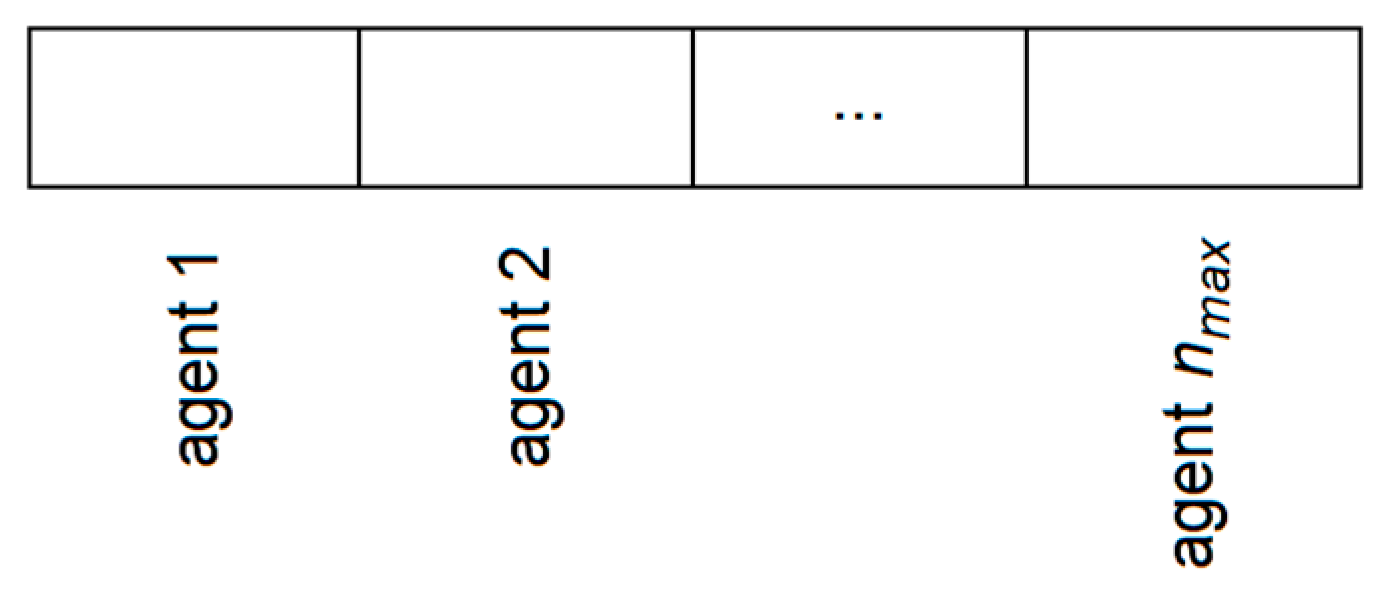
The presented approach aims to handle a variable number of agents of different types. Since the inputs to the neural model have a fixed size, we use a maximum number of agents
nmax (
Figure 2). When an observation is processed, the identified objects are considered “real” agents, and the rest, the unused placeholders, are considered “dummy” agents. The information corresponding to the dummy agents is ignored in the processing using a mechanism described in
Section 4.1. In our case studies,
nmax = 10.
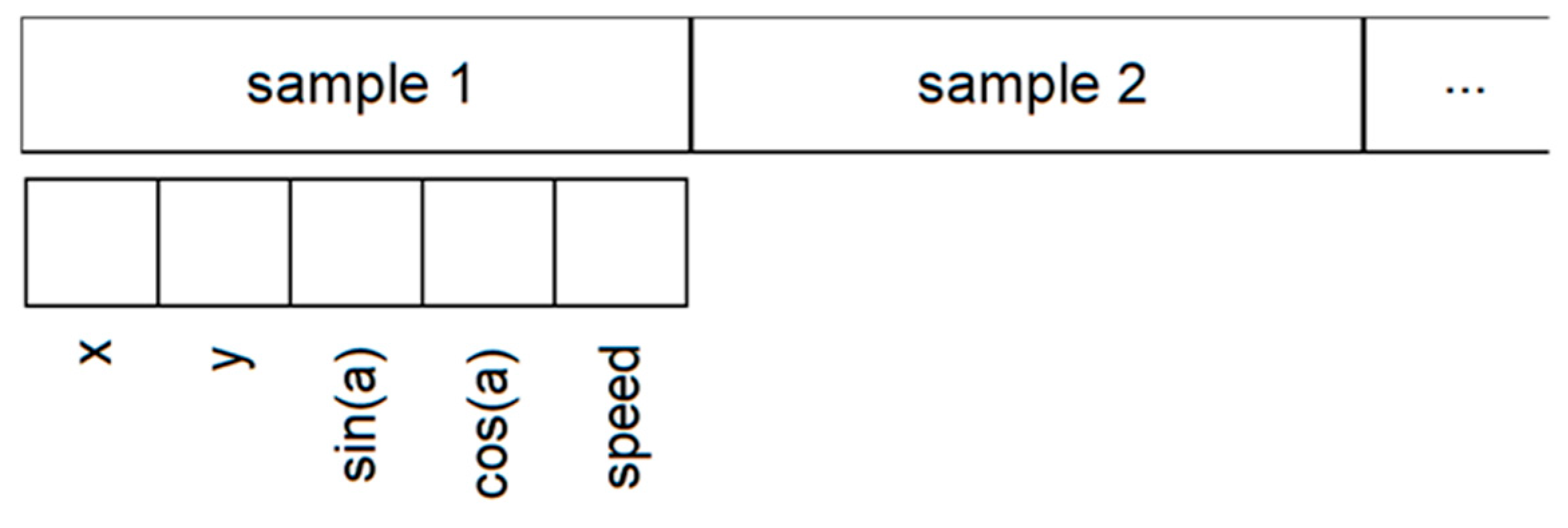
The first components of an input block corresponding to an agent are displayed in
Figure 3.
The rest of the input vector contains information about the past trajectory of the agent, including the present state. The trajectory is discretized into
nin samples (in our case,
nin = 10), as shown in
Figure 4.
For our problem, the x coordinate is normalized between –10 m and 10 m relative to the center line of the road. The y coordinate is normalized between –150 m and 150 m. Thus, the positions of the agents are in fact Frenet coordinates (described in the next paragraph) relative to the present position of the ego vehicle: x corresponds to the lateral displacement (the Frenet coordinate d) relative to the center line of the road, and y corresponds to the longitudinal displacement (the Frenet coordinate s) but relative to the ego agent position. The use of Frenet coordinates has the advantage that it avoids special cases caused by the change of perspective in curves and which may need more training data to cover various types of curves. Using the presented approach, curves are handled in the same way as straight road segments.
If the coordinates of the points representing the curve are in a Cartesian coordinate system, the Frenet transformation (
Figure 5) interpolates linearly between the supporting points of the base curve. For the transformation of a 2D pose from Cartesian to Frenet coordinates, it is necessary at first to find the closest linear segment to the Cartesian coordinate. To find the point where the object is projected on this line, the perpendicular vector of the reference path is generated and it is intersected from the object position with the reference path. This results in the distance of the object to the reference path and the distance from the beginning of the path. The Cartesian points can fall onto areas where no perpendicular line can be drawn to a linear spline segment of the base curve, or where a perpendicular line can be drawn to two adjacent linear spline segments; a curve at that point is either convex or concave. In that case, the point is always projected on the first of the two segments. To transform a 2D pose from Frenet to Cartesian coordinates, a linear interpolation is used between the supporting points of the base curve even with the heading angle. A continuous distance function is employed, so that every point in the coordinate system is well defined.
For the heading angle, simply normalizing a value between [0, 2π) or [0°, 360°) introduces a discontinuity when the angle is around 0. This may happen very often since the “moving straight ahead” angle is considered 0. Therefore, a tuple (sin(a), cos(a)) is used to represent the angle. In this way, the variations are continuous for any value of the angle.
Finally, a trajectory sample contains the instantaneous speed measured in m/s.
An improvement of the representation of the y coordinate takes into account the fact that drivers usually pay more attention to the traffic participants nearby than to those situated at longer distances, especially in urban scenarios with lower speeds than highways and with more agents at lower distances.
Therefore, a technique that we name “focused normalization” can be used, which warps the longitudinal coordinate space in order to provide more details about the short-distance agents and fewer details about the long-distance ones (
Figure 6).
This transformation uses a sigmoid function to change the
y coordinate:
where
λ is a coefficient that controls the width of the non-saturated region of the sigmoid function. In our case studies,
λ = 2.5.
3.1.2. Group Context Representation
The group context is considered in a similar way as the agent trajectory representation. For each agent, the surrounding agents that can influence the behavior in traffic are considered, and we are including the ones that are around the current agent, e.g., 50 m around. As mentioned before, because the number of agents in the nearby area is variable and the inputs to the neural model have a fixed size, we use a maximum number of context agents nn. For each agent included in the context, we have the agent type: (flags [0/1] [real/dummy agent] [is car] [is obstacle] [is bicycle] [is pedestrian] [is truck/bus]). For example, a truck can be defined as 100,001 and a bicycle as 100,100. For each past point, we consider the coordinates x, y, the pair sin(a), cos(a), where a is the heading angle, and the speed.
3.1.3. Road Context Representation
The road representation takes into account information about a general area (e.g., 40 m) around the ego agent (longitudinally) and complete information on the width of the road (transversally). Each traffic participant is considered ego in turn for trajectory prediction; therefore, road information may be slightly different for each traffic participant. Each road segment is encoded taking into account the following:
The segment type: driving lane (100), parking (010), sidewalk (001). One-hot encoding is used, and more types can be included (e.g., crosswalks);
The distinction between a real road segment or a dummy one (in the form of a binary flag), to account for a variable number of segments.
For each lane in the sight of view, five waypoints are encoded on the center of the lane, at −20 m, −10 m, 0 m, 10 m and 20 m relative to the y coordinate of the ego vehicle. Each waypoint is identified by (x, y, sin(a), cos(a)), where a is the angle of the road segment (e.g., 0 for “up”/the same direction as the ego, π or 180° for “down”/opposite direction). For a straight road, only 0° and 180° values are possible, therefore (sin(a), cos(a)) may be replaced by a binary 0/1 flag or a 01/10 encoding. For intersections, actual angle values are useful.
Each road segment, roughly defined by a quadrilateral, is also encoded by means of the four defining points (xi, yi) also relative to the ego agent. Their y coordinates are always clipped to the (−20 m, 20 m) range.
In addition, eight values are included for the corners of the rectangle. All in all, there are 32 values for a lane.
For the situation displayed in
Figure 7, the following road information would be used:
S1 (parking lane): [1] [0 1 0] [−5 −20 0 0] … [−5 20 0 0] [−6 −20] … [−6 20];
S2 (driving lane): [1] [1 0 0] [−2 −20 0 −1] … [−2 20 0 −1] [−4 −20] … [−4 20];
S3 (driving lane): [1] [1 0 0] [2 −20 0 1] … [2 20 0 1] [0 −20] … [0 20];
S4 (parking lane): [1] [0 1 0] [5 −20 0 0] … [5 20 0 0] [4 −20] … [4 20].
In the model, each road segment is encoded into an embedding, as shown in
Section 4.1. All the real (non-dummy) segment embeddings are encoded into segment embeddings using max pooling. The resulting road segment features are concatenated with the embeddings of the traffic participants, as part of the context.
3.2. The Output Vectors
Most of the information is contained in the input vectors. Comparatively, the structure of the output vectors is much simpler. It provides predictions for nout steps into the future (in our case, nout = 20). The predictions are made only for the ego agent; therefore, an output vector is a list of nout tuples of (x, y, sin(a), cos(a), speed).
The ego car needs estimates about the future trajectories of all active traffic participants. Thus, for prediction, each non-dummy agent becomes the ego agent in turn and the model presented in
Section 4.1 predicts its possible future trajectories. All these predicted trajectories are further used by the actual ego vehicle for trajectory planning.
4. The Proposed Model
As a distinct feature of the present approach, we use vectors of agent features as inputs into our model, rather than images, because we assume that a segmentation of the image has been performed in a previous step. This was conducted by a different team in the PRORETA 5 project mentioned in the Introduction. However, a large part of the existing work on trajectory prediction takes images as input. Although this may seem like an insignificant difference, working with vectors instead of images proved to have a big influence on the performance of the learning models, because several models proposed as recent state of the art performed worse than expected on this modified problem. Additionally, generative models such as CVAE need some time for sampling to assess the probabilities of different modes, and this may hinder their use for real-time applications. These are the reasons that lead us to develop the model described in this section.
4.1. Network Architecture
In order to correctly predict the movement of the surrounding agents, the system needs to account for their multimodal nature. Thus, we capture the idea that the same history may lead to multiple possible futures. For example, a car closing in behind the ego vehicle may follow it in the next predictable future or may overtake it. Both futures are possible, but the past trajectory of the approaching vehicle is the same in both cases. Based on such previous situations found in the training set, the model needs to compute multiple future trajectories (i.e., modes) and their probabilities.
The proposed model is therefore a neural network with
n output heads, one for each mode. Its architecture is presented in
Figure 8.
There is an encoding part for the ego vehicle and also for the rest of the agents (the closest nn agents to the ego agent; in our case, nn = 9). That consists in three fully connected layers with a leaky ReLU (leaky rectified linear unit) activation function for each case to encode the input information.
For the rest of the agents, a symmetric function must be used to represent the context, because such a function is insensitive to the order in which its operands are considered. In our case, a max pooling component is applied to the embeddings of the other traffic participants. When an agent is a dummy, its embedding is ignored: the embedding is multiplied by the 1/0 flag that shows whether the agent is real or a dummy; therefore, the embedding of a dummy agent becomes a vector of zeros. The context embedding is responsible for capturing the interactions between agents in an implicit form.
The road information is embedded using a similar approach like in the group context. That consists in three fully connected layers with a leaky ReLU activation function for each case to encode the input information, followed by the max pooling component.
The decoding part of the network extracts the information for future trajectories using three fully connected layers with a leaky ReLU activation function and a second fully connected layer with a sigmoid (logistic) activation function.
The outputs represent the future trajectories with a probability for each mode: m trajectories each with my steps into the future plus one value denoting its probability. In our case, m = 3 for the multimodal and of course m = 1 for the unimodal case.
4.2. The Conditional Loss Function
The training of the model is based on a conditional loss function (inspired by [
39]) made up of two terms:
where
pi is the probability of mode
i and
ei is the MSE between the desired trajectory vector and the trajectory vector predicted by mode
i. By minimizing
L1, when
pi is high (the mode matches the current instance well),
ei will further decrease, but when
pi is low, the influence on
ei will be small. Therefore, the effect of
L1 is especially strong for the modes with high probabilities. This is in fact a mixture-of-experts loss, where the computed value is an expected MSE given the probabilities of individual “experts”, in our case, the individual modes.
On the one hand, L2 tries to decrease the MSE, that is, to bring the predicted trajectory closer to the desired trajectory for that mode. On the other hand, it tries to increase the probability of the best mode. If the probability of one mode increases, the probabilities of the other modes automatically decrease. This second term of the L2 loss function is actually a form of cross-entropy loss. Ideally, the best mode should match the current instance perfectly, and, therefore, its target value for the probability is 1, so the second term in Equation (3) is actually . The other modes should not predict the instance, and so their target values for the probability are 0, which cancel the terms . The term ei imposes that the best mode becomes even closer to the desired trajectory of the current instance.
One implementation note may be useful. Since the neural network model was developed with PyTorch [
40], the conditional loss involving the finding of the best mode is not straightforward, because a function involving “if” branches may not be continuous and thus not differentiable. Therefore, a matrix
A is computed for each mode such that
Aji = 1 if mode
i is the best mode for instance
j and 0 otherwise. The implemented expression for
L2 is actually
The loss function is computed for one instance at the time; that is why j does not appear explicitly in Equation (4), but the losses corresponding to all instances in a training batch are eventually summed together.
The final composite loss is the sum of these two functions:
It causes the modes to specialize on distinct classes of agent behaviors, e.g., going straight or turning. Implicitly, this composite loss function encourages a clustering behavior of the modes over the predicted trajectories.
Computing the Mode Probabilities
The values computed by the neural networks for each mode must be converted into a valid probability distribution. This may seem simple at first sight, but it needs special attention because the training process is very sensitive to small probabilities given their use in the loss function, especially when it handles the situations when probabilities are very small, in fact close to 0, and this is often the case for unimodal trajectories. It was empirically found that different transformation formulas for avoiding the cases of 0/0 or log(0) lead to quite different results.
For example, a simple way of avoiding a zero division is to use a small non-zero number
ε in the denominator when normalizing the probabilities:
However, when the values provided by the neural networks are all very small, this equation may lead to invalid results. Let us assume a situation with two modes, with the computed values (0, 0). The probabilities according to Equation (6) are (0, 0). If the computed values are (0, ε), the probabilities according to Equation (6) are (0, 0.5). Since their sum is not 1, this is not a valid probability distribution.
The variant finally chosen for probability normalization is presented below:
First, the values from the neural network are scaled such that 0 becomes ε and 1 becomes 1 − ε. The middle value of 0.5 remains unchanged. This is possible because the sigmoid activation function of the neural network provides values only in the [0, 1] interval. Secondly, the values are normalized to create a valid probability distribution, but without the risk of having a division by zero. In this case, (0, 0) becomes (0.5, 0.5) and (0, ε) becomes (0.33, 0.67). Larger values provide normally expected results, e.g., (0.4, 0.7) becomes (0.36, 0.64).
4.3. The Fine-Tuning Loss Function
Since the training instances may be affected by noise and variability, a dilemma appears between fitting the training data as well as possible vs. ensuring a good generalization for new situations, especially because the model is meant to be used in a real-world urban scenario on an actual car. A similar problem is present, e.g., when assessing the value of the C parameter for support vector machine (SVM) models, where it controls the balance between trying to create a precise model and allowing training errors to increase the generalization capability.
In our case, if the trajectory points are not identical, overfitting causes mode collapse, where all instances are assigned to a single mode. However, a model with incomplete training may not be affected by this, and thus similar past histories may be assigned multiple modes, but also the training error is larger than desired.
Therefore, we decided to train the model for fewer training epochs, and finally added a fine-tuning phase to decrease the error of the predicted trajectories without changing their probabilities.
For this purpose, a mask
M is calculated that identifies the dominant mode for each training instance. The outputs corresponding to the predicted trajectory points only for the mode with the lowest MSE are assigned a value of 1, and the rest remain 0. The outputs related to the probabilities also have their mask values equal to 0. Thus, the fine-tuning loss is defined as the mean square loss only for the elements identified by the mask:
where
k is the index of the elements of vectors
y (the predicted network output),
yd (the desired output), and the columns of
M (the mask), while
j denotes a training instance. Basically,
Lft computes the MSE only for the elements included in the mask.
Although only two training cycles were adopted in the present case studies. i.e., one conditional training phase and then one fine tuning phase, it is possible to have more such alternating phases iteratively, in order to enhance both the multi-modal trajectory probabilities and the quality of the trajectories.
5. Case Studies
5.1. Simple Bimodal Trajectories
In this section, we include two very simple problems to demonstrate more clearly the type of problems addressed in our work and the obtained results. These trajectories have only two modes, and the network architecture is simpler, with a (3:24:3) configuration, i.e., 3 inputs, 24 neurons in a hidden layer, and 3 outputs.
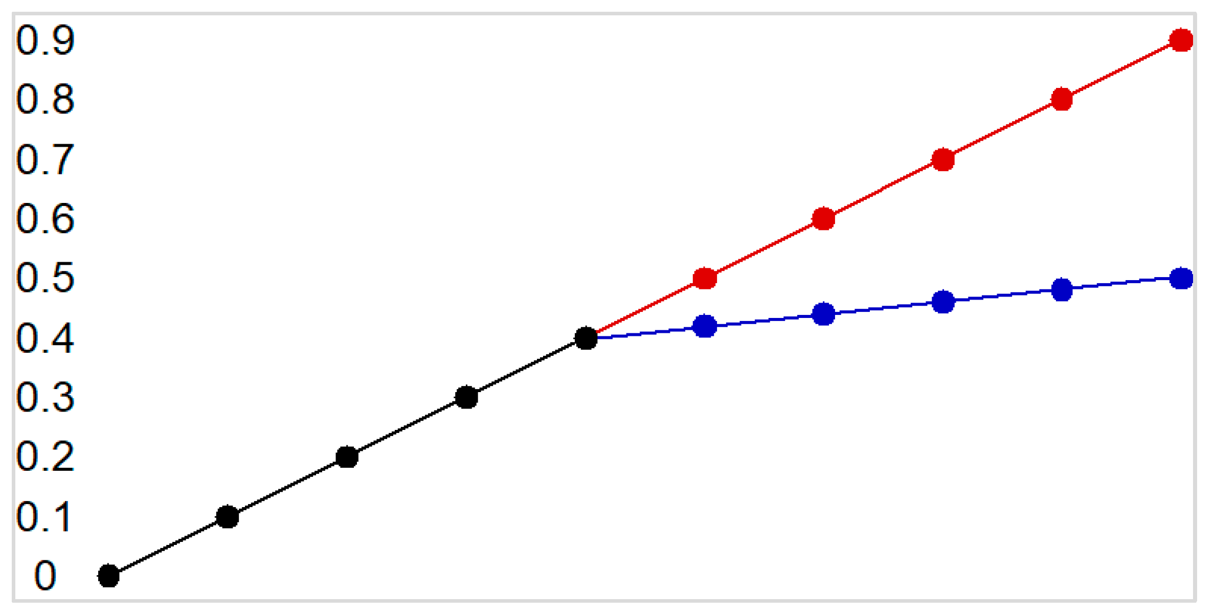
First, let us consider a dataset of 1D trajectories with three points in the past and present and three points to be predicted in the future, as displayed in
Table 1. These instances correspond to the multimodal trajectory problem displayed in
Figure 9. One can see that the first five points are common between the two possible trajectories that diverge afterwards. Since only three points are considered in an instance, the model should identify the two possible trajectories for the inputs in instances 1–3, which are the same as in instances 6–8. Then, the inputs in instances 4–5 and 9–10 should uniquely identify a specific trajectory.
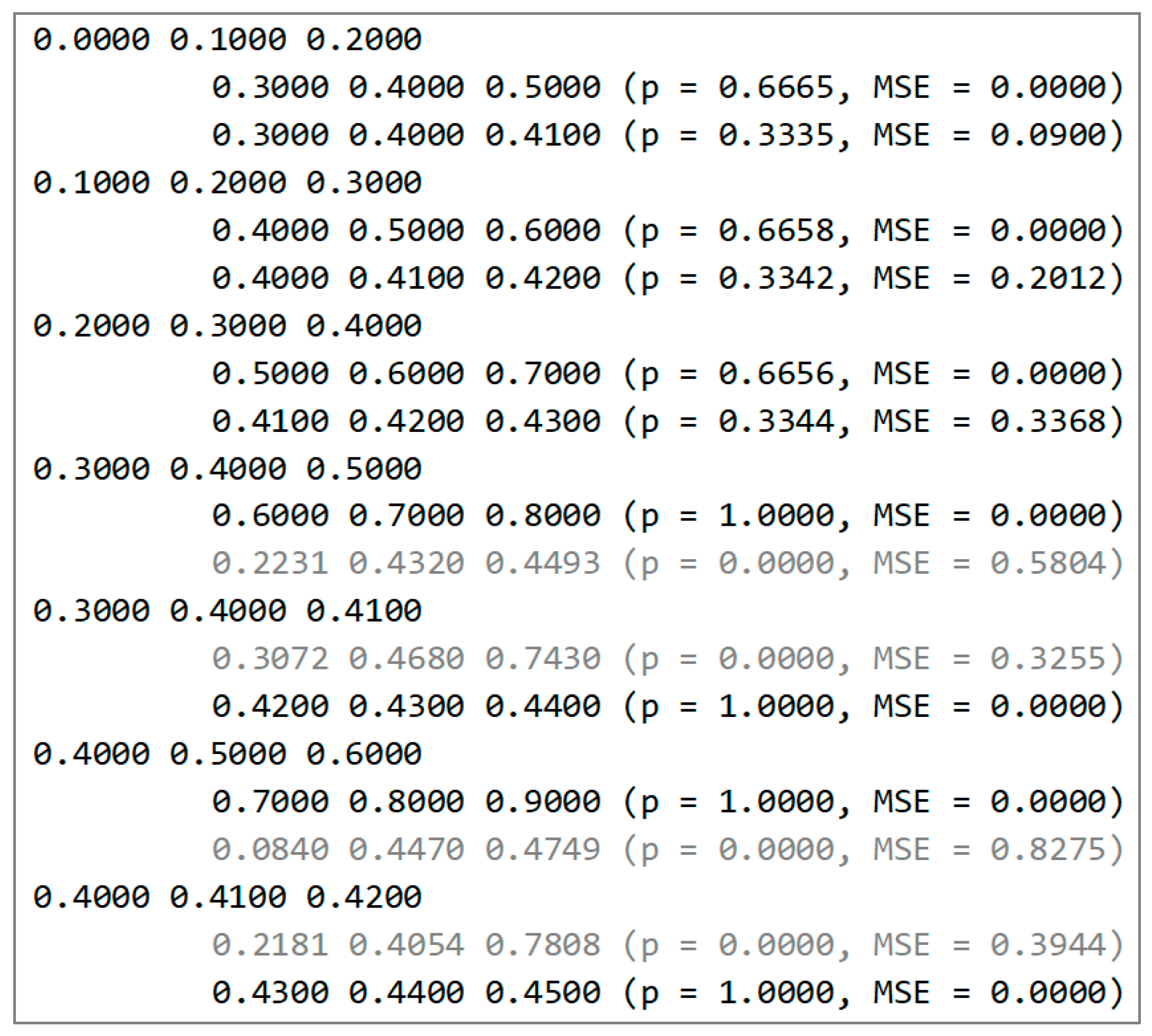
The obtained results are presented in
Figure 10. The instances with the same inputs are not repeated, because the results would be the same. These results can be interpreted as follows. The unindented lines represent the three inputs’ points. Then, the next two lines represent the computed outputs. In each such line, the three output values are presented. In the brackets,
p (the probability of a mode) and the MSE between the model output and the actual output are included. The content of lines 1–3 corresponds to instance 1 in
Table 1; that is why the MSE in line 2 is much smaller than that in line 3, because the MSE is computed for the desired output of instance 1. If we had repeated the inputs for instances 6–8, the MSE corresponding to the second mode would have been close to 0.
Because the dataset is balanced between the two modes, the probabilities for the first three cases are close to 0.5. The last four cases are the situations where the future trajectory can be uniquely determined from the inputs, thus the result is unimodal. The probability of the dominant mode is close to 1, and the other mode, with a probability close to 0, is represented in gray. Still, it is interesting to see that the inactive modes continue the trends of their learned trajectories, either with a larger slope (the red one) or with a smaller slope (the blue one).
The dataset in
Table 2 shows a similar situation, but the first five instances are repeated at the end in order to give them a higher weight in the computation of probabilities, because the network will encounter that case more frequently.
The results included in
Figure 11 show that the probability of the corresponding mode increases to 0.67 as expected, while the unimodal trajectories are still identified by probabilities close to 1.
Again, the non-selected modes still capture an approximation of the other “would-be” trajectory, e.g., going to 0.78 in the last case (according to the red trend), or to 0.47 in the penultimate one (according to the blue trend).
5.2. The inD Dataset
Our main case of study is based on the inD dataset (Intersection Drone Dataset) [
41], a recently compiled collection of vehicle trajectories recorded at intersections in Germany using a drone. This method of data collection eliminates the limitations commonly encountered with conventional traffic data collection techniques, such as occlusions. Utilizing modern computer vision algorithms, the positional error is typically within 10 cm. Traffic was recorded at four different intersections and the trajectories of each road agent and its respective type have been extracted. The types of the traffic participants available are cars, buses or trucks, bicyclists, and pedestrians.
5.2.1. Implementation Details
For the InD dataset, for intersection A, information about each class of agent was extracted separately because a distinct model was trained for each type. The dataset contains 135,956 instances, of which 74,530 correspond to cars, 4518 correspond to buses or trucks, 51,121 correspond to pedestrians, and 5787 correspond to bicyclists. Of these instances, 25% were used for testing. Overall, 101,967 instances were used for training, and 33,989 instances were used for testing. The results presented in
Section 5.2.2 were obtained only for the testing set.
The predicted trajectories correspond to a 5 s time horizon with 20 trajectory points, each at 0.25 s intervals. To train a model, 100,000 epochs are used, which are split into two parts: the conditional training phase and the fine-tuning phase, as described in
Section 4.2 and
Section 4.3. For each model, the process takes approximately 4 h on a HP Z4 G4 station with a 3.6 GHz Intel 4 Core Xeon W-2123 processor, 32 GB of RAM, and an nVidia GeForce RTX 2080 graphics card.
During the experiments, different optimizers were used, including RMSProp (Root Mean Squared Propagation) and SGD (Stochastic Gradient Descent), as well as different types of activation functions for the hidden layers, such as sigmoid, hyperbolic tangent, ReLU (Rectified Linear Unit), and ELU (Exponential Linear Unit), together with different learning rates. Empirically, it was found that the configuration displayed in
Figure 8 and the Adam optimization algorithm with a learning rate of 10
−3 provided the best results.
5.2.2. Evaluation Metrics
The average displacement error (ADE) and the final displacement error (FDE) are the two most commonly applied metrics to measure the performance of trajectory prediction.
ADE is the average Euclidian distance between the desired data and the predicted data, summed over all time steps:
where
T is the number of prediction steps,
x and
y are the predicted coordinates and
xd and
yd are the desired values, i.e., the ground truth.
FDE measures the Euclidian distance between the desired final position and the predicted final position:
It measures the ability of a model to predict the destination and is more challenging as errors accumulate over time.
In our experiments, we evaluate the unimodal approach prediction and the best prediction for multimodal approach. We consider the best prediction the one that has the smallest ADE and FDE among the three predicted trajectories.
For each type of traffic participant such as car, truck, bicyclist, or pedestrian, a different model is trained in order to learn the specific behavior that depends on the class of the agent. In
Table 3 and
Table 4, the results for each type of agent in unimodal and multimodal settings are presented.
In
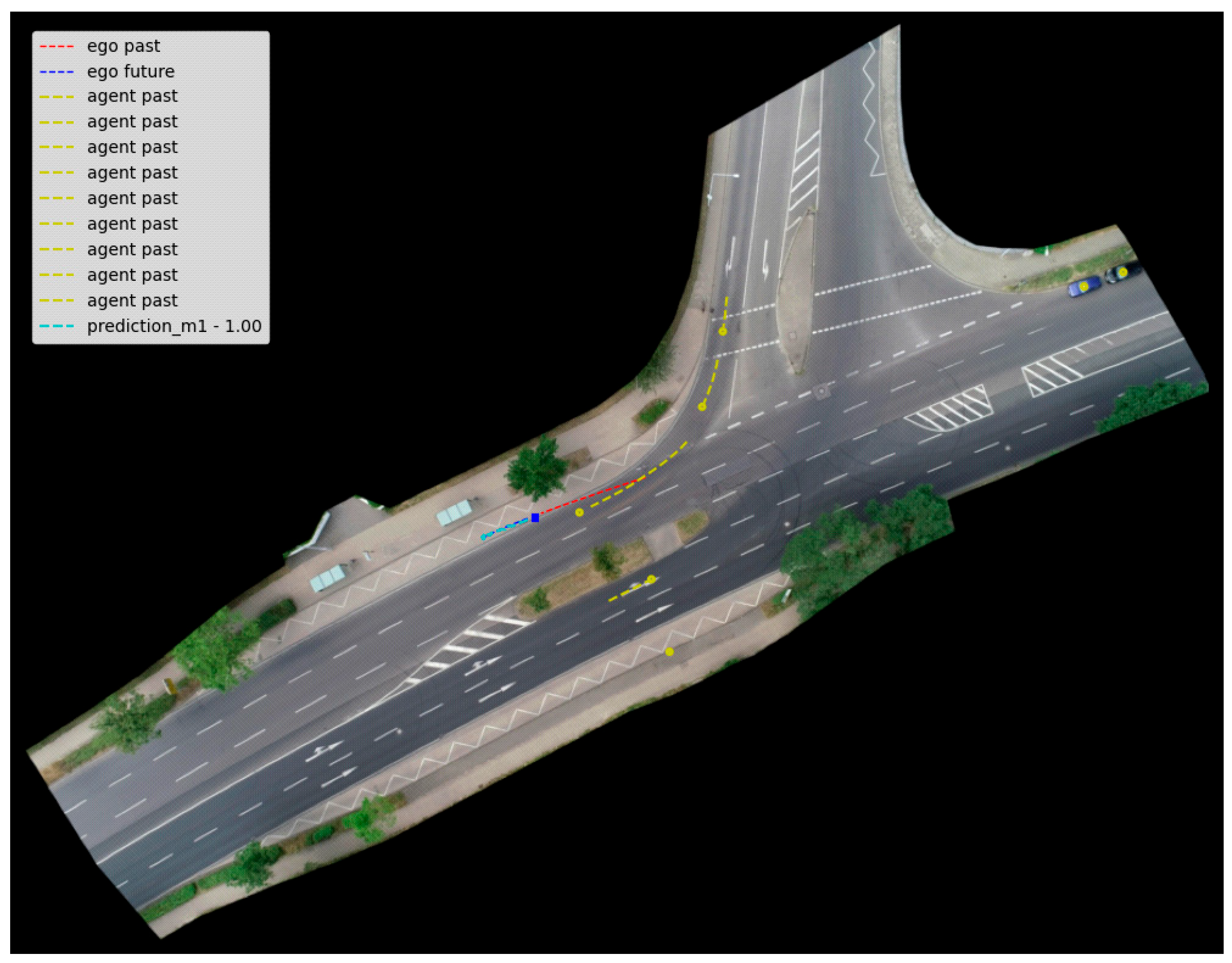
Figure 12, some results are displayed using the unimodal approach when the current agent type is a car. Then, we show some predictions when the current agent type is a bus (
Figure 13), a bicyclist (
Figure 14), and a pedestrian (
Figure 15). The past trajectory of the ego agent is drawn in red, the desired trajectory is drawn in blue, and the predicted trajectory is drawn with light blue. The surrounding agents are represented in blue and yellow. These color codes are the same for all unimodal scenarios.
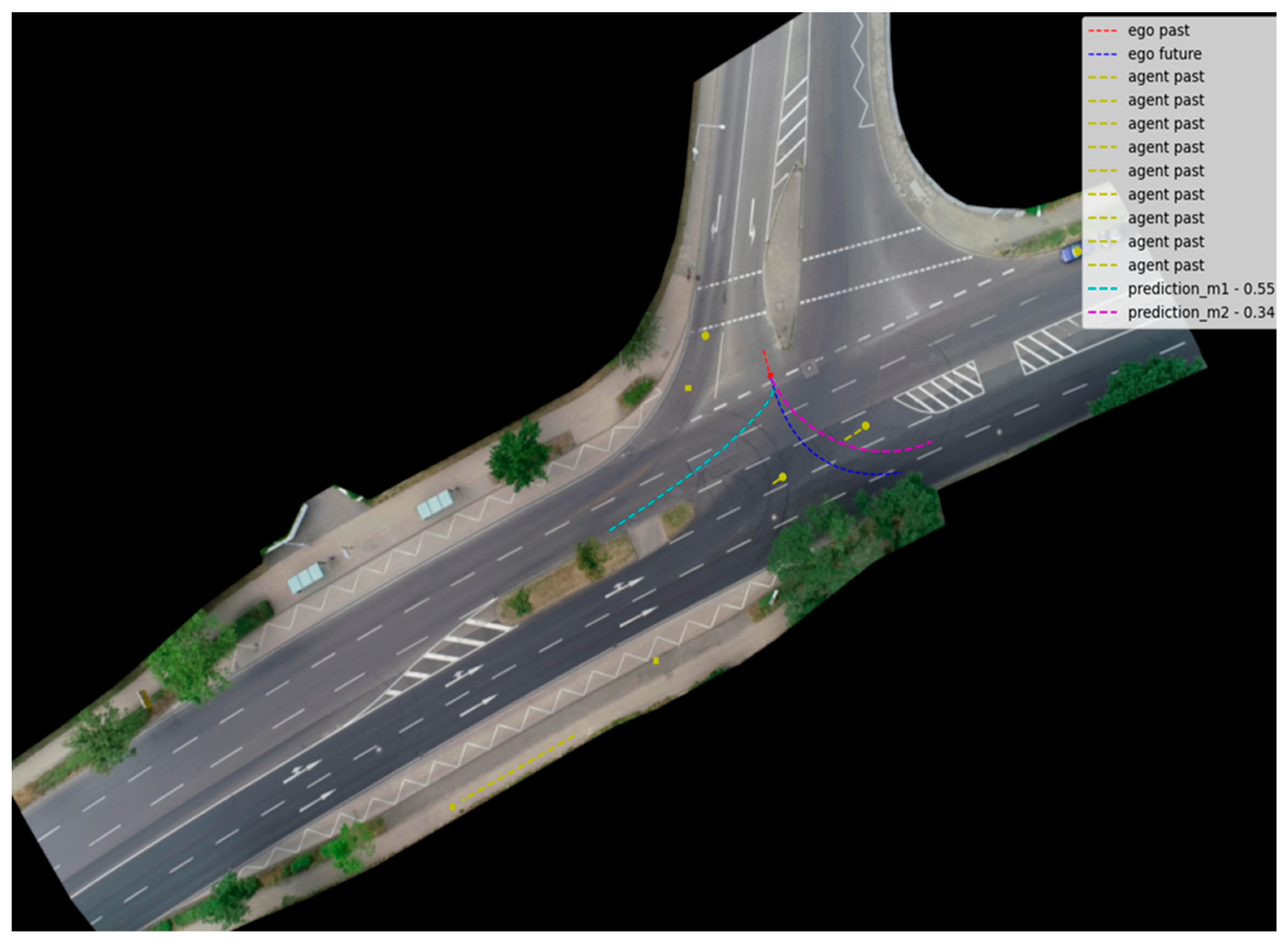
Similar results are presented as follows, this time considering the multimodal prediction. In these scenarios, the predicted trajectory is drawn with light blue, magenta, and green. The current agent types are a car (
Figure 16) and a bicyclist (
Figure 17).
5.2.3. Decreasing the Number of Predicted Points
An idea for a faster prediction of future trajectories for different traffic participants is to reduce the number of predicted points and to interpolate the values in order to obtain the entire trajectory. This can be observed in
Figure 18.
Table 5 contains the results corresponding to fewer predicted points for cars with the unimodal approach.
5.2.4. Comparison with Other Models
In this section, we include some results obtained in recent years (2021–2023) by other researchers using various methods on the inD dataset.
Table 6,
Table 7 and
Table 8 organize the results by paper, subset of the database used (e.g., certain intersections), and by model type. The same metrics (ADE and FDE) are considered. When a paper reports multiple results for a certain class of scenarios, only the best ones are included in
Table 6,
Table 7 and
Table 8, i.e., the best results rather than the average results are selected. It is important to note that the data refer to the trajectory prediction for all vehicles, while our approach also takes into account the type of traffic participants for prediction.
It should be noted that these values should not be directly compared, as different authors use different parts of the inD dataset, different prediction horizons, or even certain predefined data splits to test the models’ prediction capabilities. Therefore, a comparison with the results reported in the previous section should be considered from a qualitative point of view. Nevertheless, evaluating different methods for the same dataset can provide the reader with a general idea of the order of magnitude of the obtained errors.
There are other authors who focus only on trajectory prediction for pedestrians, e.g., [
34], which uses the general inD dataset. The results are displayed in
Table 9.
Upon analysis of the values presented by these authors, we observe that our results are comparable, and even better, in the unimodal case. However, it should be emphasized that our main goal was not solely to minimize some metric, but to create a model that can feasibly run in a real autonomous car. Due to real-time constraints, we were unable to explore more computationally expensive methods that may have resulted in lower errors. Nonetheless, we believe that the prediction quality obtained by our proposed model is on a par with other complex techniques that contribute to the current state of the art.
5.3. Vehicle Integration within the PRORETA 5 Project
A separate dataset was created for vehicle integration, as no dataset was available that matched the specific scenarios required by the project. For this reason, the dataset was created based on real measurements from the vehicle and by using the CARLA simulator [
43] with QGIS [
44] with the same interfaces as in the real vehicle. The simulated scenarios were created to have more variation in the dataset.
The network models were developed using the PyTorch framework in Python. The trained networks were then exported in the ONNX (Open Neural Network Exchange) format and imported for use with the C language on the car computer.
By using the Frenet coordinate system, the reference path was considered to be the center of the road. This was extracted with a converter from a measurement as we can see in
Figure 19. This is the test track that was used to develop the solution in the PRORETA 5 project.
Beside the difficulties arising from the fact that there were not enough data available for training, another challenge was to synchronize the module with the other modules running on the vehicle. In this case, the prediction approach was implemented to have two options, one to be input-triggered and the other one to be time-triggered (once every 100 ms). For the input-triggered concept, which was eventually used, the prediction module is triggered by the perception module which has a variable frequency of sending output data. Since the prediction must provide a predicted trajectory with a fixed timestamp, in our case 0.2 s, time synchronization is necessary. In order to accomplish this, an additional interpolation module was implemented.
Another important aspect is to check whether a predicted trajectory is valid or not, e.g., if some points are off road or if the distance between the current position and the first predicted point is too large. If it is not valid, it should be replaced by a backup trajectory that is computed based on the specific situation. This is important to ensure a valid output in a real vehicle and to improve the planned trajectory of the ego vehicle that takes into account the predicted trajectories of the other traffic participants.
In
Figure 20, one can see some results from the real vehicle that include the planned trajectory of the ego vehicle and the predicted trajectory of the other agents.
6. Conclusions
In this paper, we propose a method for predicting the trajectories of various types of traffic participants using vectors and an original design of a neural network. This technique was developed using the inD dataset and a dataset created from real-world scenarios. One of the main advantages of this approach is that it is integrated and can be run on a real vehicle.
An important aspect of this research was the dataset used to develop and train the model. In this particular case, vectors were necessary, as opposed to images, because the information from the sensors was assumed to have already been created. Another challenge was that most of the available vector datasets did not match the scenarios required for the project. After studying and implementing various vector approaches, we discovered that some of them did not produce the desired results. This makes a fair comparison between the presented method and other methods difficult to achieve.
The paper shows that the unimodal implementation performs better than the multimodal implementation because most maneuvers follow the lane, and, therefore, many variations in the trajectories cannot be learned. In the case of bicyclists, there are more variations, resulting in better results.
We included many practical details about using prediction in a real-world case, providing a more hands-on approach to the topic. This level of detail is often omitted in other papers, but we have found that different approaches to handling these details can have a significant impact on the overall performance of prediction.
Our method takes into account the constraints related to real-time operation in an actual self-driving car, ensuring that the predictions made are feasible and relevant in a practical setting. Synchronization with other modules, such as the perception and trajectory planning module, is crucial for a successful implementation of this technique.
As future research directions, this method can be extended to newer vector-based datasets and can be applied to other time series, further increasing its scope and potential impact in the field. An additional parameter can be added to measure the level of noise and variation in the data for the multimodal case, in order to create a balance between trying to fit data to a conservative trajectory or allowing several different trajectories to be generated. This would provide a more comprehensive understanding of the data and its reliability, allowing for more informed predictions. An explicit analysis of the uncertainty of predictions is another valuable area for further investigation. This analysis can provide insight into the confidence level of the predictions made by the model and allow for a better understanding of its limitations. It can improve the reliability of the predictions and increase the confidence in the system.


