Optimal Orientation of Solar Panels for Multi-Apartment Buildings

Abstract

In this paper, we present a mathematical algorithm for the optimal orientation of solar panels for multi-apartment buildings. Currently, photovoltaic power generation has increasingly become an effective method. It has the advantage of not causing environmental pollution; however, it has the disadvantage of relatively low power generation efficiency. To increase the power efficiency of the panel, one can consider a rotation. However, if there is a limitation to the rotation angle of the solar panel, especially in multi-apartment buildings, it is desirable to install the panel at the optimal angle under given constraints. Therefore, we present a simple and practical method to evaluate the optimal installation angle of the panel. Using the proposed method, it is easy to find an optimal installation angle to achieve the best power generation efficiency based on the latitude and azimuth angles. To demonstrate the effectiveness of the proposed algorithm, several numerical simulation results are provided.

1. Introduction

Solar energy is one of the important energy sources, and many countries, therefore, have realized the important role of renewable energies due to the depletion of conventional energy sources [1,2]. In particular, interest in solar power generation is increasing due to the dangers of nuclear/thermal power generation that have recently occurred in several countries. The advantages of using solar power generation are as follows. First, because it uses solar energy, it does not require fuel costs and is a clean energy source that does not generate air pollution or waste. Second, because the power generation unit is composed of semiconductor devices, there is no vibration and noise, and automation is easy. Lastly, efficient power generation is possible because power can be maximized during the daytime and summer when the power load is high.

However, photovoltaic power generation has several problems. First, there is a time constraint on energy generation. This is a very important issue and inevitably causes the problem of maximum efficiency and storage capacity in a limited time. Second, the profitability is not good due to the high unit price for power generation. For example, it is about 4 to 5 times more expensive than nuclear power generation.

In everyday life, one can often see solar panels installed in multi-apartment buildings to generate solar energy, as shown in Figure 1. An installation angle of the solar panel is important to collect photons efficiently [3]. If the solar panels are installed in a parallel direction to the building, then the energy efficiency is usually not optimal at each location. Therefore, we propose a simple mathematical algorithm for setting the angle and direction of the solar panel that can produce the maximum solar energy efficiency at each location based on the latitude and azimuth angle under several constraints.

Figure 1. (a) The actual solar panel installed in the apartment. (b) An enlarged view.

As there is a lot of interest in solar panels and photon collectors around the world, many researchers have investigated calculating their optimal tilt angles [4,5,6,7,8,9,10,11,12,13,14,15,16,17,18]. Not only the optimal angle calculation but also the research on factors that can affect the performance of solar panels such as wind speed [19], weather [20], latitude and longitude [21] are in progress. In South Africa, the authors in [5] calculated the annual solar insolation for all possible angles on fixed collectors using the data obtained from the nine measuring stations. Other studies proposed using incident beam radiation-based maximization approach [6], a latitude-based optimization approach in the Mediterranean region [7], and non-linear time-varying particle swarm optimization in Taiwan [8].

As most researchers have reported that the maximum power can be harvested when a solar panel is equipped with a sun-tracking system. Referred researches suggest that the different adjustment number of intervals from 4 to 12 to obtain maximum energy in each country: 8 times a year in Iraq [10], 12 times a year in Syria [11], and also 12 times a year but each month adjusting the tilt angle which can achieve 8% more surface radiation compared with yearly adjustment in Saudi Arabia [12]. Furthermore, the solar panel with a fixed tilt angle without representing the number of yearly adjustments got 10–25% higher irradiations with increasing latitude in USA [13], the variation of optimal tilt angle throughout a year is between $0^{\circ }$ and ${65}^{\circ }$ in Turkey [14].

In [16], the authors present several models to calculate the optimal slope of the solar panel accurately at any location in the world. Using the proposed models, the authors estimate the annual energy output along with the amount of irradiance stored per hour according to the slope of the solar panel. There is a study that calculates the optimal tilt angle of a solar panel using machine learning recently [17]. In this study, energy generation simulations of panels are performed to calculate monthly and yearly panel angles, and economic cost effects are also evaluated in real-world environments. In [18], the optimal solar panel angle is calculated for the maximum energy yield. Calculating the cosine effect of the angle of the sun and the angle of the panel, the authors present a permanent fixed optimal angle but also a four-season or monthly adjustment to improve the total annual solar energy yield. In [22], the authors investigate the arrangement of solar panels for various spaces. Solar panels can be arranged to maximize energy production in limited spaces such as rooftops of buildings. The results suggest that the suitable deployment of solar panels could increase energy production by up to 6%. In [23], the authors introduce a new term, the tolerance angle. The tolerance angles refer to the angular range of optimal solar panels that minimize economic losses. It can be useful during actually installing solar panels.

The main purpose of this paper is to present a mathematical algorithm for the optimal orientation of solar panels for multi-apartment buildings under several constraints. Let $\mathbf{m}$ and $\mathbf{n}$ be the representative of the solar beam and normal vector of the panel, respectively. Then, we consider the following optimizing problem

$$\begin{array}{c}\hfill \underset{\mathbf{n}}{arg\; min}{\parallel \mathbf{m}-\mathbf{n}\parallel }_2,\end{array}$$

(1)

when the solar vector $\mathbf{m}$ and certain constraint for $\mathbf{n}$ is given.

The outline of this paper is as follows. A mathematical model for finding the optimal position of a solar panel for buildings is described in Section 2. Numerical results are listed in Section 3. We finalize the paper with the conclusion in Section 4. A code implementation is included in Appendix A for users who may not be familiar with the content.

2. Mathematical Modeling

In this section, we propose our mathematical modeling to derive the optimal orientation of solar panels under several constraints. First, we consider a rectangular panel $OABC$ (represented dark gray) whose horizontal and vertical lengths are $L_y$ and $L_z$, respectively, as shown in Figure 2.

Figure 2. Schematic illustrations of our mathematical modeling to the rotated panel, (a) fixing A and (b) fixing B.

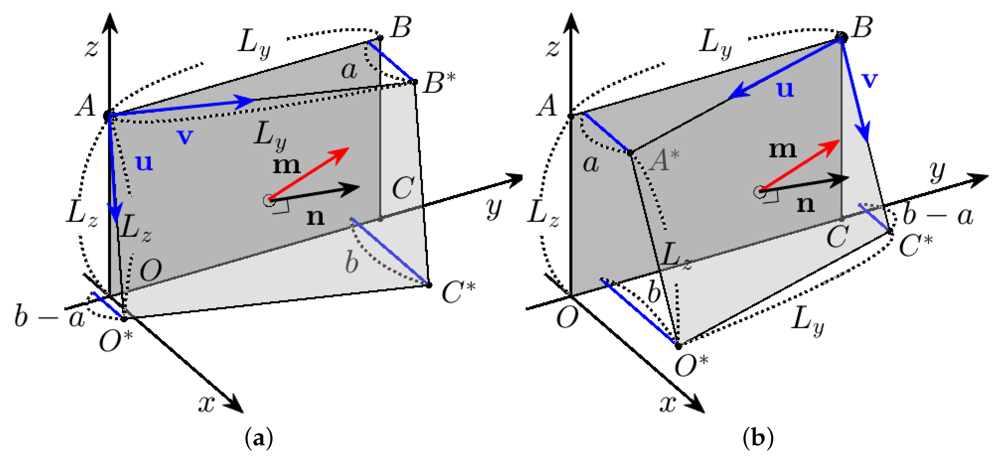
As shown in Figure 2a, we suppose that the panel $OABC$ is on $yz$-plane and the coordinates of $A,B$, and C are determined automatically. Then, we move the solar panel while keeping the coordinate of $A(0,0,L_z)$ fixed. Moreover, we fix the height of panel $L_z$. We then obtain a moved solar panel $A{B}^{*}{C}^{*}{O}^{*}$, which is represented by light gray. Here, let a and b be the lengths of the perpendicularity from $B^{*}$ and $C^{*}$ to the plane $OABC$, respectively. We can know that the length of the perpendicularity from $O^{*}$ to $OABC$ is $b-a$. Note that the foot perpendicular on the plane $OABC$ from $B^{*}$ is a point on the plane, not B. Similarly, it is important to know that each foot perpendicular on the plane $OABC$ from $O^{*}$ and $C^{*}$ is also a point on the plane. By using the Pythagorean theorem, we can obtain the coordinate of $B^{*}$ as $(a,\sqrt{L_y^2-a^2},L_z)$. However, we only obtain the x-coordinate of $C^{*}$ as b. In this case, we define the coordinate of $C^{*}$ as $(b,y,z)$, in which y and z are unknown constants. The purpose of our modeling is to find the best-fitted normal vector of the plane $A{B}^{*}{C}^{*}{O}^{*}$ to a given sunlight vector. In other words, finding $(a,b,y,z)$ is our primary goal. In our modeling, we can get the two equations from the geometry. The first equation is obtained from the fact that the length of $A{C}^{*}$ equals the diagonal of a rectangular panel. That is,

$$\begin{array}{c}\hfill b^2+y^2+{(z-L_z)}^2=L_y^2+L_z^2.\end{array}$$

(2)

Moreover, we know that the length of $B^{*}{C}^{*}$ is equal to the height of the panel, $L_z$, we have the following

$$\begin{array}{c}\hfill {(a-b)}^2+{\left(\sqrt{L_y^2-a^2}-y\right)}^2+{(L_z-z)}^2=L_z^2.\end{array}$$

(3)

Then, we can combine the two Equations (2) and (3) to get y and z in terms of a, b, $L_y$, and $L_z$ as follows:

$$\begin{array}{c}\hfill y=\frac{L_y^2-ab}{\sqrt{L_y^2-a^2}},z=L_z-\sqrt{L_y^2+L_z^2-b^2-y^2}.\end{array}$$

(4)

Now, we get $O^{*}=(b-a,y-\sqrt{L_y^2-a^2},z)$ from the fact that it shares the midpoint of the rectangle ($O^{*}+B^{*}=A+C^{*}$). To find the normal vector $\mathbf{n}$ of plane $A{B}^{*}{C}^{*}{O}^{*}$, we define both vectors $\mathbf{u}$ and $\mathbf{v}$ using $A,O^{*}$, and $B^{*}$. By using the cross product of $\mathbf{u}$ and $\mathbf{v}$, we can find the normal vector $\mathbf{n}$ as follows:

$$\begin{array}{c}\hfill \mathbf{n}=\frac{\left((L_z-z)\sqrt{L_y^2-a^2},a(z-L_z),b\sqrt{L_y^2-a^2}-ay\right)}{L_y{L}_z}.\end{array}$$

(5)

Similarly, we consider the case in which B is fixed as shown in Figure 2b. Following the above method, we can obtain the specific coordinates of $O^{*},A^{*},$ and $C^{*}$, which are moved points from $O,A,$ and C, respectively. To sum up, let us assume that the coordinates $O,A,B,$ and C are given as follows:

$$\begin{array}{c}\hfill O=(0,0,0),A=(0,0,L_z),B=(0,L_y,L_z),C=(0,L_y,0).\end{array}$$

(6)

For the cases (i) fixed A and (ii) fixed B, we can derive the remaining coordinates of the panel as follows:

$$\begin{array}{cc}\hfill \left(\mathrm{i}\right)O^{*}& =(b-a,y-\sqrt{L_y^2-a^2},z),B^{*}=(a,\sqrt{L_y^2-a^2},L_z),C^{*}=(b,y,z),\hfill \end{array}$$

(7)

$$\begin{array}{cc}\hfill \left(\mathrm{ii}\right)O^{*}& =(b,L_y-y,z),A^{*}=(a,L_y-\sqrt{L_y^2-a^2},L_z),C^{*}=(b-a,L_y-y+\sqrt{L_y^2-a^2},z).\hfill \end{array}$$

(8)

Subsequently, we need to evaluate the normal vector of the panel. In multi-apartment buildings, if an inclination angle is formed between the panel and the bottom plane perpendicular to the wall where the panel is installed less than a certain degree, it can be a nuisance downstairs due to a shade from the panel. For this reason, the angle is restricted by regulation, and we take a threshold as $\pi /3$ in this paper. Therefore, we can set the maximum value of b to $L_z/2$; hence we have the constraint $0\le a\le b\le L_z/2$ for the problem (1). Figure 3a shows the curved triangular region where all the possible normal vectors can be located. Note that we set $L_z=1$ for simplicity.

Figure 3. (a) All the possibilities of normal vector can be located. It is a curved triangular shape. Note that the black part corresponds to Figure 2a, and the blue part corresponds to Figure 2b. (b) Schematic illustration of finding the nearest normal vector $\mathbf{n}$, which is represented by green color, using the projection of solar beam $\mathbf{m}$, which is represented by red color, to the plane generated by any two vectors, $\mathbf{p}$ and $\mathbf{q}$, such that lie on the nearest boundary of the region to $\mathbf{m}$. Note that we normalize the magnitude of the normal vector.

There are two cases for the given vector representing a solar beam $\mathbf{m}$. One is in the curved triangular region, and the other is outside of the curved region. We just take $\mathbf{n}=\mathbf{m}$ to the former. However, one cannot take a normal vector that coincides with $\mathbf{m}$ if $\mathbf{m}$ is outside of the region. In this case, we have to choose $\mathbf{n}$ such that $\mathbf{m}·\mathbf{n}$ is maximized. Such a vector can be found as normalizing the vector, which is given by the projection of $\mathbf{m}$ to the plane generated by any two vectors that lie on the nearest boundary of the region to $\mathbf{m}$. Figure 3b depicts the process of how to find the corresponding fitted normal vector to $\mathbf{m}$.

To be more precise, we can obtain the normal vector $\mathbf{n}$ as follows:

$$\begin{array}{c}\hfill \mathbf{n}=\frac{\parallel {\mathbf{n}}_1{\parallel }^2\mathbf{m}-(\mathbf{m}·{\mathbf{n}}_1){\mathbf{n}}_1}{\parallel \parallel {\mathbf{n}}_1{\parallel }^2\mathbf{m}-(\mathbf{m}·{\mathbf{n}}_1){\mathbf{n}}_1\parallel },\end{array}$$

(9)

where ${\mathbf{n}}_1=\mathbf{p}\times \mathbf{q}$. An important thing is that we can simplify the representation of boundary vectors as the relation between a and b. Three endpoints of the triangular boundary are expressed by (i) $a=0$, $b=L_z/2$, (ii) $a=b$, $b=L_z/2$ where A is fixed, (iii) $a=b$, $b=L_z/2$ where B is fixed. Thus, one can easily get the best-fitted orientation for the solar panel by following the above process.

The solar beam $\mathbf{m}$ is treated as a given constant throughout the whole process so far. The only remaining thing is, therefore, to choose an appropriate representative $\mathbf{m}$. One way to find the representative of a solar beam is by applying the mean value property to the trace of the sun. Assume that Earth is a sphere, and the orbit of Earth is a circle. Then the azimuth can be computed. Considering the spherical coordinates system while looking at the celestial body from the current position. Note that we fix the current position as Seoul, whose latitude is approximately $37.{5326}^{\circ }$. The south meridian altitude of the sun is on a great circle of spheres when the celestial body passes through the meridian of Earth. Furthermore, there are two times when the orbit of Earth and its axis of rotation are perpendicular; we call this vernal/autumnal equinox, respectively. Moreover, summer and winter solstices are parallel to the equinox. Therefore, the procedure assumes that the values between the maximum and minimum south meridian altitude have the same normal vector. To depict it clearly, we present Figure 4a as follows.

Figure 4. (a) Illustration of the trajectory of the sun when the positions of Earth are on solstice and equinox in Seoul. Note that these three traces have an identical normal vector. (b) Illustration of a trace of the sun (magenta) and possibly generating trajectory (solid line). Note that the dotted line is part of the trace where the sunlight does not shine due to the azimuth angle of buildings. Solar vector (red) and solar panel (blue) are represented with the shaded region, which represents a possible area to receive sunlight. The black cuboid is a schematic illustration of the residence; it is actually treated as a point (the origin) in our method. (c) Illustration of the solar vector (red) and the best-fitted normal vector (blue). Note that a cyan-colored triangle represents the boundary of all possibly taken normal vectors of the solar panel.

Because the normal vectors of solstice and equinox are identical, we can easily find the trajectory of average solar movement via the intersection curve with this unique normal vector. Then we can compute $\mathbf{m}$ if we know the azimuth angle of the place to install the solar panel. Suppose that we wish to install the panel in the building to a certain degree. Figure 4b depicts a trace of solar movement and the corresponding representative solar vector.

Therefore, combining all of the above conditions, we can find the best-fitted vector out of all the normal vectors that the solar panel can take along with respect to the solar vector. Figure 4c shows the evaluated solar vector and the derived best-fitted normal vector corresponding to the solar vector.

In summary, the optimal solar panel installation can be determined by knowing the south-middle altitude of the desired area and the azimuth angle of the building where the solar panel will be installed. Figure 5 depicts the procedure for finding the optimal installation specification of solar panels with respect to geometric features.

Figure 5. Schematic illustration to find the optimal installation specification of solar panels.

3. Numerical Simulation Results

We present several numerical simulation results in this section. We fix the solar panel specification as $L_y=3$ and $L_z=2$ because this is the common length ratio of the standard solar panel. To evaluate the solar elevation angle $\alpha$ at noon, we use the following formula [24].

$$\begin{array}{c}\hfill \alpha =arcsin(sin\varphi sin\delta +cos\varphi cos\delta ),\end{array}$$

(10)

where $\varphi$ is the latitude, and $\delta$ is the declination angle defined as

$$\begin{array}{c}\hfill \delta =arcsin\left(-sin\mathrm{\Theta }cos\left(\frac{2\pi (d+10)}{365.24}+0.0334sin\left(\frac{2\pi (d-2)}{365.24}\right)\right)\right),\end{array}$$

(11)

where $\mathrm{\Theta }\approx 23.{44}^{\circ }$ is degree of the rotation axis of Earth, and d represents the number of days since January 1st in 2022. For instance, one can take $d=3+9/24$ for 09:00 A.M. on 4 January 2022. Note that this approximation formula is fitted to UTC + 00:00. Though there is a slight difference (up to the second decimal place) between the fixed and local time-based formula, this condition can be ignored because we consider the declination angle only up to the first decimal place. All the latitudes are sourced from [25]. Table 1 shows monthly installation specification data with respect to the monthly arithmetic average of the south altitude of each city with the azimuth angle $73\pi /72$ from the north. Note that we use the notation $(a,b,y,z)$ to represent the computed parameters hereafter.

Table 1. Installation specification with respect to the south meridian altitude of each city. The azimuth angle is $73\pi /72$. Note that the data is aligned by month from the top (January) to the bottom (December).

City	Seoul	Ottawa	Dublin
$(a,b,y,z)$	$(0.0006,1,2.9998,0.2677)$	$(0.1309,0.9244,2.8540,0.1665)$	$(0.1309,0.6668,2.9250,0.0739)$
	$(0,1,3,0.2679)$	$(0,1,3,0.2679)$	$(0.1309,0.9270,2.8532,0.1677)$
	$(0,1,3,0.2679)$	$(0,1,3,0.2679)$	$(0,1,3,0.2679)$
	$(0,1,3,0.2679)$	$(0,1,3,0.2679)$	$(0,1,3,0.2679)$
	$(0,1,3,0.2679)$	$(0,1,3,0.2679)$	$(0,1,3,0.2679)$
	$(0,1,3,0.2679)$	$(0,1,3,0.2679)$	$(0,1,3,0.2679)$
	$(0,1,3,0.2679)$	$(0,1,3,0.2679)$	$(0,1,3,0.2679)$
	$(0,1,3,0.2679)$	$(0,1,3,0.2679)$	$(0,1,3,0.2679)$
	$(0,1,3,0.2679)$	$(0,1,3,0.2679)$	$(0,1,3,0.2679)$
	$(0,1,3,0.2679)$	$(0,1,3,0.2679)$	$(0.0999,1,2.9684,0.2275)$
	$(0,1,3,0.2679)$	$(0.1309,1,2.8271,0.2037)$	$(0.1309,0.7508,2.9045,0.0996)$
	$(0.0631,1,2.9796,0.2423)$	$(0.1309,0.8553,2.8755,0.1376)$	$(0.1309,0.5941,2.9406,0.0549)$

Next, we present Table 2, a monthly installation specification data with respect to the monthly arithmetic average of the south altitude of each city with the azimuth angle $35\pi /36$ from the north.

Table 2. Installation specification with respect to the south meridian altitude of each city. The azimuth angle is $35\pi /36$. Note that the data is aligned by month from the top (January) to the bottom (December).

City	Wellington	Copenhagen	Paris
$(a,b,y,z)$	$(0,1,3,0.2679)$	$(0.2615,0.7166,2.9132,0.0536)$	$(0.2615,0.9395,2.8491,0.1219)$
	$(0,1,3,0.2679)$	$(0.2615,0.9775,2.8363,0.1367)$	$(0.1356,1,2.9578,0.2133)$
	$(0,1,3,0.2679)$	$(0,1,3,0.2679)$	$(0,1,3,0.2679)$
	$(0,1,3,0.2679)$	$(0,1,3,0.2679)$	$(0,1,3,0.2679)$
	$(0.0882,1,2.9719,0.2322)$	$(0,1,3,0.2679)$	$(0,1,3,0.2679)$
	$(0.2035,1,2.9389,0.1866)$	$(0,1,3,0.2679)$	$(0,1,3,0.2679)$
	$(0.1574,1,2.9516,0.2046)$	$(0,1,3,0.2679)$	$(0,1,3,0.2679)$
	$(0,1,3,0.2679)$	$(0,1,3,0.2679)$	$(0,1,3,0.2679)$
	$(0,1,3,0.2679)$	$(0,1,3,0.2679)$	$(0,1,3,0.2679)$
	$(0,1,3,0.2679)$	$(0.2031,1,2.9391,0.1868)$	$(0.0129,1,2.9957,0.2627)$
	$(0,1,3,0.2679)$	$(0.2615,0.8008,2.8912,0.0759)$	$(0.2615,1,2.8213,0.1542)$
	$(0,1,3,0.2679)$	$(0.2615,0.6438,2.9301,0.0376)$	$(0.2615,0.8695,2.8712,0.0972)$

Subsequently, we present Table 3, which represents optimal installation specification data with respect to the monthly average of the south altitude of each city with the azimuth angle $17\pi /18$.

Table 3. Installation specification with respect to the south meridian altitude of each city. The azimuth angle is $17\pi /18$. Note that the data is aligned by month from the top (January) to the bottom (December).

City	Rome	Moscow	Riyadh
$(a,b,y,z)$	$(0.2391,1,2.9296,0.1730)$	$(0.5209,0.9653,2.8404,0.0530)$	$(0,1,3,0.2679)$
	$(0.0021,1,2.9993,0.2671)$	$(0.3910,1,2.8944,0.1180)$	$(0,1,3,0.2679)$
	$(0,1,3,0.2679)$	$(0.0199,1,2.9934,0.2598)$	$(0,1,3,0.2679)$
	$(0,1,3,0.2679)$	$(0,1,3,0.2679)$	$(0,1,3,0.2679)$
	$(0,1,3,0.2679)$	$(0,1,3,0.2679)$	$(0,1,3,0.2679)$
	$(0,1,3,0.2679)$	$(0,1,3,0.2679)$	$(0,1,3,0.2679)$
	$(0,1,3,0.2679)$	$(0,1,3,0.2679)$	$(0,1,3,0.2679)$
	$(0,1,3,0.2679)$	$(0,1,3,0.2679)$	$(0,1,3,0.2679)$
	$(0,1,3,0.2679)$	$(0,1,3,0.2679)$	$(0,1,3,0.2679)$
	$(0,1,3,0.2679)$	$(0.2798,1,2.9195,0.1577)$	$(0,1,3,0.2679)$
	$(0.1694,1,2.9482,0.1999)$	$(0.5209,1,2.8113,0.0752)$	$(0,1,3,0.2679)$
	$(0.2969,1,2.9154,0.1514)$	$(0.5209,0.8942,2.8636,0.0371)$	$(0,1,3,0.2679)$

According to the above tables, it can be verified that the rate of change of the parameter $(a,b,y,z)$ is nearly zero when the south meridian altitude is high, and the latitude is low. These results are independent of the azimuth angle of buildings. Because time series data can be generated, it would be better to rotate the panel in real-time; however, in the case of installing a solar panel in a residential area, it is expensive to construct the panel support that moves according to the time. Therefore, we employ a weighted mean of monthly $(a,b,y,z)$ based on daylight time. More precisely, we adopt the following weight formula to each monthly weight $w_i$ as   

$$\begin{array}{c}\hfill w_i=\frac{l_i}{{\sum }_{i=1}^{12}{l}_i},i=1,\dots ,12,\end{array}$$

(12)

where $l_i$ represents the length of the trajectory of the sun for the i-th month. Figure 6, Figure 7 and Figure 8 represent the weighted average values of the south meridian altitude in selected regions and those of parameters $(a,b,y,z)$.

Figure 6. Weighted average values of parameters $(a,b,y,z)$ with respect to each region in Table 1. Note that the number displayed after the city is the weighted average value of the south meridian altitude.

Figure 7. Weighted average values of parameters $(a,b,y,z)$ with respect to each region in Table 2. Note that the number displayed after the city is the weighted average value of the south meridian altitude.

Figure 8. Weighted average values of parameters $(a,b,y,z)$ with respect to each region in Table 3. Note that the number displayed after the city is the weighted average value of the south meridian altitude.

In addition, we evaluate the energy efficiency compared to the panel installed in parallel to its support by using the following function,

$$\begin{array}{c}\hfill E(\mathbf{n};\mathbf{m},{\mathbf{n}}_0)=\sum _{i=1}^{12}{D}_i\mathbf{m}·({\mathbf{n}}_i-{\mathbf{n}}_0)\times 100(\%),\end{array}$$

(13)

where $D_i$ is given constant and ${\mathbf{n}}_0$ represents a normal vector of the panel installed in parallel to its support. Table 4 shows the annual efficiency based on (13) for each city.

Table 4. The annual energy efficiency based on (13) for each city. The azimuth angle is (a) $73\pi /72$, (b) $35\pi /36$, (c) $17\pi /18$.

(a)	Seoul	Ottawa	New Delhi	Dublin	Brasilia
Efficiency (%)	$12.6241$	$9.7297$	$15.7840$	$7.1309$	$18.9755$
(b)	Kuala Lumpur	Wellington	Paris	Copenhagen	Asuncion
Efficiency (%)	$20.1175$	$11.0114$	$8.5754$	$6.5555$	$16.558$
(c)	Jakarta	Buenos Aires	Rome	Moscow	Riyadh
Efficiency (%)	$19.0135$	$13.1064$	$10.9335$	$6.8133$	$16.2883$

From the above results, it is effective to set the installation angle of the solar panel using the proposed method. In particular, the reason why the efficiency is higher in the area near the equator is that the south meridian altitude is much higher than in other areas.

4. Conclusions

In this paper, we propose a simple mathematical method to obtain the optimal installation conditions for solar panels in multi-apartment buildings. The presented method provides optimal installation information by considering the azimuth of the building and the amount of sunlight (per month). Through the numerical simulation results, we can confirm that more efficient energy generation can be expected via our method than the panel simply fixed on support without rotation (parallel to the building). Note that the efficiency is maximized if the panel can be rotated in real-time; however, it is not practical for residence; hence, finding an optimal fixed position for the panel is essential to have maximal efficiency under several constraints. In this study, the shadow effect (caused by itself or any other buildings) and the diffuse and reflected irradiations are not considered in the proposed method. These effects are common in urban areas; therefore, we plan to address these aspects in future works.