New Approaches on Parameter Estimation of the Gamma Distribution

Abstract

This paper discusses new approaches to parameter estimation of gamma distribution based on representative points. In the first part, the existence and uniqueness of gamma mean squared error representative points (MSE-RPs) are discussed theoretically. In the second part, by comparing three types of representative points, we show that gamma MSE-RPs perform well in parameter estimation and simulation. The last part proposes a new Harrel–Davis sample standardization technique. Simulation studies reveal that the standardized samples can be used to improve estimation performance or generate MSE-RPs. In addition, a real data analysis illustrates that the proposed technique yields efficient estimates for gamma parameters.

1. Introduction

The term representative points (RPs) indicates a set of supporting points with corresponding probabilities, which can be used as the best approximation of a d-dimensional probability distribution. Representative points can be regarded as a discretization of a continuous distribution, and are expected to retain as much information as possible. In the univariate case, X is considered to be a population random variable with cumulative distribution function (cdf) $F\left(x\right)$, a discrete random variable Z is defined to approximate X with probability mass function (pmf) by a set of supporting points $z=\{z_1,z_2,\cdots ,z_k\}$ ($-\infty <z_1<z_2<\cdots <z_k<\infty$) with probabilities $\{p_1,p_2,\cdots ,p_k\}$, where $P(Z=z_i)=p_i$ and ${\sum }_{i=1}^k{p}_i=1$. In the literature, there are several approaches to choosing the supporting point set z. For example, a set of random samples from $F\left(x\right)$ can be viewed as a representative of the distribution; Fang and Wang [1] suggest generating representative points based on the number theoretic method. In 1957, Cox [2] proposes the idea of using mean squared error (MSE) to measure the loss of information from $F\left(x\right)$, where

$$\begin{array}{c}\hfill MSE\left(z\right)=MSE(z_1,z_2,\cdots ,z_k)=E\left(\underset{i=1,\cdots ,k}{min}{(z_i-X)}^2\right)={\int }_{-\infty }^{\infty }\underset{i=1,\cdots ,k}{min}{(z_i-X)}^{2}dF\left(x\right).\end{array}$$

(1)

The point set $z^{MSE}=\{z_1^{MSE},\cdots ,z_k^{MSE}\}$ such that $MSE\left(z\right)$ arrives its minimum is called the mean squared error representative points (MSE-RPs) of $F\left(x\right)$. MSE-RPs are found to have many good properties and have been applied in study fields such as signal compression (Gersho and Gray [3]), numerical integration computation (Pagès [4,5]), simulating stochastic differential equation (Gobet et al. [6]; El Amri et al. [7]), statistical simulation (Fang et al. [8], Fang et al. [9]) and clothing standard settings (Fang and He [10]; Flury [11]). To compute MSE-RPs for different distributions, effective numerical methods are proposed. Fang-He algorithm (Fang and He [10]) calculates MSE-RPs by solving a system of non-linear equations; Lloyd I algorithm (Lloyd [12]), LBG algorithm (Linde et al. [13]) and Competitive Learning Vector Quantization algorithm (Pagès [5]) obtain MSE-RPs by iterating a long training sequence of data; Tarpey’s self-consistency algorithm (Tarpey [14]) brings the idea of k-means algorithm for generating MSE-RPs; Chakraborty et al. [15] provides an accelerate algorithm using Newton’s method. When the number of MSE-RPs (k) is large, obtaining MSE-RPs becomes computationally intensive. Fang and He [10] presents some discussion on the optimum choice of k.

Recently, the use MSE-RPs properties for some distributions have been studied in detail, including normal distribution (Fang et al. [8]), mixed normal distribution (Fang et al. [9] and Li et al. [16]), arcsine distribution (Jiang et al. [17]) and exponential distribution (Xu et al. [18]). A general relationship between MSE-RPs and population distribution can be found in the work of Fei [19] and Fang et al. [9]. The study of the gamma distribution’s MSE-RPs (gamma MSE-RPs) can be traced back to Fu [20], which discusses the existence of gamma MSE-RPs and establishes an algorithm for computing these points. The gamma distribution is one of the most important distributions in statistics and probability theory, it is worth taking a closer look at gamma MSE-RPs and discovering their merits. The innovations of this paper are listed as follows:

• New theoretical results prove the uniqueness of gamma MSE-RPs;
• Gamma MSE-RPs are found to outperform other types of representative points in parameter estimation;
• A new standardization technique is proposed to improve the estimation performance of random samples from the gamma distribution.

Our discussion will focus on these three perspectives. Section 2 provides some preliminary knowledge of the gamma distribution and different types of representative points for readers to access our content easily. Section 3 gives some theoretical discussion on the existence and uniqueness of gamma MSE-RPs. An algorithm for generating gamma MSE-RPs is recommended. Section 4 compares the performance of three typical gamma representative points in parameter estimation and simulation. The results demonstrate that gamma MSE-RPs take advantage of other representative points in many scenarios. Section 5 introduces a new Harrel–Davis standardization technique. Simulation studies show that the standardized samples have better performances than random samples in estimation and can be used to generate gamma MSE-RPs. Section 6 provides a real clinical data analysis and illustrates that the standardization technique yields efficient estimates for gamma parameters.

2. Preliminaries

2.1. The Gamma Distribution and Gamma MSE-RPs

A gamma-distributed random variable with shape parameter a and rate parameter b is denoted $X\sim Gamma(a,b)\equiv Ga(a,b)$. The corresponding probability density function (pdf) in the shape-rate parametrization is

$$\begin{array}{c}\hfill f(x;a,b)=\frac{b^a}{\Gamma \left(a\right)}{x}^{a-1}{e}^{-bx},\mathrm{for}x>0,a,b>0,\end{array}$$

(2)

where $\Gamma (·)$ is the gamma function. The mean, variance, skewness and kurtosis of X are

$$\begin{array}{c}\hfill \mu =\frac{a}{b},{\sigma }^2=\frac{a}{b^2},\mathrm{Sk}\left(X\right)=\frac{2}{\sqrt{a}}\mathrm{and}\mathrm{Ku}\left(X\right)=\frac{6}{a}\end{array}$$

(3)

accordingly. Let $z^{MSE}=\{z_1^{MSE},z_2^{MSE},\cdots ,z_k^{MSE}\}$ be a set of MSE-RPs for $Ga(a,b)$, derive the following intervals

$$\begin{array}{c}\hfill \begin{array}{c}\hfill I_1=\left(0,\frac{z_1^{MSE}+z_2^{MSE}}{2}\right),I_2=\left[\frac{z_1^{MSE}+z_2^{MSE}}{2},\frac{z_2^{MSE}+z_3^{MSE}}{2}\right),\cdots ,\\ \hfill I_{k-1}=\left[\frac{z_{k-2}^{MSE}+z_{k-1}^{MSE}}{2},\frac{z_{k-1}^{MSE}+z_k^{MSE}}{2}\right),I_k=\left[\frac{z_{k-1}^{MSE}+z_k^{MSE}}{2},+\infty \right)\end{array}\end{array}$$

(4)

with the corresponding probabilities in these intervals as

$$\begin{array}{c}\hfill p_i={\int }_{I_i}f(x;a,b)dx,i=1,\cdots ,k.\end{array}$$

(5)

Here $f(x;a,b)$ is the pdf in (2).

2.2. Other Types of Representative Points

In addition to MSE-RPs, two other types of representative points are frequently discussed in the literature: Monte Carlo representative points and number theoretic representative points.

(A)

Monte Carlo representative points (MC-RPs)

MC-RPs are generated by the Monte Carlo method. Consider a random sample $\{x_1,x_2,\cdots ,x_k\}$ from the distribution function $F\left(x\right)$; this can be treated as a set of MC-RPs, written as $z^{MC}=\{z_1^{MC},z_2^{MC},\cdots ,z_k^{MC}\}$, where $z_i^{MC}=x_i$ and $p\left(z_i^{MC}\right)=1/k,i=1,\cdots ,k.$

(B)

Number theoretic representative points (NT-RPs)

NT-RPs are determined from the number theoretic method (Fang and Wang [1]). Given an one dimensional interval $(0,1)$, it is known that point set $\left\{\frac{2i-1}{2k}\right\}$ ($i=1,\cdots ,k$) is uniformly scattered on this interval. Based on the inverse transformation method, points

$$z_i^{NT}=F^{-1}\left(\frac{2i-1}{2k}\right),i=1,\cdots ,k$$

are k NT-RPs of $F\left(x\right)$. The supporting point set is $z^{NT}=\{z_1^{NT},z_2^{NT}\cdots z_k^{NT}\}$ with probability $p\left(z_i^{NT}\right)=1/k,i=1,\cdots ,k.$

2.3. Harrel-Davis Quantile Estimator

In Harrel and Davis [21], a distribution-free quantile estimator is proposed, which consists of a linear combination of the order statistics admitting a jackknife variance. Let $X_1,X_2,\cdots ,X_n$ denote a random sample of size n from $Ga(a,b)$; the pth quantile estimator is

$$\begin{array}{c}\hfill Q_p=\frac{1}{\beta \left\{\right(n+1)p,(n+1\left)\right(1-p\left)\right\}}{\int }_0^1{F}_n^{-1}\left(y\right)y^{(n+1)p-1}{(1-y)}^{(n+1)(1-p)-1}dy,\end{array}$$

(6)

where $F_n\left(x\right)$ is the empirical distribution function. That is, $F_n\left(x\right)=n^{-1}\sum I(X_i\le x)$, and $I(·)$ is the indicator function of the set A. This method can be used for sample standardization. More details are discussed in Section 5.

3. The Existence and Uniqueness of Gamma MSE-RPs

Let a random variable $X\sim Ga(a,b)$ with $E\left(X\right)=\mu$ and $z=\{z_1,z_2,\cdots z_k\}$$(0<z_1<z_2<\cdots <z_k<\infty )$ is the supporting points set of X, to minimize $MSE\left(z\right)$, by taking partial derivative of (1), we have

$$\left\{\begin{array}{c}{\int }_0^{\frac{1}{2}(z_1+z_2)}(z_1-x)f\left(x\right)\mathrm{d}x=0\hfill \\ {\int }_{\frac{1}{2}(z_1+z_2)}^{\frac{1}{2}(z_2+z_3)}(z_2-x)f\left(x\right)\mathrm{d}x=0\hfill \\ \cdots \cdots \cdots \cdots \hfill \\ {\int }_{\frac{1}{2}(z_{k-1}+z_k)}^{\infty }(z_k-x)f\left(x\right)\mathrm{d}x=0.\hfill \end{array}\right.$$

(7)

where $f\left(x\right)$ is the pdf of the gamma distribution (2). When $k=1$, system of Equation (7) has only one equation

$${\int }_0^{\infty }(z_1-x)f\left(x\right)\mathrm{d}x=0.$$

Obviously, it has one solution $z_1=\frac{a}{b}=\mu$, which is the only representative point. When $k\ge 2$, the existence of MSE-RPs is true if the system of Equation (7) has a solution. After several transformations, (7) becomes

$$\left\{\begin{array}{c}(z_1-\mu )[F\left(\frac{z_1+z_2}{2}\right)-F\left(0\right)]=-\frac{1}{2b}(z_1+z_2)f\left(\frac{z_1+z_2}{2}\right)\hfill \\ (z_2-\mu )[F\left(\frac{z_2+z_3}{2}\right)-F\left(\frac{z_1+z_2}{2}\right)]=\frac{1}{2b}(z_1+z_2)f\left(\frac{z_1+z_2}{2}\right)-\frac{1}{2b}(z_2+z_3)f\left(\frac{z_2+z_3}{2}\right)\hfill \\ \cdots \cdots \cdots \cdots \hfill \\ (z_k-\mu )[1-F\left(\frac{z_{k-1}+z_k}{2}\right)]=\frac{1}{2b}(z_{k-1}+z_k)f\left(\frac{z_{k-1}+z_k}{2}\right),\hfill \end{array}\right.$$

(8)

where $F\left(x\right)$ is the cdf. Theorem 1 shows that the system of Equation (8) has a solution:

Theorem 1.

• For given $z_1>0$, equation

  $$\begin{array}{c}\hfill (z_1-\mu )F\left(\frac{z_1+z_2}{2}\right)=-\frac{1}{2b}(z_1+z_2)f\left(\frac{z_1+z_2}{2}\right)\end{array}$$

  (9)

  a solution $z_2$ exists if and only if $z_1<\mu$.
• For given $z_i>z_{i-1}>0,i=2,\cdots ,k-1$, Equation

  $$\begin{array}{c}\hfill (z_i-\mu )\left[F\left(\frac{z_i+z_{i+1}}{2}\right)-F\left(\frac{z_{i-1}+z_i}{2}\right)\right]=\frac{1}{2b}(z_{i-1}+z_i)f\left(\frac{z_{i-1}+z_i}{2}\right)\\ \hfill -\frac{1}{2b}(z_i+z_{i+1})f\left(\frac{z_i+z_{i+1}}{2}\right),\end{array}$$

  (10)
  exists a solution $z_{i+1}$ when $z_{i-1}<z_{i,i-1}$, where $z_{i,i-1}$ is the $i-1$th representative point in the set of gamma MSE-RPs, which has $k=i$.
• For a given $z_{k-1}>0$, Equation

  $$\begin{array}{c}\hfill (z_k-\mu )\left[1-F\left(\frac{z_{k-1}+z_k}{2}\right)\right]=\frac{1}{2b}(z_{k-1}+z_k)f\left(\frac{z_{k-1}+z_k}{2}\right)\end{array}$$

  (11)
  a solution $z_k$ exists.

Theorem 1 guarantees the existence of gamma MSE-RPs. Its proof is provided in Appendix A. For the special case $k=2$, the existence can be provided by statements 1 and 3 in Theorem 1. Next, we show the uniqueness of gamma MSE-RPs in Theorem 2.

Theorem 2.

Suppose $X\sim Ga(a,b)$. For any $k\in {\mathbb{N}}^{+}$, the set of gamma MSE-RPs is unique if $a\ge 1$.

The proof of Theorem 2 is provided in Appendix A. As a result, these two theorems guarantee the existence and uniqueness of gamma MSE-RPs. Furthermore, throughout this paper, gamma MSE-RPs are generated based on the self-consistency algorithm [22]. The details of this algorithm are provided in Appendix B.

4. Gamma MSE-RPs in Parameter Estimation and Simulation

This section compares the performances of gamma MSE-RPs with other types of representative points, i.e., NT-RPs and MC-RPs, in terms of parameter estimation and simulation. Recall that random variable $X\sim Ga(a,b)$ and Z is a discrete approximation of X. The mean, variance, skewness and kurtosis of Z are

$$\begin{array}{c}\hfill \mathrm{E}\left(Z\right)=\sum _{i=1}^k{z}_i{p}_i\equiv {\mu }_z,\mathrm{Var}\left(Z\right)=\sum _{i=1}^k{(z_i-{\mu }_z)}^2{p}_i\equiv {\sigma }_z^2,\\ \hfill \mathrm{Sk}\left(Z\right)=\frac{1}{{\sigma }_z^3}\sum _{i=1}^k{(z_i-{\mu }_z)}^3{p}_i,\mathrm{Ku}\left(Z\right)=\frac{1}{{\sigma }_z^4}\sum _{i=1}^k{(z_i-{\sigma }_z)}^4{p}_i-3.\end{array}$$

By the method of moments, we have

$$\begin{array}{c}\hfill {\widehat{a}}_{m_2}=\frac{{\mu }_z^2}{{\sigma }_z^2}and{\widehat{b}}_{m_2}=\frac{{\mu }_z}{{\sigma }_z^2},\end{array}$$

(12)

which are the point estimators of a and b in $Ga(a,b)$. As Z is a discrete approximation of X, it is expected that the moments of Z and estimates in (12) are close to the moments of X, a and b accordingly. The following theorem shows some connections between gamma MSE-RPs and the corresponding $Ga(a,b)$.

Theorem 3.

Let $X\sim Ga(a,b)$ with $Var\left(X\right)={\sigma }^2<\infty$, $z=\{z_1,z_2,\cdots ,z_k\}$ is a set of gamma MSE-RPs of $Ga(a,b)$ with corresponding probabilities in (4); then,

$$E\left(Z\right)=E\left(X\right)and\underset{k\to \infty }{lim}Var\left(Z\right)=Var\left(X\right).$$

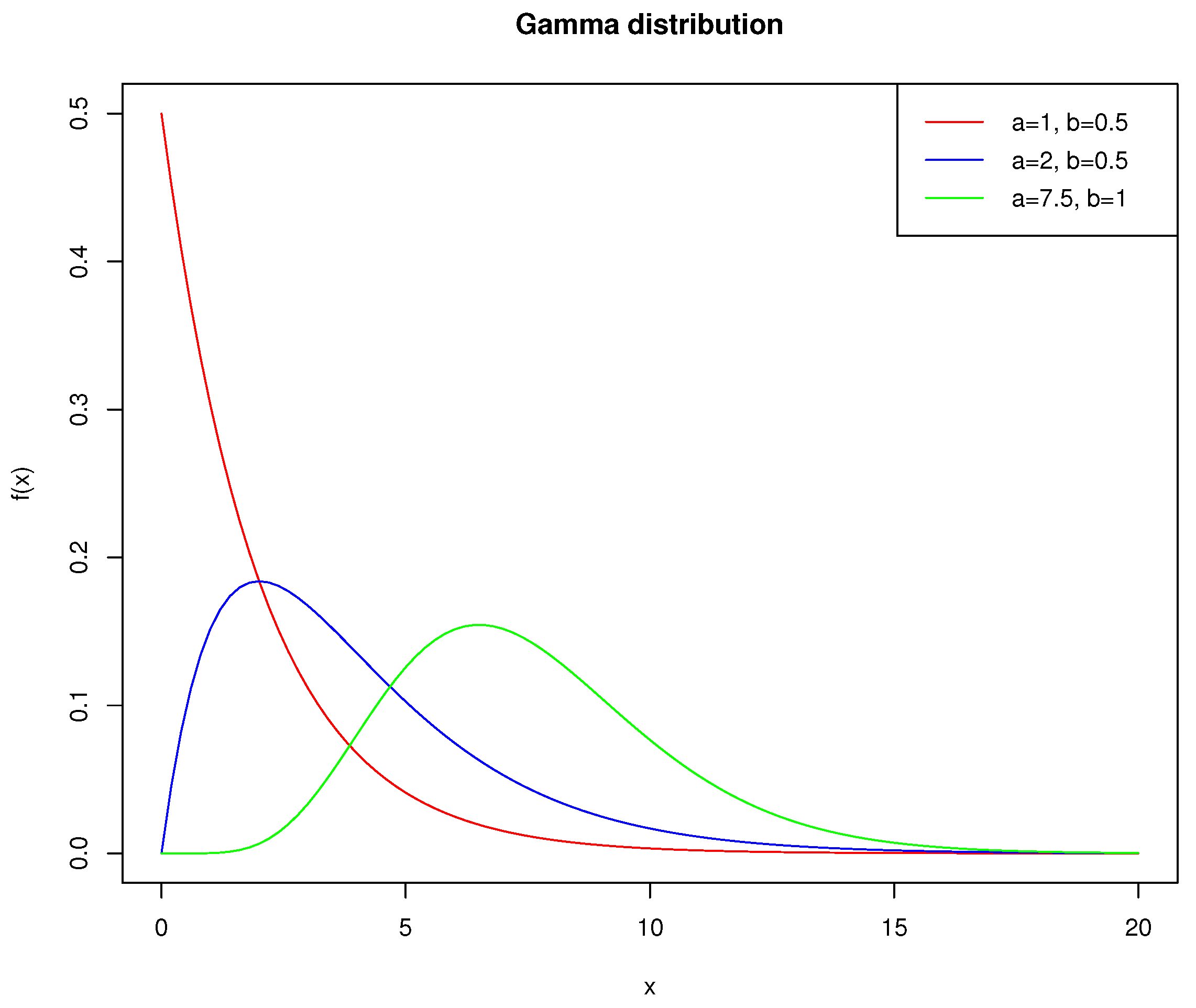
The proof of Theorem 3 is provided in Appendix A. Note that Theorem 3 is established not only for the gamma distribution but also for all continuous population distribution. Next, moments and estimates in (12) are calculated from MSE-RPs, NT-RPs, and MC-RPs of different $Ga(a,b)$. Three typical shapes of gamma distributions ($Ga(1,0.5)$—monotone decreasing; $Ga(2,0.5)$—right skewed and $Ga(7.5,1)$—bell-shaped; their pdfs are plotted in Figure 1). These are chosen and the representative points are set to three sizes ($k=5,20,100$). The first part of Table 1, Table 2 and Table 3 summarizes the results in different scenarios. The last line of each table presents the moments and parameters of $Ga(a,b)$. It is clear that if k is fixed, the moments and estimates of MSE-RPs are closer to the true values than other representative points. Moreover, we can observe that the means of MSE-RPs are almost equal to the means of $Ga(a,b)$ in all scenarios; when k becomes large, the moments and estimates of MSE-RPs converge to the true values much faster than other representative points. These results are consistent with the description in Theorem 3.

Figure 1. Probability density function for $Ga(1,0.5)$, $Ga(2,0.5)$ and $Ga(7.5,1)$.

Table 1. Summary of results from RPs of $Ga(1,0.5)$ in parameter estimation.

	k	$\mathit{\mu }$	${\mathit{\sigma }}^2$	$\mathbf{Skewness}$	$\mathbf{Kurtosis}$	${\widehat{\mathit{a}}}_{{\mathit{m}}_2}$	${\widehat{\mathit{b}}}_{{\mathit{m}}_2}$	${\overline{\mathbf{PD}}}_{{\widehat{\mathit{a}}}_{{\mathit{m}}_2}}$	${\overline{\mathbf{PD}}}_{{\widehat{\mathit{b}}}_{{\mathit{m}}_2}}$	${\overline{\mathbf{PD}}}_{{\widehat{\mathit{a}}}_{\mathit{mle}}}$	${\overline{\mathbf{PD}}}_{{\widehat{\mathit{b}}}_{\mathit{mle}}}$
	5	2.001	3.708	1.850	3.971	1.080	0.540	0.086	0.088	0.380	0.381
MSE-RPs	20	2.001	3.978	1.989	5.767	1.007	0.503	0.050	0.056	0.088	0.089
	100	2.001	3.998	2.003	5.996	1.002	0.501	0.050	0.056	0.036	0.043
	5	1.866	2.419	0.775	−0.752	1.440	0.772	0.441	0.545	0.244	0.334
NT-RPs	20	1.967	3.419	1.394	1.470	1.132	0.576	0.134	0.153	0.060	0.078
	100	1.995	3.839	1.759	3.662	1.036	0.520	0.054	0.059	0.034	0.043
	5	2.069	3.516	0.576	−0.839	2.720	1.586	1.818	2.312	1.569	1.939
MC-RPs 1	20	1.945	3.629	1.329	1.571	1.269	0.684	0.348	0.401	0.244	0.327
	100	1.991	3.987	1.751	3.797	1.051	0.536	0.168	0.181	0.108	0.127
$Ga(1,0.5)$		2	4	2	6	1	0.5	-	-	-	-

Table 2. Summary of results from RPs of $Ga(2,0.5)$ in parameter estimation.

	k	$\mathit{\mu }$	${\mathit{\sigma }}^2$	$\mathbf{Skewness}$	$\mathbf{Kurtosis}$	${\widehat{\mathit{a}}}_{{\mathit{m}}_2}$	${\widehat{\mathit{b}}}_{{\mathit{m}}_2}$	${\overline{\mathbf{PD}}}_{{\widehat{\mathit{a}}}_{{\mathit{m}}_2}}$	${\overline{\mathbf{PD}}}_{{\widehat{\mathit{b}}}_{{\mathit{m}}_2}}$	${\overline{\mathbf{PD}}}_{{\widehat{\mathit{a}}}_{\mathit{mle}}}$	${\overline{\mathbf{PD}}}_{{\widehat{\mathit{b}}}_{\mathit{mle}}}$
	5	3.999	7.396	1.304	1.685	2.163	0.541	0.085	0.086	0.222	0.223
MSE-RPs	20	3.999	7.954	1.403	2.842	2.011	0.503	0.044	0.048	0.042	0.046
	100	3.999	7.997	1.412	2.976	2.001	0.500	0.044	0.047	0.033	0.037
	5	3.855	5.449	0.552	−0.934	2.727	0.707	0.365	0.416	0.269	0.317
NT-RPs	20	3.963	7.149	1.010	0.532	2.196	0.554	0.101	0.112	0.061	0.071
	100	3.993	7.780	1.266	1.825	2.049	0.513	0.044	0.048	0.034	0.038
	5	4.089	6.912	0.416	−0.904	5.261	1.382	1.769	1.925	1.672	1.800
MC-RPs	20	3.917	7.269	0.969	0.755	2.425	0.633	0.310	0.339	0.260	0.304
	100	3.981	7.982	1.266	1.930	2.074	0.525	0.146	0.153	0.112	0.120
$Ga(2,0.5)$		4	8	1.414	3	2	0.5	-	-	-	-

Table 3. Summary of results from RPs of $Ga(7.5,1)$ in parameter estimation.

	k	$\mathit{\mu }$	${\mathit{\sigma }}^2$	$\mathbf{Skewness}$	$\mathbf{Kurtosis}$	${\widehat{\mathit{a}}}_{{\mathit{m}}_2}$	${\widehat{\mathit{b}}}_{{\mathit{m}}_2}$	${\overline{\mathbf{PD}}}_{{\widehat{\mathit{a}}}_{{\mathit{m}}_2}}$	${\overline{\mathbf{PD}}}_{{\widehat{\mathit{b}}}_{{\mathit{m}}_2}}$	${\overline{\mathbf{PD}}}_{{\widehat{\mathit{a}}}_{\mathit{mle}}}$	${\overline{\mathbf{PD}}}_{{\widehat{\mathit{b}}}_{\mathit{mle}}}$
	5	7.499	6.911	0.672	0.024	8.139	1.085	0.088	0.088	0.121	0.121
MSE-RPs	20	7.499	7.455	0.724	0.711	7.545	1.006	0.038	0.039	0.036	0.037
	100	7.499	7.498	0.730	0.795	7.502	1.000	0.038	0.040	0.035	0.036
	5	7.424	5.575	0.284	−1.067	9.885	1.332	0.319	0.333	0.296	0.309
NT-RPs	20	7.480	6.946	0.530	−0.213	8.056	1.077	0.076	0.079	0.067	0.070
	100	7.496	7.374	0.662	0.381	7.620	1.017	0.038	0.039	0.036	0.037
	5	7.575	6.394	0.225	−0.950	19.282	2.561	1.480	1.431	1.480	1.422
MC-RPs	20	7.416	6.901	0.494	0.076	8.754	1.187	0.286	0.296	0.277	0.290
	100	7.478	7.490	0.670	0.443	7.714	1.034	0.127	0.127	0.116	0.116
$Ga(7.5,1)$		7.5	7.5	0.730	0.8	7.5	1	-	-	-	-

Next, the comparison focuses on the estimating performance of samples from representative points. We take samples from different shapes of gamma distributions ($Ga(1,0.5)$, $Ga(2,0.5)$ and $Ga(7.5,1)$), as well as their representative points with different sizes ($k=5,20,100$). Setting sample size $N=1000$ and repeat sampling $M=10,000$ times for each scenario, the method of moment estimates (${\widehat{a}}_{m_2}$ and ${\widehat{b}}_{m_2}$) and maximum likelihood estimates (${\widehat{a}}_{mle}$ and ${\widehat{b}}_{mle}$) are calculated. Define

$$\begin{array}{c}\hfill {\overline{\mathrm{PD}}}_{\widehat{a}}=\sum _{i=1}^M\frac{|{\widehat{a}}_i-a|}{a}/Mand{\overline{\mathrm{PD}}}_{\widehat{b}}=\sum _{i=1}^M\frac{|{\widehat{b}}_i-b|}{b}/M\end{array}$$

as the average proportional deviation between estimations and parameters. The second part of Table 1, Table 2 and Table 3 show that MSE-RPs samples have the smallest average proportional deviation in most of the selected scenarios. Table A1 and Table A2 in Appendix C give medians and 95% empirical confidence intervals of ${\widehat{a}}_{m_2}$, ${\widehat{b}}_{m_2}$, ${\widehat{a}}_{mle}$ and ${\widehat{b}}_{mle}$. In this simulation study, we observe that the point estimates of a and b from MSE-RPs samples generally have good estimation accuracy with both the moment and maximum likelihood methods. Meanwhile, when k is large, the estimation performances of MSE-RPs samples are similar to those samples from the corresponding $Ga(a,b)$. It is also worth mentioning that when $k=5$, the proportional deviation ${\overline{\mathrm{PD}}}_{{\widehat{a}}_{m_2}}$ and ${\overline{\mathrm{PD}}}_{{\widehat{b}}_{m_2}}$ are much smaller than ${\overline{\mathrm{PD}}}_{{\widehat{a}}_{mle}}$ and ${\overline{\mathrm{PD}}}_{{\widehat{b}}_{mle}}$. That is, when the size of gamma MSE-RPs is small, it is better to estimate parameters using the method of moments.

5. Generating MSE-RPs from Harrel–Davis Standardized Samples

This section discusses how to generate MSE-RPs from a gamma-distributed sample. A commonly used approach has two steps as follows:

• Calculate the maximum likelihood estimates (MLEs) for a and b, namely $\widehat{a}$ and $\widehat{b}$, based on the sample dataset;
• Generate MSE-RPs from the gamma distribution with the estimated parameters, i.e., $Ga(\widehat{a},\widehat{b})$.

As we know, the representativeness of MSE-RPs depends on the estimate of gamma parameters. More accurate estimates will produce better representativeness. However, if a random sample does not represent the population well, the estimates may show large deviations from the true parameters. Hence, the MSE-RPs that are generated are not good representatives of the population distribution. This usually occurs when the sample size is small or medium. Next, we introduce a new Harrel–Davis (HD) standardization technique that can reduce the effect of randomness from samples. This technique transfers a random sample to a set of HD quantile estimators and then treats these estimators as a new “sample”. Recall that a set of quantiles with equal probability is a set of NT-RPs for population; a similar idea is utilized for sample standardization.

Definition 1

(HD standardized sample). Let $x=\{x_1,x_2,\cdots ,x_n\}$ be a set of sample data from a gamma distribution; set $x^{\prime }=\{Q_{p_1},Q_{p_2},\cdots ,Q_{p_n}\}$, which is called the HD standardized sample of x, where $Q_{p_i}$ is the $p_i$th HD quantile estimator defined in (6), $p_i=\frac{2i-1}{2n}$ and $P\left(Q_{p_i}\right)=1/n$ ($i=1,2,\cdots ,n$).

Note here that $x^{\prime }$ is not a random sample because $Q_{p_1},Q_{p_2},\cdots ,Q_{p_n}$ are not independent. However, since quantile estimators are equiprobable ($P\left(Q_{p_i}\right)=1/n$), set $x^{\prime }$ is treated as an arbitrarily selected sample, which can be used to calculate MLEs for a and b. A new approach to generate MSE-RPs is proposed as follows:

• Obtain the HD standardized sample;
• Calculate the MLEs for a and b, namely $\widehat{a}$ and $\widehat{b}$, based on the HD standardized sample;
• Generate MSE-RPs from $Ga(\widehat{a},\widehat{b})$.

Next, a simulation study is provided to show the good performance of HD standard samples in parameter estimation. Consider three gamma distributions ($Ga(1,0.5)$, $Ga(2,0.5)$ and $Ga(7.5,1)$) and three different sample sizes ($n=50,200,500$), in each scenario, a number of $N=10,000$ random samples are generated and their HD standardized samples are obtained. The MLEs are calculated for each sample/standardized sample and summarized in Table 4. This shows that the means of estimates from HD standardized samples are closer to the true value in most scenarios. Moreover, the estimates from HD standardized samples appear to have smaller standard deviations than those from random samples. We conclude that HD standardized samples outperform random samples in terms of estimation accuracy and stability based on these results. Therefore, it is recommended to use the new three-step approach to generate MSE-RPs. Here, a comparison study between the MSE-RPs generated by random samples and HD-samples is provided. The estimates ($\widehat{a}$ and $\widehat{b}$) in Table 4 are used to generate gamma MSE-RPs. Table 5 summarizes the results when $n=200$ with the size of MSE-RPs $k=20$. It shows that the moments of gamma MSE-RPs from HD-samples are close to the moments of the origin $Ga(a,b)$. Meanwhile, the method of moment estimates in (12) are obtained. The estimates from HD samples have a better accuracy than those from random samples. This conclusion is generally valid when $n=50and500$.

Table 4. Mean (Standard deviation) of MLEs from samples and HD standardized samples.

		$\mathit{Ga}(1,0.5)$		$\mathit{Ga}(2,0.5)$		$\mathit{Ga}(7.5,1)$
$\mathit{n}$		Sample	HD-Sample	Sample	HD-Sample	Sample	HD-Sample
50	$\widehat{a}$	1.060(0.195)	1.075(0.192)	2.115(0.415)	2.104(0.405)	7.964(1.645)	7.794(1.604)
	$\widehat{b}$	0.540(0.127)	0.535(0.126)	0.534(0.118)	0.524(0.116)	1.064(0.227)	1.038(0.221)
200	$\widehat{a}$	1.021(0.090)	1.020(0.090)	2.029(0.192)	2.012(0.189)	7.616(0.759)	7.502(0.746)
	$\widehat{b}$	0.512(0.058)	0.507(0.058)	0.508(0.054)	0.502(0.054)	1.016(0.104)	0.999(0.103)
500	$\widehat{a}$	1.012(0.056)	1.010(0.056)	2.010(0.120)	2.000(0.119)	7.543(0.472)	7.477(0.468)
	$\widehat{b}$	0.507(0.036)	0.504(0.036)	0.503(0.034)	0.499(0.033)	1.006(0.065)	0.997(0.064)

Table 5. Summary of results for MSE-RPs from the esitmated gamma distributions.

$\mathit{n}=200$	$\mathit{k}=20$	$\mathit{\mu }$	${\mathit{\sigma }}^2$	Skewness	Kurtosis	${\widehat{\mathit{a}}}_{{\mathit{m}}_2}$	${\widehat{\mathit{b}}}_{{\mathit{m}}_2}$
	sample	1.995	3.873	1.966	5.641	1.028	0.515
$Ga(1,0.5)$	HD-sample	2.013	3.946	1.967	5.647	1.027	0.510
	origin	2	4	2	6	1	0.5
	sample	3.994	7.818	1.393	2.801	2.041	0.511
$Ga(2,0.5)$	HD-sample	4.008	7.938	1.399	2.825	2.023	0.505
	origin	4	8	1.414	3	2	0.5
	sample	7.496	7.334	0.719	0.699	7.662	1.022
$Ga(7.5,1)$	HD-sample	7.509	7.472	0.724	0.711	7.547	1.005
	origin	7.5	7.5	0.730	0.8	7.5	1

It is noteworthy that the HD standardization technique can also be applied in resampling. Consider another simulation study with the same settings as Table 4. We resample from each sample/standardized sample using $n_r=n$ and calculate the MLEs. The means and standard deviations of the resampled MLEs are summarized in Table 6. This shows that estimates from standardized samples generally have a better accuracy and smaller standard deviations when resampling.

Table 6. Mean (Standard deviation) of resampled MLEs from samples and HD standardized samples.

		$\mathit{Ga}(1,0.5)$		$\mathit{Ga}(2,0.5)$		$\mathit{Ga}(7.5,1)$
n(${\mathbf{n}}_{\mathbf{r}}$)		Sample	HD-Sample	Sample	HD-Sample	Sample	HD-Sample
50	$\widehat{a}$	1.114(0.295)	1.127(0.283)	2.234(0.630)	2.216(0.594)	8.446(2.504)	8.245(2.340)
	$\widehat{b}$	0.577(0.196)	0.572(0.185)	0.569(0.181)	0.558(0.170)	1.131(0.347)	1.101(0.323)
200	$\widehat{a}$	1.034(0.131)	1.030(0.127)	2.059(0.279)	2.034(0.269)	7.741(1.102)	7.594(1.061)
	$\widehat{b}$	0.522(0.085)	0.515(0.082)	0.518(0.079)	0.509(0.076)	1.034(0.151)	1.013(0.146)
500	$\widehat{a}$	1.017(0.079)	1.016(0.079)	2.021(0.167)	2.012(0.168)	7.584(0.660)	7.527(0.662)
	$\widehat{b}$	0.510(0.051)	0.508(0.051)	0.506(0.047)	0.503(0.047)	1.012(0.091)	1.004(0.091)

6. Real Data Illustration

In this section, we consider a real-world dataset and illustrate the HD standardized technique proposed in the previous section. In this clinical study, 97 Swiss females ($n=97$) aged 70–74 inclusive at the time of diagnosis of dementia (a form of mental disorder) were studied for survival times (in years) by Elandt–Johnson and Johnson [23]. These data were analyzed by Ozonur and Paul [24] using the likelihood ratio test and score test with p-values 0.233 and 0.140, which are greater than 0.05. Both tests suggest that the two-parameter gamma distribution adequately fits the dementia data.

Point estimates (MLE) and the bootstrap interval estimates [25] based on the origin sample data and the corresponding HD sample are calculated. The approximate ($1-\alpha$) bootstrap percentile interval is defined as

$$\left[{\widehat{\theta }}_{\mathrm{lower}},{\widehat{\theta }}_{\mathrm{upper}}\right]=\left[{\widehat{\theta }}_M^{*\left(\frac{\alpha }{2}\right)},{\widehat{\theta }}_M^{*\left(1-\frac{\alpha }{2}\right)}\right].$$

In practice, we resample the original data $M=1000$ times to obtain 1000 replications of the parameter estimate ${\widehat{\theta }}^{*}$ (i.e., $\widehat{a}$ and $\widehat{b}$ for the gamma distribution) with $\alpha =0.05$. These estimates are sorted and the 25th value is used as the lower bound; the 975th value is the upper bound. The MLEs based on the HD standardized sample are ${\widehat{a}}_{HD}=1.4602$ and ${\widehat{b}}_{HD}=0.2886$ with confidence intervals $(1.3846,1.8073)$ and $(0.2637,0.3839)$. The lengths of confidence intervals are shorter than those based on the origin sample data, where ${\widehat{a}}_{origin}=1.4602$ and ${\widehat{b}}_{origin}=0.2886$ with confidence intervals $(1.3777,1.8632)$ and $(0.2659,0.3914)$.

7. Concluding Remarks

In the first part of this paper, the existence and uniqueness of gamma MSE-RPs are proved using two different approaches. An effective algorithm is recommended for the generation of gamma MSE-RPs. The second part of this paper compares gamma MSE-RPs with other representative points in terms of parameter estimation and simulation. This shows that the moments and estimates based on gamma MSE-RPs are the closest to the true values in different scenarios. In addition, samples from gamma MSE-RPs show a good general estimation accuracy. The last part of this paper introduces the new HD standardization technique. When a gamma-distributed sample is at hand, we recommend first transferring it to the HD standardized sample and then using it to estimate gamma parameters or generate MSE-RPs.

In future work, we would like to study whether the MSE-RPs of other distributions can also perform well in parameter estimation. It would also be interesting to explain how HD standardization technique reduces the randomness from samples through a theoretical demonstration.