Abstract
Our proposed method for exploring the causal discovery of stochastic dynamic systems is designed to overcome the limitations of existing methods in detecting hidden and common drivers. The method is based on a simple principle and is presented in a nonparametric structural vector autoregressive modeling framework.
MSC:
62D20; 60J10; 62M99; 92F05
1. Introduction
Causality has long been a puzzling question in both general and natural philosophy. The concept of necessary causation was first formulated by the school of Hippocrates, more than hundred years before Aristotle [1]. Understanding causal relationships between systems is a crucial aspect of modern science. This can be achieved by analysing the events or time series generated by systems, either through intervention or purely observational methods.
The interventional, experiment-based approach was formalized in the axiomatic framework of Pearl [2], while for the noninterventional scenario, the predictive causality principle was formulated by Wiener [3], and its practical realization was developed by Granger [4]. The Granger method is widely applied, although it has theoretic and practical limitations. The method is very popular, but it is not able to detect a hidden common cause (called confounders or cointegration by the Granger school causality).
All variations and generalizations of the predictive causality principle, including those mentioned in [5], suffer from the same limitations as the original method. In the last two decades, several new methods have been developed to address these limitations (for a concise review, see Balasis [6] or Runge [7]). One of the most prominent is the convergent cross-mapping method developed by Sugihara [8], which relies on Takens’ embedding theorem [9]. This theorem allows the reconstruction of the state space of system under investigation from an observed time series under suitable conditions. Sugihara’s method is based on this reconstruction, which examines the behavior of the driver and the driven systems and the cross-space mapping between them. All methods based on Takens’ theorem assume that the investigated systems are deterministic dynamic systems. Stark [10,11] has shown that Takens’ result can be generalized to stochastic systems to some extent, but this generalization has important theoretical limitations.
Exploring causal relationships between stochastic dynamic systems, based solely on observed time series of their states, is a challenging problem. In this paper, a method is presented that is based on a simple observation: a process generated by a stochastic dynamical system is a Markov chain if and only if all external influences are independent and identically distributed (i.i.d.). Therefore, the key tool of our proposed causal discovery scheme is to test whether the process generates a Markov chain rather than the “classical” causal Markov property or d-separation (as described in [2,12], and the recent work [13]). Our method is nonparametric, it requires no intervention, and it has a reasonably small number of assumptions.
In this paper, in relation to dynamical systems, we use the terms drive, cause, influence, injecting information as synonyms.
The paper is organized as follows: In Section 2.1, basic definitions and assumptions are given, followed by Section 3 with the key observation on the recursive definition of Markov chains and its direct consequences. Section 4 provides a detailed description of how the analysis of Markov property and information exchange allows different casual scenarios to be detected. Section 5 describes the statistical analysis and illustrates how the method can be applied to two different processes. The paper concludes with a further recall of related works, a discussion of capabilities and limitations, and finally some concluding remarks.
2. Preliminaries
In a recent work [14], a new method was developed for deterministic dynamic systems, which can detect the presence of a hidden common cause without intervention. There it is assumed that the time series are in their stationary state, and the samples are taken from this time-indexed stationary distribution. The investigation boils down to the observation that
and there is a common cause if there is a strict inequality on both sides. (Here, H stands for the Shannon entropy and both the individual and the joint distributions of X, Y are stationary). The case holds if X causes Y and trivially they are independent if if . Unfortunately, such argument fails for stochastic dynamic systems, as well as if the observation is noisy, as the following example shows.
Example 1.
Let X and Y be two deterministic dynamical systems and let X be observed with some noise. If the noisy process is denoted by , it is easy to see that even if X drives (causes) Y,
It is to be noted that neither the entropy of the stationary distribution of the variables nor the dimension of the state space can accurately reflect causation, resulting in a false detection of common cause rather than direct causation.
One of the main motivations for developing the method presented in this paper is the ability to detect causal relations between stochastic dynamic systems (and noisy observations of deterministic systems as well). It is important to note that causal discovery in general has theoretical limitations, as Markov equivalent directed acyclic graphs (DAGs) cannot be distinguished without intervention, and these limitations are even greater when a proportion of the variables are unobserved. Our method aims to address these limitations by detecting all types of possible causal connections between correlated time series, including hidden common causes. This makes it a versatile tool for identifying complex causal relationships in both synthetic and real-world data.
2.1. Basic Definitions
We will denote the fact that the system A or the sequence which we observe is a Markov chain by (or .
First, we provide the framework of our investigation. Our aim is to find the causal relationship between two stochastic dynamic systems, X and Y, from which we observe the time series . The time-delay embedding of a series (scalar or vector) will be denoted by . Here, m is the embedding dimension and is the time delay. Throughout the sequel, we will use the convention of lower case to denote the original series, and upper case to denote the embedded series by the time index. To abuse the notation somewhat, capital letters without a time index will refer to the system (X) from which the series () are observed.
Let us use the following notations: is a latent process (a collection of latent processes) that drives X but not Y, and similarly, denotes a process that drives Y but not . Let denote a latent process (a collection of latent processes) that drives both X and . Assume that , and Z inject into X or Y non i.i.d. information. If there is an i.i.d. sequence that drives both X and Y, let it be denoted by .
In this paper, we consider the simple situation where the time lag between the investigated systems is unity, and the same is true for the common driver. As a consequence, the lag difference is zero. This assumption simplifies the picture significantly, and even provides the exceptional possibility to pinpoint whether a common or a direct driver is present. Unfortunately, in general, that is not the case. More general (and cumbersome) scenarios are a matter of future works.
The processes involved can be discrete or continuous in both space and time, but actual observations can only result in being discrete time series. A detailed description of the observed processes can be given using the conventions and assumptions listed above:
Assumption 1.
We assume that there is a set of systems ,
,
,
,
and a set of external source of noises
such that the process
has a joint distribution.
The series are unobserved, hidden series that are injecting non i.i.d. into or .
It can observed that (or ) falls within the framework of SEM (Structural Equation Modeling) as defined by Perl [2], or in other terms, it can be described as a linear or nonlinear first-order Structural Vector Autoregressive model (c.f. [13] ):
We use the same restriction as in [13] that (6) must be recursive in the variables that ensure that there is no directed functional cycle.
In fact, in our discovery scheme, we may allow instantaneous causation between all variables. For brevity, this is not reflected in (6), and is not discussed in this paper. We also note that a system like (6) with contemporaneous interaction, but without a directed cycle, can be rewritten into the form of (6), thanks to the acyclic recursivity. Multiple lags are also not discussed, those can be handled by more complex CIT-s, but without new theoretical arguments.
Assumption 2.
The external noise is modelled by the unobserved which is i.i.d. and affects each system separately, with independent components. Furthermore, is independent from .
Assumption 3.
The joint process is stationary.
Assumption 4.
The investigated process is exact (c.f. [15] Definition 4.3.2).
Assumption 5.
The causal structure of the time series is time invariant and non random.
3. Markov Property
Lemma 1.
Let us assume that the time series has the following evolution equation:
where (). Then, is a first-order Markov chain if and only if is an i.i.d. sequence (see [16] Exercise 1.1.3).
One can see that described in (6) is a Markov chain, but we will not use this fact directly. Let us mention that recursive frameworks such as (6) are used in several papers—however, their Markov property is not observed and utilized.
We are going to study the causal relation between X and Y, using Lemma 1. Imagine the particular case where X drives Y, but only an i.i.d. sequence is injected into Y via the evolution equation:
Such a situation can be interpreted as X drives Y, but it also can be argued that the i.i.d. sequence is a common driver for both X and Y. In fact, there is no way to distinguish between the two scenarios, if we can not do intervention. Following Occam’s razor principle, it can be assumed that X drives Y, instead of assuming that there is a third common driver.
Definition 1.
We will say that X drives Y if
where is an i.i.d. sequence and independent of , but there is no function g s.t.
where is an i.i.d. sequence, independent of .
The absence of g described in (9) means that, in (8), X has true influence on Y, and its presence in (8) is not formal.
Lemma 1 has some immediate consequences.
Corollary 1.
Let us assume that X drives Y and the injection from X to Y via f is not i.i.d.; then, is not a first-order Markov chain.
Before starting the systematic analysis, let us present a simple observation that helps to identify the direction of a causal relation.
Lemma 2.
Proof.
By the definition of ,
and similarly
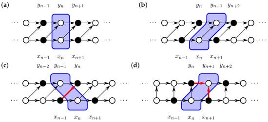
For and , the above simple reformulation and Lemma 1 ensures the Markov property, as is demonstrated in Figure 1a,b, while for , the propagation of information from past to future (indicated by the red arrow in Figure 1c) from X to Y, is regardless of the condition. Observe that, if the information from injected into is only an i.i.d. sequence, then there is no driving since it contradicts the condition that there is no g satisfying (9).
Figure 1.
Markov property and unidirectional forcing. Conditional independence tests to test the Markov property under various lag configurations are illustrated. The condition is indicated by the shaded area, while the observations used in the dependence test are represented by filled circles. (a) When no lag is assumed, and (correctly) appear independent given . (b) Assuming (the true) 1-step lag for effect propagation from x to y, then the lag-corrected joint system (correctly) appears as Markov. (c) Assuming a 1-step lag in the wrong direction, the joint is not Markov due to the information flow indicated by the thick red arrow; (d) the case of contemporaneous action. This is not studied in depth in this paper. However, this example serves as a demonstration for possible errors if the lag is incorrectly identified. Assuming a 1-step lag instead of an instant action, the joint does not appear to be Markov due to the collider node indicated by the thick red arrows. See Section 6.2.1 for an application. Note: the same situation occurs for the 1-step effect propagation lag, if one falsely assumes a 2-step lag (not depicted here).
□
It is possible that X (or Y) injects an i.i.d. sequence into the other. In short, we refer to that situation by i.i.(Independent Injection) that will be denoted by and, in some places, we will use to emphasize the opposite, that the driving takes place via a non i.i.d. sequence.
In the following, the cases of causality are listed that can be detected by verifying the Markov property of the processes , and measuring the level of dependence between their different combinations.
4. Markov Chains
While in [17] (2.8)(1) many observed processes are handled, we restrict our attention to two observed processes for simplicity of presentation, but note that all arguments and methods can be extended to multiple processes at the price of executing more independence tests and separation of cases. In the following, we will use the abbreviation standing for any dependence measure that is zero if and only if A and B are independent given C. (As an example, I can be conditional mutual information, and for simplicity, we will use this terminology, but, in practice, it will be replaced with a more-statistically well-behaved dependence measure.)
We will need to test (measure) the dependence of several combinations of variables:
Here, for (similar notation will be used for other variables as well).
The above conditional mutual information is used as indicators for Markov property of . The large number of cases under investigation can not be incorporated into a readable single equation. We split the set of cases with respect to very basic properties. First, we assume that , i.e., J forms a Markov chain, then we drop this and introduce subcases under the condition . We will proceed gradually from simple conditions to more complex ones, and finally reach a full list of all possible cases.
Let we start with the assumption that is a first-order Markov chain (denoted by ) which greatly simplifies the analysis and helps to demonstrate the simple but crucial arguments. The Markov property of J holds iff .
Case 1:
Clearly, must not be present; otherwise, the Markov property of J would be violated. One can immediately observe that iff is not present. For a concise discussion, let , (or and , respectively). It is easy to observe that
Since J is Markov (as assumed in Case 1), and if and , then Figure 1a) depicts the situation well: the next state of the joint processes is simply obtained from the current state of the joint processes—however, if Y is not Markov, even though X and Y together are Markov, then it means that there must be some information in X that is needed to find the next state of Y. This implies, however, that the dependence between X and Y is non-zero , and that there is driving from X to Y.
Here, and throughout the sequel, will denote that the injected information is i.i.d., denotes that it is not i.i.d., and → denotes that there is a driving but its nature cannot be further specified. Let us summarize the above implications: where denotes the situation if the given chain is a first-order Markov chain, and by if not. The presence of a process or a causal relation will be denoted by ∃ and its absence is denoted by n (non). If a test is indifferent, the cell will contain a − sign. The column headed by indicates if i.i.d. input from one observed series to another is forbidden (f) or allowed (a). The mark * indicates the impossible cases.
Here, and in the following equations, the cases are direct products of the cases in the two curly brackets. The left and right part of the curly brackets are separated by implication arrows. The left parts contain the list of cases and the possible outcome of independence tests, and the right parts contain the consequences.
Note that (10) contains all possible cases under the condition . The cases are also mutually exclusive, which means that the implications ⟹ can be replaced by the ⇔, if and only if relations. In the following, we consider the case and again all possible sub-cases. Thus, our analysis will contain all mutually exclusive cases and all the implications are in fact the iff only iff type.
In (10), (11) and in (12), the investigated properties are to the left from the arrows, and the conclusion and causal relations are to the right of them. The product of the curly brackets indicates the direct product of the possible cases in them. Under the , the symbol means that the process in Markov, and the opposite. Under , f indicates that i.i.d. transfer between A and B is forbidden, and a that it is allowed. On the right, n indicates nonexistence, that the injected information is i.i.d., while that it is not. * indicates that the combination on the left is impossible.
Case 2:
It is immediately clear that, for ⇔, there is a common driver (Z or ). It is also clear that, if , it is impossible that A and . If , at least one of Z, and is present.
Subcase 2.1: and
If , it is sure that there is no or Z.
Let us observe that, from and
it follows that there should be to ensure in the case of that and if to ensure . These observations are expanded to scenarios in (11).
Subcase 2.2:
We know that and or Z should be present.
In the third row of (12), we have to see that not all the cases can be distinguished. This is the first case of this kind. The condition holds only if at least one of the “external” drivers or Z is present, but without intervention, we cannot tell which one. That situation is indicated by . From Row 4 onward, the situation (marked by ) is even less determined. The observation can be the consequence of the presence of or Z. Of course, if Z is present, we cannot detect .
If we assume that only is present (Z is not), then different hidden scenarios hold for each row.
Row 4. and the assumption implies the presence of and ,
Row 5. and the assumption implies the presence of , but may or may not exist,
Row 6. and the assumption implies the presence of or .
On the contrary, conditions are satisfied in the presence of Z, and no information can be gained on the existence of and .
As we mentioned, the case where there are multiple lags or lag differences can be treated similarly with proper but more cumbersome conditioning which we do not elaborate on here.
Practical algorithmic and statistic discovery of causal relations can more or less follow the logic of the above analysis, starting with simpler tests and cases, and gradually incorporate more and more, as the gained information shows their necessity.
5. Inference
5.1. Preconditions and Preprocessing
As an initial step, we have to test if the investigated series are correlated (in nonlinear sense, their mutual information is not zero). Otherwise, there is certainly no casual relation between the systems under investigation.
Next, we should find the time lag between the series, finding the lag that produces the maximal cross-correlation (again in linear or nonlinear sense). Using partial correlation is preferable, as it removes some level of spurious correlation.
As stated, we need time series to be results of observing stationary processes. This can be achieved by appropriate prepossessing of the series, for example by detrending the series, removing periodicity, or other methods not elaborated here.
Next, we should transform the series into order one processes by using time delay embedding. There are no general recipes for this step; it depends very much on the actual process. It is generally accepted that a higher-order process can be transformed into an order one process by a sufficiently large embedding dimension. There is no general rule for the choice of the the embedding dimension. If the chosen dimension is too low, we still have a higher order process, if we use a high embedding dimension, we run into the usual problems of lack of enough sample elements or extremely large run-time. As a rule of thumb, we should use the largest possible embedding dimension, where the autocorrelation is very short and we still have enough samples for the analysis.
It is also possible that the observations are noisy, and some noise reduction is needed. Again, there is no consensus in this respect. It is far from trivial which part of the stochastic behavior is the effect of mere observational noise or an inherent part of the process. Therefore, removal requires particular information (possibly, domain expertise) about the sources of the series and the possible noise.
5.2. Testing
The conditional independence test (CIT) has recently become a focus of research, motivated by the many applications of machine learning and artificial intelligence. It is well known that it is a challenging task [13,18,19,20]. The importance of dependence measures is also reflected in a large number of proposed measures and the still ongoing research to find new testable and efficient measures (cf. the papers [21,22] and their bibliography). The present paper does not intend to develop a new CIT or dependence measure, but rather to apply a suitable one which supports our causal discovery scheme.
Clearly, a conditional independence test is needed to test the Markov property. Consequently, the various tests listed in Section 4 can boil down to CITs. The general schema is , where D is a dependence measure, which indicates the independence of given C by taking value zero. In general, a dependence measure should satisfy some straightforward assumptions (cf. Rényi [23]). Here, the key for us is that
if and only if the random variables A and B are independent and D has a known null distribution, and consequently, it is testable. We need several variations of the CIT. Let us give the simplest example. When we test if is a Markov chain, we investigate and .
There are several technical difficulties in performing a CIT. Testing independence runs immediately into the problem of the curse of dimensionality when the condition must cover a longer part of the process history. If we aggregate the states in order to decrease the number of samples required, we have the same problem as in the continuous variable case, as described below. Imagine that we have a (finite) partition of the range of the variable C and an that contains more than one of the possible values. In this case, even if A and B are independent of all , they are not necessarily independent given , due to the fact that some information about the actual value can be present both in A and B. Runge suggests in [24] a surrogate method using local permutation to tackle this problem, which is used for the second example in Section 6.
Let us recall Assumption 5. As a consequence, there is no random information in the initial variable which is kept forever in the system. From Assumptions 3 and 4, we have that
as d tends to infinity. Unfortunately, this can not be tested given that there are invisible parts of the system M. Either we use a priori the Assumption 4 or investigate If is not converging to zero, we can not perform further causal discovery without collecting more information about our subject. If tends to zero, it makes it more acceptable to assume strong mixing, and (13) is satisfied.
Note that, for CIT, we use a member of the power divergence family, the modified log-likelihood method, instead of conditional mutual information.
5.3. Implementation Details
In addition to the difficulties mentioned in the preceding section, there are a number of problems that plague the practical implementation. Before adding a pseudo code for implementation, such important details have to be addressed. First, let us look at the outline of the general testing procedure:
- Do preprocessing (see Section 5.1);
- Find the most significant lag where the two time series are the most dependent (for example, simple or partial cross-correlation can be used for this);
- Make the time series stationary (remove trend, seasonality, …etc.);
- Find the memory of the processes (e.g., with partial auto-correlation);
- Apply time-delay embedding to convert a order Markov chain to a 1st order Markov chain;
- Based on the remaining rows, check which of the dependence measures need to be tested for significance (i.e., being greater than zero), and filter out additional rows;
- The remaining row represents the possible causal case that is in alignment with the data.
We would like to emphasize that the main contribution of this paper is meant to theorize how significance testing of the Markov property can help separate causal cases. The implementation and full-fledged analysis of a particular realization of the general procedure is beyond the scope of this paper. However, in order to demonstrate the validity of the theoretical foundations, we analyze a handful of datasets (see Section 6) with implementations specifically tailored for their corresponding dataset.
Among our test datasets (as in many real world cases), some are based on continuous Markov processes, making significance testing of conditional independence somewhat difficult. The technical difficulties we face are:
- How do we even test the Markov property? Assuming a discrete-valued time series, if we select a single point in time and consider it to be the “present” (according to the Markov property), then the previous data point from the present is the past, and the subsequent data point from the present is the future. We can loop through the time series and look for the same value that we currently have as present, and we can also collect the past and future values around those points in time. Thus, we practically found all possible conditional state transitions, given that one specific value of the condition. In order to test the Markov property, we need to do an independence test between these past and future values. In principle, a number of independence tests could be used; the choice is up to the researchers—in this particular implementation, we proceed with contingency-tables (having their own difficulties, see Items 3–4 below). Calculating a p-value is not trivial either (see Item 5 below), but even if we manage to do that, the Markov property is only proved locally because we analyzed a single value of the condition;
- To extend the testing procedure from a local property to a global one, we take all possible values of the condition and calculate a local p-value for each of them. The idea is that, strictly speaking, if the Markov property holds for all possible values of the condition, then we can say that the Markov property holds for the process in general. In this way, we run multiple hypothesis tests, leading to a multiple comparisons problem with dependent tests (since all the tests run on the same data)—in such cases, the harmonic mean of the p-values is a good proxy for the actual, global p-value (see [25]);
- We also need to handle continuous time series. Choosing an independence test for discrete variables requires some preparation before applying it to continuous data. First, if we select a specific point in time and consider it to be the present (i.e., we want to condition on it), then if we would like to collect all the related pasts and futures, it is impossible because we will not find the exact same value twice. To circumvent this issue, we find the k nearest neighbors (specifically, their indexes) for each “present’’ and consider them to be roughly equal (of course, k should be small, preferably vanishing compared to the sample size—for example, the square root of the sample size);
- We also need to discretize continuous time series. The most common way to discretize the data is to apply binning, but due to the time-delay embedding, we work with higher dimensional vectors for X and Y (and J, of course). If we binned along each dimensions, the amount of data would rapidly become insufficient for hypothesis testing, which would be especially problematic for smaller sample sizes. Instead of binning the embedded vectors along each dimension, we project the vectors onto a one-dimensional subspace (practically, combine a vector into a scalar with a linear transformation). Using random projections is one way to achieve this, which can be followed by the actual binning. However, using a single linear transformation for the whole time series may not work well; therefore, local random projections have to be repeated, i.e., different normal vectors have to be used and then the resulting p-values must be aggregated.
- In principle, it is up to the researcher to decide which independence test to use. As mentioned above, we have chosen contingency-tables in our examples. The problem with these is that our sample points are in general not independent; therefore, the analytical (or asymptotic) distribution of the test statistic is likely unavailable. To circumvent similar issues, bootstrapping-like techniques are commonly used to numerically approximate the cumulative distribution function of the test statistic. We apply the local permutation technique (proposed by Runge et al. [24]) to approximate the CDF of the test statistic under the null-hypothesis, which is then used to calculate the global p-value.
- Another technical issue is that filling in a contingency table based on a local neighborhood can easily lead to zeros appearing in the low probability cells of the table. For -like tests, this immediately leads to a p-value of 0, and even if a single local p-value is 0, then the global p-value obtained by taking their harmonic mean is badly affected. To avoid division by 0, we apply Yates’ correction to the contingency table to avoid strictly 0 local p-values.
The general procedure points out that a measure of dependence needs to be calculated and tested for significance under different inputs (and conditions) to filter out causal cases that are incompatible with the data. Note that, in the examples shown, this is equivalent to checking the Markov property of not just of X, Y, and J, but also of the direct product of X and Y given different offsets/lags. Therefore, we did not implement any measure of dependence—the causal cases are simply identified by testing the Markov property. We distilled these ideas into pseudo -ode: Algorithm 1 describes the overall procedure, while Algorithm 2 shows the hypothesis testing of the Markov property of a time series.
| Algorithm 1 Procedure for finding the p-value of Markov property for the time series separately, and their joint time series, given lags 0, 1, and −1. | |
| Require: | x: sample, the first time series (preprocessed) |
| Require: | y: sample, the second time series (preprocessed) |
| Require: | m: integer, memory; maximum of the largest significant lags of the two chains |
| Require: | r: number of times the local permutations should be repeated to bootstrap the |
| test statistic | |
| Require: | k: size of the local neighborhoods in which permutations are performed, shall be |
| less than used for the dependence testing; for details, refer to [24]. | |
| for do | |
| for r do | |
| end for | |
| end for | |
| Algorithm 2: The function responsible for testing Markovness of a time series (via conditional independence testing). | |
| Require: | : the time-series where the Markov property is to be tested |
| Require: | : the list of unique values upon which conditioning is to be carried out |
| (possible values of the “present”) | |
| for to do | |
| end for | |
| return | |
| * In our implementation, the independence test is the modified log-likelihood test. | |
6. Examples
The proposed method needs extensive testing on simulated and real-world data.
6.1. Simulated Data
Here, we present two examples based on simulated data that support the applicability of the theory.
First, we consider the simplest example, the coupled Markov chains. We call this example the “turn-wheel”. Assume that Alice reads the state of a two-state Markov chain. When the chain is in the first state, Alice recommends that Bob and Barry turn right, otherwise left. Bob and Barry can turn their exercise device, the turn-wheel 120 degrees right (or left). Bob and Barry make independent decisions from each other and use their own turn rule, according to Alice’s advice with one time-step delay. The rule for “right” has the probability to turn right and the rule “left” implies the probability to turn left . (In our experiment below, ). Thus, Bob and Barry both run a three-state discrete-time process. At each step, they turn their wheel from the actual position to another one in a cyclical manner. We run the simulation with the three coupled chains, and we tested the Markov property of the separate chains Alice, Bob and Barry, as well as the joints (Alice, Bob) and (Bob, Barry). We generated 100 times the coupled chains of length 1000 with a randomly generated transition matrix for Alice. This matrix A has two parameters, and . In our simulation, , i.e., the probability that Alice repeats herself in the next round. Let us note that, if , then Alice’s chain is an i.i.d. process, which can be detected by mutual information, but Bob’s and Barry’s are still Markov chains.
We calculated the p-values of the independence between the past and future for repeated simulations given the present, and we can also calculate their harmonic mean. The use of the harmonic mean is supported by the theory and practice of familywise error correction (as described in [25]). The results, summarized in Figure 2, are in good agreement with our expectations. (For the sample size corrected critical values, see [25].)
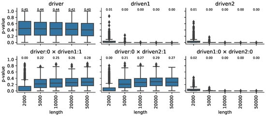
Figure 2.
Markov property of Alice (driver) Bob and Barry Driven1,2 (upper row) and the joints (lower row) for different sample sizes. After the colon symbol, the lag is indicated, and the × symbol stands for the joint of the two series. The number over the boxes indicates the median value.
Our next example is a discrete-time, continuous recursive system, the logistic map with system noise. The recursive generation is as follows:
with randomly selected for each separate system and new system simulation. The coupling coefficient chosen to be , is the system noise. The function applies a reflective boundary condition, i.e., if q is in the interval , then q is left unchanged; otherwise, it is folded back onto the interval . In this setting, the is an autonomous system, called a driver, while, for and , both with a one-step effect propagation delay. The mutual driving is realised using and , where and drive each other, and a one-step effect propagation applies too. In all cases, to reach the stationary distribution of the system, the simulation is first run for a 100 step warm-up period, with random initial conditions drawn from the interval . The state at the end of the warm-up period is considered as the initial condition for the simulation to be analyzed. The three input series are embedded in dimensions. Local permutation is used to test the Markov property and the final p-values are calculated and presented to assess the results.
Figure 3 shows the causal connection without dynamic noise (), which means that we still have noise, but it is observational noise. We did a very rough binning, splitting the range of the variables into two bins, which of course incorporates a very big information loss, observation noise. Still, we obtain a good match with the ground truth.
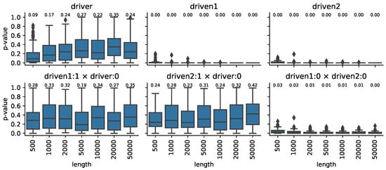
Figure 3.
Markov property of coupled logistic systems. The final p-values of the independence test for the single processes in the upper row, for the joint processes in the lower one for different sample sizes. After the colon symbol, the lag is indicated, the × symbol stands for the joint of the two series. The number over the boxes indicates the median value.
Figure 4 demonstrates similar results for system noise.
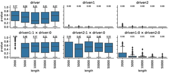
Figure 4.
Markov property of the coupled logistic systems with fixed noise. The final p-values of the independence test for the single processes in the upper row, for the joint processes in the lower one for different sample sizes. After the colon symbol, the lag is indicated, and the × symbol stands for the joint of the two series. The number over the boxes indicates the median value.
Finally, in Figure 5, we can observe the effect of different system noise for a fixed sample length (). It can be seen that the higher the noise, the more Markovian the driven chains (and their joints).
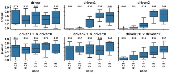
Figure 5.
Markov property of the coupled logistic systems with fixed length and various noise. The final p-values of the independence test for the single processes in the upper row, for the joint processes in the lower one for different sample sizes. After the colon symbol, the lag is indicated, the × symbol stands for the joint of the two series. The number over the boxes indicates the median value.
6.2. Real World Examples
Here, we apply the inference method to two real-world examples. The results are summarized in Figure 6.
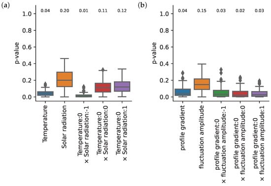
Figure 6.
Markov property of two real systems. (a) Weather data: daily mean temperature and solar irradiation at the same location for 23 years; (b) nuclear fusion data: profile gradient and fluctuation amplitude of plasma in a tokamak.
6.2.1. Weather Data
We took data N from [26] that contains the solar radiation (W/m) and the daily average temperature of the air (C) measured at the same location in Furtwangen, Black Forest, Germany, by Bernward Janzing between 1 January 1985 and 31 December 2008. The authors provide the ground truth that the temperature is driven by solar irradiation.
The data have been preprocessed to remove seasonality. The mean and std.dev. for both features and each day of the year were measured from the sample. These statistics were smoothed by a 14-day moving box window. Then, each day was z-scored by the corresponding parameters from the previous step. Our cross-correlation measurements show a peak at the 1-day lag and a second highest value at 0-day lag, although their difference is very small, making a choice between the two very uncertain.
Solar irradiation is 1-Markov, while temperature is non-Markov, indicating that solar irradiation is an autonomous process, while temperature is influenced by some other effect (see Figure 6a). We observe that setting the lag to zero makes the joint process a Markov process, and so does shifting irradiation ahead in time by one step. However, shifting irradiation backwards in time by one does not make the joint process a Markov process. Based on these results, we can not only predict the direction of causation, but also the proper lag as follows.
First, consider the fact that irradiation appears to be autonomous and temperature is not. We see that, if the lag is zero, then the joint process becomes a Markov process, implying that there is driving from irradiation to temperature. If this were the case, we would see that shifting irradiation forward in time by 1 step and testing for Markov property, jointly with the non-shifted temperature, is positive—just as the figure shows at (temperature: 0 × solar-irradiation: 1). However, if we were to shift irradiation backwards in time by 1 step and test for Markov property, jointly with the non-shifted temperature, then we would be conditioning on nodes in the graph that are colliders (see Figure 1d too), making the past and future conditionally dependent, resulting in a non-Markov process—just as we see in Figure 6a at (temperature: 0 × solar-irradiation: ). This implies that the results are in alignment with the hypothesis that there is driving from irradiation to temperate at lag zero.
From the cross-correlation plot, we saw that we also have a peak at a lag of 1. If this were the case, then the facts that irradiation appears to be autonomous, temperature does not, and (temperature: 0 × solar-irradiation: 1) is Markov would imply that there is driving from irradiation to temperature at lag 1. However, if this were the case, then (temperature: 0 × solar-irradiation: −1) should be Markov. If it is not Markov, the only reason is that external influence exists for the temperature artefact. However, this would destroy the Markov property of the two other joint processes, which is not in alignment with the results. Consequently, the high correlation at lag 1 is just an artefact, not reflecting a true causal connection.
To conclude, although we could not identify the proper lag between the time series based on their cross-correlation alone, by applying the proposed procedure, we were not only able identify the ground truth (that irradiation drives temperature), but we also managed to identify the spurious correlation at lag 1 to be an artefact. Driving with a 0-lag implies that there is instantaneous causation, which is simply “quantization error”: in reality, a change in irradiation propagates to a change in temperature over time and not instantly, but this propagation is much faster than a whole day, and since our dataset consists of daily averages, the effect seems instantaneous.
6.2.2. Plasma Fluctuation Data
As a real life application of our method, we consider two time series acquired in a fusion plasma device [27], using Beam Emission Spectroscopy measurements [28]. The first signal represents the temporal evolution of plasma density gradient (PG) while the second time trace is proportional to the strength of density fluctuations (DF) [29,30]. We can ask whether plasma fluctuations can affect the local shape of the density profile. Before applying our Markov chain test to the data, we first calculated the Pearson cross-correlation, and we found correlation between the time series. Figure 6 shows the results of the statistical testing. We assumed memory 9, and we used reference p-values from local permutations of . The test result indicates that the fluctuation amplitude (DF) can be represented as a Markov process. The profile gradient (PG) is not a Markov process either of the variously lagged joint processes. (Lags indicated in Figure 6. It fixes the time index of (PG) and shifts (DF) so that forms the joint if next to the text ’fluctuation amplitude:’ we have i). Therefore, we can conclude that the profile gradient has an external driver in addition to the fluctuations. This finding can be consistent with the picture that the plasma fluctuations are local manifestations of a turbulent plasma flow, which can certainly affect the density profile [31]. In terms of our original notations, drives . This follows from the fact that all the joint processes are non-Markov, but is, and and Z cannot be present, while there must be at least one process that drives ; in our notation, exists. Let us emphasize that this example serves demonstration purposes. It presents measurements of a single plasma discharge, and, as such, the conclusions cannot be considered as conclusive physical findings. More systematic investigations on multiple discharges are needed to establish solid plasma physics results. Note, however, that the causal relationships found in this analysis do not contradict the known physical models.
7. Discussion
Very few attempts were made, some of which were successful, to detect the hidden common drivers of stochastic dynamical systems. Our method joins these efforts and, as demonstrated, it is capable of detecting the hidden common causes (common drivers) as well as uni- or bidirectional causal relations as well as it is able to detect external influence.
The original PC algorithm developed by Pearl [2] has undergone a number of extensions and refinements relevant to the study of causal discovery from observed time series. Some notable examples include [7,13,17,20]. For more information, see the bibliography of these works and the extended surveys in [20,32]. The approach of the recently published works [13,33] is similar to the one presented in this paper. In particular, we also use a structural modeling framework, but we focus specifically on the discovery of causal relationships between pairs of systems. However, our method can be extended to the study of multiple time series by considering vector-valued observations and performing pairwise investigations for each created pair of vectors. The latter mentioned papers face the difficulty of the curse of dimensionality, as does the extension of our method. On the other hand, we have much fewer and more easily testable conditions than those postulated in [33].
In particular, the work in [33] assumes that all hidden variables are memoryless, which is a strong assumption that cannot be verified. The paper [13] removes almost all restrictions on latent processes, even allowing for contemporaneous causation, except for cyclic ones. Our method has a similar set of relaxed assumptions, but through the study of conditional dependencies, we are able to reveal mutual causal connections between observed variables in the presence or absence of hidden common causes. To some extent, the nature of the hidden common cause is also revealed, specifically whether it is memoryless.
The capabilities and limitations of causal discovery algorithms have been thoroughly investigated in seminal works such as [2,12,34,35], and more recently in [13,36]. Recent generalizations extend the labeling of the edges of classical directed acyclic graphs (DAGs), but completeness does not necessarily imply that all relations are unambiguous. Completeness means that all possible Markov equivalent maximal ancestral graph (MAGs) can be created, and no further structural information can be obtained from independence tests.
One of the most challenging problems in causal discovery is detecting the presence of a hidden common driver. There have been some attempts to address this issue (for the limitations of detecting hidden common causes, see [37]). If a method is based on the predictive causality principle or on an embedding scheme, it is unable to properly detect a hidden common driver due to inherent theoretical limitations. To the best of our knowledge, there are currently only two methods that claim to be able to detect a hidden common driver, both of which are developed for deterministic dynamic systems. Hirata’s method [38], based on the method of recurrence plots, is able to detect a hidden common driver using a series of statistical tests. However, this method often leaves the decision in a “cannot be rejected” state and is not able to provide firm conclusions in all cases. Hirata has also developed a combined method [39] to address this weakness and provide full characterization of causal relationships. It uses the recurrence plots method, comparison of the reconstructed state spaces from the observed systems, and the method of transfer entropy. The final conclusion is then drawn through majority voting of the three methods and compared with the result of the convergence cross mapping method. In contrast, Stippinger et al. [14] developed the Dimensional Causality (DC) method, which is a unified framework for investigating the causal relationships between dynamic systems. It assigns probabilities to the possible causal models, including the existence of a hidden, unobserved common driver. To the best of our knowledge, this is the first fully theoretical complete method that is able to discover the true causal model behind a pair of observed time series (without intervention) of deterministic dynamic systems. However, as demonstrated by a simple example in Section 2, the DC method cannot handle stochastic dynamic systems and fails to detect causation in the presence of noise. A recent state space reconstruction-based result (submitted) from the authors of this paper provides similar full identification of causal relationships using a proxy for entropy, the complexity of the observed time series.
We have made three assumptions in our work. First, we assumed that a continuous time process can be inferred from a discrete time series with limited resolution. Second, we assumed that the discrete time series can be well approximated by an order-p structural vector autoregressive (SVAR) model (7). This is equivalent to assuming that the entire system of processes can be approximated by an order-p Markov chain. Finally, if the processes contain continuous variables, we assumed that discretization may result in a tolerable increase in noise, which can be compensated for by creating surrogate reference data through local permutation. Coarse time resolution can lead to the observation of instantaneous (contemporaneous) causal links, as discussed in detail in [13]. In this paper, we only assume that such instantaneous connections do not exist between the observed variables, but may occur between the hidden variables and between the visible and hidden variables. We believe that this assumption is realistic, as there is some information available about the speed of information exchange between systems and the sampling resolution can be chosen accordingly. Currently, the method and the working examples use both “reject” and “cannot be rejected” side of the independence tests. The development of a complete statistical inference, probably in a Bayesian one (similar used in [14] ), is a matter of further study.
8. Conclusions
We proposed a method that is designed to identify all types of causal connections, including hidden common causes, and that is able to detect hidden external influence for correlated (scalar or vector valued) time series obtained by observing stochastic dynamic systems. This allows the detection of complex causal relationships in a nonparametric framework and makes our method a versatile tool for this task. Our method was tested on synthetic and real world datasets, demonstrating its applicability for noninterventional causal discovery. Overall, these characteristics make our method a promising solution for identifying causality in a variety of situations.
Author Contributions
Conceptualization, A.T.; methodology, A.T. and M.S.; software, M.S. and partially A.T.; validation, A.T and Á.Z.; formal analysis, A.T. and Á.Z.; writing—original draft preparation, A.T. and M.S.; writing—review and editing, A.B., Z.S. and Á.Z.; funding acquisition, Z.S. All authors have read and agreed to the published version of the manuscript.
Funding
Z.S. and A.T. was partially supported by an award from the National Brain Research Program of Hungary (NAP-B, KTIA NAP 12-2-201), Z.S. and A.T. by Hungarian National Research, Development and Innovation Fund, NKFIH under Grant No. K 135837. The authors thank the support of the Eötvös Loránd Research Network and the grant SA-114/2021.
Acknowledgments
On behalf of the Project “Identifying Hidden Common Causes: New Data Analysis Methods” (https://science-cloud.hu/projektek/rejtett-kozos-okok-felderitese-uj-adatelemzesi-modszerek, accessed on 3 February 2023), the authors thank for the usage of ELKH Cloud (https://science-cloud.hu/, accessed on 3 February 2023), which significantly helped them achieve the results published in this paper. The authors thank Zsigmond Benkő for the valuable questions and remarks with respect our work.
Conflicts of Interest
The authors declare no conflict of interest.
References
- Lloyd, G.E.R. Magic, Reason and Experience; Cambridge University Press: Cambridge, UK, 1979. [Google Scholar]
- Pearl, J. Causality, 2nd ed.; Cambridge University Press: Cambridge, UK, 2009. [Google Scholar] [CrossRef]
- Wiener, N. The theory of prediction. In Modern Mathematics for Engineers; Beckenbach, E., Ed.; McGraw-Hill: New York, NY, USA, 1956. [Google Scholar]
- Granger, C.W.J. Investigating Causal Relations by Econometric Models and Cross-spectral Methods. Econometrica 1969, 37, 424–438. [Google Scholar] [CrossRef]
- Maziarz, M. A review of the Granger-causality fallacy. J. Philos. Econ. 2015, 8, 6. [Google Scholar] [CrossRef]
- Balasis, G.; Donner, R.V.; Potirakis, S.M.; Runge, J.; Papadimitriou, C.; Daglis, I.A.; Eftaxias, K.; Kurths, J. Statistical Mechanics and Information-Theoretic Perspectives on Complexity in the Earth System. Entropy 2013, 15, 4844–4888. [Google Scholar] [CrossRef]
- Runge, J.; Bathiany, S.; Bollt, E.; Camps-Valls, G.; Coumou, D.; Deyle, E.; Glymour, C.; Kretschmer, M.; Mahecha, M.; Muñoz, J.; et al. Inferring causation from time series in Earth system sciences. Nat. Commun. 2019, 10, 2553. [Google Scholar] [CrossRef] [PubMed]
- Sugihara, G.; May, R.; Ye, H.; Hao Hsieh, C.; Deyle, E.; Fogarty, M.; Munch, S. Detecting Causality in Complex Ecosystems. Science 2012, 338, 496–500. [Google Scholar] [CrossRef]
- Takens, F. Detecting Strange Attractors in Turbulence. In Dynamical Systems and Turbulence, Warwick 1980; Lecture Notes in Mathematics; Rand, D., Young, L.S., Eds.; Springer: Berlin/Heidelberg, Germany, 1981; Volume 898, Chapter 21; pp. 366–381. [Google Scholar] [CrossRef]
- Stark, J. Delay Embeddings for Forced Systems. I. Deterministic Forcing. J. Nonlinear Sci. 1999, 9, 255–332. [Google Scholar] [CrossRef]
- Stark, J.; Broomhead, D.; Davies, M.; Huke, J. Delay Embeddings for Forced Systems. II. Stochastic Forcing. J. Nonlinear Sci. 2003, 13, 519–577. [Google Scholar] [CrossRef]
- Spirtes, P.; Glymour, C. An Algorithm for Fast Recovery of Sparse Causal Graphs. Soc. Sci. Comput. Rev. 1991, 9, 62–72. [Google Scholar] [CrossRef]
- Malinsky, D.; Spirtes, P. Causal Structure Learning from Multivariate Time Series in Settings with Unmeasured Confounding. In Proceedings of the 2018 ACM SIGKDD Workshop on Causal Disocvery, London, UK, 20 August 2018; Volume 92, pp. 23–47. [Google Scholar]
- Benko, Z.; Zlatniczki, A.; Stippinger, M.; Fabó, D.; Solyom, A.; Eross, L.; Telcs, A.; Somogyvari, Z. Complete Inference of Causal Relations between Dynamical Systems. arXiv 2018, arXiv:1808.10806. [Google Scholar]
- Lasota, A.; Mackey, M. Chaos, Fractals, and Noise: Stochastic Aspects of Dynamics; Applied Mathematical Sciences, Springer: New York, NY, USA, 2013. [Google Scholar]
- Norris, J. Markov Chains; Cambridge Series in Statistical and Probabilistic Mathematics; Cambridge University: Cambridge, UK, 1998. [Google Scholar]
- Sun, J.; Taylor, D.; Bollt, E.M. Causal Network Inference by Optimal Causation Entropy. SIAM J. Appl. Dyn. Syst. 2015, 14, 73–106. [Google Scholar] [CrossRef]
- Li, C.; Fan, X. On nonparametric conditional independence tests for continuous variables. WIREs Comput. Stat. 2020, 12, e1489. [Google Scholar] [CrossRef]
- Lundborg, A.R.; Shah, R.D.; Peters, J. Conditional Independence Testing in Hilbert Spaces with Applications to Functional Data Analysis. arXiv preprint 2021. [Google Scholar] [CrossRef]
- Guyon, I.; Janzing, D.; Schölkopf, B. Causality: Objectives and Assessment. In Proceedings of the Workshop on Causality: Objectives and Assessment at NIPS 2008, Whistler, BC, Canada, 12 December 2008; Volume 6, pp. 1–42. [Google Scholar]
- Lin, Z.; Han, F. On boosting the power of Chatterjee’s rank correlation. Biometrika 2022, asac048. [Google Scholar] [CrossRef]
- Azadkia, M.; Chatterjee, S.; Bayati, M.; Taylor, J. A Nonparametric Measure of Conditional Dependence; Stanford University: Stanford, CA, USA, 2020. [Google Scholar]
- Rényi, A. On measures of dependence. Acta Math. Hung. 1959, 10, 441–451. [Google Scholar] [CrossRef]
- Runge, J. Conditional independence testing based on a nearest-neighbor estimator of conditional mutual information. In Proceedings of the Twenty-First International Conference on Artificial Intelligence and Statistics, Lanzarote, Canary Islands, 9–11 April 2018; Volume 84, pp. 938–947. [Google Scholar]
- Wilson, D.J. The harmonic mean p-value for combining dependent tests. Proc. Natl. Acad. Sci. USA 2019, 116, 1195–1200. [Google Scholar] [CrossRef]
- Mooij, J.M.; Peters, J.; Janzing, D.; Zscheischler, J.; Schölkopf, B. Distinguishing cause from effect using observational data: Methods and benchmarks. J. Mach. Learn. Res. 2016, 17, 1103–1204. [Google Scholar]
- Hron, M.; Adámek, J.; Cavalier, J.; Dejarnac, R.; Ficker, O.; Grover, O.; Horáček, J.; Komm, M.; Macúšová, E.; Matveeva, E.; et al. Overview of the COMPASS results. Nucl. Fusion 2022, 62, 042021. [Google Scholar] [CrossRef]
- Anda, G.; Bencze, A.; Berta, M.; Dunai, D.; Hacek, P.; Krbec, J.; Réfy, D.; Krizsanóczi, T.; Bató, S.; Ilkei, T.; et al. Lithium beam diagnostic system on the COMPASS tokamak. Fusion Eng. Des. 2016, 108, 1–6. [Google Scholar] [CrossRef]
- Berta, M.; Anda, G.; Bencze, A.; Dunai, D.; Háček, P.; Hron, M.; Kovácsik, A.; Krbec, J.; Pánek, R.; Réfy, D.; et al. Li-BES detection system for plasma turbulence measurements on the COMPASS tokamak. Fusion Eng. Des. 2015, 96–97, 795–798. [Google Scholar] [CrossRef]
- Bencze, A.; Berta, M.; Buzás, A.; Hacek, P.; Krbec, J.; Szutyányi, M.; the COMPASS Team. Characterization of edge and scrape-off layer fluctuations using the fast Li-BES system on COMPASS. Plasma Phys. Control. Fusion 2019, 61, 085014. [Google Scholar] [CrossRef]
- Rudakov, D.L.; Boedo, J.A.; Moyer, R.A.; Krasheninnikov, S.; Leonard, A.W.; Mahdavi, M.A.; McKee, G.R.; Porter, G.D.; Stangeby, P.C.; Watkins, J.G.; et al. Fluctuation-driven transport in the DIII-D boundary. Plasma Phys. Control. Fusion 2002, 44, 717. [Google Scholar] [CrossRef]
- Vowels, M.J.; Camgoz, N.C.; Bowden, R. D’ya Like DAGs? A Survey on Structure Learning and Causal Discovery. ACM Comput. Surv. 2022, 55, 1–36. [Google Scholar] [CrossRef]
- Mastakouri, A.A.; Schölkopf, B.; Janzing, D. Necessary and sufficient conditions for causal feature selection in time series with latent common causes. arXiv 2020, arXiv:2005.08543. [Google Scholar]
- Zhang, J. On the completeness of orientation rules for causal discovery in the presence of latent confounders and selection bias. Artif. Intell. 2008, 172, 1873–1896. [Google Scholar] [CrossRef]
- Zhang, J. Causal Reasoning with Ancestral Graphs. J. Mach. Learn. Res. 2008, 9, 1437–1474. [Google Scholar]
- Lin, H.; Zhang, J. On Learning Causal Structures from Non-Experimental Data without Any Faithfulness Assumption. In Proceedings of the 31st International Conference on Algorithmic Learning Theory, San Diego, CA, USA, 9–11 February 2020; Volume 117, pp. 554–582. [Google Scholar]
- Liu, T.; Ungar, L.; Kording, K. Quantifying causality in data science with quasi-experiments. Nat. Comput. Sci. 2021, 1, 24–32. [Google Scholar] [CrossRef]
- Hirata, Y.; Aihara, K. Identifying hidden common causes from bivariate time series: A method using recurrence plots. Phys. Rev. E 2010, 81, 016203. [Google Scholar] [CrossRef]
- Hirata, Y.; Amigó, J.M.; Matsuzaka, Y.; Yokota, R.; Mushiake, H.; Aihara, K. Detecting Causality by Combined Use of Multiple Methods: Climate and Brain Examples. PLoS ONE 2016, 11, e0158572. [Google Scholar] [CrossRef]
Disclaimer/Publisher’s Note: The statements, opinions and data contained in all publications are solely those of the individual author(s) and contributor(s) and not of MDPI and/or the editor(s). MDPI and/or the editor(s) disclaim responsibility for any injury to people or property resulting from any ideas, methods, instructions or products referred to in the content. |
© 2023 by the authors. Licensee MDPI, Basel, Switzerland. This article is an open access article distributed under the terms and conditions of the Creative Commons Attribution (CC BY) license (https://creativecommons.org/licenses/by/4.0/).