Abstract
Misalignment is one of the most common challenges that the normal operation of journal bearings faces. This type of problem may be the result of a wide range of reasons, such as bearing wear, shaft deformation, and errors related to the manufacturing and installation process. The main undesirable consequences of the misalignment, such as pressure rise and lubricant film reduction, are concentrated on the bearing edges. Therefore, chamfering the bearing edges reduces such misalignment-related drawbacks. This work presents a novel numerical solution to the problem of finite-length journal bearing considering edge chamfering. This solution involves the determination of the levels of lubricant layer thickness and pressure distribution in addition to the journal trajectory under impact load with the related stability limits. The finite difference method is used in this solution, and the equations of motion are also solved numerically using the Runge–Kutta method. The Results of this novel analysis show that chamfering the bearing edges increases the film thickness and reduces pressure spikes associated with the system operation under the case of 3D misalignment. Furthermore, the chamfered bearing shows a wide stability range under impact loads, where the normal bearing is unstable as the critical speed increases by 26.98%, which has positive consequences on the journal’s trajectory.
MSC:
74H55; 65P40
1. Introduction
Journal bearing is the most common type of bearing as a result of its characteristics in terms of load capacity, cost of manufacturing as well as maintenance, dynamic characteristics, etc. It is used in a machine that rotates at high speeds, such as the different types of turbines (hydroelectric, steam, and gas turbines), compressors, and others. The performance of these rotating types of machinery depends to a large extent on the performance of the bearing system. The demand for high power output in today’s applications increases the rotating machinery speed, increasing the instability problems in rotors supported on such bearings. Under high speeds, the journal bearing is subjected to dynamic instability, such as oil whirl and whip [1]. Shaft whipping, or whip, means that the shaft vibrates with a constant frequency when the rotation speed is double the critical speed [2]. This vibration displaces the center of the journal from its equilibrium position. Due to unbalanced forces, the center of the journal begins to whirl from the equilibrium position in the clearance of the bearing space and may cause instability in the journal bearing. In general, considerations of stability are significant in high-speed applications.
In the aligned case, the bearing and shaft axes remain parallel, despite the high rotational speed as well as the large load. This ideal situation is perfect, but in fact, it is difficult to obtain in the case of the actual use of journal bearings. During the operation of the bearing system, the rotating shaft will be under misalignment as a result of several causes, such as its large deformation under load, manufacturing errors in the designed tolerances, asymmetricity in the bearing load, etc.
It is well known that journal bearing performance is generally affected by the degree of misalignment. Under high levels of misalignment, the lubricant layer decreases significantly at the edges, which increases the wear rate of the bearing. The presence of misalignment increases critical speed to a certain limit [3], but on the other hand, it results in a significant increase in the maximum pressure and a sharp reduction in the thickness of the lubricant layer [4,5]. In other words, misalignment reduces the load-carrying capacity of the bearing with respect to a design limit for the film thickness. Therefore, the designer needs a critical balance between the stability limits and the designed load capacity of the bearing.
One of the experimental attempts of bearing chamfering was performed by Nacy [6] in order to reduce the side flow. Bouyer and Fillon [7] solved numerically a thermo-hydrodynamic misaligned journal bearing problem. They proposed the use of designed defects to reduce the misalignment drawbacks where a 60% improvement in the film thickness level was obtained. Strzelecki [8] presented a solution considering bearings with a variable axial profile. The modification was only performed over the whole bearing length. Chasalevris and Dohnal [9] reduced the vibration amplitude by using variable bearing geometry. Later, Chasalevris and Dohnal [10] analyzed the problem using two partial arcs bearing adjustable dynamic coefficients and varied the geometry to improve the turbine stability limits. The effect of bearing profile was investigated by Liu et al. [11] where the study was extended to consider the elasto-hydrodynamic regime in a journal bearing. Several studies proposed chamfering the bearing edges to reduce the misalignment effects without considering its impact on the system stability [5,12].
The numerical solution of journal bearing problems to identify stability limits was largely covered over the last few decades. Majumdar and Brewe [13], for example, analyzed the stability characteristics of the rigid rotor supported by journal bearings using the finite difference method. Pai and Majumdar [14] studied the stability of journal bearings under dynamic loads. Qiu and Tieu [15] solved Reynolds equation using the finite difference method under static loads where the static and dynamic characteristics as well as the stability limits of the bearings were calculated considering the effect of misalignment. Tieu and Qiu [16] compared the stability contour found based on linear theory and from a nonlinear simulation. Their results showed that the critical speeds were the same for the linear and nonlinear approaches. However, the trajectories of the journal under dynamic load were slightly different in the two solutions. In their paper, neither the effect of misalignment nor the bearing modification were considered in the solution. Papadopoulos et al. [17] investigated the stability limits of the bearings, considering the effect of misalignment. Boukhelef et al. [18] used the finite element method to calculate the dynamic and static characteristics as well as the stability of journal bearings. Nicoletti [19] used an optimization method to find bearing profiles that ensure better stability margins of rotor-bearing systems. Results showed the possibility of finding the required shapes for the bearing that considerably improved the stability margins for the case of perfectly aligned bearings. Mehrjardi et al. [20] analyzed the journal bearing stability using the 4th-order Runge–Kutta method to solve the equations of motion. Results showed that stability was enhanced by increasing the amount of bearing non-circularity. Jain and Sharma [1] analyzed journal bearings’ linear and nonlinear motions based on a numerical simulation for the journal center path. Song et al. [21] studied the influence of shaft and bearing shape errors on the stability of journal bearings. Yadav et al. [22] investigated the stability of the journal bearing using the 4th-order Runge–Kutta method in order to analyze the dynamic stability of the system. Dyk et al. [23] used an analytical method to calculate the bearing dynamic coefficients but with a limited π–film condition. Sun et al. [24] studied the effect of shaft shape errors on the dynamic characteristics of journal bearings and analyzed the stability of cylindrical journal bearings. It was found that when the shaft shape errors existed, there was a new threshold rotating speed of the system. Visnadi and Castro [25] investigated the effect of bearing clearance on the stability of short journal bearings, and the results showed that the variance in bearing clearance influenced the stability threshold. Zhang et al. [26] studied the effect of misalignment on the dynamic characteristics of journal bearings. Li et al. [27] investigated the effect of cylindricity error on the dynamic coefficients and stability of the system.
It is clear from the aforementioned work that bearing stability is quite an important subject for industry. This importance comes from today’s applications that require high levels of speed which raises problems of stability. The finite-length journal bearing is the most common type of this bearing in the industry [28]. This type generally requires numerical solutions to predict the system’s characteristics accurately. However, despite the extensive previous work on this topic, a comprehensive study for the effects of a chamfer on the stability of journal bearings is still required. Such a study will provide a clear picture of the influence of chamfer parameters on the stability of the journal bearing.
Therefore, in the present work, a numerical solution is used to solve the hydrodynamic problem of finite-length journal bearings to predict the stability limits of the rotor under classical hypotheses of hydrodynamic lubrication. Furthermore, a 3D misalignment model is incorporated into the solution scheme in order to evaluate the misalignment effects on the stability of the chamfered bearings. In addition, the presence of the dynamic load will also be examined in order to determine the journal trajectories and their reflections on the stability of the system. The stability of the journal bearing is analyzed by calculating the dynamic characteristics of the bearing, which are calculated from the pressure distribution by solving the Reynolds equation. In this work, the Reynolds equation is solved numerically by using a finite difference method. All the parameters are used in the dimensionless form in order to generalize the results. The stability analysis is performed for three cases: aligned, misaligned, and chamfered bearings. The dynamic behavior is solved by determining the journal trajectory (position of journal center) as the trajectory gives a better understanding of the dynamic behavior of the journal bearing system. The equations of motion are solved numerically by using the Runge–Kutta (4th-order) method to find the trajectories of the journal in the case of aligned bearing and chamfered bearing profiles.
2. The Mathematical Problem
The complete solution of the hydrodynamic lubrication problem of journal bearings in this work involves the following steps:
- Setting the main governing equations, i.e., the Reynolds and the film thickness equations.
- Deriving the equations required to calculate the dynamic coefficients.
- Incorporating the 3D misalignment and the chamfer equations into the film thickness equation.
- Setting the equations of motion in order to determine the critical speed and the journal trajectory equations.
- Performing a numerical solution using a finite difference method to determine the film thickness, pressure distribution, and dynamic coefficients.
- Using the Runge–Kutta method to solve the equations of motion required to determine the journal trajectory under impact loads.
3. Governing Equations
The problem of hydrodynamic journal bearings requires the solution of the Reynolds equation and the description of the film thickness function, which are represented by Equations (1) and (2), under the classical hypotheses of the isothermal hydrodynamic lubrication regime [29,30]:
where : density, h: film thickness, : viscosity, p: pressure, : mean velocity, : journal velocity, : bearing velocity, t: time, c: radial clearance, : eccentricity ratio, and : attitude angle.
The bearing is stationary when , and . The squeeze term is equal to zero () for the steady-state case, and is constant for incompressible flow.
The pressure distribution is obtained by solving Equation (2) using appropriate boundary conditions, such as the Reynolds boundary method, which requires [31]:
at
at
The cavitation angle can be determined by using an iteration method [31,32]. This involves finding the negative pressure resulting from the solutions of the Reynolds equation, starting from the last node before the boundary at the exit in the circumferential direction, setting its value to zero, and resolving the Reynolds equation based on this new condition. This process continues until all the pressure values become positive (or zero). It is worth mentioning that the identification of the locations of the negative pressure is performed in both directions .
The Reynolds equation will be written in a dimensionless form for the purpose of the generality of the results.
The introduced dimensionless variables are:
where L: bearing length, R: radius, P: dimensionless pressure, p: pressure, : the atmospheric pressure, and H: dimensionless film thickness.
Therefore, Equation (1) in a dimensionless form becomes:
where
Equation (2) describes the lubricant film thickness, and it can be written in a dimensionless form as
The dimensionless load components can be calculated by integrating the pressure field over the bearing surface domain [29]:
The integration can be evaluated up to the cavitation zone or continuing to include all the nodes. The pressure is zero over this zone, so the numerical integration will not be affected. However, the calculation time can be reduced by limiting the integration to consider only the area where the pressure is generated.
Therefore, the total load is:
where
The attitude angle, defined as the angle between the line of centers and the load (W) direction, can be written as [33]:
In the dynamic analysis, the nonlinear hydrodynamic fluid film forces should be linearized around a shaft-steady position allowing the determination of four stiffness and four damping coefficients. These coefficients are necessary for investigating the stability of the shaft around the equilibrium position. These coefficients are symbolized, respectively by , , , , , , , and .
4. Calculation of Dynamic Characteristics
The stiffness and damping coefficients equations are derived in this section, based on the following time-dependent on the Reynolds equation.
Under the dynamic condition, the equation of film thickness is [34]
Differentiation of Equation (9) with respect to time yields
Substituting Equation (11) into Equation (9) gives
Equation (12) can be written in a dimensionless form as
where ,
It is worth mentioning that the x-axis is downward in the work of Lund and Thomson [34] and the same direction for this axis is considered in this section. However, the results of the dynamic coefficients are reversed in order to be consistent with the adopted system of coordinates in this work.
The resultant forces are a function of ,,, and as given by [33,34]:
where the resultant force is
The dynamic coefficient and matrices (stiffness and damping) can be written in the following form [35]:
The stiffness coefficients are written using the form suggested by [34]:
Similarly, the damping coefficients are
Therefore, the differentiation of Equation (3) and using Equations (15) and (16) yields
where
In the same way, the damping coefficients are determined from the integration of the pressure derivatives:
where
The derivatives related to the calculation of the coefficients are evaluated as follows:
The differentiation with respect to and Y yields
Similarly, the differentiation with respect to and gives
Equations (19)–(22) will be solved numerically in order to find the pressure derivatives required to calculate the dynamic coefficients , , , , , , and . The resulting general equation after discretizing these equations is given in the section of the numerical solution.
5. Stability of Journal Bearing
The shaft whirl happened to the journal center around its equilibrium position at a certain angular speed [16]. The system is stable if the critical speed (function of dynamic coefficients) is higher than the journal rotating speed. The critical speed can be determined by solving the rotor equations of the motion. The equations of motion for a rigid unbalanced rotor supported by two bearings that are shown in Figure 1 are [36].
 where [16] and represent the external loads, is the unbalanced force, while the bearing forces are represented by .
Figure 1.
Bearing system: (a) side view of the journal bearing; (b) supported rotor [36] edited.
The axes of whirling of the journal center at an angular speed around its equilibrium position are (,) as shown in Figure 1a.
Equations (23) and (24) can be written as
where
The following function is used in this paper to describe the external force as an impact load [16]:
and
Neglecting the external and unbalanced forces, in order to determine the critical speed, the standard linear equations are
The bearing forces can be expressed for small displacement around the equilibrium position by [16]
Substitution of Equations (30) and (31) in Equations (28) and (29) gives
The solution for the above equations is [37]
Substitution of these solutions in Equations (32) and (33) yields
where
The critical speed () is
6. The Misalignment Effects
The model of misalignment used in the current investigation is essentially adopted from a previous work of one of the authors of this paper [30], where a detailed illustration of the misalignment model can be found. A schematic drawing for the 3D misalignment model is illustrated in Figure 2. The use of the 3D model gives a more realistic representation of the shaft axis deviations. The deviations (dimensionless) along the bearing length in both directions (horizontal and vertical) are
where , and .
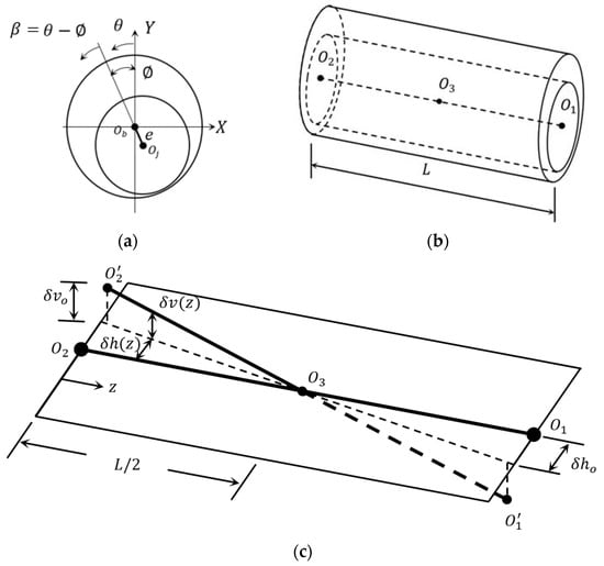
Figure 2.
Schematic drawing illustrates: (a) side view of aligned bearing, (b) 3D aligned bearing, and (c) misalignment model [30].
The attitude angle and the eccentricity in the case of the misaligned bearing are functions of z position, which can be given by [30]
where and are the eccentricity distance and the attitude angle at the middle of the bearing width respectively. The eccentricity ratio is determined by dividing the eccentricity, by the radial clearance, . The effect of misalignment is incorporated into the film thickness, Equation (4), by calculating the new radial gap between the journal and the bearing at any position. This calculation can be achieved by determining the attitude angle and the eccentricity ratio corresponding to the misalignment parameters given by Equation (39).
7. Profile Modification of the Bearing
The chamfered bearing is schematically illustrated in Figure 3. More detail about this modification can be found in the previous reference [12]. The gap in the circumferential direction resulted from the bearing chamfer, which is a function of z along the bearing length as [12]
The dimensionless parameters and in these equations are
The values of these parameters are used to evaluate the adopted method of bearing chamfering. Scaling the design parameters to the clearance, , and the bearing length, , gives a clearer picture of the amount of change in terms of the bearing design parameters.

Figure 3.
Bearing modification: (a) 3D unmodified bearing, (b) 3D modified bearing, and (c) schematic drawing of a chamfered bearing.
The coupling of Equations (4), (38), and (40) gives the total gap between the misaligned shaft and the chamfered bearing, and the resulting gap is used in the analyses of static and dynamic characteristics described previously.
8. Numerical Solution
The dynamic coefficients are calculated numerically by solving the governing equations (film thickness equation, Reynolds equation, and the equations related to the misalignment and modification of the bearing) mentioned previously. After determining the dynamic coefficients, the equations of motion used to determine the stability limits and the journal trajectory are solved numerically using a fourth-order Runge–Kutta method. The solution plane is assumed to be a rectangle that contains nodes distributed in axial and circumferential directions. The Gauss–Sedial method is used to determine the pressure distribution using the successive over-relaxation method to reduce the number of iterations.
Discretizing the governing equations gives the following equations:
where , , , , and are the mesh steps.
The oil film thickness in terms of position is
More details about the discretizing scheme can be found in [5,30].
The convergence of the numerical solution is achieved by satisfying the convergence of the pressure values, which is given by and also by satisfying the load convergence criterion.
After obtaining the convergence of the solution based on the pressure, the bearing forces in both directions are calculated numerically, and the resultant hydrodynamic load can be calculated. The resulting load is then compared with the actual applied load to achieve an accuracy limit of . If the difference is not within this limit, the eccentricity ratio is updated, and the pressure distribution is calculated again. This process continues until the load (as well as the pressure) convergence is obtained. This load corresponds to an eccentricity ratio of 0.6 in the perfectly aligned case. A flow chart for the solution steps is shown in Figure 4. After that, the dynamic coefficients can be calculated, and the equations of motion are solved using the Runge–Kutta method.
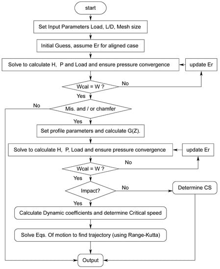
Figure 4.
Flowchart of the solution steps.
The numerical solution of Equations (19)–(22) is required to calculate the dynamic coefficients. Discretizing these equations gives the following general equation, which is also solved numerically as explained above, to find the corresponding pressure derivative ():
where
The right side of Equations (19)–(22) can be determined numerically as follows:
The solution of the hydrodynamic lubrication problem with the consideration of the 3D misalignment and the bearing chamfer has faced considerable challenges. Examples of that are the determination of the cavitation zone boundaries, which requires an iterative solution, and derivation of the required equations to calculate the dynamic coefficients with the consideration of the misalignment and the chamfer models. Furthermore, the relaxation factor that achieved a fast convergence for the pressure distribution should be determined in addition to the finding of the faster algorithm for the load conveyance.
9. Results and Discussions
In the beginning, a series of tests are performed to find the optimal number of mesh points for this analysis as well as the number of time steps. Furthermore, the stiffness coefficients are compared with the results of reference [10] for the purpose of verification. Table 1 shows this comparison using two values of the Summerfield number, where . The agreement is excellent at the relatively low and high values of the Summerfield number.

Table 1.
Verification of the current work.
The effect of the bearing chamfer on the pressure distribution is shown in Figure 5 for a finite-length bearing where , using different misalignment and modification cases. The pressure distribution for the aligned case () is shown in Figure 5a where uniform and symmetric distribution about the line (half of the bearing length) is the distinguishing feature of this case. Figure 5b,c show the results for the cases and .58, respectively, where the pressure increases significantly due to these levels of misalignment and also loses its symmetricity about the middle of the bearing along the z direction. Introducing the chamfer at the bearing edges for the last extreme case (.58) reduces the pressure spikes significantly as shown in Figure 5d,e. The chamfer parameters for these two figures are and respectively. It can be seen that when the pressure becomes closer to the aligned case distribution where the asymmetric distribution due to misalignment is overcome in addition to the reduction in its maximum value [12]. The maximum pressure is reduced by 26.34% due to the bearing chamfer compared to the misalignment case.
The corresponding film thickness of these cases is shown in Figure 6, where the chamfer improves the minimum film thickness by almost three times.

Figure 5.
Effect of bearing chamfer on the dimensionless pressure distribution (L/D = 1.25). (a) , (b) , (c) , (d) case (c) with chamfer () and (e) case (c) with chamfer ().

Figure 6.
Three-dimensional film thickness distribution (L/D = 1.25). (a) , (b) , and (c) Case (b) with chamfer ().
10. Effect of the Chamfer on the System Stability
As explained in the previous section, the misalignment has significant negative sequences on the system performance. The chamfer has shown a very clear positive effect on the levels of film thickness, the maximum pressure value, and the shape of the distribution. The results shown in this section focused on examining the chamfer effects on the system stability, which involve both the critical speed limits and the journal trajectory under impact loads. The chamfer effect on the critical speed is shown in Table 2 for the extreme case of misalignment where and chamfer parameters of .
Table 2.
Dimensionless critical speed and equivalent stiffness for different cases.
The critical speed of the aligned case is 2.678, and the corresponding critical speed for the misaligned case is 3.918. This increase in the critical speed is actually not beneficial as the misalignment increases the maximum pressure and reduces the minimum film thickness to an extremely thin level, as explained previously. Therefore, introducing the bearing edge chamfer should find a balance between the improvement in the pressure value (and the shape of distribution) and the film thickness levels and the improvement in the critical speed. Figure 7 gives a clearer picture of this outcome, whereas Figure 7a shows the effect of the chamfer parameter on the critical speed and the maximum pressure values. It can be seen that when the maximum pressure reduced significantly in comparison with the case of misalignment without chamfer (). The corresponding critical speed is also decreased over this range of but it is still larger than the critical speed of the aligned case (see previous table). When the critical speed starts to increase, but the corresponding maximum pressure also increases, which represents a drawback for the chamfer. The same behavior can be seen in Figure 7b, where the corresponding values for Hmin are illustrated (the critical speed values are repeated again for the purpose of clarity). This behavior can be explained as follows: for the misaligned case (the perfectly aligned bearing is a rarely existing case in practical applications of this type of bearing), the shaft is inclined due to misalignment, which reduces the gap between the shaft and the chamfered bearing close to the bearing edge. This situation helps generate the pressure between the two surfaces, i.e., the modified part of the bearing will support the load. On the other hand, as the chamfer height increases, the modified part will not significantly participate in supporting the load, which means that the bearing becomes shorter, which requires the pressure to be larger to support the same applied load.
It can be seen that for the chamfered bearing under the misalignment condition, when the critical speed is increased by 26.98% compared to the aligned case. The chamfered bearing will therefore operate in a stable condition over a wider range of speed compared with the unchamfered bearing. Keeping in mind the previously mentioned improvement in performance, such a gain in critical speed represents an additional benefit and an important step in the right direction. This means, in other words, that decreasing the maximum pressure and increasing the minimum film thickness can maintain an acceptable improvement in the critical speed when the misaligned bearing is chamfered.
The variation in the critical speed occurred due to the misalignment, and the bearing chamfer is a result of the change in the dynamic coefficients of the bearing system. The dynamic coefficients for the cases illustrated above are shown in Figure 8. Figure 8a,b show the variations in the stiffness and damping coefficients, respectively. The results in Figure 8 illustrate that the chamfer returns, to some extent, the values of the coefficients back towards their values in the perfectly aligned case.

Figure 7.
Effect of chamfer parameter A on the dimensionless (a) critical speed and Pmax and (b) critical speed and Hmin. (B = 0.25, L/D = 1.25, ).

Figure 8.
Variation of the dynamic coefficients due to misalignment and the bearing chamfer: (a) stiffness coefficients and (b) damping coefficients. ( and for the modified and chamfered cases: , ).
When the journal is hit with an impact hummer, impulse force is applied to the rotor. The trajectory of a journal relative to this force can reflect the stability of the system. The journal trajectories under impact load for the unchamfered and chamfered bearings are illustrated in Figure 9, where , = 0.6, and in the case of the chamfered bearing. In Figure 9a, the value of speed is 2500 rpm which is less than the critical speed of the unchamfered bearing. It can be seen that the journal returns to its steady-state position after its deviation due to the impact load. This case represents a stable condition. Similar behavior can be seen on the right side of this figure for the chamfered bearing, as the rotation speed is also less than its critical speed. Figure 9b shows the trajectories when the journal speed is 2.67 (5664.61 rpm), which is equal to the critical speed of the unchamfered bearing. It can be seen that at this speed, the shaft of the unchamfered bearing continues to rotate around its steady-state position on the same orbit. This trajectory represents the critical case. On the other hand, the chamfered bearing, where its journal trajectory is illustrated on the right side of Figure 9b, is stable, and the shaft returns to its original location.
In Figure 9c, is 3.40 (6055.17 rpm), which is equal to the critical speed of the chamfered bearing system. The shaft of the chamfered bearing rotates around the equilibrium position in a fixed orbit, but the chamfered journal bearing is unstable as the amplitude increases with time and finally reaches the bearing wall. It is clear that chamfering the bearing increases the speed range in which the journal can rotate in stable conditions under impact load.
The trajectory of the 3D misalignment journal under impact load and the bearing chamfer is an extremely complex case as the position of the journal center varies along the bearing length, which requires a different method of solution as the equation of motion should consider this variation. However, the authors intend to address this case in the next work on this path of research.


Figure 9.
Effect of chamfer on the journal trajectory subjected to an impact load. Left: unchamfered, right: chamfered. (a) 2500 rpm, (b) 5664.61 rpm, (c) 6055.17 rpm. (L/D = 1.25, = 0.6).
11. Conclusions
In this paper, the stability of chamfered journal bearings and the journal trajectory under an impact load are investigated in detail using a novel numerical approach. Chamfering the bearing profile and its consequences on the general performance of the journal bearing system is also presented. Furthermore, a 3D misalignment model is incorporated into the analysis. It has been found that the misalignment increases the levels of and decreases significantly, and the chamfer helps to reduce and increase . In addition, the chamfer has obvious influences on , although the (in the case of misalignment) is greater than those of the corresponding aligned case (46.28% greater in the extreme misaligned case), and there are clear drawbacks of the misalignment on and . Therefore, the chamfer is used to ensure acceptable levels of and and also to maintain the stability of the journal bearing. The chamfered bearing is stable within a range of speed in which the non-chamfered bearing is unstable. This represents an important outcome as the stability of the system is also improved in addition to the previous benefits of the chamfer, which are the reduction in and the increase in . The trajectories of the journal center under impact load for the chamfered and unchamfered bearings provide a clearer understanding of the response of the system under dynamic load. It can be concluded that the bearing edge modification has significant advantages in designing the journal bearing, such as increasing the minimum film thickness, reducing the maximum pressure resulting from the misalignment, and improving in the stability of the system under impact loads.
Author Contributions
Formal analysis, Investigation, Writing—review and editing, H.U.J.; Methodology, Resources, H.S.S.; Formal analysis, Writing—review and editing, O.I.A.; Recourses, Funding Acquisition, A.N.J.A.-T.; Validation, Writing—review and editing, M.S.A.; Writing—review and editing, Supervision, A.R.; Writing—review and editing, Z.A.A.-D. All authors have read and agreed to the published version of the manuscript.
Funding
This research received no external funding.
Data Availability Statement
The study did not report any data.
Conflicts of Interest
The authors declare no conflict of interest.
References
- Ruggiero, A.; D’Amato, R.; Magliano, E.; Kozak, D. Dynamical Simulations of a Flexible Rotor in Cylindrical Uncavitated and Cavitated Lubricated Journal Bearings. Lubricants 2018, 6, 40. [Google Scholar] [CrossRef]
- Frene, J. Hydrodynamic Lubrication Bearings and Thrust Bearings; Elsevier: Amsterdam, The Netherlands, 1997. [Google Scholar]
- Rao, T.V. Stability Characteristics of Misaligned Journal Bearing. Adv. Vib. Eng. 2012, 11, 362–369. [Google Scholar]
- Sun, J.; Gui, C.; Li, Z.; Li, Z. Influence of Journal Misalignment Caused by Shaft Deformation Under Rotational Load on Performance of Journal Bearing. Part J J. Eng. Tribol. 2005, 219, 275–283. [Google Scholar] [CrossRef]
- AL-Dujaili, Z.A.; Jamali, H.U.; Al-Saadi, M. Effect of Axial Profile Modification on the Characteristics of a Finite Length Misaligned Journal Bearing. IOP Conf. Ser. Mater. Sci. Eng. 2020, 671, 012021. [Google Scholar] [CrossRef]
- Nacy, S.M. Effect of chamfering on side-leakage flow rate of journal bearings. Wear 1997, 212, 95–102. [Google Scholar] [CrossRef]
- Bouyer, J.; Fillon, M. Improvement of the THD Performance of a Misaligned Plain Journal Bearing. J. Tribol. 2003, 125, 334–342. [Google Scholar] [CrossRef]
- Strzelecki, S. Operating characteristics of heavy loaded cylindrical journal bearing with variable axial profile. Mater. Res. 2005, 8, 481–486. [Google Scholar] [CrossRef]
- Chasalevris, A.; Dohnal, F. A journal bearing with variable geometry for the suppression of vibrations in rotating shafts: Simulation, design, construction and experiment. Mech. Syst. Signal Process. 2015, 52–53, 506–528. [Google Scholar] [CrossRef]
- Chasalevris, A.; Dohnal, F. Enhancing stability of industrial turbines using adjustable partial arc bearings. J. Phys. Conf. Ser. 2016, 744, 12152. [Google Scholar] [CrossRef]
- Liu, C.; Zhao, B.; Li, W.; Lu, X. Effects of bushing profiles on the elastohydrodynamic lubrication performance of the journal bearing under steady operating conditions. Mech. Ind. 2019, 20, 207. [Google Scholar] [CrossRef]
- Jamali, H.U.; Sultan, H.S.; Senatore, A.; Al-Dujaili, Z.A.; Jweeg, M.J.; Abed, A.M.; Abdullah, O.I. Minimizing Misalignment Effects in Finite Length Journal Bearings. Designs 2022, 6, 85. [Google Scholar] [CrossRef]
- Majumdar, B.C.; Brewe, D.E. Stability of a Rigid Rotor Supported on Oil-Film Journal Bearings under Dynamic Load. In Proceedings of the National Seminar on Bearings, Madras, India, 17–18 September 1987. [Google Scholar]
- Pai, R.; Majumdar, B.C. Stability of submerged four-lobe oil journal bearings under dynamic load. Wear 1992, 154, 95–108. [Google Scholar] [CrossRef]
- Qiu, Z.L.; Tieu, A.K. Misalignment Effect on the Static and Dynamic Characteristics of Hydrodynamic Journal Bearings. J. Tribol. 1995, 117, 717–723. [Google Scholar] [CrossRef]
- Tieu, A.K.; Qiu, Z.L. Stability of Finite Journal Bearings–-from Linear and Nonlinear Bearing Forces. Tribol. Trans. 1995, 38, 627–635. [Google Scholar] [CrossRef]
- Papadopoulos, C.A.; Nikolakopoulos, P.G.; Gounaris, G.D. Identification of clearances and stability analysis for a rotor-journal bearing system. Mech. Mach. Theory 2008, 43, 411–426. [Google Scholar] [CrossRef]
- Boukhelef, D.; Bounif, A.; Bouzid, D.A. Dynamic characterization and stability analysis of hydrodynamic journal bearing using the FEM. Mechanika 2011, 17, 503–509. [Google Scholar] [CrossRef]
- Nicoletti, R. Optimization of journal bearing profile for higher dynamic stability limits. J. Tribol. 2013, 135, 011702. [Google Scholar] [CrossRef]
- Mehrjardi, M.Z.; Rahmatabadi, A.D.; Meybodi, R.R. A comparative study of the preload effects on the stability performance of noncircular journal bearings using linear and nonlinear dynamic approaches. Part J J. Eng. Tribol. 2016, 230, 797–816. [Google Scholar] [CrossRef]
- Song, M.; Azam, S.; Jang, J.; Park, S.-S. Effect of shape errors on the stability of externally pressurized air journal bearings using semi-implicit scheme. Tribol. Int. 2017, 115, 580–590. [Google Scholar] [CrossRef]
- Yadav, S.K.; Rajput, A.K.; Ram, N.; Sharma, S.C. Stability analysis of a rigid rotor supported by two-lobe hydrodynamic journal bearings operating with a non-Newtonian lubricant. Part J J. Eng. Tribol. 2019, 233, 884–898. [Google Scholar] [CrossRef]
- Dyk, Š.; Rendl, J.; Byrtus, M.; Smolík, L. Dynamic coefficients and stability analysis of finite-length journal bearings considering approximate analytical solutions of the Reynolds equation. Tribol. Int. 2018, 130, 229–244. [Google Scholar] [CrossRef]
- Sun, F.; Zhang, X.; Wang, X.; Su, Z.; Wang, D. Effects of Shaft Shape Errors on the Dynamic Characteristics of a Rotor-Bearing System. J. Tribol. 2019, 141, 101701. [Google Scholar] [CrossRef]
- Visnadi, L.B.; de Castro, H.F. Influence of bearing clearance and oil temperature uncertainties on the stability threshold of cylindrical journal bearings. Mech. Mach. Theory 2019, 134, 57–73. [Google Scholar] [CrossRef]
- Zhang, J.; Zhao, H.; Zou, D.; Ta, N.; Rao, Z. Comparison study of misalignment effect along two perpendicular directions on the stability of rigid rotor-aerostatic journal bearing system. Part J J. Eng. Tribol. 2020, 234, 1618–1634. [Google Scholar] [CrossRef]
- Li, B.; Zhou, D.; Ogrodnik, B.; Xu, W. Effect of journal cylindricity error with saddle or drum distribution on the performance of hydrodynamic journal bearing systems. Part J J. Eng. Tribol. 2020, 234, 1092–1105. [Google Scholar] [CrossRef]
- Szeri, A.Z. Fluid Film Lubrication, Theory and Design; Cambridge University Press: Cambridge, UK, 2005. [Google Scholar]
- Chasalevris, A.; Sfyris, D. Evaluation of the Finite Journal Bearing Characteristics, Using the Exact Analytical Solution of the Reynolds Equation. Tribol. Int. 2013, 57, 216–234. [Google Scholar] [CrossRef]
- Jamali, H.; Al-Hamood, A. A New Method for the Analysis of Misaligned Journal Bearing. Tribol. Ind. 2018, 40, 213–224. [Google Scholar] [CrossRef]
- Hamrock, B.J. Fundamentals of Fluid Film Lubrication; McGraw-Hill: New York, NY, USA, 1991. [Google Scholar]
- Harnoy, A. Bearing Design in Machinery: Engineering Tribology and Lubrication, 1st ed.; Marcel Dekker: New York, NY, USA; Basel, Switzerland, 2002. [Google Scholar]
- Feng, H.; Jiang, S.; Ji, A. Investigation of the Static and Dynamic Characteristics of Water-Lubricated Hydrodynamic Journal Bearing Considering Turbulent, Thermo-hydrodynamic and Misaligned Effects. Tribol. Int. 2019, 130, 245–260. [Google Scholar] [CrossRef]
- Lund, J.W.; Thomsen, K.K. A Calculation Method and Data for the Dynamic Coefficients of Oil-Lubricated Journal Bearings; ASME: New York, NY, USA, 1978. [Google Scholar]
- Someya, T. Journal Bearing Databook; Springer: Berlin/Heidelberg, Germany, 1989. [Google Scholar]
- Shi, Y.; Li, M. Study on nonlinear dynamics of the marine rotor-bearing system under yawing motion. J. Phys. Conf. Ser. 2020, 1676, 012156. [Google Scholar] [CrossRef]
- Nicholas, J.C. Hydrodynamic Journal Bearings–Types, Characteristics and Applications. In Proceedings of the Mini Course Notes–Vibration Institute, 20th Annual Meeting, St. Louis, MO, USA, 25–27 June 1996. [Google Scholar]
Disclaimer/Publisher’s Note: The statements, opinions and data contained in all publications are solely those of the individual author(s) and contributor(s) and not of MDPI and/or the editor(s). MDPI and/or the editor(s) disclaim responsibility for any injury to people or property resulting from any ideas, methods, instructions or products referred to in the content. |
© 2023 by the authors. Licensee MDPI, Basel, Switzerland. This article is an open access article distributed under the terms and conditions of the Creative Commons Attribution (CC BY) license (https://creativecommons.org/licenses/by/4.0/).