Abstract
The transmission lines of an electricity system are susceptible to a wide range of unusual fault conditions. The transmission line, the longest part of the electricity grid, sometimes passes through wooded areas. Storms, cyclones, and poor vegetation management (including tree cutting) increase the risk of cross-country faults (CCFs) and high-impedance fault (HIF) syndrome in these regions. Recognizing and classifying CCFs associated with HIF syndrome is the most challenging part of the project. This study extracted signal characteristics associated with CCF and HIF syndrome using the Tunable Q Wavelet Transform (TQWT). An adaptive tunable Q-factor wavelet transform (TQWT) based feature-extraction approach for CCHIF fault signals with high impact, short response period, and broad resonance frequency bandwidth was presented. In the first part, the time–frequency distribution of the vibration signal is used to determine the distinctive frequency range. Adaptive optimal matching of the impact characteristic components in the vibration signal was achieved by optimizing the number of decomposition layers, quality factor, and redundancy of TQWT based on the characteristic frequency band. In the last, the TQWT inverse transform was utilized to recreate the best sub-band to boost its weak impact characteristics. The effectiveness of the approach is confirmed by simulation and experimental findings in signal processing. The best decomposition level for signature features that can be extracted has been decided by Minimum Description length (MDL). The IEEE 39-bus system is used to test the suggested approach with reactor switching and the Ferranti effect.
Keywords:
cross-country high impedance fault; jellyfish; fault detection; Tunable Q Wavelet transform; graph theory MSC:
65k99; 90c99; 68T07
1. Introduction
The double-circuit transmission line’s (DCTL) protection is multi-dimensional in a transmission line due to the influence of mutual coupling. Inter-circuit faults (ICFs), cross-country faults (CCFs), and evolving faults (EVFs) are more likely to occur. The protection of a DCTL is multi-faceted and predominance because the conductors have a particular physical geometry. The identification and categorization of ICFs and CCFs through the use of artificial neural networks (ANN) may be found in [1] and investigations that provide a detailed description of differential relaying techniques for CCFs are described in [2]. It has been reported that CCFs affect the distance-relaying topology on a transmission system, with 132 kilovolts reported in [3]. The zone-I in the distance relaying strategy for grounded CCFs and unearthed CCFs is shown in [4,5], respectively. There is interference with the effectiveness of the distance relaying plan because the CCF contains faults in two places in contrasting periods. The evolving fault (EVF) also involves primary and secondary faults at various periods during fault initiation [6]. An algorithm built on the discrete wavelet transform (DWT) and ANN has been explained in detail for the location of the shunt issue, incorporating CCFs and EVFs in a specific-circuit transmission line (SCTL) in [7].
An adaptive differential relay strategy for CCFs and CT saturation-based approach that uses continuous wavelet transform is discussed in [8]. In [9], the author explains a novel relaying technique for detecting multiple locations (MLFs) in series-compensation DCTL. The specific localizations of MLFs in series-compensation of DCTL lines with the utilization of ANN as explained in [10]. In a case study on the Chhattisgarh state transmission system’s 400 kV DCTL for CCFs and converting faults utilizing real-time data, there have been reports of a digital simulator based on ANN in [11,12]. A method for detecting and classifying CCFs based on maximal overlap reports of the discrete wavelet transform known as MODWT can be found in [12]. These schemes do not consider the high-impedance fault (HIF). The method of high-impedance arcing fault identification based on a DWT analysis of a 154-kV transmission line in Korea is presented in reference [13]. The electromagnetic interference around the power line was analyzed by utilizing an experimental decomposition mode in a mixture with methods of quantile regression that have been informed for tree-based models for detecting HIFs [14]. There has been the development of an analytic model for HIF analysis. The model using an electric arc reflection factor is explained in [15].
Recognition of High-Intensity Interrupting Events (HIFs) in power transmission utilities in [16] illustrates the application of ANN to nonlinear loads on a 110-kV transmission line. Models based on field research have been built and created to locate HIFs [17]. Constraints that are distributed evenly transmission model for the detection and categorization of high-frequency interference lines as demonstrated in [18], as an example. An issue with the lack of synchronization in a double-fed 345-kilovolt transmission, the location identification for HIFs, is explained in [19]. An assessment of the HIF in real-time recognition utilizing DWT in the EHV transmission network has been observed in [20]. A technique based on the cumulative standard deviation sum [21] illustrates the detection and classification of high resistance problems. Classifying HIFs within a unified power flow conditioner (UPFC) performed DCTL compensation with differential power has been documented in reference [22]. An additional consideration, based on alienation, of [23] demonstrates the use of voltage indications for fault detection and categorization. It has been stated in [24] that a HIF fault-locating system for series-compensation transmission lines [25] details a digital distance-relaying technique that can be used when transmission lines develop problems with high resistance. An algorithm based on neuro wavelets for identification of the use of high-intensity fields (HIFs) in extra-high-voltage (EHV) transmission networks is referred to as seen in reference [26]. It is demonstrated in [27] how HIF detection can be carried out in transmission lines by using a distance relay. The transformation of boundary wavelets has been utilized in detecting HIF [28] and faults in distribution networks in the presence of scattered generational sources. It was reported in [29] that they used a data mining-driven wavelet transform. It has been informed that there was an experimental case study of simultaneous faults inside a DCTL [30]. In addition to that, these strategies cannot work in the example of a DCTL due to the effect of mutual coupling as well as the complicated characteristics of CCF associated with HIF syndrome. Identifying and characterizing CCF-HIFs as having HIF syndrome is essential to prevent any problems with the long-distance relay.
A tunable Q-factor wavelet transform is flexible in detecting signals’ disturbances and efficiently extracts the signal’s fundamental frequency component. This made researchers use extensive fault diagnosis algorithms. Thirumala et al. proposed a Power Quality Disturbances diagnosis method using a Tunable Q-factor wavelet transform and Support Vector Machine classifier, which is discussed in [31]. A TQWT-based bearing fault identification in time-varying fields has been proposed in [32]. TQWT has also been implemented to detect train axle bearings faults [33]. Zhang et al. presented a method to identify faults in a planetary gearbox [34]. Knowledge-Based Neural Network and TQWT-based method diagnosis of Power Quality Disturbances are discussed in [35]. In this paper, the AdaBoost method is used to classify fault zone, as this algorithm has more accuracy than other algorithms.
In this paper, the TQWT-based normalized energy values are used to come up with a way to find and classify faults in the case of cross-country faults with HIF syndrome. It is the first time TQDWT has been used to find and classify cross-country faults in transmission lines with HIF syndrome. In this research work, an IEEE 39 bus network has been modeled utilizing the software MATLAB/Simulink through an ideal HIF model to recreate a typical fault condition like CCF-HIFs. The voltage and voltage signals are monitored at the bus or node sending them. The TQWT’s analysis of the lines is also being carried out. Since the TQWT may be tweaked and built on the oscillatory behavior of the signal being applied, it has been employed for signal processing. TQWT is built on a real-valued scaling coefficient or dilation coefficient. Its implementation uses a complete reconstruction oversampled filter bank through real-valued sampling coefficients. In addition, TQWT uses a real-valued sampling coefficient to determine the size of the window. In this research article, the method that has been suggested is to classify CCF-HIFs into the appropriate categories so that it is cleaned up as quickly as possible so that the power supply can be restored.
Significant contributions to the paper include:
This research demonstrates that the TQWT-based feature-extraction method significantly facilitates CCHIF fault signal detection, classification, and recognition. Feature extraction aims to reduce the number of features in a dataset by making new features from the ones already there (and then discarding the original features). Reducing the number of signal characteristics by statistical feature selection and feature elimination (TQWT) has been demonstrated to be an effective method for classifying proposed events. It also explains how to select a decomposition level that expedites and improves the accuracy of the process.
As long as the same basis function and decomposition layer number are used, the quality factor of the continuous wavelet transform remains unchanged. As long as they stay within the normalization factor’s parameters, wavelets of varying sizes can keep their energy level constant. However, the wavelet energy at each scale depends on the scale because the quality factor of TQWT is tunable. In this article, optimized values of the Quality factor (Q), Redundancy factor (r), and the number of decomposition levels (J) have been proposed to take the algorithm accurate.
Achieving system observability, which is critical for accurately assessing the power system’s state, relies heavily on the strategic placement of meters. This research provides a solution that can be used to determine the best possible sites at which to install the meters. The following clause describes such procedures: Jelly Fish is an optimization algorithm used to precisely place meters as part of this research effort.
The entropy of a signal is a useful statistical measure because it may be used to infer important information about the state of the system producing the signal. Therefore, entropy can serve as a valuable non-parametric tool for extracting features from data generated by industrial systems. The concept of normalized entropy was implemented in this study to improve fault diagnosis, especially cross-country faults with HIF syndrome. Theoretical methods for investigating the applicability of normalized entropy indices in the context of fault feature extraction from discrete data are proposed.
2. Problem Formulation
2.1. Modelling of High-Impedance Fault
HIF events are accompanied by arcing. Due to the low values of the arcing voltage, conventional overvoltage relays cannot detect these faults. Modeling of real HIF is the most sensitive part of the fault detection process, as the model should resemble and comprise all the properties of real HIF that occur in the distribution system. The basic properties of HIF that makes it distinguishable from other faults are nonlinearities, high-order harmonics, and low-frequency transients. Most HIF models are thermal models based on Cassie–Mayr thermal equations [36]. Thus, to overcome these issues Gautam et al. developed a HIF model based on practical measurements and theoretical components suggested as two DC sources Vn and Vp, connected antiparallel with two diodes Dn and Dp to generate zero periods of arcing and asymmetry. The variable resistances Rn and Rp provide nonlinearity to the Voltage–Voltage HIF behavior [37]. This preferred model in [37] has been considered the HIF model in the proposed research work. The basic diagram of the presented simplified HIF model is depicted in Figure 1.
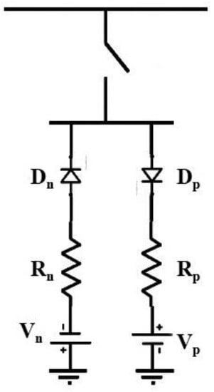
Figure 1.
Representation of Simplified HIF Model.
2.2. Tunable Q Wavelet Transform-Based Signal Decomposition Technique
Tunable Q-wavelet transform is an improved version of wavelet transform that, when compared to other wavelet transforms, allows you to simply change the Q-factor [31]. In operation, it is comparable to the Rational Dilation wavelet transform. Furthermore, these wavelet transforms are intended for discrete data or signals. It is made up of two-channel filter banks that assure flawless reconstruction. The number of levels in this wavelet transform is determined by the length of the signal. The high pass and low pass filters used in level-1 decomposition result in a sub-band signal with sampling rates and , where is the sampling rate of the input signal . The condition for scaling factors and are:
To attain perfect reconstruction, the high pass filter and low pass filter are as follows:
where is the mother wavelet Daubechies frequency response with:
To make the low pass filter and high pass filter a complete reconstruction, the following condition should be proven.
The high pass filter and low pass filter are analyzed at the level of decomposition and it is expressed as:
where , from this TQWT decomposition, mainly functions on scaling parameters, filters, and Q-factor. Q-factor is specified as the ratio of central frequency and the bandwidth of the filter.
Bandwidth can be formulated according to (7) and it is represented as:
The central frequency can be formulated by taking the average of the weights and , it is represented as:
The Q-factor can be denoted as:
From Equations (10) and (11), it is observed that the Q-factor depends only on the high pass scaling factor . The over-sampling rate in TQWT is defined as the rate of redundancy factor and it is expressed as:
The high-pass scaling factor, the low-pass scaling factor, the quality factor, and the redundancy factor are related in the following ways:
The influences the wavelet’s oscillation characteristics. The greater the , the more oscillatory cycles are included in the signal. When is near 1.0, the wavelet is not adequately localized in the time domain; hence, a value of 3.0 or larger is advised. represents the number of filter banks. It influences the level of decomposition. and can be used to compute the maximum number of admissible decompositions .
where is the length of the data.
While TQWT does have a theoretical upper bound on the number of decomposition layers, adding more layers has a large impact on the density of decomposition at low frequencies region. In addition to increasing the computational burden, a large number of decomposition layers can lead to repetitive decomposition of irrelevant band information and over-decomposition of feature bands. To limit the number of decomposition layers in TQWT, we introduce the 3 dB bandwidth attenuation approach based on an examination of the time-frequency distribution of the signal [38].
STFT was used to acquire the time-frequency distribution of the signal x(l) so that it could be analyzed as follows:
where k and f are time and frequency points, respectively, W(k) and NSTFT are the short-term analysis window and transformation points of STFT, respectively, and the complex time-frequency matrix S(k, f) is made up of amplitude matrix and phase matrix.
The number of decomposition layers and the sampling frequency influence the length of the wavelet coefficients at each scale acquired by continuous wavelet transform. TQWT, alternatively, uses a two-channel bands pass filter to realize signal decomposition iteratively. As the number of decomposition layers is increased, the length of the generated sequence of wavelet coefficients is reduced to the parameter settings (Q, r, J). Because of these factors, the sparsity of the wavelet coefficients in the TQWT decomposition cannot be effectively measured using the conventional wavelet Shannon entropy. Therefore, the authors of [39] proposed optimizing the aforementioned parameters Q, r, and J by wavelet Shannon entropy with sub-band average energy (SASE) as the weighting. Here is how we can define it:
where Ej, Nj, and w(j) I denote the wavelet energy, the sequence length, and the ith element in the wavelet coefficient sequence of the jth layer of TQWT, respectively. The sparsity of the TQWT wavelet coefficients can be quantified using the sub-band average energy-weighted wavelet Shannon entropy (SAEWSE), which, according to (17) and (18), accounts for the series length unfixed and the energy-scale correlation of the wavelet coefficients.
After obtaining the sub-band signal matrix y from the signal envelopes Ey(j, n) of each sub-band in (16), the power spectrum kurtosis of the envelopes for each sub-band is computed using (19) and (20).
y = [y(Jl s, n), y2(2, n), ··· y(J h s, n)] T ∈ R(J h s −Jl s + 1) × N
Ey(j, n) = ||Hilbert(y(j, n))||2, J l s ≤ j ≤ J hs
Applying the M-point discrete Fourier transform (DFT) to Ey(j, n), we obtain the frequency domain sequence FE(j, ω), and then we calculate the power spectrum PE(j, ω) of the signal envelope of layer j.
where FE*(j, ω) is the complex conjugate of FE(j, ω), and Power Spectrum Kurtosis (PSK) is the definition of the power spectrum kurtosis.
2.3. Entropy Calculation
An entropy can provide information about the signal and the magnitude of the signal. As a result, entropy measurement can provide information on signal deficiencies. The measurement of entropy starts with the computation of wavelet energy. The energy entropy can reflect arc voltage properties, and the energy entropy (Ei) formula is stated by [39]:
where Ci(t) are the high-frequency detail factors of the Tunable Q Wavelet transform obtained arc voltage, and i are the number of extraction levels. The energy distribution can be now expressed as the ratio of the total of energies, and the energy of the sub-band signal is described as in (24):
The spectral entropy of a signal built on wavelet theory can be mathematically represented as:
To scale the entropy data and manage them in a controlled way, entropy values can be moved up from the 0 to 1 range. This process can be known as normalization. Normalization can be achieved by dividing spectral entropy with the logarithm of N, where N denotes the number of frequency points or half of the length of the time series. This can be denoted by:
2.4. Choice of the Optimal Number of Decomposition Level
In this research, SAEWSE can be utilized to choose the appropriate level of decomposition or error signal. Selection of the best level is an important criterion to reduce the computational complexity as well as obtain the best performance of a proper mother wavelet. The entropy value of a voltage signal is given by:
To define the optimal level of decomposition, the entropy can be calculated at each level. If there is a new j such that:
Then the level can be omitted.
2.5. Minimum Description Length (MDL) Criteria
MDL criterion is a significant criterion to obtain the best wavelet filter and the number of wavelet coefficients to be preserved for signal reconstruction.
where is sampled signal. First pic the index () from MDL function defined as:
where, and denote the vector of decompostion coefficient through the wavelet filter and denote the vector that comprises non-zero elements and is a hard thresholding operation. The N and M are the length of the signal and the total no of wavelet filters used respectively. The number of coefficients for which the MDL function reaches the minimum is considered the optimal one.
3. Optimal Placement of Smart Meters through Jellyfish Optimization Technique
The proposed research problem is a non-convex optimization problem. The constraint type is inequality constraint. It has non-linear equations and variables. This non-linear nature of the problem makes it efficient and easy to model as a heuristic optimization problem. The problem has one integer/binary constraint.
The fault in the distribution line must be detected, and Smart Meters must be installed to identify the fault. The installation cost can be reduced by reducing the number of fault detectors. A necessary optimization approach should be employed to reduce the number of Smart Meters and discover the ideal location of a smart meter. A Jellyfish-based optimization approach is used in this paper to discover the ideal position of the smart meter. The objective function of the Optimal Placement Problem (OPP) is given by:
Subject to
where A represents a matrix of connectivity, and n denotes the buses’ number. The element of matrix A is represented as follows:
whereas B represents a column matrix and is described as .
The first step in the index technique [40] is to pick the bus that serves as the system’s terminal. The bus that serves as the system’s terminal is the bus that is linked to no more than one other bus in the whole network. A smart meter that is installed on the terminal bus is only able to monitor a maximum of two buses at a time: the terminal bus itself and the bus that is connected to the terminal bus. Therefore, the smart meter is positioned on the bus that is connected to the terminal bus being observed. After positioning the smart meters on the bus that is adjacent to the terminal bus, the search for the bus with the highest connectivity index, if there is one, is narrowed down to a single candidate. The number of previously undetected buses that may be seen through smart meters when it is positioned at a certain bus is what is meant to be understood by the term “connectivity index”. The value will be determined for the ith bus by taking the negative of the sum of all of the components in the ith row of matrix A.
If the connection indices of more than one bus are the same, the best bus to use is the one and only one that has the greatest evolution index, if there is one. When an additional smart meter is installed at a specific bus, while keeping smart meters at all other previously assigned locations unchanged, the total of all elements of the resulting A matrix is used to calculate the evolution index of the bus. This index is referred to as the evolution index. The presence of a high evolution index in a bus indicates that it is connected to other buses that have a reduced level of connectivity with the rest of the system. Because of this, priority should be given to that one bus in particular, which connects buses that are less accessible and not watched.
The demise of index methodology could have occurred for two distinct reasons.
- The “A” matrix vanishes, denoting that the system may be fully observed with just a few known locations. That’s why we can skip the Jelly Fish Optimization Algorithm.
- There is no single bus that has the highest connection index or has the highest connectivity index and the highest evolution index, therefore there will still be unseen buses even after smart meters have been placed in a predetermined set of places according to the index approach. Therefore, the Jellyfish optimization process must be used if we want to acquire a whole set of ideal sites.
Jellyfish Search Optimizer
The Jellyfish Search Optimizer (JSO) is one of the latest metaheuristic optimization algorithms developed by J-S Chou and D-N Truong in the year 2020 [26]. The framework of the JSO has been inspired by the behavioral mechanism adopted by the jellyfish to search for their food in the ocean voltage. The execution of the JSO is governed by three integral behavioral aspects of the jellyfish: (i) the jellyfish traverses with the ocean voltages or makes its association inside a swarm for its movement. The switching between these two movements is governed by a time control mechanism; (ii) The jellyfish traverses in search of nutriment and in this process they are enticed to the position which has a large amount of food; (iii) The amount of food traced during the movement of the jellyfish is computed considering location and objective function of the JSO.
A. Ocean Voltage
The abundant availability of nutrients in the ocean voltage attracts the jellyfish towards it. The ocean voltage () direction is computed based on the average value of vectors obtained from each of the jellyfish to the position of the jellyfish, which is having the best location, which can be represented by (34) and (35):
where
The (34) shows the population of jellyfish has been stated with , denotes the jellyfish’s voltage best location, resembles the mean position determined for the jellyfish, is the factor that governs the attraction, and signifies the difference between the latest best jellyfish position and the determined mean position of all the jellyfish.
A normal spatial distribution has been assumed for taking into account the distributional behavior of the jellyfish. Thus, a distance of has been considered within the close vicinity of the mean position having the likelihood for the presence of all jellyfish, where represents the standard deviation considered for the spatial distribution. This can be mathematically represented by:
Set,
Hence,
Thus, based on the above mathematical expressions, the (38) can be represented in a simpler form:
where
Thus,
The latest updated position of the jellyfish can be represented by:
Similarly, the expression (38) can be written as:
In (43), represents the distribution coefficient and the value of , which has been taken based on the 30 independent trial runs.
B. Swarm of Jellyfish
The jellyfish swarm exhibits two variants of motion in the ocean voltages: Type A (passive movement) and Type B (active movement). During the initial stages of the swarm formation, Type A movement is represented by most of the jellyfish, and with an increase in the time duration they switch their motion from Type A to Type B. In the case of Type A motion, the jellyfish maintains its motion around its group, and the position update in this scenario can be obtained by:
where and are the upper boundary and lower boundary, respectively, of the search space; resembles the motion coefficient that governs the traversing movement around the position of the jellyfish.
During the initiation of Type B motion, a jellyfish () is selected randomly, which has to be different from the jellyfish of interest (). The direction of motion is determined by utilizing a vector from () to (). In case, the extent of the food located at the position of () is greater than the quantity of food available at position (), () moves towards the position of (), whereas if the extent of the food availability at () is less as compared to (), then () moves in the direction opposite to the movement of (). Thus, this behavior of the jellyfish helps it to move towards a better position to search for food. This traversing behavior helps the jellyfish to exploit the search space effectively and can be mathematically represented by:
where
where resembles the objective function and resembles the jellyfish location.
The position update of the jellyfish is given by:
C. Time control mechanism
A time control mechanism is introduced to identify the type of movement during the complete execution of the JSO. It regulates not just types A and B swarm motions, but also jellyfish actions in the direction of ocean voltages.
Jellyfish can be taken to the ocean voltage for providing enormous amounts of nutritious food. More jellyfish assemble over time, becoming a swarm. The jellyfish travel into another ocean voltage when there is an alteration of the temperature or wind parameters, and this results in the formation of another jellyfish swarm. A jellyfish swarm’s movements are divided into two types: Type A (passive motions) and Type B (active motions), which the jellyfish alternate between. During the initial phase, Type A is chosen; as time passes, Type B motion comes into the framework. To replicate this condition, the time control technique has been introduced. The time control method incorporates a time control function and a constant to govern the traversing behavior of the jellyfish between trailing the direction of the ocean voltage and migrating inside the swarm. Here, and is considered as 0.5. The value is contrasted with the value of during the execution of JSO. If the value of > , the jellyfish behavior is governed by the ocean voltage and if the value of < , the jellyfish traverses within its swarm. The mathematical representation of the time control function is obtained by:
where is the iteration number and denoted maximum iteration.
D. Initialization of Jellyfish Population
The initialization of the population is carried out randomly for JSO. The drawbacks of this strategy include its delayed convergence and proclivity to become caught at local optima due to poor population diversity. Thus, the verity of the initial population is enhanced with several chaotic maps such as the logistic map, tent map, and Liebovitch map have been developed. The logistic map, which has been developed by May, has been introduced to generate more diverse populations than random selection and prevents the probability of premature convergence.
where represents the logistic chaotic value of the position for jellyfish, is a constant set to 4.0, and generates the jellyfish population where .
E. Boundary condition
Oceans may be got all over the earth. As the structure of the earth can be roughly spherical, a jellyfish that wanders outside the confined search region will eventually return to the opposite bound. This re-entering phenomenon is given by (46):
where the position of the jellyfish is denoted as for dimension. is the updated position post verifying the search area boundary constraints. and are the upper and lower limits of the search space for dimension. The block diagram of the jellyfish optimizer for the optimal location of smart meters placement is depicted in Figure 2.
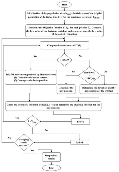
Figure 2.
Flow Chart of Optimal Smart meter placement through Jellyfish Optimization.
4. Graph Search Method to Divide Protection Zones
For the power system topology in this research, graph theory topologies such as Vertex (V) and Edges (E) are employed. These rules are detailed in reference [39]. The following rules are being examined for zone separation:
- Rule #1: If an original Bus is brought along through the present protection zone by a vertex, then a new protection zone will be formed.
- Rule #2: If the protection zone includes any identical buses, then one should maintain it and the other clone zones should be removed.
These two principles can be taken into account for the search issue, which is to find the ideally located smart meter in the protective zone. A unique protection strategy was presented based on the above two rules. The algorithm steps listed below have been examined on Transmission (IEEE 39 Bus) and distribution systems. The steps involved are shown in Figure 3.
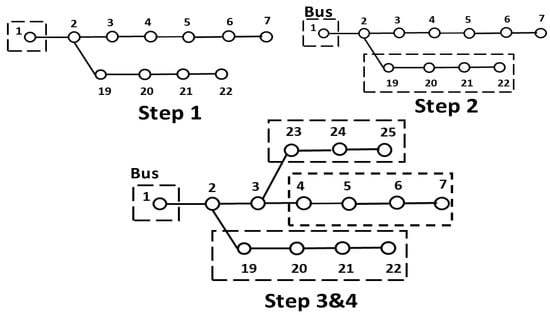
Figure 3.
Steps involved in the proposed Graph Search Method.
- Initial Step: every basic bus can be handled as an initial zone in the first stage. In the IEEE 39 test system, for example, bus 1 is a zone.
- Second Step: under this stage, the first bus seeks nearby buses and joins all of them to establish a new zone.
- Third Step: the search criteria in this phase in comparing the old zone to the latest zone generated in Step 2. If the zone contains any comparable buses, then this zone will be removed to ensure that all buses are protected consistently.
- Fourth Step: in this stage, the search algorithm determines whether the total number of buses in the zone equals the total number of buses in the network, and then it concludes the search procedure, or else, proceed to Step 2.
5. Steps of the Features Extraction Method
It is challenging to extract and improve the impact characteristics of the fault signals due to the system’s noise. To address this issue, we employ TQWT to dissect the fault signals into many scales, then extract the relevant sub-band to improve the signals’ impact characteristics. Here is the algorithm as follows:
- (a)
- Zone division: Select the measuring zone based on graph theory
- (b)
- Location of meters: Capturing voltage signal from optimized location based on JSO
- (c)
- The HHT is composed of two distinct components: the empirical mode decomposition (EMD) approach and the Hilbert transform. EMD is based on the decomposition of the initial signal x(t) into modal basis functions and the subsequent application of the Hilbert transform to these functions. These are known as intrinsic mode functions (IMFs). wavelet according to equation 22 calculates the PSK value to select the specific IMFs.
- (d)
- TQWT decomposition: optimal values for the TQWT parameters (Q, r, and J) and as per (18) SAEWSE has to be calculated. If SAEWSE is showing the lowest value then fixed the value of Q, r, and J.
- (e)
- Selection of decomposition layer: Based on (31) calculate the minimum value of MDL and find out the specific mother. If the MDL value is showing the lowest then consider that level as a perfect decomposition level for TQWT to make this method faster.
- (f)
- Feature extraction: As per (21) find out the polar plot which are the corresponding features of the faults.
- (g)
- Normalized entropy: According to (26) calculate the normalized entropy to distinguish between different types of faults.
- (h)
- SAEWSE calculation.
6. Results and Discussions
The suggested approach has been evaluated in IEEE 39 bus scheme shown in Figure 4. The details of the IEEE 39 bus scheme can be found in [38]. Figure 5 highlights the optimal location for the placement of the measuring devices with the application of JSO. The sampling time has been taken as 0.0997 ms, which resembles a 10.025 kHz sampling frequency. Thus, for the TQWT approach, 10.025 kHz has been fixed as the sampling frequency. In this proposed work, the sample size has been a vital parameter along with the sampling frequency. Here the number of samples is 2048 which is collected for 20 cycles.
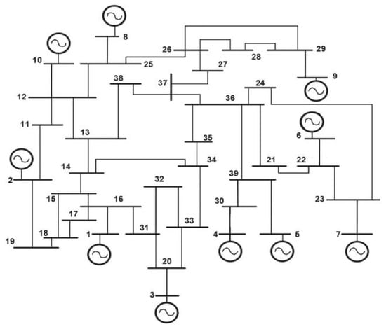
Figure 4.
IEEE 39 Bus scheme.
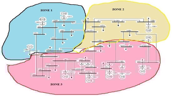
Figure 5.
Graph Theory-based Zone Selection.
To select the proper decomposition level and mother wavelet a proper algorithm has been chosen which is shown in Table 1 which is based on MDL. As per Table 1, level 3 with dB 10 is showing a minimum MDL value, i.e., −100.19. So, the fault voltage signal is decomposed up to level 3 to avoid the computational burden with a Q value is 3 and the r value is considered 3 which is shown in Figure 6a. After considering this value, level 3 is such a sub-band level where we found maximum energy distribution which can capture maximum fault-related information or features. The maximum sub-band frequency distribution is shown in Figure 6b. After j is determined, Q and r are selected to ensure that the fundamental and harmonic components are exactly extracted from the input signal, since the fundamental component with 50 Hz frequency is essential to select proper Q and r values for different PQ disturbance signals.

Table 1.
Choice of mother wavelet and decomposition level.
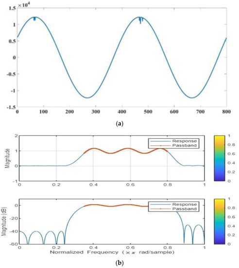
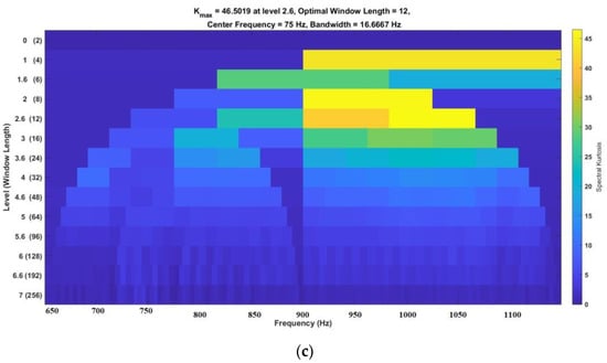
Figure 6.
(a) Simulated voltage signal for HIF (b) Selection of frequency band (c) Kourtogram for HIF.
6.1. Feature Extraction of HIF Fault
Mathematical domains that exhibit the HIF’s properties, such as its unpredictability, nonlinearity, nonstationary nature, and asymmetry, can be investigated via feature extraction. One should add a feature selection step to the design if the number of features derived from the analysis domain is significant, as this will raise the complexity of the classifier. Selecting the most informative features from a large feature set is the goal of feature selection.
The time domain waveform of the High Impedance fault is displayed in Figure 6. During this malfunction, there is a lot of noise in the signal, which pollutes the signal and dilutes the signature characteristics. The 3 dB bandwidth attenuation method [39] yielded the characteristic frequency band depicted in Figure 6b. The maximum value on the Magnitude vs. frequency curve corresponds to a driving frequency of 2048 Hz, while the upper and lower limits of the typical frequency band are indicated by the 3 dB bandwidth. It can be observed, the proposed optimal feature band selection approach is effective, as the major information of the signal can be contained within the region of 3 dB bandwidth. TQWT decomposition layers chosen from the upper and lower boundaries of the characteristic frequency band are depicted in a schematic form in Figure 6b.
In particular, the purpose of this research is to present a method for detecting the HIF that is based on a joint application of ensemble empirical mode decomposition (EEMD) and tunable Q factor wavelet transform (TQWT). First, the EEMD is applied to the signal in concern so that the voltage signal can be broken down into its intrinsic mode functions (IMFs). Then, the third IMF is selected as the highest PSK value. In this application IMF 3 has got the highest PSK value as per Figure 7 that shows the PSK value of each characteristic sub-band.
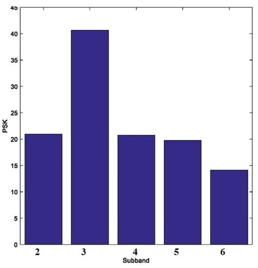
Figure 7.
Result of optimal characteristic sub-band selection.
Figure 8a,b depict the waveform and envelope spectra of the characteristic sub-band signal retrieved using wavelet packet decomposition and Ensemble empirical mode decomposition (EEMD) [39] decomposition, respectively, in the time domain based on (16). Three IMFs were created using the EEMD technique, and the ideal characteristic of the sub-band for IMF3 was calculated using the same maximum PSK value according to (22). As can be seen in Figure 8, the EEMD technique uses random noise to lower the amount of mode aliasing during the decomposition of the signal. Applying the M-point discrete Fourier transform (DFT) to Ey(j, n), we obtain the frequency domain sequence FE(j, ω), and then we calculate the power spectrum PE(j, ω) of the signal envelope of layer j where j = 3. As per the PSK value level, 3 can capture most of the information so signature features can be plotted as per (22). Moreover, the frequency and its frequency harmonic components of 1–5 that make up the impact characteristic are easily identified, demonstrating that the suggested method can extract the impact characteristic even when dealing with high levels of background noise.
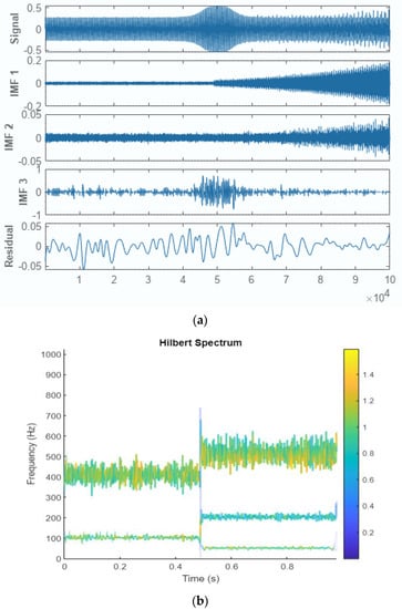
Figure 8.
(a) Ensemble Empirical mode decomposition (EEMD) of HIF signal (b) Hilbert transform of IMF 3.
The upper and lower frequency limit of the typical frequency band establishes the number of TQWT decomposition layers as shown by the Koutogram which is shown in Figure 6c. The kurtosis of the power spectrum is then used to identify the best possible characteristic sub-band The number of decomposition layers and mother wavelet has been selected as per Table 1.
When Q = 1 and r = 3, as shown in Figure 9 that depicts the SAEWSE value in the two-dimensional grid search space of parameter (Q,r); the ideal parameter (Qopt = 1, ropt = 3) is found based on the minimal SAEWSE curve value and the value of SAEWAE is the lowest. So these values are selected in this method. The parameters Q, r, and J were chosen based on their ability to maximize the weighted wavelet Shannon entropy of the sub-band average energy according to (18). The results of different decomposition layers are displayed in Figure 10. Based on the optimal parameters Q = 1 and r = 3, the simulation signal is broken up into four layers.
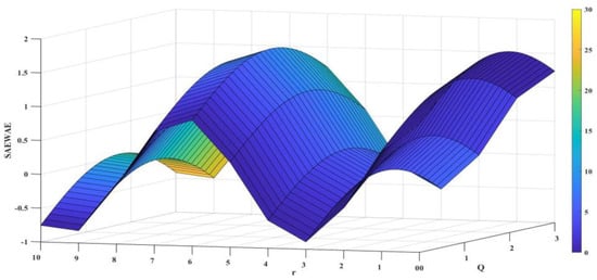
Figure 9.
3D curve of optimizing adaptive parameters for HIF.
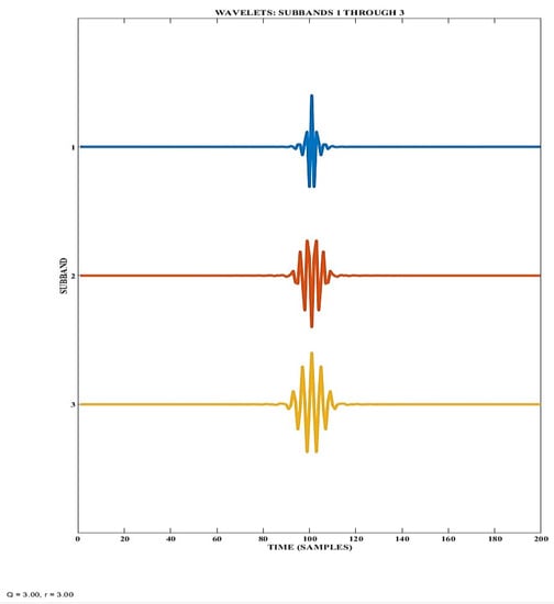
Figure 10.
3 layers TQWT decomposition.
6.2. Feature Extraction of CCHIF Fault
Based on Figure 11 three IMFs were created using the EEMD technique, and the ideal characteristic sub-band for IMF3 was calculated using the same maximum PSK value according to (22). After applying (22) the PSK value is showing highest at level 3 which is shown in Figure 12 that shows the PSK value of each characteristic sub-band.
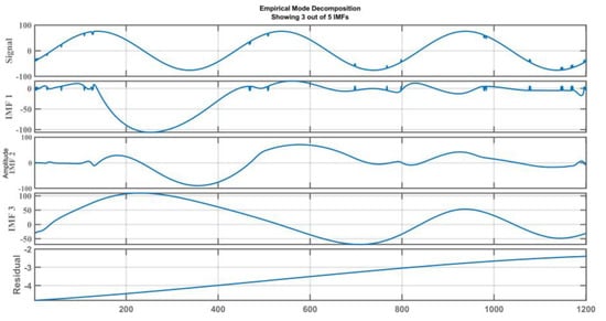
Figure 11.
3 layers of decomposition.
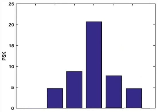
Figure 12.
Result of optimal characteristic sub-band selection.
Figure 13 is the frequency and its harmonic components of 1–5 that make up the impact characteristic are easy to find. This shows that the suggested method can extract the impact characteristic even when there is a lot of background noise. Figure 14 presents the results of applying TQWT to the faulted signal to perform decomposition (d–f). Figure 15 depicts the SAEWSE value in the two-dimensional grid search space of parameter (Q,r); the ideal parameter (Qopt = 1, ropt = 3) is found based on the minimal SAEWSE curve value. It displays the minimum SAEWSE value, which identifies the best parameter with which to decompose the recorded signal, as Q = 1 and r = 3.
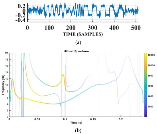
Figure 13.
(a) generated CCHIF voltage waveform, (b) Hilbert Spectrum of CCHIF waveform.
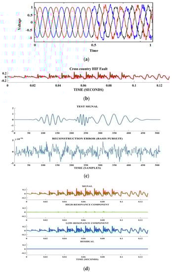
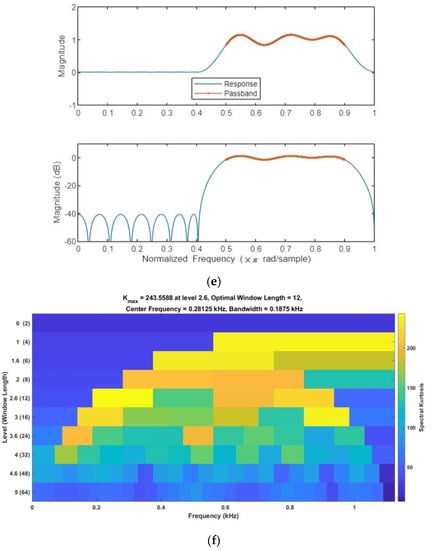
Figure 14.
(a) Three phase CCHIF signal (b) zoom view CCHIF single phase signal (c) reconstructed signal (d) decomposed signal (e) 3 dB bandwidth (f) Kurtogram of CCHIF.
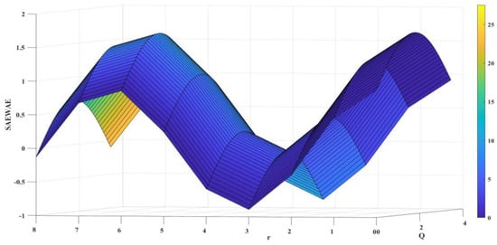
Figure 15.
3D curve of optimizing adaptive parameters for CCHIF.
Figure 14 shows the CCHIF fault time domain waveform. During this malfunction, the signal is polluted and diluted by noise. Figure 14 shows the characteristic frequency spectrum from 3 dB bandwidth attenuation (e). The 3 dB bandwidth indicates the upper and lower bounds of the usual frequency band, which is 2048 Hz on the Magnitude vs. frequency curve. The optimal feature band selection strategy works because the pulse’s main information fits inside the 3 dB bandwidth. This figure shows schematic TQWT decomposition layers from the upper and lower characteristic frequency band borders (b) MDL determined the number of decomposition layers to speed up this approach. The Koutogram in Figure 14 shows the number of TQWT decomposition layers based on the typical frequency band’s upper and lower limits (c). The power spectrum kurtosis determines the best characteristic sub-band. SAEWAE is lowest when Q = 1 and r = 3 (Figure 15). This method selects Q and r values for the TQWT application.
To extract the impact characteristics of the CCHIF fault, the proposed approach based on TQWT has been applied to extract the fault features. Based on the calculated parameters of TQWT parameters (Q = 1 and r = 3) features have been extracted. The factor redundancy r is the overall number of wavelet factors split by the length of the input signal to which the TQWT is employed [37]. As here the number of coefficients is 6144 and the length of the signal or number of samples is 2048 so here r = 3. The width of the bandpass filter is related to the Q-factor. The bandpass filter is significantly wide for low Q-factor, and few levels are needed for covering the spectral content of the signal of interest. The narrow bandpass filter is associated with a high Q-factor, and hence more levels are necessary for covering the spectrum of the signal. Hence in this method, Q = 1 has been chosen as the number of decomposition levels is 3. As per the filter specification in (6) and (7), μ = 0.666 and β = 0.778, hence the value of r = 3.
The entropy of each signal at every sub-band level is calculated. The optimal solution of the objective function is obtained as illustrated in (32–33) and the optimal solutions are also shown in Table 2. In Figure 6, a normal HIF fault is simulated in IEEE 39 bus system. In this figure voltage signal and sub-band energy, distribution has been shown to distinguish it from the CCHIF fault. The decision rules are made according to the values occurred by mean entropy values which are shown in Table 3 at every transient to identify and classify CCHIF from normal HIF fault and low impedance faults. In the second stage, a new zone protection scheme is proposed baes on the graph theory concept. This method divides a Transmission system into different zones to make protection easier and more efficient to handle the fault condition. As there are 6144 coefficients here and 2048 samples, r = 3. The Q-factor has something to do with how wide the bandpass filter is. The bandpass filter is very wide for having a low Q-factor, and it only needs a few levels to cover the signal’s spectral content. The high Q-factor of the narrow bandpass filter means that it needs more levels to cover the whole spectrum of the signal. Figure 6 shows that there are three levels of decomposition, so Q = 1 was chosen for this method. According to the filter requirements in (7) and (8), =0.666 and =0.778, so r = 3.
Table 2.
Optimal Placement of measuring devices.
Table 3.
Mean Entropy Values of Various Fault Circumstances.
The jellyfish search optimization technique is used to put the meters in the best place. The optimal solution of the objective function is shown in (51), and Table 2 also shows the optimal solutions for placing the metering devices.
To distinguish between CCHIF, HIF, and low impedance faults, the decision rules are based on the mean entropy values that are shown in Table 3 for each transient. In the second step, an idea from graph theory is used to come up with a new way to protect zones. This method divides a transmission system into different zones to make fault condition protection easier and more effective.
6.3. Calculation of Normalized Entropy
Table 3 represents the different mean or normalized entropy values based on [ for different power quality disturbances. In this paper, normalized values have been chosen to apply in all distribution networks. After rigorous experiments, it has been decided that these normalized entropy values are fixed for every distribution system, so these values are taken as significant values to differentiate between CCHIF and Non-CCHIF.
Decision rules are made according to the results that occurred from Table 3. According to these decision rules, entropy values falling below 0.2 are healthier signals, and values between 0.2 and 0.5 are categorized as high-impedance faults. The entropy values, which are above 0.5, are categorized as Low impedance Faults. CCF-HIFs are classified as high-impedance ground faults taking place in different phases of the individual circuit at several places at the same time as the fault initiation time. So, in this case, voltage and voltage waveform becomes more distorted. So, in this type of fault entropy value is showing higher than the normal HIF fault. As in this method we have considered normalized entropy, hence these values can be applied to any transmission lines.
Fault-diagnosis methods that rely heavily on data typically involve summarizing a large number of process variables into diagnostic sequences with fewer dimensions. The initial time series is expanded into empirical modal functions, and the Hilbert transform is applied to these functions [41] so that the instantaneous amplitudes and frequencies may be calculated at each instant in time. In addition, the TQWT coefficients that were acquired at level 3 and the instantaneous amplitudes are utilized for the automatic identification of ideal combinations of the variables that are used in the process of polar feature extraction. The polar plot representation method creates important measurements that may be used to determine which process variables contribute to fault conditions, and TQWT feature extraction enables process monitoring in feature and residual spaces. Figure 16a,b polar plot depiction of the features that were retrieved from the power system faults.
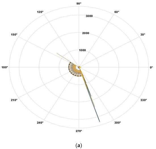
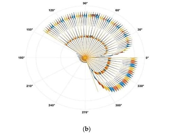
Figure 16.
(a) Polar representation of extracted features of HIF fault (b) Polar representation of extracted features of CCHIF fault.
6.4. The Effect Brought by the Changing of the Reactor String
In this section, the suggested fault diagnosis strategy is put through its paces under a variety of operating and switching conditions. This is accomplished through the switching function of reactor strings, such as line reactors. In IEEE 39 bus system, 50 MVA reactor strings were connected and CCHIF has created to determine the fault feature. In Figure 12 distorted voltage signal and extracted features are shown. Figure 17, which shows the frequency response of the TQWT band-pass filter, shows that three decomposition layers make the most sense.
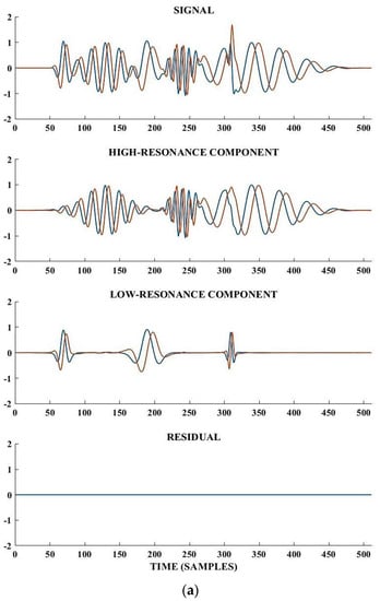
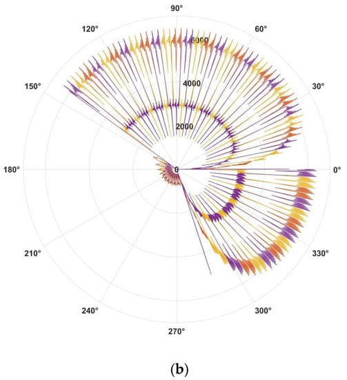
Figure 17.
(a) Voltage signal during reactor Charging (b) Extracted features.
The factor redundancy r is the total number of wavelet factors divided by the length of the signal that the TQWT is used on [37]. As there are 6144 coefficients here and 2048 samples, r = 3. The Q-factor has something to do with how wide the bandpass filter is. The bandpass filter is very wide for having a low Q-factor, and it only needs a few levels to cover the signal’s spectral content. The high Q-factor of the narrow bandpass filter means that it needs more levels to cover the whole spectrum of the signal.
The jellyfish search optimization technique is used to put the meters in the best place. It is used to figure out the entropy of each signal at each sub-band level. The optimal solution of the objective function is shown in (27), and Table 2 also shows the optimal solutions.
To determine the difference between CCHIF and low impedance faults, the decision rules are based on the mean entropy values that are shown in Table 3 for each transient. In the second step, an idea from graph theory is used to come up with a new way to protect zones. This method divides a transmission system into different zones to make fault condition protection easier and more effective. Figure 17a,b show the Voltage signal during reactor Charging and Extracted features, respectively.
6.5. Ferranti Effect
We must avoid the Ferranti effect when the load is relatively light or when the line is being energized. Transients can be caused by the switching of line reactors through de-energization and energization. These transients have the same appearance as transients caused by HIF syndrome. In this scenario, the switching operation of a three-phase line reactor with a 50 MVA rating is carried out, and then it is immediately followed by a faulty issue such as CCF-HIF to evaluate the discrimination capabilities of the presented topology while HIF syndrome is present. The transients that were created at LDCs by HIF syndrome. In this situation, the performance of the suggested fault identification technique was evaluated since the voltage, voltage, and temperature were all stable. In this case, also same extracted feature is the same which is shown in Figure 18.
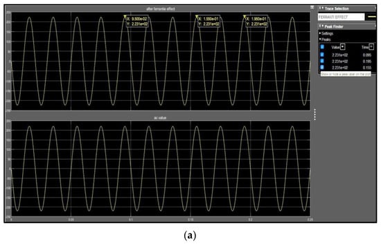
Figure 18.
(a) Simulated Ferranti Effect (b) Zoom view of the captured signal during CCHIF along with Ferranti effect.
6.6. Comparative Assessment
Several methods for locating cross-country HIF have previously been covered in Section 1. Other approaches found in the literature have been compared to the suggested method. The authors have taken into account scenarios of transient switching at various sampling frequencies together with various loading circumstances in the suggested technique (balanced and unbalanced). Using a real-time simulator, the performance of the suggested technique under dispersed generation and power electronic interfaced non-linear loads has been investigated.
For the suggested approach to identify cross-country HIF syndrome, a three-phase voltage signal is needed at any one monitored location. The suggested feature-extraction technique is very effective and simple for detecting this type of fault. It has a significant advantage in the detection of cross-country HIF syndrome in both quiet and noisy conditions. Additionally, TQWT-based techniques reduce the impact of uncorrelated random noise that is present in the signal, removing the need for extra caution to eliminate the impact of noise in the recorded signal. The TQWT-based method can identify HIF under a specific sampling frequency. Unbalanced load switching, dispersed generation, and power electronic interfaced non-linear loads. It is also highly effective at separating HIF from other transient conditions. Some alternative approaches are described in Table 4.
Table 4.
Comparative study.
7. Conclusions
The research offers a valid TQWT-based method for the recognition of cross-country HIF syndrome in the transmission network. The suggested method can effectively identify this exact feature of the CCHIF fault. The technique only analyses voltage signals at one monitoring point and in typical circumstances executes correlation operations with those voltage signals at that point. To obtain the faulty phase through cross-country HIF fault, only three features from the cross correlogram of voltage signals were used. The authors employed a TQWT-based method to reduce the computational burden by selecting proper decomposition levels. The TQWT-based approach also reduces the impact of random uncorrelated noise from the signal. To find the faulty bus, the authors have used the slime mould optimization technique to find the optimal locations in the network. This method is verified in different conditions such as reactor switching, load switching, and the Ferranti effect. In each case, this proposed method can be able to extract the features of the CCHIF fault.
To extract the impact characteristics of CCHIF Faults signals, an approach based on the adaptive TQWT method for parameter estimation is suggested. This method of selecting TQWT’s critical parameters is developed based on the time-frequency profile of the faulted signal. To further highlight the more impact components in the signal according to the feature frequency band, the optimization notion is included in the TQWT decomposition process, which greatly enhanced the capability to extract the transient characteristics of the signal.
Author Contributions
Conceptualization, P.S., K.P., A.Y.A., A.I.O., C.-L.S. and M.E.; Data curation, P.S., K.P. and C.S.; Formal analysis, A.Y.A., A.I.O., C.-L.S. and M.E.; Funding acquisition, C.-L.S. and M.E.; Methodology, P.S., K.P. and C.S.; Project administration, C.-L.S. and M.E.; Resources, P.S., K.P., A.Y.A. and C.S.; Software, P.S., K.P. and C.S.; Validation, P.S., K.P. and C.S.; Visualization, P.S., K.P. and C.S.; Writing—original draft, P.S., K.P. and C.S.; Writing—review & editing, A.Y.A., A.I.O., C.-L.S. and M.E. All authors have read and agreed to the published version of the manuscript.
Funding
The work of Chun-Lien Su was funded by the Ministry of Science and Technology of Taiwan under Grant MOST 110-2221-E- 992-044-MY3.
Data Availability Statement
The data presented in this study are available on request from the corresponding author. The data are not publicly available due to their large size.
Conflicts of Interest
The authors declare no conflict of interest.
References
- Jain, A.; Thoke, A.S.; Patel, R.N.; Koley, E. Inter-circuit and cross country fault detection and classification using artificial neural network. In Proceedings of the 2010 Annual IEEE India Conference (INDICON), Kolkata, India, 17–19 December 2010; pp. 1156–1161. [Google Scholar]
- Solak, K.; Rebizant, W. Analysis of differential protection response for cross-country faults in transmission lines. In Proceedings of the 2010 Modern Electric Power Systems, Wroclaw, Poland, 20–22 September 2010; pp. 1–4. [Google Scholar]
- Zin, A.M.; Omar, N.; Yusof, A.M.; Karim, S.A. Effect of 132kV Cross-Country Fault on Distance Protection System. In Proceedings of the 2012 Sixth Asia Modelling Symposium, Bali, Indonesia, 29–31 May 2012; pp. 167–172. [Google Scholar] [CrossRef]
- Xu, Z.Y.; Li, W.; Bi, T.S.; Xu, G.; Yang, Q.X. First-Zone Distance Relaying Algorithm of Parallel Transmission Lines for Cross-Country Nonearthed Faults. IEEE Trans. Power Deliv. 2011, 26, 2486–2494. [Google Scholar] [CrossRef]
- Bi, T.; Li, W.; Xu, Z.; Yang, Q. First-Zone Distance Relaying Algorithm of Parallel Transmission Lines for Cross-Country Grounded Faults. IEEE Trans. Power Deliv. 2012, 27, 2185–2192. [Google Scholar] [CrossRef]
- Swetapadma, A.; Yadav, A. Improved fault location algorithm for multi-location faults, transforming faults and shunt faults in TCSC compensated transmission line. IET Gener., Transmiss. Distrib. 2015, 9, 1597–1607. [Google Scholar] [CrossRef]
- Swetapadma, A.; Yadav, A. All shunt fault location including cross-country and evolving faults in transmission lines without fault type classification. Electr. Power Syst. Res. 2015, 123, 1–12. [Google Scholar] [CrossRef]
- Govar, S.A.; Sayedi, H. Adaptive CWT-based transmission line differential protection scheme considering cross-country faults and CT saturation. IET Gener. Transmiss. Distrib. 2016, 10, 2035–2041. [Google Scholar]
- Singh, S.; Vishwakarma, D. A Novel Methodology for Identifying Cross-Country Faults in Series-Compensated Double Circuit Transmission Lines. In Proceedings of the 6th International Conference Soft Computing Communication, Kurukshetra, India, 7–8 December 2017; pp. 7–8. [Google Scholar]
- Swetapadma, A.; Yadav, A. An artificial neural network based solution to locate the multi-location faults in double circuit series capacitor compensated transmission lines. Int. Trans. Elect. Energy Syst. 2018, 28, e2517. [Google Scholar] [CrossRef]
- Ashok, V.; Yadav, A. A Protection Scheme for Cross-Country Faults and Transforming Faults in Dual-Circuit Transmission Line Using Real-Time Digital Simulator: A Case Study of Chhattisgarh State Transmission Utility. Iran. J. Sci. Technol. Trans. Electr. Eng. 2019, 43, 941–967. [Google Scholar] [CrossRef]
- Ashok, V.; Yadav, A.; Abdelaziz, A.Y. MODWT-based fault detection and classification scheme for cross-country and evolving faults. Electr. Power Syst. Res. 2019, 175, 105897. [Google Scholar] [CrossRef]
- Kim, C.-H.; Kim, H.; Ko, Y.-H.; Byun, S.-H.; Aggarwal, R.; Johns, A. A novel fault-detection technique of high-impedance arcing faults in transmission lines using the wavelet transform. IEEE Trans. Power Deliv. 2002, 17, 921–929. [Google Scholar] [CrossRef]
- Nooshin, F.N.; Matinfar, H.R. Feature extraction of tree-related high impedance faults as source of electromagnetic interference around medium voltage power lines’ corridors. Prog. Electromagn. Res. B 2017, 75, 13–26. [Google Scholar]
- Maximov, S.; Torres, V.; Ruiz, H.F.; Guardado, J.L. Analytical Model for High Impedance Fault Analysis in Transmission Lines. Math. Probl. Eng. 2014, 2014, 837496. [Google Scholar] [CrossRef]
- Teklic, L.; Filipovic-Grcic, B.; Pavic, I.; Jercic, R. Detection of high impedance faults in power transmission network with non-linear loads using artificial neural network. In Proceedings of the International Colloquium on Lightning and Power Systems, Ljubljana, Slovenia, 18–20 September 2017; pp. 1–7. [Google Scholar]
- da Silva, J.; Costa, F.; Lira, G.; Santos, W.; Neves, W.; Souza, B.; Brito, N.; Paes, M. High impedance fault location—Case study with developed models from field experiments. In Proceedings of the 21st International Conference on Electricity Distribution, Frankfurt, Germany, 6–9 June 2011; pp. 1–4. [Google Scholar]
- Torres, V.; Maximov, S.; Ruiz, H.F.; Guardado, J.L. Distributed Parameters Model for High-impedance Fault Detection and Localization in Transmission Lines. Electr. Power Compon. Syst. 2013, 41, 1311–1333. [Google Scholar] [CrossRef]
- Ibrahim, D.K.; Eldin, E.S.T.; El-Zahab, E.E.-D.A.; Saleh, S.M. Unsynchronized fault-location scheme for non-linear HIF in transmission lines. IEEE Trans. Power Del. 2010, 25, 631–637. [Google Scholar] [CrossRef]
- Ibrahim, D.; Eldin, E.S.T.; Aboul-Zahab, E.M.; Saleh, S.M. Real time evaluation of DWT-based high impedance fault detection in EHV transmission. Electr. Power Syst. Res. 2010, 80, 907–914. [Google Scholar] [CrossRef]
- Musa, M.H.H.; He, Z.; Fu, L.; Deng, Y. A cumulative standard deviation sum based method for high resistance fault identification and classification in power transmission lines. Prot. Control Mod. Power Syst. 2018, 3, 30. [Google Scholar] [CrossRef]
- Kundu, M.; Debnath, S. High impedance fault classification in UPFC compensated double circuit transmission lines using differential power protection scheme. In Proceedings of the 2018 IEEE Applied Signal Processing Conference (ASPCON), Kolkata, India, 7–9 December 2018; pp. 54–58. [Google Scholar]
- Shah, J.; Desai, S.; Shaik, A.G. Detection and Classification of High Impedance Faults in Transmission Line Using Alienation-based Analysis on Voltage Signals. In Proceedings of the 2018 3rd International Conference for Convergence in Technology (I2CT), Pune, India, 6–8 April 2018; pp. 1–6. [Google Scholar] [CrossRef]
- Saleh, S.M.; Ibrahim, D.K. Non-linear high impedance earth faults locator for series compensated transmission lines. In Proceedings of the 2017 Nineteenth International Middle East Power Systems Conference (MEPCON), Cairo, Egypt, 19–21 December 2017; pp. 108–113. [Google Scholar] [CrossRef]
- Makwana, V.H.; Bhalja, B.R. A New Digital Distance Relaying Scheme for Compensation of High-Resistance Faults on Transmission Line. IEEE Trans. Power Deliv. 2012, 27, 2133–2140. [Google Scholar] [CrossRef]
- Hafidz, I.; Nofi, P.E.; Anggriawan, D.O.; Priyadi, A.; Purnomo, M.H. Neuro wavelet algorithm for detecting high impedance faults in extra high voltage transmission systems. In Proceedings of the in 2017 2nd International Conference Sustainable and Renewable Energy Engineering (ICSREE), Hiroshima, Japan, 10–12 May 2017; pp. 97–100. [Google Scholar]
- Patel, T.K.; Mohanty, S.K.; Chand, R. A comparative study of high impedance fault in transmission line using distance relay. In Proceedings of the 2017 4th International Conference on Advanced Computing and Communication Systems (ICACCS), Coimbatore, India, 6–7 January 2017; pp. 1–4. [Google Scholar] [CrossRef]
- Costa, F.B.; Souza, B.A.; Brito, N.S.D.; Silva, J.A.C.B.; Santos, W.C. Real-Time Detection of Transients Induced by High-Impedance Faults Based on the Boundary Wavelet Transform. IEEE Trans. Ind. Appl. 2015, 51, 5312–5323. [Google Scholar] [CrossRef]
- Mohammadnian, Y.; Amraee, T.; Soroudi, A. Fault detection in distribution networks in presence of distributed generations using a data mining–driven wavelet transform. IET Smart Grid 2019, 2, 163–171. [Google Scholar] [CrossRef]
- Ibrahim, M.A. Disturbance Analysis for Power Systems; Wiley-IEEE Press: Hoboken, NJ, USA, 2012; pp. 51–52. [Google Scholar]
- Thirumala, K.; Prasad, M.S.; Jain, T.; Umarikar, A.C. Tunable-Q Wavelet Transform and Dual Multiclass SVM for Online Automatic Detection of Power Quality Disturbances. IEEE Trans. Smart Grid 2016, 9, 3018–3028. [Google Scholar] [CrossRef]
- Shi, J.; Huang, W.; Shen, C.; Jiang, X.; Zhu, Z. Dual-Guidance-Based Optimal Resonant Frequency Band Selection and Multiple Ridge Path Identification for Bearing Fault Diagnosis Under Time-Varying Speeds. IEEE Access 2019, 7, 144995–145012. [Google Scholar] [CrossRef]
- Guo, H.; Zhang, D.; Liu, L.; Xing, B. Train Axle Bearing Fault Diagnosis Based on Tunable Q-factor Wavelet Transform. In Proceedings of the 2021 Global Reliability and Prognostics and Health Management (PHM-Nanjing), Nanjing, China, 15–17 October 2021; pp. 1–7. [Google Scholar]
- Zhang, X.; Ma, R.; Li, M.; Li, X.; Yang, Z.; Yan, R.; Chen, X. Feature Enhancement Based on Regular Sparse Model for Planetary Gearbox Fault Diagnosis. IEEE Trans. Instrum. Meas. 2022, 71, 3514316. [Google Scholar] [CrossRef]
- Jamode, H.; Thirumala, K.; Jain, T.; Umarikar, A.C. Knowledge-based Neural Network for Classification of Power Quality Disturbances. In Proceedings of the 2020 19th International Conference on Harmonics and Quality of Power (ICHQP), Dubai, United Arab Emirates, 6–7 July 2020; pp. 1–5. [Google Scholar]
- Jalil, M.; Samet, H.; Ghanbari, T.; Tajdinian, M. An Enhanced Cassie–Mayr-Based Approach for DC Series Arc Modeling in PV Systems. IEEE Trans. Instrum. Meas. 2021, 70, 9005710. [Google Scholar] [CrossRef]
- Gautam, S.; Brahma, S.M. Detection of High Impedance Fault in Power Distribution Systems Using Mathematical Morphology. IEEE Trans. Power Syst. 2012, 28, 1226–1234. [Google Scholar] [CrossRef]
- Liu, X.; Sun, A.; Hu, J. Transient feature extraction method based on adaptive TQWT sparse optimization. EURASIP J. Wirel. Commun. Netw. 2021, 2021, 111. [Google Scholar] [CrossRef]
- Abdelaziz, A.; Ibrahim, A.; Mansour, M.; Talaat, H. Modern approaches for protection of series compensated transmission lines. Electr. Power Syst. Res. 2005, 75, 85–98. [Google Scholar] [CrossRef]
- Saxena, D.; Bhaumik, S.; Singh, S.N. Identification of Multiple Harmonic Sources in Power System Using Optimally Placed Voltage Measurement Devices. IEEE Trans. Ind. Electron. 2014, 61, 2483–2492. [Google Scholar] [CrossRef]
- Kurbatskii, V.G.; Sidorov, D.N.; Spiryaev, V.A.; Tomin, N.V. On the neural network approach for forecasting of nonstationary time series on the basis of the Hilbert-Huang transform. Autom. Remote Control 2011, 72, 1405–1414. [Google Scholar] [CrossRef]
Disclaimer/Publisher’s Note: The statements, opinions and data contained in all publications are solely those of the individual author(s) and contributor(s) and not of MDPI and/or the editor(s). MDPI and/or the editor(s) disclaim responsibility for any injury to people or property resulting from any ideas, methods, instructions or products referred to in the content. |
© 2023 by the authors. Licensee MDPI, Basel, Switzerland. This article is an open access article distributed under the terms and conditions of the Creative Commons Attribution (CC BY) license (https://creativecommons.org/licenses/by/4.0/).