Transition to Multicellularity and Peto Paradox

Abstract

This paper aims to explain the transition to multicellularity as a consequence of the evolutionary response to stress. The proposed model is composed of three parts. The first part details stochastic biochemical kinetics within a reactor (potentially compartmentalized), where kinetic rates are influenced by random stress parameters, such as temperature, toxins, oxidants, etc. The second part of the model is a feedback mechanism governed by a genetic regulation network (GRN). The third component involves stochastic dynamics that describe the evolution of this network. We assume that the organism remains viable as long as the concentrations of certain key reagents are maintained within a defined range (the homeostasis domain). For this model, we calculate the probability estimate that the system will stay within the homeostasis domain under stress impacts. Under certain assumptions, we show that a GRN expansion increases the viability probability in a very sharp manner. It is shown that multicellular organisms increase their viability due to compartment organization and stem cell activity. By the viability probability estimates, an explanation of the Peto paradox is proposed: why large organisms are stable with respect to cancer attacks.

1. Introduction

In this paper, we focus on three enigmatic problems of biology: (I) why multicellular organisms emerge; (II) why complex multicellular organisms can be constructed with a relatively small number of genes, and (III) the Peto paradox on cancer and lifespan, i.e., why they are stable with respect to cancer attacks.

The origin of multicellular organisms presents a significant challenge for biological evolution theory. For instance, E. Koonin notes “The emergence and evolution of complexity at the levels of the genotype and the phenotype, and the relationship between the two, is a central (if not the central) problem in biology. Even leaving aside for now the problem of the actual origin of the very substantial complexity associated with the cellular level of organization, one cannot help wondering why the evolution of life did not stop at the stage of the simplest autotrophic prokaryotes, with 1000 to 1500 genes. Why instead did evolution continue, to produce complex prokaryotes possessing more than 10,000 genes and, far more strikingly, eukaryotes, with their huge, elaborately regulated genomes; multiple tissue types; and even ability to develop mathematical theories of evolution?” (see [1], Ch. 8, p. 250). Some approaches to the evolution of multicellularity were proposed in ([2,3]), describing this evolution as a result of an interaction between hosts and parasites. The emergence of multicellular organisms can be considered as a major evolutionary transition [4].

The second enigma is connected to several protein-coding genes. In fact, the human genome comprises approximately 22,000 protein-coding genes, a number that is comparable to the genomes of fruit flies and nematodes. Surprisingly, more complex multicellular organisms do not necessitate a higher number of genes, despite having a greater number of phenotypic traits and the need to adapt to numerous environmental constraints. These facts challenge the classical ideas of modern evolutionary synthesis. According to the celebrated Fisher geometric model, it can be demonstrated that the likelihood of improving fitness through random mutations diminishes as the organism’s complexity increases ([5]). Building upon Fisher’s approach, Orr estimated the adaptation rate $R_e=\frac{dlogF}{dt}$ as a function of the number of environmental constraints M, with F representing the average population fitness ([6], 2000, [7], 2005). Orr’s findings reveal that the adaptation rate becomes exponentially small when $M\gg 1$, a phenomenon known as the complexity cost or complexity barrier. Therefore, for large values of M, the complexity barrier becomes exponentially large.

Richard Peto was the first to notice that the cancer incidence does not correlate with the number of organism cells [8]. The cancer incidence in humans is much higher than the incidence of cancer in whales, despite whales having more cells than humans. For simplicity, suppose that the probabilities of cancer driver mutations are constant for all cells. Then whales should die from cancer more often than people and at an early age. In reality, they live for hundreds of years. No statistically significant relationship has been found between body size and cancer incidence, supporting Peto’s observation. This problem III is connected to I and II. In fact, the existence of multicellular organisms requires the suppression of cancer [9]. There exists a connection between the origins of multicellularity and cancer [10,11]. In order to build larger bodies, organisms must suppress cancer. According to ([12]), large organisms have more anticancer genes.

Let us outline the proposed model, which aims to address problems I–III. The first part describes stochastic biochemical kinetics within a reactor (potentially compartmentalized), where kinetic rates are influenced by random stress parameters such as temperature, toxins, oxidants, etc. The second part of the model is a feedback mechanism governed by a genetic regulation network (GRN). The third component is stochastic dynamics, which describe the evolution of this network. We assume that an organism remains viable as long as the concentrations of certain key reagents are maintained within a defined range (the homeostasis domain).

To describe GRNs that control responses to stress, radial basis function networks (RBFNs) are used. The inputs to these networks are the stress parameter values and the states of the system. By external stress, we mean any deviation in environmental parameters that could potentially harm the organism (whether multicellular or a single cell). The GRN produces an output dependent on its architecture and, ultimately, on the genetic code, s, which determines the architecture and interconnections within the GRN. Following [13], we assume that the GRN output and stress impact neutralize each other. Connections between units in these networks depend on coding sequences $s=(s_1,\dots ,s_N)$, $s_i\in \{0,1\}$ of Boolean genes. Such a stress response model is not new; however, herein, it uses a new key element connected to stem cell activity in the stress response. Multicellular organisms consist of many types of differentiated (somatic) cells, which form tissues, and stem cells. Stem cells can produce differentiated cells. In this paper, we provide mathematical justification for the well-known idea that cell differentiation emergence in evolution is a response to stress, particularly oxidative stress [14]. In different eukaryotic microorganisms, the induction of antioxidant mechanisms is associated with development. Note that stem cells are particularly susceptible to stresses ([15]) and they are regulated by stress. Experimental data show ([15]) that stem cell division provides tissue turnover and response to damage. Different stress factors induce stem cell division and differentiation. Many pathways that regulate stem cell functioning are also stress–response pathways [15]. So, stress is involved in the long-term maintenance of cell populations [15,16]. In this paper, to describe models for gene regulation in stem cells, we take into account experimental observations and ideas [14,15,16,17]. We propose that the biochemical response of multicellular organisms to stress is facilitated by different gene networks activated in various tissues. We imagine the entire organism as divided into compartments, with stem cell activity aiding in regulating each compartment’s response. Contemporary morphogenesis models explain the emergence of such compartments [18,19]. The model proposed can be considered to be a far-reaching extension of L. Valiant’s model of the ideal answer [20]. In Valiant’s model, organisms are viewed as Boolean circuits modeling responses to environmental stress through a GRN. Our proposed model builds upon this approach while also incorporating real biochemistry, the existence of compartments, and stem cell dynamics. We assume that an organism remains viable as long as the concentrations of certain key reagents are maintained within a specific domain (the homeostasis domain).

The results can be sketched as follows. For such a model, we determine the estimate of the probability that the system does not leave the homeostasis domain under the impact of stress. These estimates are given by Theorem 1 for models without compartments and stem cells and Theorem 2 for models with compartments and stem cells. Furthermore, it is shown that the RBF network growth makes biosystems stable for long time periods. We show that a state with a GRN of the maximal possible size is the most probable, with overwhelming probability. This indicates that evolution favors transitions to increasingly larger GRNs. Multicellular organisms exhibit higher viability compared to a simple colony of cells due to compartment organization and stem cell activity. By these results, we propose an explanation for Peto’s paradox. Moreover, we estimate the number of genes needed to encode GRNs supporting anti-stress responses.

1.1. Innovations

This article continues the series of works (see, for example, [21], 2006, [13], 2021), where the replicative stability concept is investigated. This concept is proposed by M. Gromov and A. Carbone [22]. It was shown that some properties of evolution could be explained by the need for biosystems to maintain homeostasis under the influence of stress and fluctuations (both internal and external), and this homeostasis support must be ensured through subsequent replications. Indeed, many aspects of evolution can be interpreted this way, for example, the tendency to increase the number of genes (see a review in ([23], 2014)). The key question, however, is to explain the complexity of genetic networks. An attempt to resolve this problem was made in ([13], 2021), where a model of the biochemical system’s response to stress was introduced. In this study, the entropy of a stressful environment is defined, and it is demonstrated that an effective response to stress is achievable if the binary logarithm of the size of the regulatory genetic network is at least as large as this entropy. Therefore, according to ([13], 2021), the main reason for the growth of regulatory networks involves the complexity and diversity of the stress environment.

In this paper, the main innovation, compared to previous works, is the use of a compartment model to describe a response to stresses. This model accounts for the modular structure of an organism and stem cell activity. The organism’s response to stress is mediated through cell populations in these compartments, with their dynamics governed by the standard Lotka–Volterra model. Such an approach allows us to address one of the key biological problems, the Peto paradox, because it will be shown that the organism size directly affects stress response mechanisms. The second innovation, with respect to ([13], 2021), is that we no longer need the complexity of the environment to explain the complexity of an organism’s genetic network. If the organism’s environment fluctuates, it is enough to initiate an increase in the complexity of the genetic network. The third intriguing innovative element is that when an organism is divided into compartments, there is no longer a need to fine-tune genetic regulatory networks (as in connectionist models [19]). Instead, it is enough to adjust an appropriate interaction between the compartments.

1.2. Organization of the Paper

The paper is organized as follows. Section 2 describes the different models. Furthermore, we outline the methods. In Section 4, we state the concept of viability under stochastic perturbations. The main results on viability (Theorems 1 and 2) can be found in Section 5. Furthermore, the proof of these results follows based on the standard estimates of the Ventsel–Freidlin theory ([24], 1984). By these viability estimates, in Section 7, we show that evolution has sufficient time to construct complex structures. In Section 8, we outline some contemporary morphogenesis models and explain why multicellular organisms can be encoded by a few genes. An explanation of Peto’s paradox is stated in Section 9. Discussions and conclusions can be found in the last section. Technical estimates are relegated in Appendix A.

2. Model

In this section, we describe the model. It unfolds in a few steps.

2.1. Chemical Kinetics with Random Stress Parameters

In this subsection, following ([13]), we consider systems of differential equations where the right-hand sides depend on a random process, $\xi \left(t\right)$. These systems read

$$\frac{dv}{dt}=f(v,\xi \left(t\right))t\ge 0,$$

(1)

where $v\left(t\right)={(v_1\left(t\right),\dots ,v_n\left(t\right))}^{\top }\in D$, where D is a compact domain in ${\mathbb{R}}^n$ with a smooth boundary $\partial D$, and $v_i\left(t\right)$ represent reagent concentrations. We assume that $f(v,\xi )={(f_1(v,\xi ),\dots ,f_n(v,\xi ))}^{\top }$ are sufficiently smooth functions of v; for example, multivariate polynomials in v and smooth functions of $\xi \in {\mathbb{R}}^p$. Functions $\xi \left(t\right)$ are trajectories of random processes, which are piecewise constant in t and take values in a compact subset ${\mathbb{D}}_E$ of ${\mathbb{R}}^p$, where the quantity $p\in \mathbb{N}$ is a dimension of the stress parameter $\xi$. These Markov processes $\xi \left(t\right)$ describe a random stress produced by an environment. For system (1), we set the following initial conditions:

$$v\left(0\right)=v^{\left(0\right)}.$$

(2)

Reaction terms, f, can be defined by the well-known models of chemical kinetics and population dynamics. The simplest choice from the law of mass action is

$$f_i(v,\xi )=\sum _{\mathbf{a}\in {\mathcal{R}}_i}{C}_{i,\mathbf{a}}\left(\xi \right)v_1^{a_1}{v}_2^{a_2}\dots v_n^{a_n},$$

(3)

where $\mathbf{a}=(a_1,\dots ,a_n)$ is a multi-index with integers $a_i\ge 0$, ${\mathcal{R}}_i$ are finite subsets of $I_n=\{1,\dots ,n\}$, and $C_{i,\mathbf{a}}$ denote coefficients that determine kinetic rates. One also uses rational nonlinearities, for example,

$$f_i(v,\xi )=\sum _{\mathbf{a}\in {\mathcal{R}}_i}{C}_{i,\mathbf{a}}\left(\xi \right)\frac{P_{i,\mathbf{a}}\left(v\right)}{Q_{i,\mathbf{a}}\left(v\right)},$$

(4)

where $P_{i,\mathbf{a}}\left(v\right)$ and $Q_{i,\mathbf{a}}\left(v\right)$ are polynomials. We suppose that $Q_{i,\mathbf{a}}\left(v\right)$ are separated from zero:

$$|Q_{i,\mathbf{a}}\left(v\right)|>{\delta }_0>0,$$

(5)

for all $i,\mathbf{a}$ and $v\in D$. Systems (1) with $f_i$ defined by (3) or (4) often occur in biochemistry and population dynamics.

To ensure the existence and uniqueness of solutions to the Cauchy problem (1), (2) for all $t\in [0,+\infty )$, we make the following assumption. Let

$$f(v,\xi )·n\left(v\right)\le 0\forall v\in \partial D\forall \xi \in {\mathbb{D}}_E$$

(6)

where $n\left(v\right)$ is a unit normal vector directed outside D at the point $v\in \partial D$. Then solutions to the Cauchy problem (1), (2) exist and are unique for all $t>0$.

Polynomial and rational functions $f_i$ may not fulfill conditions (6). Since our aim is to investigate the local stability of local equilibria, we consider narrow neighborhoods of those equilibria. Let $\overline{v}$ be the equilibrium under consideration. For $\delta >0$, we introduce a $\delta$-neighborhood of that equilibrium by

$$W_{\delta }=\{v:|v-\overline{v}|<\delta \},$$

(7)

where we assume that $W_{\delta }\subset D_H$, where $D_H$ is a viability (homeostasis) domain. We truncate nonlinearities in the $f_i\left(v\right)$ setting ${\tilde{f}}_i\left(v\right)=f_i\left(v\right)\chi \left(v\right)$, where $\chi \left(v\right)=0$ is defined as follows: $\chi \left(v\right)$ is a Heaviside-like function, which is equal to 0 outside of an open neighborhood $W_{\delta }$ of the equilibrium, and $\chi \left(v\right)$ is equal to 1 inside this neighborhood. Here, we assume that the neighborhood radius $\delta >0$ is so small that this neighborhood $W_{\delta }$ lies inside the homeostasis domain.

Moreover, let us note that an explicit form of $f_i$ is not essential in the subsequent statement; however, certain assumptions on the existence of the equilibria of system (1) and their stability should be fulfilled.

2.2. Extended Model with Anti-Stress Response Encoded by Genes

Different complicated models of gene regulation were proposed, for example, refs. [19,25] for Drosophila morphogenesis. Suppose reaction terms $f_i$ involve feedback, u:

$$f_i=f_i(v,\xi ,u),u=U_{net,s}(v,\eta ).$$

(8)

Here, $u=(u_1,u_2,\dots ,u_{n_{reg}})\in {\mathbb{U}}_R$, where

$${\mathbb{U}}_R=\{u\in {\mathbb{R}}^{n_{reg}},sup\left|u\right|<R\},$$

and $n_{reg}$ is a positive integer, $R>0$ is a constant. Here, the input $\eta$ is the averaged value of $\xi$ on an interval:

$$\eta \left(t\right)={\gamma }^{-1}{\int }_0^{t}exp\left(-\gamma (t-\tau )\right)\xi \left(\tau \right)d\tau ,$$

(9)

where $\gamma >0$ is a parameter. We are seeking regulators defined by a radial basis function network (RBFN):

$$U_{net,s}\in {\mathsf{\Phi }}_{N_{reg},\sigma }$$

(10)

where the function class ${\mathsf{\Phi }}_{N_{reg},\sigma }$ is defined in Appendix A.2.

We suppose that all parameters in $U_{net,s}$ are encoded by a Boolean genetic code s, where $s\left(t\right)=(s_1,\dots .,s_N)$ is a gene expression vector (see Appendix A.3). We have N Boolean genes $s_i\in \{0,1\}$; therefore, s are elements of the Boolean hypercube $S_N={\{0,1\}}^N$. The i-th gene may be switched on ($s_i=1$) or switched off ($s_i=0$). The strings, s, can depend on time: at certain time moments, they change as a result of mutations, gene drift, and other evolution forces.

2.3. Assumptions

Let us formulate natural assumptions to stress $\xi$, chemical kinetics, and the feedback.

Assumption 1. 

Assumption to ξ.

We suppose that ξ is the sum of a trend $\eta \left(t\right)$ and a small multiplicative noise:

$${\xi }_i\left(t\right)={\eta }_i\left(t\right)+\kappa \sum _{l=1}^{n_f}{h}_{il}(v,\eta \left(t\right))\frac{d{w}_l\left(t\right)}{dt},$$

(11)

where κ is a small positive parameter, $h_{il}$ are functions, and $w_l\left(t\right)$, where $l=1,\dots ,n_f$ are independent standard Wiener processes (therefore, $d{w}_l\left(t\right)/dt$ are white noises).

To describe the trend $\eta \left(t\right)$, we use the model of subsequent environmental shocks. We assume that $\eta \left(t\right)$ are piecewise constant functions. Let us denote ${\tau }_1,{\tau }_2,\dots ,{\tau }_k,\dots$ as an infinitely increasing sequence of time moments ${\tau }_j$. Let $\Delta \tau ={min}_j({\tau }_{j+1}-{\tau }_j)$. We suppose $\Delta \tau >>\Delta t_r$ and $\Delta \tau >>\Delta t_d$, where $\Delta t_r$ and $\Delta {\tau }_d$ are the average times of GRN reaction to stress and biochemical dynamics, respectively. At the ${\tau }_j$ moments, we have environment shocks, where an interaction between the environment and the biosystem changes. The assumptions on $\Delta \tau ,\Delta t_r$, and $\Delta t_d$ are natural. It means that changes in the organism’s environment are not very frequent and, therefore, organisms have time to react to them. Otherwise, it is difficult to expect that evolution could be successful.

Let us assume that, for $t\in [{\tau }_j,{\tau }_{j+1})$, the parameter $\eta \left(t\right)={\eta }^{\left(j\right)}$, where at each step j ${\eta }^{\left(j\right)}$ is chosen randomly. More precisely, at each interval $[{\tau }_k,{\tau }_{k+1}]$, the value $\eta$ is a constant random vector, which is distributed according to a continuous density probability function (pdf) $d\mu \left(\eta \right)$ with a support, which has a support in a compact, non-empty domain ${\mathbb{D}}_E\subset {\mathbb{R}}^p$.

Let us denote by ${\mathbb{R}}_{\delta }=\{\lambda \in \mathbb{C}:\lambda <-\delta \}$ the open half-planes of the complex plane $\mathbb{C}$.

Assumption 2. 

Equilibrium existence and stability.

We assume that for each $\eta \in {\mathbb{D}}_E$ and each $u\in \mathbb{U}$, the system

$$\frac{dv}{dt}=f(v,\eta ,u)t\ge 0$$

(12)

has a hyperbolic rest point $\overline{v}$, smoothly depending on η and u. This means the following: One has

$$f(\overline{v}(\eta ,u),\eta ,u)=0.$$

(13)

Consider the corresponding linearized operator $\mathbf{A}(\eta ,u)$:

$$\mathbf{A}(\eta ,u)=f_v^{\prime }(\overline{v}(\eta ,u),\eta ,u).$$

(14)

The operator $\mathbf{A}$ is uniformly hyperbolic and stable: there is a ${\delta }_{*}>0$, such that

$$Spe{c}_{\mathbf{A}(\eta ,u)}\subset {\mathbb{R}}_{{\delta }_{*}}\forall u\in \mathbb{U},\eta \in {\mathbb{D}}_E.$$

(15)

This means that the biochemical equilibrium is uniformly stable in $(\eta ,u)$.

To formulate the next assumption, let us introduce important auxiliary functions. Let us define $g_{il}(v,\eta ,u)$ by

$$g_{il}=\sum _{j=1}^p\frac{\partial f_i}{\partial {\xi }_j}(v,\eta ,u)\sum _{l=1}^{n_f}{h}_{jl}(v,\eta ).$$

(16)

where $i=1,2,\dots ,n$ and $l=1,2,\dots ,n_f$, where $n_f$ is a positive integer, and $h_{jl}$ are smooth functions.

Assumption 3. 

Existence of an ideal feedback

We suppose for each $\eta \in {\mathbb{D}}_E$ and $v\in D_H$, there exists a solution $u=U^{*}(v,\eta )$ of the system

$$g_{il}(v,\eta ,u)=0,i=1,\dots ,n,l=1,\dots ,n_f,$$

(17)

which is a smooth function defined on the domain $D_H\times {\mathbb{D}}_E$.

This assumption means that there is an ideal response to the stress impact $\eta$. The GRNs should approximate this response to support the organism’s viability, as described in the last assumption.

Assumption 4. 

We suppose that for sufficiently large sizes, N, the ideal feedback $u=U^{*}(v,\eta )$ (which exists according to Assumption 3) can be approximated with a polynomial accuracy:

$$\underset{v\in D_H,\eta \in {\mathbb{D}}_E}{sup}|U^{*}(v,\eta )-U_{net}(v,\eta )|<{\overline{C}}_0{N}^{-\gamma }$$

(18)

by a network $U_{net}\in {\mathsf{\Phi }}_{N,\sigma }$, where constants ${\overline{C}}_0,\gamma >0$ are uniform in N.

This assumption can be justified by estimates stated in Appendix A.2. Moreover, Assumptions 3 and 4 show that our model can be considered an extension of L. Valiant’s circuit model of the ideal answer ([20], 2006, [26], 2009), where we take into account the biochemical kinetics, compartment existence, and the cell dynamics (which will be described below).

2.4. Stochastic Equations for Perturbations Induced by Stress Fluctuations

Taking into account our assumptions on $\xi$ and the existence of the equilibrium, we represent v as

$$v=\overline{v}(\eta ,u)+\tilde{v}\left(t\right)$$

where $\tilde{v}$ is a new unknown function, representing a small correction to the equilibrium. By Assumption 2, one has

$$f_i(v,\xi ,u)=f_i(v,\xi ,u)-f_i(\overline{v},\eta ,u)=P_i(v,\xi ,u)+R_i(v,\xi ,u),$$

(19)

where

$$P_i=f_i(v,\eta ,u)-f_i(\overline{v},\eta ,u),R_i=f_i(v,\xi ,u)-f_i(v,\eta ,u).$$

Using the Taylor expansion of f and the definition (14) of the linear operator $\mathbf{A}$, we obtain

$$P_i={\left(\mathbf{A}\tilde{v}\right)}_i+h_i(\tilde{v},\xi ,u),$$

where

$$|h_i\left(\tilde{v}\right)|<C|\tilde{v}{|}^2.$$

(20)

One has the following formal asymptotics for $R_i$:

$$R_i=\kappa {f_i}_{\eta }^{\prime }(\eta ,u)\xi +O\left({\kappa }^2\right).$$

(21)

Using (11), one finds that

$$R_i=\kappa \sum _{j=1}^p\frac{\partial f_i}{\partial {\eta }_j}\sum _{l=1}^{n_f}{h}_{jl}(v,\eta )\frac{d{w}_l\left(t\right)}{dt}+O\left({\kappa }^2\right).$$

(22)

We remove the terms $O\left({\kappa }^2\right)$ in $R_i$ and substitute the obtained shorted $R_i$ into (19), then one has

$$f_i(v,\xi ,u)={\left(\mathbf{A}\tilde{v}\right)}_i+h_i(\tilde{v},\xi ,u)+\kappa g_{il}(v,\eta ,u)\frac{d{w}_l\left(t\right)}{dt},$$

where $g_{il}$ is defined by (16).

Thus, for each time interval, where $\eta \left(t\right)$ does not change, we have the system of the following stochastic Ito equations

$$d{\tilde{v}}_i=\left({\left(\mathbf{A}\tilde{v}\right)}_i+h_i(\tilde{v},u)\right)dt+\kappa \sum _{l=1}^p{g}_{il}(v,\eta ,u)d{w}_l,$$

(23)

where $w_l$ are independent standard Wiener processes. We suppose that in these equations, u is defined by (8). Note that our derivation of these equations is only formal; for example, in (21), we remove the terms proportional to ${\kappa }^2$, which involve unbounded quantities ${(d{w}_l/dt)}^2$ (the Wiener processes are not smooth). This difficulty can be circumvented ([23], 2014). Nonetheless, we will use Equation (23) because it has a classical form of the Ito equations, which are well-studied and fundamental in applications; see [27].

2.5. Model with Compartments

In biology and medicine, compartment models are popular for biochemical applications, for example, to describe pharmacokinetics (see, for example, [28]). We consider a model consisting of $N_c$ compartments. Each compartment consists of differentiated cells of the k-th type, where $k=1,\dots ,N_c$, and $N_c$ is the number of cell types. Reaction terms in k-th compartments are denoted by $f_i^{\left(k\right)}$. Furthermore, each cell produces its own response to a stress disturbance $\eta$, which depends on the cell type. We denote by $U^{\left(k\right)}(v,\eta )$ the corresponding feedback (where we omit a dependence on the gene code s to simplify the notation). Let $X_k\left(t\right)$ be a relative abundance of cells of k-type, which produces an answer to stress. One can assume that the dynamics of these quantities are governed by the multispecies Lotka–Volterra dynamics with parameters depending on the stress parameter $\eta$:

$$\frac{d{X}_k}{dt}=X_k(r_k\left(\eta \right)-\sum _{l=1}^{N_c}{K}_{kl}\left(\eta \right)X_l),$$

(24)

where $r_k$ are growth-mortality coefficients, which take into account the apoptosis and production of differentiated cells by stem cells, and $K_{kl}$ denotes interaction coefficients. We have a dependence on $\eta$ because the behavior of stem cells depends on the stress factors (see Introduction and [14,15,16,17]). However, real organisms consist of cells; therefore, these variables, $X_k$, which are relative concentrations, take discrete values. For each positive integer, M, let us define the sets:

$$K_{+,M}=\{0,1/M,2/M,\dots ,m/M,\dots \}.$$

In a discrete model, we suppose that $X_k\in K_{+,N_{cell}}$, where $[1,n]$ denotes the set $\{1,2,\dots ,n\}$ and $N_{cell}$ is the total number of cells in the organism. To describe the dynamics, where cell abundances take discrete values, we can replace (24) with the stochastic Markov dynamics, which simulate system (24) by the Gillespie algorithm [29]. We suppose that the total anti-stress response of the whole organism is proportional to $X_k$ and $U^{\left(k\right)}$:

$$u(X,v,\eta )=\sum _{k=1}^{N_c}{X}_k{U}^{\left(k\right)}(v,\eta ).$$

(25)

The stochastic Equation (23) takes the form

$$d{\tilde{v}}_i=\left({\left(\mathbf{A}\tilde{v}\right)}_i+h_i(\tilde{v},u(X,\eta ))\right)dt+\kappa \sum _{l=1}^p{g}_{il}(\eta ,u(X,\eta ))d{w}_l,$$

(26)

where u is defined by (25).

Within the framework of this weakly nonlinear approximation, all information about the interaction (coupling–decoupling) of reactants is contained in matrix $\mathbf{A}$. We can define the coupling graph $(V,E)$, where the set V of vertices is the set of reactants, and an edge $e=i,j$ lies on the edge set E if the i-th reactant interacts with the j-th one. One can consider various cases of the interactions of reactants that are relevant from a biological point of view. For example, we can consider the case of a Michaelis–Menten reaction chain. In this case, the analysis of the spectrum of the operator specified by the matrix $\mathbf{A}$ is relatively simple. A more complex option involves several parallel reactions or parallel chains of Michaelis–Menten reactions. For systems with a large number of reactants, the case of random pairing (of a random E) is also interesting. A more detailed analysis of the coupling problem has been postponed for future work.

In the coming subsection, we describe how the population dynamics for $X_k\left(t\right)$ can produce an effective stress response.

2.6. Associated Optimization Problems

Let $u\left(\eta \right)$ be a smooth function defined on ${\mathbb{D}}_E$. When we try to approximate an ideal answer by GRNs acting independently in each compartment, we obtain the risk function $F_{risk}(X,\eta )$, defined by

$$F_{risk}(X,v,\eta )=\sum _{k=1}^{N_c}{|u(v,\eta )-X_k{U}^{\left(k\right)}(v,\eta )|}^2,$$

(27)

where $X={(X_1,\dots ,X_{N_c})}^{\top }$ is a vector with real-valued components and $\left|u\right|$ denotes the standard Euclidean norm in ${\mathbb{R}}^{n_{reg}}$. The approximation problem reduces to

Relaxed optimization problem RP To find X giving the minimum of $F_{risk}$ under conditions

$$X_k\ge 0,k=1,\dots ,N_c$$

(28)

and

Integer optimization problem IP To find X giving the minimum of $F_{risk}$ under conditions

$$X_k\in K_{+,N_{cell}}.$$

(29)

This last problem involves finding the anti-stress response via the correct activation of discrete cell sets.

First, consider the problem RP. If this problem has a solution, then that solution can be found by the population dynamics defined by system (24) under an appropriate choice of coefficients $K_{kl}$ and $r_l$. To show it, let us define a square matrix M of size $N_c\times N_c$ and the vector b:

$$M_{kl}=(U^{\left(k\right)}(v,\eta ),U^{\left(l\right)}(v,\eta )),k,l=1,\dots ,N_c,$$

(30)

$$b_k=(u(v,\eta ),U^{\left(k\right)}(v,\eta ))k=1,\dots ,N_c.$$

(31)

where $(,)$ is the Euclidean scalar product in ${\mathbb{R}}^{n_{reg}}$. Let us consider the Cauchy problem defined by the system of equations

$$\frac{d{X}_i}{dt}=-X_i\frac{\partial F_{risk}}{\partial X_i}$$

(32)

with $i\in [1,N_c]$ and positive initial conditions $X_k\left(0\right)=x_k>0$, where $x_k$ can be chosen at random. It is clear that this system can be rewritten in the form (24). System (32) enjoys the remarkable properties. First, the quantities $X_k\left(t\right)$ remain positive for all t; therefore, condition (28) holds. Furthermore, for fixed $v,\eta$, the function $L\left(X\right)=F_{risk}(X,v,\eta )$ is a Lyapunov function for system (32), decreasing along trajectories $X\left(t\right),t\ge 0$. In fact, Equation (32) implies

$$\sum _{l=1}^{N_c}{X}_l^{-1}{\frac{d{X}_l}{dt}}^2=-\sum _{l=1}^{N_c}\frac{\partial L}{\partial X_l}\frac{d{X}_l}{dt}=-\frac{dL}{dt}\le 0.$$

We observe that $F_{risk}\left(X\right)$ is a convex function of X defined on the convex domain, $D_X$. Therefore, the optimization problem RP has a unique solution. This solution can be found by system (32). Indeed, the Lyapunov function $L\left(X\right)$ is convex. Therefore, it has a single local minimum $X^{*}$. According to classical results on gradient-like dynamical systems, all the trajectories $X\left(t\right)$ converge to $X^{*}$ [30]. We note that the vector $X^{*}$ gives the solution to the optimization problem RP. Finally, we conclude that population dynamics give the solution to that optimization problem RP. We suppose that the domain, $D_X$, is convex, as we would like to deal with a convex optimization problem, where the global minimum is unique. To achieve this uniqueness property, not only must the objective function be convex, but the feasible set must be convex as well. In our biological context, the most natural choice for the domain is the simplex $X_k\ge 0$, ${\sum }_k{X}_k<C_x$, where $C_x>0$ is a constant.

A good approximation for solutions $X_I^{*}$ of the problem IP can be found for large $N_{cell}$, as follows: First we solve QP and obtain the solution $X^{*}$ (as described above). Then we make the standard relaxation procedure, replacing each $X_i^{*}$ with the corresponding closest element of the set $K_{+,N_{cell}}$. We denote an X obtained by $X_I^{*}$. We note that

$$|F_{risk}\left(X^{*}\right)-F_{risk}\left(X_I^{*}\right)|<C{N_{cell}}^{-1},$$

(33)

where C is a constant. If $F_{risk}\left(X^{*}\right)=0$ for certain feedback, $U^{\left(k\right)}(v,\eta )$, we have

$$F_{risk}\left(X_I^{*}\right)<C{N_{cell}}^{-1}.$$

(34)

Let us find sufficient conditions under which this estimate is satisfied. Note that the set

$${\mathbb{C}}_H(u^{\left(1\right)},\dots u^{\left(m\right)})=\{u\in {\mathbb{R}}^n:\sum _{k=1}^{N_c}{X}_k{u}^{\left(k\right)},X_k\ge 0,\sum _k{X}_k=1\}$$

is the simplex with vertices $u^{\left(k\right)}$. For each $v\in W_{\delta }$ let us consider the set ${\mathbb{U}}_v^{*}$ of all possible ideal answers

$${\mathbb{U}}_v^{*}=\{u\in {\mathbb{R}}^{n_{reg}}:\exists \eta \in {\mathbb{D}}_E,u=U^{*}(v,\eta )\}.$$

Proposition 1. 

Let $m\ge n_{reg}+1$. Assume that for each $v\in W_{\delta }$, one has the inclusion

$${\mathbb{U}}_v^{*}\subset {\mathbb{C}}_H(u^{\left(1\right)},\dots ,u^{\left(m\right)})$$

where $u^{\left(k\right)}\in {\mathsf{\Phi }}_{N,\sigma }$. Then for each $v\in W_{\delta }$, there is a $X^{*}\in {\mathbb{R}}^{N_c}$, such that $F_{risk}\left(X^{*}\right)=0$ and, thus, (34) holds.

Proof. 

It follows at once from the definitions. □

This claim indicates that adapting to stresses does not necessitate fine-tuning genetic networks within the differentiated cells of multicellular organisms. To create an effective response to stress, it is enough to correctly encode interactions between cells in different compartments. Moreover, the Carathéodory Theorem leads to the following conclusion: to satisfy (34), it is sufficient to have more cell types than the regulator dimension: $N_c>n_{reg}$.

2.7. Stochastic Equation for Feedback Evolution

In this subsection, we describe a model for the evolution of the GRN evolution. Let $U_{net,s}\left(\eta \right)$ be feedback maps, where all parameters are encoded by binary genes $s=(s_1,s_2,\dots ,s_N)$ (see Appendix A.3). At the initial moment, we have a random binary string $s\left(0\right)$. Consider the time interval $[0,T]$, where $T>>1$ is big. We choose a sequence of random moments $T_1,T_2,\dots ,T_m\in [0,T]$ such that $T_1<T_2<\dots <T_m<T$ Ȧt these moments, mutations occur in s. To describe this process, we can use an analog of the master equation basic in physics. Let $p(s,t)$ represent the probability that the system is in state s at time t. The probability of transitioning from s to $s^{\prime }$ is denoted by $w(s\to s^{\prime })$. We also introduce a special state corresponding to the destruction of the system, 0, and the probability of transitioning from s for 0 will be denoted by $q\left(s\right)$. We suppose that the likelihood of survival is completely determined by s (the theory of gene-trait maps, pioneered by R. Fisher ([5], 1930); see also [7,31,32]). Then we have

$$\frac{dp(s,t)}{dt}=\sum _{s^{\prime }}w(s^{\prime }\to s)p(s^{\prime },t)-\sum _{s^{\prime }}w(s\to s^{\prime })p(s,t)-q\left(s\right)p(s,t),$$

(35)

$$\frac{dp(0,t)}{dt}=\sum _{s}q\left(s\right)p(s,t).$$

(36)

To make this general model mathematically tractable, we simplify these equations as follows. Instead of the evolution of the genetic code, we consider an evolution in a space of GRN sizes, neglecting details of gene coding. The evolutionary step is conceptualized as an increase in the GRN size as a result of mutations (possibly, a few mutations are necessary).

We simplify the master equation as follows. Instead of the states s, we consider states defined by positive integers that define the network sizes, $m=N$, where $m\in \{N_0,\dots .N_{max}\}=[N_0,N_{max}]$ and $N_0>>1$. We consider the transitions $m\to m+1$ ahead only (the networks can extend and cannot shrink). For brevity, the corresponding transition probabilities are denoted by $w_m$. We obtain the following equations:

$$\frac{d{p}_m}{dt}=-(w_m+q_m)p_m+w_{m-1}{p}_{m-1},$$

(37)

where we suppose that $m\in [N_0,N_{max}]$, $w_{N_0-1}=0$, $w_{N_{max}}=0$, and $p_m$ is the probability of having a network of size m. These conditions mean that, in particular, the maximal network size is $N_{max}$. This equation can be written down in a short matrix form, as $dp/dt=\mathbf{W}p$, where $p={(p_1,\dots ,p_m)}^{\top }$, and $\mathbf{W}$ is the transition matrix for (37).

3. Materials and Methods

The classical methods of mathematical analysis and theory of differential equations are applied together with the results on approximations of smooth functions by RBF networks [33]. Our approach is based on the following:

(i) The idea of M. Gromov–A. Carbone on replicative stability in systems supporting homeostasis [22];

(ii) The theory of large deviations and stochastic transitions in random dynamical systems (A. Ventsel, M. Freidlin, Yu. Kifer et al.) ([24], 1984);

(iii) Models of morphogenesis proposed by A. Turing ([34]) and others ([19,35,36,37]);

(iv) Universal approximations by networks [33,38,39].

4. Stochastic Stability

Let us formulate the stochastic stability problem.

Following [13], we introduce probability, where for a given feedback $u=u\left(\eta \right)$, the solution $v(t,v^{\left(0\right)})$ of the Cauchy problem defined by (1) with initial data (2) lies in $W_{\delta }$ within the time interval $[0,\tau ]$:

$${\mathbb{P}}_{\delta ,\tau ,u}=Prob\{v(t,v^{\left(0\right)})\in W_{\delta }\forall t\in [0,\tau ]\}.$$

(38)

We suppose that the initial value is the equilibrium: $v^{\left(0\right)}=\overline{v}$. The probability ${\mathbb{P}}_{\delta ,\tau ,u}$ can be considered a measure of stochastic stability. A more relevant measure of stochastic robustness is given by the minimum over all network regulators, u:

$${\mathbb{P}}_{\delta ,\tau }=\underset{u\in {\mathsf{\Phi }}_{N,\sigma }}{inf}{\mathbb{P}}_{\delta ,\tau ,u},$$

(39)

where the infimum is taken over all feedback functions defined by RBFN of size N.

In the multi-compartment case, we take infimum over all $X_k$ and $U^{\left(k\right)}$:

$${\mathbb{P}}_{\delta ,\tau }=\underset{X_k\in K_{N_{cell}},U^{\left(k\right)}(v,\eta )\in {\mathsf{\Phi }}_{N,\sigma },k=1,\dots ,N_c}{inf}{\mathbb{P}}_{\delta ,\tau ,U^{*}(X,v,\eta )},$$

(40)

where

$$U^{*}(X,v,\eta )=\sum _{k=1}^{N_c}{X}_k{U}^{\left(k\right)}(v,\eta ).$$

5. Main Results

Let us formulate the main results. First, we choose $\delta >0$ in a special way. If it is necessary, we diminish $\delta$ to satisfy the following condition:

$$|(\mathbf{A}\tilde{v},\tilde{v})|>>||h\left(\tilde{v}\right)\left|\right|,\forall \left|\right|\tilde{v}\left|\right|<\delta .$$

(41)

Theorem 1. 

Let (41) hold. Consider the stochastic Equation (23) under Assumptions 1–4. Let the feedback $u=U_{net}(v,\eta )$ satisfy estimate (18).

Then one has the following estimate of the stochastic stability via the network size N, as $\kappa \to 0$:

$${\mathbb{P}}_{\delta ,\tau }=1-P_{out,\kappa ,N},$$

(42)

where

$${\kappa }^{2}log{P}_{out,\kappa ,N}<-C_{sur}{\delta }^2{N}^{2\gamma },$$

(43)

where $C_{sur}$ is a positive constant, depending on f, and uniform in $(\kappa ,N)$.

The second theorem concerns the multi-compartment case.

Theorem 2. 

Consider the multi-compartment system (26) under Assumptions 1–4. Let conditions of Proposition 1 hold. Then one has the following estimate of the stochastic stability via the numbers $N,N_{cell}$ as $\kappa \to 0$:

$${\mathbb{P}}_{\delta ,\mathcal{A},\tau }=1-P_{out,\kappa }$$

(44)

where

$${\kappa }^{2}log{P}_{out,\kappa }<-C_1{N}_{cell}^{-1}{\delta }^2,$$

(45)

where $C_1$ is a positive constant that is uniform in $\kappa >0$ and $N_{cell}$.

6. Proof of Theorems 1 and 2

Proof. 

Let us estimate the probability $P_{out,\kappa ,N}$ that the trajectory $v\left(t\right)$ exits $W_{\delta }$ within the time interval $[0,T]$ under the condition that $v\left(0\right)=\overline{v}$. We use the following estimate (see Appendix A.4) for the probability $P_{out}$:

$${\kappa }^{2}log{P}_{out,\kappa ,N}<-C\left(f\right){\delta }^2{\left|\right|g\left|\right|}^{-2},$$

(46)

where

$${\left|\right|g(v,\eta ,u)\left|\right|}^2=\underset{i}{max}\sum _{l=1}^p{\left|g_{il}(v,\eta ,u)\right|}^2.$$

Let us estimate $\left|\right|g(\overline{v},\eta )\left|\right|$, considering the size of the network N. According to Assumption 3, there exists a $U^{*}(v,\eta )$, such that

$$g_{il}(v,\eta ,U^{*})=0\forall i,l.$$

Due to (18)

$$\underset{i,l,\eta \in {\mathbb{D}}_E}{sup}|g_{il}\left(U^{*}(v,\eta )\right)-g_{il}{U}_{Net}(v,\eta )|<C_1{N}^{-\gamma },$$

thus

$$\underset{i,l,\eta \in {\mathbb{D}}_E}{sup}\left|g_{il}{U}_{Net}\left(\eta \right)\right|<C_2{N}^{-\gamma },$$

where $C_1,C_2>0$ are constants. This last estimate and (46) imply the assertion of Theorem. □

To prove Theorem 2, we repeat the same arguments in the proof of Theorem 1 and use definition of $F_{risk}$.

7. Transitions to Complex GRN

Using estimates of viability from Theorems 1 and 2 and the simplified Master Equation (37), we can estimate the probability of reaching the maximally complex regulation network state, $m=N_{max}$.

Let us denote by N the size of the gene network of the regulation. In real genetic networks, the degrees of the most nodes are bounded. Therefore, we need a bounded number $N_{mut}=O\left(1\right)$ of mutations, when the network increases its size from N to $N+1$ as a result of the gene code modification $s\to s^{\prime }$. It is natural, therefore, to assume that the transition probabilities $w_m$ admit the estimate:

$$w_m=w(m\to m+1)>C{p}_{mut}^{N_{mut}},N_{mut}<C_{*}$$

(47)

where $p_{mut}>0$ is a probability of a single mutation and a constant $C_{*}$ is uniform in the network size m. It is shown by Theorem 1 that

$$log{q}_m<-C{\kappa }^{-2}{m}^{2\gamma },\gamma >0,$$

(48)

where $C>0$ is uniform in m. Under these assumptions, the following claim holds:

Proposition 2. 

Let $w_m,q_m$ satisfy (47) and (48), respectively, and $p_{N_0}\left(0\right)=1$. Then for $N_0>>1$, sufficiently small $\kappa >0$ and t, such that $t>>{max}_{m\in [N_0,N_{max}]}{w_m}^{-1}$ one has that the solution $p\left(t\right)$ lies in the state $N_{max}$ with an overwhelming probability, as $N_0\to \infty$:

$$\underset{m\ne N_{max}}{max}{p}_m<p_{N_{max}}exp(-c{N}_0^{{\gamma }_0}),$$

(49)

where $c,{\gamma }_0>0$ are constants, uniform in $N_0$.

Proof. 

By estimates (47) and (48), system (37) can be investigated by the standard algebraic method. Let ${\psi }^{\left(k\right)}$ denote the eigenvectors of the linear operator $p\to \mathbf{W}p$ and ${\varphi }^{\left(l\right)}$ denote the same ones for the conjugate operator $p\to {\mathbf{W}}^{\top }p$. These functions form a biorthogonal system:

$$({\varphi }^{\left(k\right)},{\psi }^{\left(l\right)})={\delta }_{kl},$$

where ${\delta }_{kl}$ stands for the Kronecker symbol. The corresponding eigenvalues are ${\lambda }_k=-w_k-q_k<0$. Suppose that all $w_k$ are different. Under conditions (47) and (48), the minimum of absolute values is $|{\lambda }_{N_{max}}|$, where

$$|{\lambda }_{N_{max}}|<<\underset{k\ne N_{max}}{min}\left|{\lambda }_k\right|.$$

The solution of (37) with the initial data $p\left(0\right)$ has the form

$$p\left(t\right)=\sum _{k=N_0}^{N_{max}}(p\left(0\right),{\varphi }^{\left(k\right)}){\psi }^{\left(k\right)}exp(-{\lambda }_{k}t).$$

(50)

Furthermore, we use Formula (50) and expressions for eigenvectors ${\psi }^{\left(k\right)}$ and ${\varphi }^{\left(k\right)}$. One has, in particular,

$${\psi }^{\left(N_{max}\right)}=c_0{(0,0,\dots ,0,1)}^{\top },$$

where all components are equal to zero except for the last one, and ${\varphi }^{\left(N\right)}=c_1{(a_{N_0},a_{N_0+1},\dots ,a_N)}^{\top }$, where $N=N_{max}$, and $a_{N_0}>0$ is not exponentially small. Constants $c_0,c_1>0$ are not exponentially small in $N_0$. Now the result follows from (50). □

8. Morphogenesis Models and the Number of Coding Genes

In this section, we first present a short review of different mathematical models of morphogenesis. Different approaches were developed: reaction–diffusion models [34,36,37], mechanochemical models, and connectionist models [18,25,40].

8.1. Brief Overview of Models

Reaction–diffusion models have received great attention and become popular due to seminal work [34]. These models successfully describe pattern formation in biology, physics, chemistry [36,41,42,43,44,45], wave propagation, chaos ([46]), and other important phenomena. Turing’s instability mechanism proposed in [34] can explain the emergence of layered periodical patterns, such as zebra strips, etc. [41]. However, the famous biologist S. Brenner noted in [47] that biological support for Turing’s idea has been marginal. Patterns of Drosophila development do not fit the Turing theory. Moreover, this Turing approach involves no information on gene expression. Nonetheless, the reaction–diffusion models describe many observed patterns and effects, for example, somitogenesis [35,43,48,49,50,51]. The model from ([43]) describes waves, which generate periodical layered patterns. Moreover, it is shown that reaction–diffusion models are capable of generating any cell pattern, i.e., they potentially have a formidable pattern capacity. In fact, if we combine Turing’s ideas with the celebrated Wolpert concept of positional information (see [52]), then the reaction–diffusion models (even with two components ) are capable of generating all possible cell patterns (see [53]), not only periodical. The mechanism working in the model ([53]) is based on the presence of long-range interactions.

However, it is well-known that real morphogenesis is not only based on biochemical interactions but also on mechanical effects. It is an extremely complicated process; see [54] for a recent review. Biological media can be characterized as viscous–elastic, and can be fluid or solid states; there are possible transitions between solid and fluid states. Tissues form media that can change their mechanical properties during the morphogenesis process [54]. Such complicated models can be studied mainly via numerical simulations. However, in [55], a simple mathematically tractable model of an excitable mechanochemical medium is described, where waves resembling moving Turing machines arise and facilitate cell differentiation.

Many reaction–diffusion and mechanochemical models do not use explicitly genetic information, only general ideas about morphogens and cell differentiation. One can suppose that their parameters are encoded by a genetic code. Connectionist models, similar to neural networks, are capable of describing real patterns of gene expression in the Drosophila segmentation process ([18,19,25,40,56]) and their robustness [57]. In neural networks, connections define neuron interactions; similarly, in connectionist morphogenesis models, pair interactions between transcription factors (TFs) are determined by a matrix. Similar to classical neural nets, these models do not take into account triple interactions. In fact, one can show that a practically arbitrary reaction–diffusion model can be simulated by a connectionist system with a sufficiently large interaction matrix and pair interactions.

8.2. Number of Genes

Although we are still far from a comprehensive description of morphogenesis that incorporates genes, biochemistry, and mechanical effects, we can nevertheless draw interesting conclusions, which will be used in the next section to enhance our understanding of problem II. First, how many genes are needed for morphogenesis and stress responses, as described in Section 2? For example, models proposed in [37,55] can be encoded by a few genes $N_{mor}$, the number $N_{mor}$ weakly depends on the organism size and its complexity. The models from [37,55] look like toy ones; nonetheless, one can suppose that this conclusion about the number of coding genes is applicable to more realistic systems. In fact, it is well-known that mammals and insects have many similar genes involved in morphogenesis.

To encode compartment structures and their cell dynamics, as considered in Section 2.5, only a small number of genes is needed. In fact, to define dynamics (24), it is necessary to encode coefficients $r_k$ and $K_{kl}$. If an organism consists of $N_c$ cell types, the corresponding number of genes has the order $O\left(N_c^2\right)$.

9. Multicellularity and Peto’s Paradox

9.1. How Multicellularity Supports Homeostasis

To understand why multicellularity is advantageous for adaptation and how it could have arisen in evolution, we use the results of the previous sections. Let us consider an organism consisting of $M=N_{cell}$ cells, and let cells of that organism replicate $T_{life}$ times. The number $T_{life}$ is an integer, which corresponds to the number of divisions of cells during the organism’s life. Since somatic cells can die and have the Hayflick limit, one can take $T_{life}$ as a theoretical Hayflick limit. Let $q_{out}(M,N_{reg})$ be the probability of homeostasis violations for an average somatic cell, which depends on two main parameters, M and $N_{reg}$ (the size of the gene regulation networks). Then the probability that all cells survive together within $T_{life}$ replications is

$$P_{viable}(M,N_{reg})\approx {\left(1-q_{out}{(M,N_{reg})}^{T_{life}}\right)}^M.$$

(51)

The asymptotics of $q_{out}$ are given by Theorem 2. Since $q_{out}$ is small, we obtain

$$log{P}_{viable}(M,N_{reg})\approx -q_{out}(M,N_{reg})N_{cell}{T}_{life}\approx M{T}_{life}exp(-C_s{M}^2),$$

(52)

where $C_s$ is a constant. This computation is elementary but it leads to the following interesting conclusions. An increase in the gene regulation network produces an exponential gain in homeostasis stability, and the same effect gives an increase in the organism’s mass. One can suppose that mass growth is limited by ecological resources only. We also conclude that it is useful to diminish $T_{life}$. Multicellular organisms could have emerged because the time required to build a network of size M depends polynomially on that size, and although this time is large, it is much less compared to the exponential gain in adaptability.

9.2. Peto’s Paradox: When a Large Mass Can Help

Let us consider now the Peto paradox. To this end, we again consider an organism consisting of $M=N_{cell}$ cells making $T_{life}$ replications. Let $p_c\left(M\right)$ be the probability of a mutation per generation, which can produce cancer (driver mutation). It is assumed that in order to modify a healthy cell into a cancerous one, $n_{dr}$ driver mutations are necessary (see [58], where different methods of finding $n_{dr}$ are considered). One thinks that, typically, cancer appears as a result of 1 to 6 driver mutations [58]. Note that most mutations are not driver ones and are not so dangerous.

The probability $P_{c,mod}$ that within $T_d$ divisions a cell will acquire $n_{dr}$ mutations and that cell will be modified in a cancer cell, is

$$P_{c,mod}=\left(\genfrac{}{}{0pt}{}{T_d}{n_{dr}}\right)p_{*}^{n_{dr}}{(1-p_{*})}^{T_d-n_{dr}}\approx \frac{{\left(p_{*}{T}_d\right)}^{n_{dr}}}{n_{dr}!}exp(-p_{*}{T}_d),$$

(53)

where the Bernoulli law is replaced with the Poisson distribution because the probability $p_{*}$ of a driver mutation is very small. We suppose that each driver mutation can appear as a result of a replication error. This probability, as well as the number $n_{dr}$, depends on the cancer type, the organism, and the stress level. A cancer emerges in a tissue. If an organism consists of $N_{cell}$ cells, one can suppose that the number of cells $M_c$ where the cancer can appear is proportional to $N_{cell}$: $M_c\approx c_t{N}_{cell},$ where a coefficient $c_t\in (0,1)$ depends on the tissue. The logarithm of the probability $P_{sur}$ that this cancer does not emerge can be roughly approximated by

$$log{P}_{sur}\approx -c_t{N}_{cell}log(1-P_{c,mod})\approx -c_t{N}_{cell}{P}_{c,mod}$$

(54)

(the logarithm is replaced by its asymptotic because $P_{c,mod}$ is small). It is a very simplified estimate, which does not take into account apoptosis, immune system reactions, etc. The next step is an approximation of $p_{*}$. It is natural to suppose that, in an ideal environment, $p_{*}$ has a minimal value $p_0$. Fluctuations of external fields, chemical reagents, toxins, and other stress factors can increase $p_{*}$. Some experimental data on the dependence of mutation rates on toxin concentrations were obtained in [59], where it was found that the response of the mutation rate in bacteria depends linearly on the toxin concentration. According to Theorem 2, the magnitudes of random fluctuations of reagent concentrations have the order $N_{cell}^{-1}$, and the number $N_{cell}$ of cells, in turn, is proportional to the body mass M. Thus, one can expect that $p_{*}$ decreases with the body mass. We consider a general dependence

$$p_{*}=p_0+a_0{N}_{cell}^{-\mu },$$

(55)

where $\mu >0$ and $a_0>0$ are coefficients. So, we expect that cells of organisms of larger sizes have lower mutation rates. This conclusion, qualitatively, is consistent with experimental data, see [60]. According to [60], for somatic cells in humans, we have about $3.3·{10}^{-11}$ mutations per base per mitosis, and for a mouse, one has $1.2·{10}^{-10}$; that is, for humans, the mutation frequency is 20 times less. If a typical human weight is ≈70,000 g and a typical mouse is 20 g, then we can assume that $\mu$ lies within intervals $[1/3,1/2]$.

Relations (53)–(55) show that the probability of acquiring a cancer of a fixed type can increase or decrease in mass; it depends on the parameters $a_0,p_0,n_{dr}$, where $n_{dr}$ is the number of driver mutations, and $a_0,p_0$ are coefficients in (55). The numerical computations conducted by these relations are shown in Figure 1. This analysis and the simulations do not take into account the ecological factors connected to the resources and prey–predator interaction. On the one hand, a large mass increases the amount of food consumed, on the other hand, can improve the defense against predators.

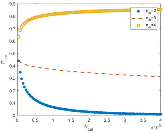
Figure 1. This image shows the probability $P_{sur}$ that cancer does not emerge in an organism as a function of $N_{cell}$ for the different numbers $n_{dr}$ of driver mutations. The probability is computed by relations (53)–(55). The number of cells $N_{cell}$ runs the interval $[1,4M_0]$, where $M_0={10}^9$ (in a typical mouse, the number of cells is $3·M_0$). For each $n_{dr}=2,3,4$, parameter $a_0$ takes values $6.7·{10}^{-4},0.016,0.076$, respectively. The number $T_d$ of cell divisions is $T_d=100$. The parameters are $p_0=0.1a_0$, $\mu =1/3$, and $c_t=1$. We see that the effect dramatically depends on the parameter $n_{dr}$. The mass increase is profitable if $n_{dr}$ is not too small.

The dependence of the survival probability $P_{sur}$ on the stress parameter $\eta$ is complex. The parameter determines the type of stress (such as cooling or heat shock, exposure to toxins, radiation, etc.) and the stress level (for example, concentrations of toxins). The probability of survival depends on $\eta$ through the parameters $a_0,p_0$ (see relation (55)). It is difficult to determine this dependence within the framework of the simple model considered in this section. In the calculations, the parameters were chosen so that the survival probability $P_{sur}$ took on more or less realistic values between 0 and 1. To investigate the dependence $P_{sur}\left(\eta \right)$, we need more advanced spatially extended models, taking into account immune reactions and other phenomena.

10. Concluding Remarks

The three interconnected biological problems are considered: the origins of multicellular organisms, the Peto paradox on cancer and lifespan, and why complex multicellular organisms use a relatively small number of coding genes. The model, proposed in the paper, describes the response of a complex biochemical system to stress and can be viewed as a generalization of the Valiant model of the ideal answer [20]. The Valiant model considers organisms as circuits generating responses to environmental challenges. In the suggested model, some contemporary ideas on cell differentiation, stress response, and morphogenesis are applied, taking into account, to some extent, the real structures of multicellular organisms: biochemical kinetics, decomposition into compartments (tissues), stem cell activity, and gene regulation. It is found that the number of Boolean genes needed to encode an organism does not correlate with the organism’s size. The most intriguing results are obtained in Section 2.5 and Section 2.6. They show that evolutionary success in adaptation does not require fine-tuning genetic networks in differentiated cells of multicellular organisms. To create an effective response to stress, it is enough to correctly encode the interactions between cells. Evolution does not need to have too many genes for this coding. An analysis of the stress response mechanism leads to the conclusion that species with larger organism masses have larger viability: when the mass increases as a linear function, the viability grows as an exponential function. It is important to note that within the same species, we have an inverse dependence: small dogs live longer than large dogs, an effect that is not yet explained.

Complex traits can evolve adaptively or non-adaptively; the discussion regarding the nature of evolution has been ongoing for many years, starting with Kimura’s seminal work [61]; see ([1], 2011) for an overview. Large multicellular organisms form populations of relatively small effective sizes. This suggests that genetic drift in such populations is stronger than in populations formed by prokaryotes. This fact supports the idea that the evolution of these organisms might have been non-adaptive (constructive neutral evolution). The estimates from this paper do not allow us to draw a definite conclusion about the nature of evolution; however, they show that the emergence of multicellular organisms was not completely improbable.

In fact, they show that even a slight increase in network size can exponentially enhance the probability of maintaining homeostasis, provided the initial GRN was sufficiently large. The likelihood of a series of mutations leading to a more efficient network is small, but it is not exponentially small. Even if almost all mutations were non-adaptive, the process of successive replications leading to an organism with complex genetic regulation is possible.

In conclusion, I would like to express my gratitude to the referees for their useful comments and remarks.

Appendix A.1. Estimates for Approximations by RBF

Let us review some results for approximations by radial basis function networks (RBFNs) [33]. Let us introduce a useful notation.

Let ${\mathbb{B}}^d$ be a unit ball in ${\mathbb{R}}^d$ centered at 0, and let $\left|x\right|$ denote the Euclidean norm of the vector $x\in {\mathbb{R}}^d$. Let $p\in (1,+\infty ]$. Let us denote by ${\mathbb{L}}_p\left(D\right)$ the Banach space of all measurable functions on the compact domain $D\subset {\mathbb{R}}^d$ with the norm

$$\left|\right|f\left|\right|={\left({\int }_{D}f{\left(x\right)}^{p}dx\right)}^{1/p}.$$

For $p=+\infty$, we use the supremum norm. The Sobolev class $W_p^r\left(D\right)$ is defined by

$$W_p^r\left(D\right)=\{f:\underset{\mathbf{k},0\le \left|\mathbf{k}\right|\le r}{max}\left|\right|{\mathbf{D}}^{\mathbf{k}}{f\left|\right|}_p<\infty \}$$

where $\mathbf{k}=(k_1,k_2,\dots ,k_d)$ is a multi-index with non-negative integer components, $k_i$, $\left|\mathbf{k}\right|={\sum }_{j=1}^d{k}_j$ and

$${\mathbf{D}}^{\mathbf{k}}f\left(x\right)=\frac{{\partial }^{\left|\mathbf{k}\right|}}{{\partial }^{k_1}{x}_1\dots {\partial }^{k_d}{x}_d}.$$

We denote by $C^r\left(D\right)$ the class of Hölder functions with exponent $r\ge 1$. For two function classes, U and W, the distance between those classes is defined by

$$dist{(U,W)}_p=\underset{f\in U}{sup}\underset{g\in W}{inf}\left|\right|f-{g\left|\right|}_p.$$

The RBFN class ${\mathsf{\Phi }}_{N,\sigma }$ consists of functions of the form

$$F_{net}\left(x\right)=\sum _{j=1}^N{c}_j\sigma (w_j|x-{\overline{x}}_j\left|\right),$$

(A1)

where $c_j,w_j\in \mathbb{R}$ are coefficients, ${\overline{x}}_j$ are localization centers for radial basis function $\sigma \left(z\right)$, which is a well-localized smooth function (for example, a Gaussian peak), and N is the network size.

Appendix A.2. Estimates for RBFN

The following estimate can be obtained (see, for example, [33]):

$$dist(W_p^r\left({\mathbb{B}}^d\right),{\mathsf{\Phi }}_{N,\sigma })<C_{rbf}{N}^{-r/d},$$

(A2)

where a positive constant $C_{rbf}$ depends on p and d only.

Appendix A.3. Encoding GRN

Consider RBF networks $F_{net}$ (see (A1)). We are going to encode the parameters ${\theta }_j,c_i,w_j$ of this network by a binary string s. According to ([13]), for smooth $\sigma$, this binary coding problem can be resolved as follows. Each $c_l$ we approximate by M bits within a precision ${\epsilon }_b<<{ϵ}_k$:

$$|c_l-c_l^b|<{\epsilon }_b,$$

where

$$c_l^b=(1/2-{\overline{s}}_j)\sum _{l=-M_1}^{M_2}{s}_{j,l}{2}^{-l},{\overline{s}}_j,s_{j,l}\in \{0,1\}.$$

Similarly, we proceed for $w_j$ and ${\theta }_j$. We obtain $F_{net,B}$, where all parameters $c_j,w_j,{\theta }_j$ are replaced by their binary approximations. Therefore,

$$\underset{v\in D}{sup}|F_{net}\left(v\right)-F_{net,B}\left(v\right)|<C_1{\epsilon }_b$$

for bounded inputs v and some constants.

Remark. According to [13], for a network $F_{net}$ with size N, we should use $N_g=O\left(N\right){log}_2{\epsilon }_b$ binary genes to construct the network $F_{net,B}$.

Appendix A.4. Estimate of Ventsel–Freidlin Distance

In this subsection, we derive the estimate (46) from the proof of Theorem 1

$${\kappa }^{2}log{P}_{out,\kappa ,N,T}<-C\left(f\right){\delta }^2{\left|\right|g\left|\right|}^{-2}.$$

(A3)

This estimate can be obtained in different ways, and really, it is almost obvious. In fact, if we remove the terms $h_i$ in (23), this equation becomes a linear stochastic equation, which defines a vector-valued Ornstein–Uhlenbeck process. This process is Gaussian with zero mean; hence, it is fully characterized by its covariance matrix. This matrix can be derived in a standard manner, linked to a fundamental physical principle, the fluctuation–dissipation theorem (see, for example, [62]). The second variant involves investigating the Fokker–Planck equation corresponding to (23). For small $\kappa >0$, we can obtain an asymptotic expansion of the solutions of that Fokker–Planck equation at equilibrium. This solution characterizes a probability density function, resembling a slightly perturbed multivariate Gaussian distribution, predominantly localized at the equilibrium.

We use the theory of small random perturbations of dynamical systems developed in ([24], 1984). Let us define the matrix $\mathbf{D}$ with entries $D_{ij}$ by

$$D_{ij}=\sum _{l=1}^p{g}_{il}{g}_{jl}.$$

This matrix is symmetric and positively definite, and ${\mathbf{D}}^{-1}$ exists. We note that

$$({\mathbf{D}}^{-1}w,w)\ge {\left|\right|g\left|\right|}^{-2}{\left|\right|w\left|\right|}^2,$$

(A4)

where w is a vector and $(,),\left|\right|·\left|\right|$ denotes the standard scalar product and the norm in Euclidean space ${\mathbb{R}}^n$. Indeed, let $\tilde{w}={\mathbf{D}}^{-1/2}w$. Then

$$({\mathbf{D}}^{-1}w,w)=({\mathbf{D}}^{-1/2}w,D^{-1/2}w)=\left|\right|\tilde{w}{\left|\right|}^2.$$

By this notation, (A4) can be rewritten as

$$\left|\right|\tilde{w}{\left|\right|}^2\ge {\left|\right|g\left|\right|}^{-2}{\left|\right|w\left|\right|}^2.$$

(A5)

We note that

$${\left|\right|w\left|\right|}^2=\left|\right|{\mathbf{D}}^{1/2}\tilde{w}{\left|\right|}^2=(\mathbf{D}\tilde{w},\tilde{w})={(g,\tilde{w})}^2.$$

(A6)

By the Cauchy–Schwartz inequality,

$${\left|\right|w\left|\right|}^2\le {\left|\right|g\left|\right|}^2\left|\right|\tilde{w}{\left|\right|}^2$$

which is equivalent to (A5).

Let us introduce the Ventsel–Freidlin distance $I(w,v)$ between two points, w and v, by

$$2I(w,v)=\underset{\varphi (·)}{inf}{\int }_0^T\left({\mathbf{D}}^{-1}\left(\mathbf{A}\left(\overline{v}\right)\varphi \left(t\right)+h\left(\varphi \right)+\frac{d\varphi }{dt}\right),\mathbf{A}\left(\overline{v}\right)\varphi \left(t\right)+h\left(\varphi \right)+\frac{d\varphi }{dt}\right)dt,$$

(A7)

where the infimum is taken over all differentiable trajectories $\varphi \left(t\right)$, which connect $\overline{v}$ and v:

$$\varphi \left(0\right)=w,\varphi \left(T\right)=v.$$

According to classical results ([24], 1984), this distance allows one to find an asymptotic estimate of large deviations from the equilibrium for the system (23). We set $w=0$ and let $v\notin W_{\delta }$. Then

$${\kappa }^{2}log{P}_{out}\ge -I(0,v)\kappa \to 0.$$

(A8)

To estimate $I(0,v)$, we define a trajectory $\psi$ defined by

$$\varphi \left(t\right)=exp(-\mathbf{A}t)\psi \left(t\right).$$

Estimate (A4) gives

$$I(0,v)\ge {\left|\right|g\left|\right|}^{-2}\underset{\varphi (·)}{inf}{\int }_0^T\left|\right|\mathbf{A}\left(\overline{v}\right)\varphi \left(t\right)+h\left(\varphi \left(t\right)\right)+\frac{d\varphi }{dt}{\left|\right|}^{2}dt,$$

(A9)

which is equal to

$$I(0,v)\ge {\left|\right|g\left|\right|}^{-2}R,R=\underset{\psi (·)}{inf}{\int }_0^T\left|\right|exp(-\mathbf{A}t)\frac{d\psi }{dt}+h\left(\varphi \left(t\right)\right){\left|\right|}^{2}dt.$$

Using (20) and taking into account $\left|\right|\varphi \left(t\right)\left|\right|\le \delta$ for all $t\in [0,T]$, one has

$$\left|\right|h\left(\varphi \left(t\right)\right)\left|\right|\le {c\left|\right|\varphi \left(t\right)\left|\right|}^2\le c\delta \left|\right|\varphi \left(t\right)\left|\right|$$

which gives

$$I(0,v)\ge R=R_1-R_2,$$

(A10)

where

$$R_1=\underset{\psi (·)}{inf}{\int }_0^T\left|\right|exp(-\mathbf{A}t)\frac{d\psi }{dt}{\left|\right|}^{2}dt$$

and

$$R_2={\delta }^2{\left|\right|exp(-\mathbf{A}t)\psi \left(t\right)\left|\right|}^{2}dt.$$

The relation for $R_1$ can be transformed into

$$R_1=\underset{\psi (·)}{inf}{\int }_0^T(exp(-\mathbf{A}t)\frac{d\psi }{dt},exp(-{\mathbf{A}}^{*}t)\frac{d\psi }{dt})dt,$$

where ${\mathbf{A}}^{*}$ is an operator conjugate to $\mathbf{A}$. One has

$$R=\underset{\psi (·)}{inf}{\int }_0^T\left(exp(-(\mathbf{A}+{\mathbf{A}}^{*})t)\frac{d\psi }{dt},\frac{d\psi }{dt}\right)dt.$$

The operator $\mathbf{L}=\frac{\mathbf{A}+{\mathbf{A}}^{*}}{2}$ is self-adjoint and has negative real-valued eigenvalues; thus, we can use the spectral decomposition. Let ${\mathsf{\Psi }}_n$ be orthogonal eigenfunctions of $\mathbf{L}$, and let ${\lambda }_n\in {\mathbb{R}}_{,{\delta }_{*}}$ be the corresponding eigenvalues. Let us denote the Fourier coefficients by $a_k\left(t\right)=(\psi ,{\mathsf{\Psi }}_k)$. Then

$$R_1\left(a\right)=\sum _{k=1}^n{\int }_0^{T}exp(-2{\lambda }_{k}t){\left(\frac{d{a}_k}{dt}\right)}^{2}dt.$$

(A11)

Similarly,

$$R_2\left(a\right)=\sum _{k=1}^n{\int }_0^{T}exp(-2{\lambda }_{k}t)a_k{\left(t\right)}^{2}dt,$$

(A12)

where $a={(a_1,a_2,\dots ,a_n)}^{\top }$.

We are going to find the minimum of $R\left(a(·)\right)=R_1-R_2$ under the condition $\left|\right|v\left(T\right)\left|\right|\ge \delta$. This condition can be rewritten as

$$\sum _{k=1}^n{a}_k{\left(T\right)}^{2}exp(-2a_{k}T)\ge {\delta }^2.$$

(A13)

This minimization problem can be resolved. The Euler–Lagrange equations have the following form:

$$\frac{d^2{a}_k}{d{t}^2}-2{\lambda }_k\frac{d{a}_k}{dt}-{\delta }^2{a}_k=0.$$

(A14)

They are independent for each k. Solutions of these equations have the following form:

$$a_k\left(t\right)=b_k\left(exp\left({\gamma }_{k}t\right)-exp\left({\tilde{\gamma }}_{k}t\right)\right),$$

where $b_k$ are unknown real numbers and

$${\gamma }_k=2{\lambda }_k+\frac{{\delta }^2}{{\lambda }_k}+O\left({\delta }^4\right),$$

$${\tilde{\gamma }}_k=-\frac{{\delta }^2}{{\lambda }_k}+O\left({\delta }^4\right)$$

for small $\delta >0$. We substitute these relations into (A13) and $R\left(a\right(·\left)\right)$. As a result, we obtain the following minimization problem with respect to unknown coefficients, $b_k$, to find the minimum of

$$R\left(b\right)=\sum _k{b}_k^2{\int }_0^{T}exp(-2{\lambda }_{k}t)\left({\left({\gamma }_{k}exp\left({\gamma }_{k}t\right)-{\tilde{\gamma }}_{k}exp\left({\tilde{\gamma }}_{k}t\right)\right)}^2-{\delta }^2{\left(exp\left({\gamma }_{k}t\right)-exp\left({\tilde{\gamma }}_{k}t\right)\right)}^2\right)dt.$$

under condition

$$\sum _k{b}_k^2{\left(exp\left({\gamma }_{k}T\right)-exp\left({\tilde{\gamma }}_{k}T\right)\right)}^{2}exp(-2{\lambda }_{k}T)\ge {\delta }^2.$$

The minimization problem can be resolved, and we obtain

$$R\ge {\delta }^2{(4min{\lambda }_k)}^{-1}\ge {\delta }^2/4{\delta }_{*}.$$

(A15)

This implies (A3).

References

- Koonin, E.V. The Logic of Chance: The Nature and Origin of Biological Evolution; FT Press: NewYork, NY, USA, 2011. [Google Scholar]
- Iranzo, J.; Lobkovsky, A.E.; Wolf, Y.I.; Koonin, E.V. Virus-host arms race at the joint origin of multicellularity and programmed cell death. Cell Cycle 2014, 13, 3083–3088. [Google Scholar] [CrossRef]
- Koonin, E.V. Viruses and mobile elements as drivers of evolutionary transitions. Phil. Trans. R. Soc. B 2016, 371, 20150442. [Google Scholar] [CrossRef] [PubMed]
- Maynard Smith, J.; Schatzmary, E. The Major Transitions in Evolution; Oxford University Press: Oxford, UK, 1995. [Google Scholar]
- Fisher, R.A. The Genetical Theory of Natural Selection; Clarendon Press: Oxford, UK, 1930. [Google Scholar]
- Orr, H.A. Adaptation and cost of complexity. Evolution 2000, 54, 13–20. [Google Scholar] [CrossRef] [PubMed]
- Orr, H.A. The genetic theory of adaptation: A brief history. Nat. Rev. Genet. 2005, 6, 119–127. [Google Scholar] [CrossRef] [PubMed]
- Peto, R.; Roe, F.J.C.; Lee, P.N.; Levy, L.; Clack, J. Cancer and ageing in mice and men. Br. J. Cancer 1975, 32, 411–426. [Google Scholar] [CrossRef] [PubMed]
- Caulin, A.F.; Maley, C.C. Peto’s Paradox: Evolution’s prescription for cancer prevention. Trends Ecol. Evol. 2011, 26, 175–182. [Google Scholar] [CrossRef]
- Kobayashi, H.; Man, S. cquired multicellular-mediated resistance to alkylating agents in cancer. Proc. Natl. Acad. Sci. USA 1993, 90, 3294–3298. [Google Scholar] [CrossRef]
- Domazet-Loso, T.; Tautz, D. Phylostratigraphic tracking of cancer genes suggests a link to the emergence of multicellularity in metazoa. BMC Biol. 2010, 8, 66. [Google Scholar] [CrossRef]
- Dang, C. Links between metabolism and cancer. Genes Dev. 2012, 26, 877–890. [Google Scholar] [CrossRef]
- Vakulenko, S.; Grigoriev, D. Deep gene networks and response to stress. Mathematics 2021, 9, 3028. [Google Scholar] [CrossRef]
- Hansberg, W.; Aguirre, J.; Rís-Momberg, M.; Rangel, P.; Peraza, L.; Montes de Oca, Y.; Cano-Domínguez, N. Cell differentiation as a response to oxidative stress. Br. Mycol. Soc. Symp. Ser. 2008, 27, 235–257. [Google Scholar]
- Tower, J. Stress and stem cells. Wiley Interdiscip. Rev. Dev. Biol. 2012, 1, 789–802. [Google Scholar] [CrossRef] [PubMed]
- Bornstein, S.; Steenblock, C.; Chrousos, G.P.; Schally, A.V.; Beuschlein, F.; Kline, G.; Krone, N.P.; Licinio, J.; Wong, M.L.; Ullmann, E.; et al. Stress-inducible-stem cells: A new view on endocrine, metabolic and mental disease? Mol. Psychiatry 2019, 24, 2–9. [Google Scholar] [CrossRef] [PubMed]
- Greaves, R.B.; Dietmann, S.; Smith, A.; Stepney, S.; Halley, J.D. A conceptual and computational framework for modelling and understanding the non-equilibrium gene regulatory networks of mouse embryonic stem cells. PLoS Comput. Biol. 2017, 13, e1005713. [Google Scholar] [CrossRef]
- Jiang, P.; Ludwig, M.L.; Kreitman, M.; Reinitz, J. Natural variation of the expression pattern of the segmentation gene even-skipped in Drosophila melanogaster. Dev. Biol. 2015, 405, 173–181. [Google Scholar] [CrossRef]
- Mjolsness, E.; Sharp, D.H.; Reinitz, J. A connectionist model of development. J. Theor. Biol. 1991, 152, 429–453. [Google Scholar] [CrossRef]
- Valiant, L.G. Evolvability. J. ACM 2006, 120, 1–19. [Google Scholar]
- Vakulenko, S.; Grigoriev, D. Instability, complexity, and evolutionz. Zap. Nauchn. Sem. POMI 2008, 360, 31–69. [Google Scholar]
- Gromov, M.; Carbone, A. Mathematical slices of molecular biology. Gaz. MathéMaticiens 2001, 88A. [Google Scholar]
- Vakulenko, S. Complexity and Evolution of Dissipative Systems; de Gruyter: Berlin, Germany, 2014. [Google Scholar]
- Ventsel, D.A.; Freidlin, M.I. Random Perturbations of Dynamic Systems; Springer: New York, NY, USA, 1984. [Google Scholar]
- Reinitz, J.; Sharp, D.H. Mechanism of formation of eve stripes. Mech. Dev. 1995, 49, 133–158. [Google Scholar] [CrossRef]
- Valiant, L.G. Evolvability. J. ACM 2009, 56, 1–21. [Google Scholar] [CrossRef]
- Horsthemke, W.; Lefever, R. Noise-induced Transitions; Springer: Berlin/Heidelberg, Germany, 1984. [Google Scholar]
- Chen, B.; Abuassba, A.O. Compartmental Models with Application to Pharmacokinetics. Procedia Comput. Sci. 2021, 187, 60–70. [Google Scholar] [CrossRef]
- Gillespie, D.T. Exact Stochastic Simulation of Coupled Chemical Reactions. J. Phys. Chem. 1977, 81, 2340–2361. [Google Scholar] [CrossRef]
- Henry, D. Geometric Theory of Semilinear Parabolic Equations; Springer: Berlin/Heidelberg, Germany, 1981. [Google Scholar]
- Szendro, I.G.; Schenk, M.F.; Franke, J.; Krug, J.; de Visser, J.A.G. Quantitative analyses of empirical fitness landscapes. J. Stat. Mech. Theory Exp. 2013, 2013, P01005. [Google Scholar] [CrossRef]
- Jiang, P.; Reinitz, J.; Kreitman, M. The effect of mutational robustness on the evolvability of multicellular organisms and eukaryotic cells. J. Evol. Biol. 2023, 36, 906–924. [Google Scholar] [CrossRef] [PubMed]
- Lin, S.; Liu, X.; Rong, Y.; Xu, Z. Almost optimal estimates for approximation and learning by radial basis function networks. Mach. Learn. 2014, 95, 147–164. [Google Scholar] [CrossRef]
- Turing, A. The chemical basis of morphogenesis. Phil. Trans. Roy. Soc. B 1952, 237, 37–72. [Google Scholar]
- Cooke, J.; Zeeman, E. A Clock and Wavefront model for control of the number of repeated structures during animal morphogenesis. J. Theor. Biol. 1976, 58, 455–476. [Google Scholar] [CrossRef]
- Meinhardt, H. Models of Biological Pattern Formation; Academic Press: London, UK, 1982; pp. 1–215. [Google Scholar]
- Baker, R.; Schnell, S.; Maini, P. A clock and wavefront mechanism for somite formation. Dev. Biol. 2006, 293, 116–126. [Google Scholar] [CrossRef]
- Kishan, K.; Rui, L.; Cui, F.; Yu, Q.; Haake, A.R. GNE: A deep learning framework for gene network inference by aggregating biological information. BMC Syst. Biol. 2019, 13, 38. [Google Scholar]
- Shen, Z.; Yang, H.; Zhang, S. Nonlinear Approximation via Compositions. Neural Netw. 2019, 119, 74–84. [Google Scholar] [CrossRef] [PubMed]
- Surkova, S.; Spirov, A.V.; Gursky, V.V.; Janssens, H.; Kim, A.R.; Radulescu, O.; Vanario-Alonso, C.E.; Sharp, D.H.; Samsonova, M.; Reinitz, J.; et al. Canalization of gene expression in the Drosophila blastoderm by gap gene cross regulation. PLoS Biol. 2009, 7, e1000049. [Google Scholar]
- Murray, J.D. Mathematical Biology, 3rd ed.; Springer: Berlin/Heidelberg, Germany, 2002. [Google Scholar] [CrossRef]
- Crampin, E.J.; Gaffney, E.A.; Maini, P.K. Reaction and diffusion on growing domains: Scenarios for robust pattern formation. Bull. Math. Biol. 1999, 61, 1093–1120. [Google Scholar] [CrossRef] [PubMed]
- Krause, A.L.; Gaffney, E.A.; Maini, P.K.; Kika, V. Modern Perspectives on Near-Equilibrium Analysis of Turing Systems. Philos. Trans. A 2019, 379, 20200268. [Google Scholar] [CrossRef]
- Nicolis, G.; Prigogine, I. Self-Organization in Nonequilibrium Systems: From Dissipative Structures to Order through Fluctuations; Wiley and Sons: New York, NY, USA; London, UK; Sydney, Australia; Toronto, ON, Canada, 1977. [Google Scholar]
- Haken, H. Synergetics: An Introduction: Nonequilibrium Phase Transitions and Self-Organization in Physics, Chemistry, and Biology; Springer: Berlin/Heidelberg, Germany; New York, NY, USA, 1978. [Google Scholar]
- Vakulenko, S.; Volpert, V. Generalized travelling waves for perturbed monotone reaction-diffusion systems. Nonlinear Anal. 2001, 46, 757–776. [Google Scholar] [CrossRef]
- Brenner, S. Life’s code script. Nature 2012, 482, 461. [Google Scholar] [CrossRef]
- Maroto, M.; Bone, R.A.; Dale, J. Somitogenesis. Development 2012, 139, 2453–2456. [Google Scholar] [CrossRef]
- Resende, T.; Ferreira, M.; Teillet, M.A.; Tavares, A.T.; Andrade, R.P.; Palmeirim, I. Sonic hedgehog in temporal control of somite formation. Proc. Natl. Acad. Sci. USA 2010, 107, 12907–12912. [Google Scholar] [CrossRef]
- Pourquié, O. The chick embryo: A leading model for model in somitogenesis studies. Mech. Dev 2004, 121, 1069–1079. [Google Scholar] [CrossRef]
- Heltberg, M.L.; Krishna, S.; Jensen, M. On chaotic dynamics in transcription factors and the associated effects in differential gene regulation. Nat. Commun. 2019, 10, 71. [Google Scholar] [CrossRef]
- Wolpert, L.; Tickle, C.; Jessell, T. Principles of development; Oxford University Press: Cambridge, UK, 2002. [Google Scholar]
- Reinitz, J.; Vakulenko, S.; Sudakow, I.; Grigoriev, D. Robust morphogenesis by chaotic dynamics. Sci. Rep. 2023, 13, 7482. [Google Scholar] [CrossRef] [PubMed]
- Maroudas-Sacks, Y.; Keren, K. Mechanical Patterning in Animal Morphogenesis. Annu. Rev. Cell Dev. Biol. 2021, 37, 469–493. [Google Scholar] [CrossRef] [PubMed]
- Sudakow, I.; Vakulenko, S.; Grigoriev, D. Excitable media store and transfer complicated information via topological defect motion. Commun. Nonlinear Sci. Numer. Simul. 2023, 116, 106844. [Google Scholar] [CrossRef]
- Vakulenko, S.; Grigoriev, D. Complexity of gene circuits, Pfaffian functions and the morphogenesis problem. Compte Rendu Math. 2003, 337, 721–724. [Google Scholar] [CrossRef]
- Vakulenko, S.; Radulescu, O.; Reinitz, J. Size Regulation in the Segmentation of Drosophila: Interacting Interfaces between Localized Domains of Gene Expression Ensure Robust Spatial Patterning. Phys. Rev. Lett. 2009, 103, 168102–168106. [Google Scholar] [CrossRef]
- Iranzo, J.; Martincorena, I.; Koonin, E. Cancer-mutation network and the number and specificity of driver mutations. Proc. Natl. Acad. Sci. USA 2018, 115, E6010–E6019. [Google Scholar] [CrossRef]
- Longa, H.; Miller, S.F.; Strauss, C.; Zhao, C.; Cheng, L.; Ye, Z.; Griffin, K.; Te, R.; Lee, H.; Chen, C.; et al. Antibiotic treatment enhances the genome-wide mutation rate of target cells. Proc. Natl. Acad. Sci. USA 2016, 113. [Google Scholar] [CrossRef]
- Milholland, B.; Dong, X.; Zhang, L.; Hao, X.; Suh, Y.; Vijg, J. Differences between germline and somatic mutation rates in humans and mice. Nat Commun. 2017, 8, 15183. [Google Scholar] [CrossRef]
- Kimura, M. The Neutral Theory of Molecular Evolution; Cambridge University Press: Cambridge, UK, 1983. [Google Scholar]
- Keizer, J. Statistical Thermodynamics of Nonequilibrium Processes; Springer: New York, NY, USA, 1987. [Google Scholar]
Disclaimer/Publisher’s Note: The statements, opinions and data contained in all publications are solely those of the individual author(s) and contributor(s) and not of MDPI and/or the editor(s). MDPI and/or the editor(s) disclaim responsibility for any injury to people or property resulting from any ideas, methods, instructions or products referred to in the content. |
© 2023 by the author. Licensee MDPI, Basel, Switzerland. This article is an open access article distributed under the terms and conditions of the Creative Commons Attribution (CC BY) license (https://creativecommons.org/licenses/by/4.0/).