Global Dynamics in an Alcoholism Epidemic Model with Saturation Incidence Rate and Two Distributed Delays

Abstract

In this study, considering the delays for a susceptible individual becoming an alcoholic and the relapse of a recovered individual back into being an alcoholic, we formulate an epidemic model for alcoholism with distributed delays and relapse. The basic reproduction number $R_0$ is calculated, and the threshold property of $R_0$ is established. By analyzing the characteristic equation, we demonstrate the local asymptotic stability of the different equilibria under various conditions: when $R_0<1$, the alcoholism-free equilibrium is locally asymptotically stable; when $R_0>1$, the alcoholism equilibrium exists and is locally asymptotically stable. Furthermore, we demonstrate the global asymptotic stability at each equilibrium using a suitable Lyapunov function. Specifically, when $R_0<1$, the alcoholism-free equilibrium is globally asymptotically stable; when $R_0>1$, the alcoholism equilibrium is globally asymptotically stable. The sensitivity analysis of $R_0$ shows that reducing exposure is more effective than treatment in controlling alcoholism. Interestingly, we found that extending the latency delay $h_1$ and relapse delay $h_2$ also effectively contribute to the control of the spread of alcoholism. Numerical simulations are also provided to support our theoretical results.

1. Introduction and Model Formulation

Alcoholism, also known as alcohol dependence, is a pervasive social issue. It is characterized by an individual’s uncontrollable desire for alcohol, potential physical dependence on it, and an inability to recognize the negative consequences of excessive drinking [1,2]. According to the World Health Organization (WHO) estimates, globally, the detrimental use of alcohol results in three million deaths annually, accounting for 5.3% of all deaths [3]. The harmful use of alcohol is a causal factor in more than 200 disease and injury conditions [4]. Such problems include health complications, unemployment, and instances of domestic violence, among others [5]. Furthermore, alcohol abuse, which is considered the third-most-significant risk factor for illness and disability worldwide, contributes to 60 separate diseases [6,7,8]. Teenage alcohol abuse is particularly concerning. Surveys in the United States show two significant trends. Over 40% of college students have engaged in binge drinking [9,10]. In addition, approximately 90% have had at least one alcohol-related experience [11]. Moreover, there is a growing concern that a significant proportion of individuals who abuse alcohol are likely to relapse even after undergoing treatment. Presently, the detrimental effects of excessive alcohol consumption extend beyond health issues, severely affecting social security as well. Therefore, developing effective strategies to combat alcoholism has become an urgent issue that demands immediate attention.

The propagation of alcohol-related behaviors exhibits characteristics analogous to the transmission dynamics of infectious diseases. Consequently, the application of mathematical models traditionally used in infectious disease epidemiology has become a notable method in alcoholism research. Numerous models related to alcoholism have been developed and analyzed. For instance, Benedict [12] modeled alcoholism as an infectious disease and proposed an alcoholism model. In this model, the population of drinkers is segmented into three groups: susceptible drinkers, alcoholics, and recovered individuals. Benedict further explored how alcoholic behavior spread among these groups. Mubayi et al. [13] characterized alcohol consumption as a social contagion process. They revealed that the relative duration that moderate drinkers stay in different environments has a significant impact on the proportion of heavy drinkers. In another study [14], a two-stage (four-component) model of youth alcoholism was introduced. This model categorized binge drinking youths into two groups: those who self-admitted to binge drinking and those who denied such behavior. It identified a threshold and conducted an analysis of the stability of the system. Then, Huo et al. [15] incorporated a direct transfer from the susceptible compartment to the admitted alcoholic compartment and established the global dynamical behaviors of the system. Manthey et al. [16] focused on alcohol-related problems on college campuses and developed a campus drinking model. Their findings highlighted the significant role that the ability of alcoholics in recruiting new members plays in such issues. In other works [17,18], the authors took into account the time period required for non-consumers to become alcohol consumers and formulated an epidemic model of alcoholism with time delay. Allsop et al. [19] noted that abstaining from alcohol is often temporary. Despite numerous individuals with alcohol-related problems achieving recovery through treatment, they are susceptible to relapse when exposed to others who consume alcohol excessively. In more recent studies [2,20,21], the authors studied the spread model of alcoholism with relapse, introducing a relapse term into the model and analyzing its dynamics. Djillali et al. [22] considered the varying time needed for those returning to alcohol consumption from a treatment program, proposing an epidemic model of alcoholism with distributed delays, as follows:

$$\left\{\begin{array}{cc}\hfill {\displaystyle \frac{\mathrm{d}S}{\mathrm{d}t}}=& \Lambda -\beta S\left(t\right)H\left(t\right)-\left(\mu +\alpha \right)S\left(t\right),\hfill \\ \hfill {\displaystyle \frac{\mathrm{d}H}{\mathrm{d}t}}=& \beta S\left(t\right)H\left(t\right)+\alpha S\left(t\right)-\left(\mu +\eta +\delta \right)H\left(t\right)+{\int }_0^{\tau }k\left(\sigma \right)e^{-\left(\mu +d\right)\sigma }\delta H\left(t-\sigma \right)d\sigma ,\hfill \\ \hfill {\displaystyle \frac{\mathrm{d}R}{\mathrm{d}t}}=& \delta H\left(t\right)-\left(\mu +d\right)R\left(t\right)-{\int }_0^{\tau }k\left(\sigma \right)e^{-\left(\mu +d\right)\sigma }\delta H\left(t-\sigma \right)d\sigma ,\hfill \end{array}\right.$$

(1)

where $S\left(t\right)$, $H\left(t\right)$, and $R\left(t\right)$ denote the densities of susceptible individuals, alcoholics, and recovered individuals, respectively. $\Lambda >0$ denotes the rate at which individuals enter the susceptible population; $\mu$ represents the natural death rate; $\beta$ signifies the transmission coefficient from the susceptible population to alcoholics; $\delta$ represents the rate at which alcoholics enter into treatment. $\eta$ denotes the death rate due to excessive alcohol consumption; d represents the proportion of individuals who have completely quit drinking after undergoing treatment. Lastly, $\alpha$ represents the rate of individuals becoming addicted due to societal influences. The relapse term is

$${\int }_0^{\tau }k\left(\sigma \right)e^{-\left(\mu +d\right)\sigma }\delta H\left(t-\sigma \right)d\sigma ={\int }_{t-\tau }^{t}k\left(t-\eta \right)e^{-\left(\mu +d\right)\left(t-\eta \right)}\delta H\left(\eta \right)d\eta ,$$

where the kernel $k\left(\sigma \right)$ represents the probability distribution of delay. $\tau$ is the maximum duration spent in the recovered stage before an individual becomes fully recovered, with ${\int }_0^{\tau }k\left(\sigma \right)d\sigma =1$.

Inspired by the aforementioned work, we propose that a susceptible individual, after coming into contact with an alcoholic, will not be immediately influenced, as the habit of alcohol consumption takes time to develop. Similarly, an individual who has received treatment will not instantly relapse; it requires a period of time before potentially relapsing into being an alcoholic. Therefore, we introduced the concept of delay for both susceptible individuals becoming alcoholics and recovered individuals relapsing into alcoholics. In situations of heightened infection levels, the probability of individual contact may decrease due to the self-protective psychological effects or inhibitory behaviors of the susceptible individuals. Therefore, we introduce the saturation incidence rate and, subsequently, formulate the following model:

$$\left\{\begin{array}{cc}\hfill {\displaystyle \frac{\mathrm{d}S}{\mathrm{d}t}}=& \Lambda -\frac{\beta S\left(t\right)H\left(t\right)}{1+\theta H\left(t\right)}-\mu S\left(t\right),\hfill \\ \hfill {\displaystyle \frac{\mathrm{d}E}{\mathrm{d}t}}=& \frac{\beta S\left(t\right)H\left(t\right)}{1+\theta H\left(t\right)}-\beta {\int }_0^{h_1}{f}^{\prime }\left(\sigma \right)\frac{S(t-\sigma )H(t-\sigma )}{1+\theta H(t-\sigma )}{e}^{-\mu \sigma }d\sigma -\mu E\left(t\right),\hfill \\ \hfill {\displaystyle \frac{\mathrm{d}H}{\mathrm{d}t}}=& \beta {\int }_0^{h_1}{f}^{\prime }\left(\sigma \right)\frac{S(t-\sigma )H(t-\sigma )}{1+\theta H(t-\sigma )}{e}^{-\mu \sigma }d\sigma +\delta {\int }_0^{h_2}{g}^{\prime }\left(\sigma \right)H(t-\sigma )e^{-(\mu +d)\sigma }d\sigma \hfill \\ \hfill & -\mu H\left(t\right)-\delta H\left(t\right)-\eta H\left(t\right),\hfill \\ \hfill {\displaystyle \frac{\mathrm{d}R}{\mathrm{d}t}}=& \delta H\left(t\right)-\delta {\int }_0^{h_2}{g}^{\prime }\left(\sigma \right)H(t-\sigma )e^{-(\mu +d)\sigma }d\sigma -\mu R\left(t\right)-dR\left(t\right).\hfill \end{array}\right.$$

(2)

In the model, $E\left(t\right)$ represents the individuals who have been exposed to, but have not yet developed a habit of alcoholism. $\theta$ is referred to as the psychological factor, which can reflect the behavior changes caused by the psychological effects on individuals. The term $h_1$ denotes the maximum duration of the latent period delay, while $h_2$ signifies the maximum duration of the relapse delay.

The function $f^{\prime }\left(\sigma \right)$ represents the distribution of an alcoholic’s infectivity among susceptible individuals, where the duration required for an individual to become an alcoholic is $\sigma$. This function is continuous, non-negative, and satisfies ${\int }_0^{h_1}{f}^{\prime }\left(\sigma \right)d\sigma =1$. The function $g^{\prime }\left(\sigma \right)$ signifies the distribution of relapse among those in treatment, where the duration required for an individual to relapse into an alcoholic from treatment is $\sigma$. This function is continuous, non-negative, and satisfies ${\int }_0^{h_2}{g}^{\prime }\left(\sigma \right)d\sigma =1$. The term $e^{-\mu \sigma }$ represents the survival probability of an alcoholic who originated from the susceptible population; $e^{-(\mu +d)\sigma }$ signifies the survival probability of an alcoholic during his/her relapse from treatment.

Let us set ${\omega }_1=t-\sigma$. Following from this, we have

$$\beta {\int }_0^{h_1}{f}^{\prime }\left(\sigma \right)\frac{S(t-\sigma )H(t-\sigma )}{1+\theta H(t-\sigma )}{e}^{-\mu \sigma }d\sigma =\beta {\int }_{t-h_1}^t{f}^{\prime }(t-{\omega }_1)\frac{S\left({\omega }_1\right)H\left({\omega }_1\right)}{1+\theta H\left({\omega }_1\right)}{e}^{-\mu (t-{\omega }_1)}d{\omega }_1.$$

This term denotes the susceptible who became infected at ${\omega }_1({\omega }_1\in [t-h_1,t])$ and became alcoholic at time t. Furthermore, we set ${\omega }_2=t-\sigma ({\omega }_2\in [t-h_2,t])$:

$$\delta {\int }_0^{h_2}{g}^{\prime }\left(\sigma \right)H(t-\sigma )e^{-(\mu +d)\sigma }d\sigma =\delta {\int }_{t-h_2}^t{g}^{\prime }(t-{\omega }_2)H\left({\omega }_2\right)e^{-(\mu +d)(t-{\omega }_2)}d{\omega }_2.$$

This term represents the relapse term.

The initial conditions for the model are as follows:

$$S\left(\alpha \right)={\phi }_1\left(\alpha \right),E\left(\alpha \right)={\phi }_2\left(\alpha \right),H\left(\alpha \right)={\phi }_3\left(\alpha \right),R\left(\alpha \right)={\phi }_4\left(\alpha \right),$$

(3)

where ${\phi }_i\left(\alpha \right)\ge 0,\alpha \in [-h,0]$, ${\phi }_i\left(0\right)>0(i=1,2,3,4)$. Here $h=max\{h_1,h_2\}$, $({\phi }_1\left(\alpha \right),{\phi }_2\left(\alpha \right),$${\phi }_3\left(\alpha \right),{\phi }_4\left(\alpha \right))\in C([-h,0],{\mathbb{R}}_{+}^4)$.

For the convenience of the following proof, we let $f\left(\sigma \right)=f^{\prime }\left(\sigma \right)e^{-\mu \sigma }$, $g\left(\sigma \right)=g^{\prime }\left(\sigma \right)e^{-(\mu +d)\sigma }$.

2. Preliminary Analysis of the Model

2.1. Positivity of Solutions and Invariant Region

In this section, we aim to demonstrate that the alcoholism epidemic model is epidemiologically meaningful. We will do this by introducing the non-negativity and boundedness of the solution of the system.

Lemma 1.

Assume that $S\left(t\right)$, $E\left(t\right)$, $H\left(t\right)$, and $R\left(t\right)$ are solutions of the system $\left(2\right)$, given certain initial conditions $\left(3\right)$. Then, $S\left(t\right)\ge 0$, $E\left(t\right)\ge 0$, $H\left(t\right)\ge 0$, and $R\left(t\right)\ge 0$ for all $t\ge 0$.

Proof. 

First, we prove that $S\left(t\right)\ge 0$ for all t. Assume the contrary, that there exists $t_1$ such that $S\left(t_1\right)<0$. We set $t_2=inf\{0<t<t_1:S\left(t\right)<0\}$. Then, we have $S\left(t_2\right)=0$. From the first equation of the system $\left(2\right)$, we conclude that ${\left.{\displaystyle \frac{dS}{dt}}\right|}_{t=t_2}>0$. Hence, we find $S\left(t\right)<0$ for $t\in \left(t_2-\epsilon ,t_2\right)$, where $\epsilon$ is a positive, sufficiently small number. This contradicts our earlier finding that $S\left(t\right)\ge 0$ for $t\in \left(0,t_2\right]$. Therefore, we must have $S\left(t\right)\ge 0$ for all t.

Next, to prove that $H\left(t\right)\ge 0$, in fact, we assume the contrary, and let $t_3>0$, such that $H\left(t_3\right)<0$, and set $t_4=inf\{0<t<t_3:H\left(t\right)<0\}$. Then, we have $H\left(t_4\right)=0$.

Let

$$\begin{array}{c}\hfill a\left(t\right)=\beta {\int }_0^{h_1}f\left(\sigma \right)\frac{S(t-\sigma )H(t-\sigma )}{1+\theta H(t-\sigma )}d\sigma +\delta {\int }_0^{h_2}g\left(\sigma \right)H(t-\sigma )d\sigma .\end{array}$$

Considering that $S\left(t\right)\ge 0$ and $H\left(t\right)\ge 0$ for $t\in (-h,t_4)$, where $h=max(h_1,h_2)$, consequently, it follows that $a\left(t\right)\ge 0$ for $t\in (-h,t_4)$. Using an integrating factor for the third equation of the system $\left(2\right)$ gives

$$\begin{array}{c}\hfill H\left(t\right)=\left[H\left(0\right)+{\int }_0^{t}a\left(\xi \right)e^{\left(\mu +\delta +\eta \right)\xi }d\xi \right]e^{-\left(\mu +\delta +\eta \right)t};\end{array}$$

combining $H\left(0\right)={\phi }_2\left(0\right)>0$, we can derive that

$$\begin{array}{c}\hfill H\left(t_4\right)=\left[H\left(0\right)+{\int }_0^{t_4}a\left(\xi \right)e^{(\mu +\delta +\eta )\xi }d\xi \right]e^{-(\mu +\delta +\eta )t_4}>0.\end{array}$$

This contradicts $H\left(t_4\right)=0$; therefore, $H\left(t\right)\ge 0$ for all $t\ge 0$. Similarly, we can obtain $E\left(t\right)\ge 0$, $R\left(t\right)\ge 0$ for all $t\ge 0$. □

Define

$$\begin{array}{c}\hfill D=\left\{\left(S\left(t\right),E\left(t\right),H\left(t\right),R\left(t\right)\right):S\left(t\right)\ge 0,E\left(t\right)\ge 0,H\left(t\right)\ge 0,R\left(t\right)\ge 0,S\left(t\right)+E\left(t\right)+H\left(t\right)+R\left(t\right)\le {\displaystyle \frac{\Lambda }{\mu }}\right\}.\end{array}$$

Lemma 2.

Let $\left(S\right(t),E(t),H(t),R(t\left)\right)$ be the solution of the system $\left(2\right)$, with an initial condition $\left(3\right)$ in D. Then, the solution remains in D.

Proof. 

The non-negativity of $\left(S\right(t),E(t),H(t),R(t\left)\right)$ follows from Lemma 1.

Next, by adding all the equations in the system $\left(2\right)$, we obtain ${(S\left(t\right)+E\left(t\right)+H\left(t\right)+R\left(t\right))}^{\prime }\le \Lambda -\mu (S\left(t\right)+E\left(t\right)+H\left(t\right)+R\left(t\right))$. Thus, $\underset{t\to \infty }{lim}sup\left(S\left(t\right)+E\left(t\right)+H\left(t\right)+R\left(t\right)\right)\le {\displaystyle \frac{\Lambda }{\mu }}$.

It follows that the solutions are bounded and remain in D. □

2.2. Equilibrium and Basic Reproduction Number

Since E and R are completely determined by S and H, we only need to study the dynamics of the following system:

$$\left\{\begin{array}{cc}\hfill {\displaystyle \frac{\mathrm{d}S}{\mathrm{d}t}}=& \Lambda -\frac{\beta S\left(t\right)H\left(t\right)}{1+\theta H\left(t\right)}-\mu S\left(t\right),\hfill \\ \hfill {\displaystyle \frac{\mathrm{d}H}{\mathrm{d}t}}=& \beta {\int }_0^{h_1}f\left(\sigma \right)\frac{S(t-\sigma )H(t-\sigma )}{1+\theta H(t-\sigma )}d\sigma +\delta {\int }_0^{h_2}g\left(\sigma \right)H(t-\sigma )d\sigma \hfill \\ \hfill & -\mu H\left(t\right)-\delta H\left(t\right)-\eta H\left(t\right).\hfill \end{array}\right.$$

(4)

Next, we calculate the basic reproduction number $R_0$ for the spread of alcoholism. Here, the basic reproduction number refers to the expected number of second-generation alcoholics produced by a single alcoholic individual during their influential period in a completely susceptible population. It is used to measure the transmissibility of alcoholism and provides an important basis for determining the prevalence and extinction of the issue of alcoholism within a population. Following the method of the next-generation approach developed by van den Driessche and Watmough [23], we can obtain

$$\begin{array}{c}\hfill \begin{array}{c}\mathcal{F}=\left[\begin{array}{c}{\mathcal{F}}_1\\ {\mathcal{F}}_2\end{array}\right]=\left[\begin{array}{c}\beta {\int }_0^{h_1}f\left(\sigma \right){\displaystyle \frac{S(t-\sigma )H(t-\sigma )}{1+\theta H(t-\sigma )}}d\sigma \\ 0\end{array}\right],\hfill \\ \mathcal{V}=\left[\begin{array}{c}{\mathcal{V}}_1\\ {\mathcal{V}}_2\end{array}\right]=\left[\begin{array}{c}-\delta {\int }_0^{h_2}g\left(\sigma \right)H(t-\sigma )d\sigma +\mu H\left(t\right)+\delta H\left(t\right)+\eta H\left(t\right)\\ -\Lambda +{\displaystyle \frac{\beta S\left(t\right)H\left(t\right)}{1+\theta H\left(t\right)}}+\mu S\left(t\right)\end{array}\right],\hfill \end{array}\end{array}$$

(5)

where ${\mathcal{F}}_i$ is the rate of appearance of new infections in a compartment and ${\mathcal{V}}_i$ represents the rate of individual input and output through other means in a compartment $i=1,2$, then

$$\begin{array}{cc}\hfill F=& \frac{\partial {\mathcal{F}}_1}{\partial H}\left(P_0\right)=\beta \frac{\Lambda }{\mu }{\int }_0^{h_1}f\left(\sigma \right)d\sigma ,\hfill \\ \hfill V=& \frac{\partial {\mathcal{V}}_1}{\partial H}\left(P_0\right)=\mu +\delta +\eta -\delta {\int }_0^{h_2}g\left(\sigma \right)d\sigma ;\hfill \end{array}$$

(6)

therefore, we obtain

$$\begin{array}{c}\hfill R_0={\displaystyle \frac{\beta \Lambda {\int }_0^{h_1}f\left(\sigma \right)d\sigma }{\mu \left(\delta +\mu +\eta -\delta {\int }_0^{h_2}g\left(\sigma \right)d\sigma \right)}}.\end{array}$$

(7)

To study the dynamical behaviors of the system $\left(4\right)$, it is necessary to find both the alcoholism-free equilibrium and the alcoholism equilibrium. By setting ${\displaystyle \frac{\mathrm{d}S}{\mathrm{d}t}}=0$ and ${\displaystyle \frac{\mathrm{d}H}{\mathrm{d}t}}=0$, we can obtain the alcoholism-free equilibrium $P_0=(S^0,H^0)=\left({\displaystyle \frac{\Lambda }{\mu }},0\right)$ and the alcoholism equilibrium $P_{*}=(S^{*},H^{*})$, where

$$\left\{\begin{array}{cc}\hfill S^{*}=& {\displaystyle \frac{\delta +\mu +\eta -\delta {\int }_0^{h_2}g\left(\sigma \right)d\sigma +\theta \Lambda {\int }_0^{h_1}f\left(\sigma \right)d\sigma }{\left(\beta +\mu \theta \right){\int }_0^{h_1}f\left(\sigma \right)d\sigma }},\hfill \\ \hfill H^{*}=& {\displaystyle \frac{\beta \Lambda {\int }_0^{h_1}f\left(\sigma \right)d\sigma -\mu \left(\delta +\mu +\eta -\delta {\int }_0^{h_2}g\left(\sigma \right)d\sigma \right)}{\left(\beta +\mu \theta \right)\left(\delta +\mu +\eta -\delta {\int }_0^{h_2}g\left(\sigma \right)d\sigma \right)}}.\hfill \end{array}\right.$$

(8)

Further simplifying, we obtain $S^{*}=\left(\theta +{\displaystyle \frac{\beta }{\mu R_0}}\right){\displaystyle \frac{\Lambda }{\beta +\mu \theta }}$, $H^{*}=\mu (R_0-1){\displaystyle \frac{1}{\beta +\mu \theta }}$, where $R_0={\displaystyle \frac{\beta \Lambda {\int }_0^{h_1}f\left(\sigma \right)d\sigma }{\mu \left(\delta +\mu +\eta -\delta {\int }_0^{h_2}g\left(\sigma \right)d\sigma \right)}}={\displaystyle \frac{\beta S^0{\int }_0^{h_1}f\left(\sigma \right)d\sigma }{\delta +\mu +\eta -\delta {\int }_0^{h_2}g\left(\sigma \right)d\sigma }}$.

3. Locally Asymptotic Stability of Equilibrium

3.1. Locally Asymptotic Stability of the Alcoholism-Free Equilibrium

Theorem 1.

The alcoholism-free equilibrium $P_0=(S^0,H^0)$ of the system $\left(4\right)$ is locally asymptotically stable if $R_0<1$ and unstable if $R_0>1$.

Proof. 

The linear dynamics system of $\left(4\right)$ at $P_0$ can be written as

$$\left\{\begin{array}{cc}\hfill {\displaystyle \frac{\mathrm{d}S}{\mathrm{d}t}}=& -\beta S^{0}H\left(t\right)-\mu S\left(t\right),\hfill \\ \hfill {\displaystyle \frac{\mathrm{d}H}{\mathrm{d}t}}=& \beta S^0{\int }_0^{h_1}f\left(\sigma \right)H(t-\sigma )d\sigma +\delta {\int }_0^{h_2}g\left(\sigma \right)H(t-\sigma )d\sigma \hfill \\ \hfill & -\delta H\left(t\right)-\mu H\left(t\right)-\eta H\left(t\right).\hfill \end{array}\right.$$

(9)

The characteristic equation of the system $\left(9\right)$ can be derived by seeking for exponential solutions. Let $S\left(t\right)=\overline{X}{e}^{\lambda t}$, $H\left(t\right)=\overline{Y}{e}^{\lambda t}$, where $\overline{X}$ and $\overline{Y}$ are the undetermined coefficients, then substituting these expressions into the linearized system $\left(9\right)$, we can obtain

$$\left\{\begin{array}{cc}\hfill & (\lambda +\mu )\overline{X}+\beta S^0\overline{Y}=0,\hfill \\ \hfill & \left[\lambda +\delta +\mu +\eta -\beta S^0{\int }_0^{h_1}f\left(\sigma \right)e^{-\lambda \sigma }d\sigma -\delta {\int }_0^{h_2}g\left(\sigma \right)e^{-\lambda \sigma }d\sigma \right]\overline{Y}=0;\hfill \end{array}\right.$$

(10)

hence, the characteristic equation of the system (9) reads

$$\begin{array}{c}\hfill (\lambda +\mu )\left[\lambda +\delta +\mu +\eta -\beta S^0{\int }_0^{h_1}f\left(\sigma \right)e^{-\lambda \sigma }d\sigma -\delta {\int }_0^{h_2}g\left(\sigma \right)e^{-\lambda \sigma }d\sigma \right]=0.\end{array}$$

(11)

It is clear that Equation (11) has a negative real root $\lambda =-\mu$, and the last remaining root depends on the following equation:

$$T\left(\lambda \right)=\lambda +\delta +\mu +\eta -\beta S^0{\int }_0^{h_1}f\left(\sigma \right)e^{-\lambda \sigma }d\sigma -\delta {\int }_0^{h_2}g\left(\sigma \right)e^{-\lambda \sigma }d\sigma .$$

(12)

In the following, we will explore the local asymptotic stability of the alcoholism-free equilibrium $P_0$ using the basic reproduction number $R_0$ as a key factor in our discussion.

(i) In the case of

$$R_0=\frac{\beta S^0{\int }_0^{h_1}f\left(\sigma \right)d\sigma }{\delta +\mu +\eta -\delta {\int }_0^{h_2}g\left(\sigma \right)d\sigma }>1,$$

(13)

take notice of $T\left(0\right)=\delta +\mu +\eta -\beta S^0{\int }_0^{h_1}f\left(\sigma \right)d\sigma -\delta {\int }_0^{h_2}g\left(\sigma \right)d\sigma <0$, $T(+\infty )=+\infty$. Hence, $T\left(\lambda \right)=0$ has a positive real root, which indicates that $P_0$ is unstable.

(ii) In the case of

$$R_0={\displaystyle \frac{\beta S^0{\int }_0^{h_1}f\left(\sigma \right)d\sigma }{\delta +\mu +\eta -\delta {\int }_0^{h_2}g\left(\sigma \right)d\sigma }}<1,$$

(14)

let $T\left(\lambda \right)=0$, and denote

$$L\left(\lambda \right)={\displaystyle \frac{\beta S^0{\int }_0^{h_1}f\left(\sigma \right)e^{-\lambda \sigma }d\sigma }{\lambda +\delta +\mu +\eta -\delta {\int }_0^{h_2}g\left(\sigma \right)e^{-\lambda \sigma }d\sigma }}.$$

(15)

Let $\lambda =x+yi$ where $(x,y\in R)$ and $x\ge 0$. Substituting that into Equation (15), we obtain

$$\begin{array}{cc}\hfill 1=\left|L\left(\lambda \right)\right|=& \frac{\left|\beta S^0{\int }_0^{h_1}f\left(\sigma \right)e^{-\lambda \sigma }d\sigma \right|}{\left|\lambda +\delta +\mu +\eta -\delta {\int }_0^{h_2}g\left(\sigma \right)e^{-\lambda \sigma }d\sigma \right|}\hfill \\ \hfill \le & \frac{\left|\beta S^0{\int }_0^{h_1}f\left(\sigma \right)d\sigma \right|}{\left|\lambda +\delta +\mu +\eta -\delta {\int }_0^{h_2}g\left(\sigma \right)e^{-\lambda \sigma }d\sigma \right|}\hfill \\ \hfill \le & \frac{\left|\beta S^0{\int }_0^{h_1}f\left(\sigma \right)d\sigma \right|}{\left|\delta +\mu +\eta -\delta {\int }_0^{h_2}g\left(\sigma \right)d\sigma \right|}\hfill \\ \hfill =& R_0<1,\hfill \end{array}$$

(16)

which is a contradiction; therefore, if $R_0<1$, the alcoholism-free equilibrium $P_0$ of system $\left(4\right)$ is locally asymptotically stable. □

3.2. Local Stability of the Alcoholism Equilibrium

Theorem 2.

The alcoholism equilibrium $P_{*}=(S^{*},H^{*})$ of the system $\left(4\right)$ is locally asymptotically stable if $R_0>1$.

Proof. 

The linear dynamics system of (4) at $P_{*}$ can be written as

$$\left\{\begin{array}{cc}\hfill {\displaystyle \frac{\mathrm{d}S\left(t\right)}{\mathrm{d}t}}=& -\frac{\beta H^{*}}{1+\theta H^{*}}S\left(t\right)-\frac{\beta S^{*}}{{(1+\theta H^{*})}^2}H\left(t\right)-\mu S\left(t\right),\hfill \\ \hfill {\displaystyle \frac{\mathrm{d}H\left(t\right)}{\mathrm{d}t}}=& \frac{\beta H^{*}}{1+\theta H^{*}}{\int }_0^{h_1}f\left(\sigma \right)S(t-\sigma )d\sigma +\frac{\beta S^{*}}{{(1+\theta H^{*})}^2}{\int }_0^{h_1}f\left(\sigma \right)H(t-\sigma )d\sigma \hfill \\ \hfill & +\delta {\int }_0^{h_2}g\left(\sigma \right)H(t-\sigma )d\sigma -(\delta +\mu +\eta )H\left(t\right).\hfill \end{array}\right.$$

(17)

Let $S\left(t\right)=\overline{X}{e}^{\lambda t}$, $H\left(t\right)=\overline{Y}{e}^{\lambda t}$, where $\overline{X}$ and $\overline{Y}$ are the undetermined coefficients. Substituting these expressions into the linearized system $\left(17\right)$, we obtain

$$\begin{array}{c}\hfill \left\{\begin{array}{c}\left(\lambda +\mu +\frac{\beta H^{*}}{1+\theta H^{*}}\right)\overline{X}+\frac{\beta S^{*}}{{(1+\theta H^{*})}^2}\overline{Y}=0,\hfill \\ \left[\lambda +\delta +\mu +\eta -\frac{\beta S^{*}}{{(1+\theta H^{*})}^2}{\int }_0^{h_1}f\left(\sigma \right)e^{-\lambda \sigma }d\sigma -\delta {\int }_0^{h_2}g\left(\sigma \right)e^{-\lambda \sigma }d\sigma \right]\overline{Y}\hfill \\ -\frac{\beta H^{*}}{1+\theta H^{*}}{\int }_0^{h_1}f\left(\sigma \right)e^{-\lambda \sigma }d\sigma \overline{X}=0,\hfill \end{array}\right.\end{array}$$

(18)

The characteristic equation of the system $\left(17\right)$ can be obtained as follows

$$\begin{array}{cc}\hfill & \left(\lambda +\mu +\frac{\beta H^{*}}{1+\theta H^{*}}\right)[\lambda +\delta +\mu +\eta -\frac{\beta S^{*}}{{(1+\theta H^{*})}^2}{\int }_0^{h_1}f\left(\sigma \right)e^{-\lambda \sigma }d\sigma \hfill \\ \hfill & -\delta {\int }_0^{h_2}g\left(\sigma \right)e^{-\lambda \sigma }d\sigma ]+\frac{{\beta }^2{S}^{*}{H}^{*}}{{(1+\theta H^{*})}^3}{\int }_0^{h_1}f\left(\sigma \right)e^{-\lambda \sigma }d\sigma =0.\hfill \end{array}$$

(19)

Let

$$\begin{array}{cc}\hfill & LHS\left(\lambda \right)=\lambda +\delta +\mu +\eta ,\hfill \\ \hfill & RHS\left(\lambda \right)=\frac{(\lambda +\mu )\frac{\beta S^{*}}{{(1+\theta H^{*})}^2}{\int }_0^{h_1}f\left(\sigma \right)e^{-\lambda \sigma }d\sigma }{\lambda +\mu +\frac{\beta H^{*}}{1+\theta H^{*}}}+\delta {\int }_0^{h_2}g\left(\sigma \right)e^{-\lambda \sigma }d\sigma .\hfill \end{array}$$

(20)

From $\left(19\right)$, it follows that

$$\begin{array}{cc}\hfill \lambda +\delta +\mu +\eta =& \frac{\beta S^{*}}{{(1+\theta H^{*})}^2}{\int }_0^{h_1}f\left(\sigma \right)e^{-\lambda \sigma }d\sigma +\delta {\int }_0^{h_2}g\left(\sigma \right)e^{-\lambda \sigma }d\sigma \hfill \\ \hfill & -\frac{\frac{{\beta }^2{S}^{*}{H}^{*}}{{(1+\theta H^{*})}^3}{\int }_0^{h_1}f\left(\sigma \right)e^{-\lambda \sigma }d\sigma }{\lambda +\mu +\frac{\beta H^{*}}{1+\theta H^{*}}}\hfill \\ \hfill =& \frac{(\lambda +\mu )\frac{\beta S^{*}}{{(1+\theta H^{*})}^2}{\int }_0^{h_1}f\left(\sigma \right)e^{-\lambda \sigma }d\sigma }{\lambda +\mu +\frac{\beta H^{*}}{1+\theta H^{*}}}+\delta {\int }_0^{h_2}g\left(\sigma \right)e^{-\lambda \sigma }d\sigma ;\hfill \end{array}$$

(21)

therefore, independently of the value of $\lambda$, $LHS\left(\lambda \right)=RHS\left(\lambda \right)$.

Let $\lambda =x+yi$$(x,y\in R)$, where $x\ge 0$; substituting that into Equation $\left(20\right)$, we derive the following:

$$\begin{array}{cc}\hfill \left|LHS\left(\lambda \right)\right|=& \left|\lambda +\delta +\mu +\eta \right|\ge \delta +\mu +\eta ,\hfill \\ \hfill \left|RHS\left(\lambda \right)\right|=& \left|\frac{(\lambda +\mu )\frac{\beta S^{*}}{{(1+\theta H^{*})}^2}{\int }_0^{h_1}f\left(\sigma \right)e^{-\lambda \sigma }d\sigma }{\lambda +\mu +\frac{\beta H^{*}}{1+\theta H^{*}}}+\delta {\int }_0^{h_2}g\left(\sigma \right)e^{-\lambda \sigma }d\sigma \right|\hfill \\ \hfill =& \left|\frac{\lambda +\mu }{\lambda +\mu +\frac{\beta S^{*}}{1+\theta H^{*}}}\frac{\beta S^{*}}{{(1+\theta H^{*})}^2}{\int }_0^{h_1}f\left(\sigma \right)e^{-\lambda \sigma }d\sigma +\delta {\int }_0^{h_2}g\left(\sigma \right)e^{-\lambda \sigma }d\sigma \right|\hfill \\ \hfill <& \frac{\beta S^{*}}{{(1+\theta H^{*})}^2}{\int }_0^{h_1}f\left(\sigma \right)d\sigma +\delta {\int }_0^{h_2}g\left(\sigma \right)d\sigma \hfill \\ \hfill <& \frac{\beta S^{*}}{(1+\theta H^{*})}{\int }_0^{h_1}f\left(\sigma \right)d\sigma +\delta {\int }_0^{h_2}g\left(\sigma \right)d\sigma \hfill \\ \hfill =& \delta +\mu +\eta -\delta {\int }_0^{h_2}g\left(\sigma \right)d\sigma +\delta {\int }_0^{h_2}g\left(\sigma \right)d\sigma \hfill \\ \hfill =& \delta +\mu +\eta .\hfill \end{array}$$

(22)

It follows that $\left|RHS\left(\lambda \right)\right|<\delta +\mu +\eta$, which is a contradiction; therefore, if $R_0>1$, the alcoholism equilibrium $P_{*}$ of system $\left(4\right)$ is locally asymptotically stable. □

4. Global Stability of the Equilibrium

4.1. Global Stability of the Alcoholism-Free Equilibrium

Theorem 3.

The alcoholism-free equilibrium $P_0=(S^0,H^0)$ of the system $\left(4\right)$ is globally asymptotically stable if $R_0<1$.

Proof. 

Consider the following Lyapunov function:

$$\begin{array}{cc}\hfill V=& K\left(V_1+V_2+V_3\right),\hfill \\ \hfill V_1=& H\left(t\right),V_2={\int }_0^{h_1}f\left(\sigma \right)\left({\int }_{t-\sigma }^t{\displaystyle \frac{\beta S\left(\xi \right)H\left(\xi \right)}{1+\theta H\left(\xi \right)}}d\xi \right)d\sigma ,\hfill \\ \hfill V_3=& \delta {\int }_0^{h_2}g\left(\sigma \right)\left({\int }_{t-\sigma }^{t}H\left(\xi \right)d\xi \right)d\sigma ,whereK={\displaystyle \frac{1}{\delta +\mu +\eta -\delta {\int }_0^{h_2}g\left(\sigma \right)d\sigma }}.\hfill \end{array}$$

(23)

Calculating the time derivative of $V_i\left(t\right)(i=1,2,3)$,

$$\begin{array}{cc}\hfill {\displaystyle \frac{\mathrm{d}\left(V_1\right)}{\mathrm{d}t}}& =\beta {\int }_0^{h_1}f\left(\sigma \right)\frac{S(t-\sigma )H(t-\sigma )}{1+\theta H(t-\sigma )}d\sigma +\delta {\int }_0^{h_2}g\left(\sigma \right)H(t-\sigma )d\sigma \hfill \\ \hfill & -\mu H\left(t\right)-\delta H\left(t\right)-\eta H\left(t\right),\hfill \\ \hfill {\displaystyle \frac{\mathrm{d}\left(V_2\right)}{\mathrm{d}t}}& ={\int }_0^{h_1}f\left(\sigma \right)\left(\frac{\beta S\left(t\right)H\left(t\right)}{1+\theta H\left(t\right)}-\frac{\beta S(t-\sigma )H(t-\sigma )}{1+\theta H(t-\sigma )}\right)d\sigma ,\hfill \\ \hfill {\displaystyle \frac{\mathrm{d}\left(V_3\right)}{\mathrm{d}t}}& =\delta {\int }_0^{h_2}g\left(\sigma \right)\left(H\left(t\right)-H(t-\sigma )\right)d\sigma ;\hfill \end{array}$$

(24)

hence, we obtain

$$\begin{array}{cc}\hfill {\displaystyle \frac{\mathrm{d}V}{\mathrm{d}t}}& =K\left[{\int }_0^{h_1}f\left(\sigma \right)\frac{\beta S\left(t\right)H\left(t\right)}{1+\theta H\left(t\right)}d\sigma +\delta {\int }_0^{h_2}g\left(\sigma \right)H\left(t\right)d\sigma -(\delta +\mu +\eta )H\left(t\right)\right]\hfill \\ \hfill & =K\left[{\int }_0^{h_1}f\left(\sigma \right)\frac{\beta S\left(t\right)}{1+\theta H\left(t\right)}d\sigma +\delta {\int }_0^{h_2}g\left(\sigma \right)d\sigma -\delta -\mu -\eta \right]H\left(t\right)\hfill \\ \hfill & \le K\left[\beta S\left(t\right){\int }_0^{h_1}f\left(\sigma \right)d\sigma +\delta {\int }_0^{h_2}g\left(\sigma \right)d\sigma -\delta -\mu -\eta \right]H\left(t\right)\hfill \\ \hfill & \le K\left[\beta {\displaystyle \frac{\Lambda }{\mu }}{\int }_0^{h_1}f\left(\sigma \right)d\sigma +\delta {\int }_0^{h_2}g\left(\sigma \right)d\sigma -\delta -\mu -\eta \right]H\left(t\right)\hfill \\ \hfill & =(R_0-1)H\left(t\right)\le 0.\hfill \end{array}$$

(25)

Therefore, ${\displaystyle \frac{\mathrm{d}V}{\mathrm{d}t}}\le 0$ and ${\displaystyle \frac{\mathrm{d}V}{\mathrm{d}t}}=0$ only if $(S,H)=(S^0,H^0)$. Let $M=\{(S\left(t\right),H\left(t\right))\mid {\displaystyle \frac{dV}{dt}}=0\}$; hence, the largest invariant set in M is the singleton $\left\{P_0\right\}$. From Ref. [24], it follows from LaSalle’s invariance principle that the alcoholism-free equilibrium $P_0$ is globally asymptotically stable. □

4.2. Global Stability of the Alcoholism Equilibrium

Theorem 4.

The alcoholism equilibrium $P_{*}=(S^{*},H^{*})$ of the system $\left(4\right)$ is globally asymptotically stable if $R_0>1$.

Proof. 

Define $F\left(\rho \right)={\int }_{\rho }^{h_1}f\left(x\right)dx$, $G\left(\rho \right)={\int }_{\rho }^{h_2}g\left(x\right)dx$, $\rho \ge 0$, $Q\left(x\right)=x-1-lnx$, $x>0$; we note that $Q\left(x\right)>0$ for all $x>0$.

The following Lyapunov function is constructed:

$$\begin{array}{cc}\hfill W=& W_1+W_2+W_3+W_4,\hfill \\ \hfill W_1=& F\left(0\right){\int }_{S^{*}}^{S\left(t\right)}\frac{\xi -S^{*}}{\xi }d\xi ,\hfill \\ \hfill W_2=& H^{*}Q\left(\frac{H\left(t\right)}{H^{*}}\right),\hfill \\ \hfill W_3=& \delta H^{*}{\int }_0^{h_2}G\left(\sigma \right)Q\left(\frac{H(t-\sigma )}{H^{*}}\right)d\sigma ,\hfill \\ \hfill W_4=& \frac{\beta S^{*}{H}^{*}}{1+\theta H^{*}}{\int }_0^{h_1}F\left(\sigma \right)Q\left(\frac{S(t-\sigma )H(t-\sigma )}{S^{*}{H}^{*}}\frac{1+\theta H^{*}}{1+\theta H(t-\sigma )}\right)d\sigma .\hfill \end{array}$$

(26)

Calculating the time derivative of $W_i\left(t\right)$$(i=1,2,3,4)$,

$$\begin{array}{cc}\hfill {\displaystyle \frac{\mathrm{d}\left(W_1\right)}{\mathrm{d}t}}=& F\left(0\right)\left[1-\frac{S^{*}}{S\left(t\right)}\right]\left(\Lambda -\mu S\left(t\right)\right)+F\left(0\right)\frac{\beta S^{*}H\left(t\right)}{1+\theta H\left(t\right)}-F\left(0\right)\frac{\beta S\left(t\right)H\left(t\right)}{1+\theta H\left(t\right)},\hfill \\ \hfill {\displaystyle \frac{\mathrm{d}\left(W_2\right)}{\mathrm{d}t}}=& \left(1-\frac{H^{*}}{H\left(t\right)}\right)\left[\beta {\int }_0^{h_1}f\left(\sigma \right)\frac{S(t-\sigma )H(t-\sigma )}{1+\theta H(t-\sigma )}d\sigma +\delta {\int }_0^{h_2}g\left(\sigma \right)H(t-\sigma )d\sigma \right.\hfill \\ \hfill & -\mu H\left(t\right)-\delta H\left(t\right)-\eta H\left(t\right)]\hfill \\ \hfill =& \beta {\int }_0^{h_1}f\left(\sigma \right)\frac{S(t-\sigma )H(t-\sigma )}{1+\theta H(t-\sigma )}d\sigma -\beta \frac{H^{*}}{H\left(t\right)}{\int }_0^{h_1}f\left(\sigma \right)\frac{S(t-\sigma )H(t-\sigma )}{1+\theta H(t-\sigma )}d\sigma \hfill \\ \hfill & +\delta {\int }_0^{h_2}g\left(\sigma \right)H(t-\sigma )d\sigma -\delta \frac{H^{*}}{H\left(t\right)}{\int }_0^{h_2}g\left(\sigma \right)H(t-\sigma )d\sigma \hfill \\ \hfill & -F\left(0\right)\frac{\beta S^{*}H\left(t\right)}{1+\theta H^{*}}+F\left(0\right)\frac{\beta S^{*}{H}^{*}}{1+\theta H^{*}}+\delta G\left(0\right)H^{*}-\delta G\left(0\right)H\left(t\right),\hfill \\ \hfill {\displaystyle \frac{\mathrm{d}\left(W_3\right)}{\mathrm{d}t}}=& -\delta H^{*}{\int }_0^{h_2}G\left(\sigma \right)\frac{d}{d\sigma }Q\left(\frac{H(t-\sigma )}{H^{*}}\right)d\sigma \hfill \\ \hfill =& \delta H^{*}G\left(0\right)Q\left(\frac{H\left(t\right)}{H^{*}}\right)-\delta H^{*}{\int }_0^{h_2}g\left(\sigma \right)Q\left(\frac{H(t-\sigma )}{H^{*}}\right)d\sigma \hfill \\ \hfill =& \delta {\int }_0^{h_2}g\left(\sigma \right)\left(H\left(t\right)-H(t-\sigma )-H^{*}ln\frac{H\left(t\right)}{H(t-\sigma )}\right)d\sigma ,\hfill \\ \hfill {\displaystyle \frac{\mathrm{d}\left(W_4\right)}{\mathrm{d}t}}=& {\int }_0^{h_1}f\left(\sigma \right)\left(\frac{\beta S\left(t\right)H\left(t\right)}{1+\theta H\left(t\right)}-\frac{\beta S(t-\sigma )H(t-\sigma )}{1+\theta H(t-\sigma )}\right.\hfill \\ \hfill & \left.-\frac{\beta S^{*}{H}^{*}}{1+\theta H^{*}}ln\frac{S\left(t\right)H\left(t\right)}{S(t-\sigma )H(t-\sigma )}\frac{1+\theta H(t-\sigma )}{1+\theta H\left(t\right)}\right)d\sigma .\hfill \end{array}$$

(27)

Combining the equations above, we obtain

$$\begin{array}{cc}\hfill {\displaystyle \frac{\mathrm{d}W}{\mathrm{d}t}}=& F\left(0\right)\left(1-\frac{S^{*}}{S\left(t\right)}\right)\mu \left(S^{*}\left(t\right)-S\left(t\right)\right)+2F\left(0\right)\frac{\beta S^{*}{H}^{*}}{1+\theta H^{*}}-F\left(0\right)\frac{\beta S^{*}{H}^{*}}{1+\theta H^{*}}\frac{S^{*}}{S\left(t\right)}\hfill \\ \hfill & +F\left(0\right)\frac{\beta S^{*}H\left(t\right)}{1+\theta H\left(t\right)}-F\left(0\right)\frac{\beta S^{*}H\left(t\right)}{1+\theta H^{*}}-\frac{H^{*}}{H\left(t\right)}{\int }_0^{h_1}f\left(\sigma \right)\frac{\beta S(t-\sigma )H(t-\sigma )}{1+\theta H(t-\sigma )}d\sigma \hfill \\ \hfill & -\delta H^{*}{\int }_0^{h_2}g\left(\sigma \right)Q\left(\frac{H(t-\sigma )}{H\left(t\right)}\right)d\sigma \hfill \\ \hfill & -\frac{\beta S^{*}{H}^{*}}{1+\theta H^{*}}{\int }_0^{h_1}f\left(\sigma \right)ln\frac{S\left(t\right)H\left(t\right)}{S(t-\sigma )H(t-\sigma )}\frac{1+\theta H(t-\sigma )}{1+\theta H\left(t\right)}d\sigma ;\hfill \end{array}$$

(28)

furthermore,

$$\begin{array}{cc}\hfill {\displaystyle \frac{\mathrm{d}W}{\mathrm{d}t}}=& \mathcal{A}-\delta H^{*}{\int }_0^{h_2}g\left(\sigma \right)Q\left(\frac{H(t-\sigma )}{H\left(t\right)}\right)d\sigma +F\left(0\right)\frac{\beta S^{*}{H}^{*}}{1+\theta H^{*}}\hfill \\ \hfill & \times \left(\frac{1+\theta H^{*}}{1+\theta H\left(t\right)}\frac{H\left(t\right)}{H^{*}}+\frac{1+\theta H\left(t\right)}{1+\theta H^{*}}-\frac{H\left(t\right)}{H^{*}}-ln\frac{S^{*}}{S\left(t\right)}-ln\frac{1+\theta H\left(t\right)}{1+\theta H^{*}}\right)\hfill \\ \hfill & -\frac{\beta S^{*}{H}^{*}}{1+\theta H^{*}}{\int }_0^{h_1}f\left(\sigma \right)\hfill \\ \hfill & \times \left[Q\left(\frac{S(t-\sigma )H(t-\sigma )}{S^{*}H\left(t\right)}\frac{1+\theta H^{*}}{1+\theta H(t-\sigma )}\right)+ln\frac{S\left(t\right)}{S^{*}}\frac{1+\theta H^{*}}{1+\theta H\left(t\right)}+1\right]d\sigma \hfill \\ \hfill =& \mathcal{A}-\delta H^{*}{\int }_0^{h_2}g\left(\sigma \right)Q\left(\frac{H(t-\sigma )}{H\left(t\right)}\right)d\sigma \hfill \\ \hfill & -\frac{\beta S^{*}{H}^{*}}{1+\theta H^{*}}{\int }_0^{h_1}f\left(\sigma \right)Q\left(\frac{S(t-\sigma )H(t-\sigma )}{S^{*}H\left(t\right)}\frac{1+\theta H^{*}}{1+\theta H(t-\sigma )}\right)d\sigma \hfill \\ \hfill & +F\left(0\right)\frac{\beta S^{*}{H}^{*}}{1+\theta H^{*}}\mathcal{B},\hfill \end{array}$$

(29)

where

$$\begin{array}{cc}\hfill \mathcal{A}=& F\left(0\right)\left(1-\frac{S^{*}}{S\left(t\right)}\right)\mu \left(S^{*}\left(t\right)-S\left(t\right)\right)-F\left(0\right)\frac{\beta S^{*}{H}^{*}}{1+\theta H^{*}}Q\left(\frac{S^{*}}{S\left(t\right)}\right)\hfill \\ \hfill & -F\left(0\right)\frac{\beta S^{*}{H}^{*}}{1+\theta H^{*}}Q\left(\frac{1+\theta H\left(t\right)}{1+\theta H^{*}}\right)\hfill \\ \hfill \le & -F\left(0\right){\displaystyle \frac{{(S\left(t\right)-S^{*})}^2}{S\left(t\right)}}\le 0,\hfill \\ \hfill \mathcal{B}=& \left(\frac{1+\theta H^{*}}{1+\theta H\left(t\right)}\frac{H\left(t\right)}{H^{*}}-1\right)\left(1-\frac{1+\theta H\left(t\right)}{1+\theta H^{*}}\right)\hfill \\ \hfill =& \left(\frac{\frac{H\left(t\right)}{H^{*}}+\theta H\left(t\right)}{1+\theta H\left(t\right)}-1\right)\left(1-\frac{1+\theta H\left(t\right)}{1+\theta H^{*}}\right)\le 0.\hfill \end{array}$$

(30)

According to the analysis above, we can obtain ${\displaystyle \frac{\mathrm{d}W}{\mathrm{d}t}}\le 0$ and ${\displaystyle \frac{\mathrm{d}W}{\mathrm{d}t}}=0$ only if $(S,H)=(S^{*},H^{*})$. Let $M=\left\{(S\left(t\right),H\left(t\right))\mid {\displaystyle \frac{dW}{dt}}=0\right\}$. Hence, the largest invariant set in M is the singleton $\left\{P_{*}\right\}$. From Ref. [24], it follows from LaSalle’s invariance principle that the alcoholism equilibrium $P_{*}$ is globally asymptotically stable. □

5. Sensitivity Analysis

To better control the spread of alcoholism and reduce its harm to individuals, it is essential to investigate the relative importance of different factors in the transmission of alcoholism. The transmissibility of the condition is closely related to the basic reproduction number $R_0$. In the next step, we will utilize the research method of sensitivity indices from Ref. [25] to calculate the sensitivity indices of the basic reproduction number to the parameters in the model. Considering the actual circumstances, we assumed that the probability densities $f^{\prime }\left(\sigma \right)$ and $g^{\prime }\left(\sigma \right)$ here follow a uniform distribution. The following results are obtained through computation.

$$\begin{array}{cc}\hfill & {\gamma }_{\beta }^{R_0}=\frac{\partial R_0}{\partial \beta }·\frac{\beta }{R_0}=1,\hfill \\ \hfill & {\gamma }_{\delta }^{R_0}=\frac{\partial R_0}{\partial \delta }·\frac{\delta }{R_0}=-\frac{\delta \left(1-\frac{1}{h_2}{\int }_0^{h_2}{e}^{-\left(\mu +d\right)\sigma }d\sigma \right)}{\delta +\eta +\mu -\frac{\delta }{h_2}{\int }_0^{h_2}{e}^{-\left(\mu +d\right)\sigma }d\sigma },\hfill \\ \hfill & {\gamma }_{h_1}^{R_0}=\frac{\partial R_0}{\partial h_1}·\frac{h_1}{R_0}=\frac{\mu h_1-e^{\mu h_1}+1}{e^{\mu h_1}-1},\hfill \\ \hfill & {\gamma }_{h_2}^{R_0}=\frac{\partial R_0}{\partial h_2}·\frac{h_2}{R_0}=\frac{\delta {\mathrm{e}}^{-h_2(d+\mu )}\left(\left(\mu +d\right)h_2-{\mathrm{e}}^{(d+\mu )h_2}+1\right)}{h_2(d+\mu )\left(\delta +\eta +\mu \right)+\left({\mathrm{e}}^{-(d+\mu )h_2}-1\right)\delta }.\hfill \end{array}$$

(31)

We employed two sets of parameters in our study. The first set consists of parameters such as $\delta =0.1$, $\mu =0.1$, $\eta =0.1$, $d=0.2$, $h_1=10$, $h_2=20$; the second set comprises parameters such as $\delta =0.5$, $\mu =0.1$, $\eta =0.1$, $d=0.2$, $h_1=5$, $h_2=7$, leading to the following numerical results (Table 1).

Table 1. Numerical results of the sensitivity analysis for parameters.

	The First Set of Parameters			The Second Set of Parameters
	Parameter	Sensitivity Index		Parameter	Sensitivity Index
1	$\beta$	1	1	$\beta$	1
2	$\delta$	−0.2942	2	$\delta$	−0.2254
3	$h_1$	−0.4180	3	$h_1$	−0.2293
4	$h_2$	−0.0578	4	$h_2$	−0.1144

Sensitivity analysis reveals that the basic reproduction number $R_0$ is most sensitive to variations in the transmission coefficient $\beta$ and less sensitive to the other three parameters. Furthermore, we observe that $\beta$ exerts a positive impact on $R_0$, while $\delta$, $h_1$, and $h_2$ each have a negative influence. Consequently, reducing the transmission coefficient $\beta$ yields the most-effective control over the spread of alcohol-related problems. Simultaneously, increasing the treatment rate $\delta$ and extending both the latency delay $h_1$ and relapse delay $h_2$ are also meaningful approaches.

6. Numerical Results and Discussion

In Figure 1, we show the global stability of the alcoholism-free equilibrium and alcoholism equilibrium. In Figure 1a, we take the following parameters: $\Lambda =0.6$, $\beta =0.06$, $\theta =0.1$, $\delta =0.1$, $\mu =0.1$, $\eta =0.1$, $d=0.2$, $h_1=10$, and $h_2=20$ and the initial conditions ${\phi }_1\left(\alpha \right)=2$ and ${\phi }_1\left(\alpha \right)=3$ for $\alpha \in \left[-20,0\right]$. Considering that, in real-world situations, the probabilities of encountering varying lengths of delays in the latency period for alcoholism and in the relapse period are essentially equal, we model these durations as following a uniform distribution, without loss of generality. $f^{\prime }\left(\sigma \right)$ and $g^{\prime }\left(\sigma \right)$ represent uniform distribution density functions. Through calculation, we obtain $R_0=0.8<1$. As time progresses, the size of $S\left(t\right)$ and $H\left(t\right)$ tend towards their respective steady states, leading to the eventual disappearance of alcoholics. This is consistent with our proof that the alcoholism-free equilibrium is globally asymptotically stable if $R_0<1$. In Figure 1b, we take $\Lambda =0.8$ and $\beta =0.5$ and keep the other parameters the same as in Figure 1a. We calculate $R_0=8.9>1$. It is clearly visible that the alcoholic and susceptible will continue to persist, and the size of $S\left(t\right)$ and alcoholic $H\left(t\right)$ will, respectively, converge to a positive constant. This is also consistent with our proof.

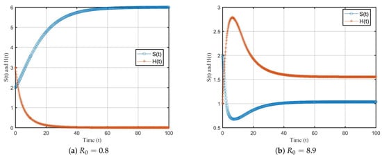
Figure 1. Evolution of susceptible S(t) and alcoholic H(t) with different $R_0$.

In Figure 2, we illustrate the effect of the transmission coefficient $\beta$ on the asymptotic behavior of the solution of the system. System parameters were chosen as follows: $\Lambda =0.8$, $\theta =0.1$, $\delta =0.1$, $\mu =0.1$, $\eta =0.1$, $d=0.2$, $h_1=10$, and $h_2=20$; $f^{\prime }\left(\sigma \right)$ and $g^{\prime }\left(\sigma \right)$ represent uniform distribution density functions, the initial conditions ${\phi }_1\left(\alpha \right)=2$, ${\phi }_2\left(\alpha \right)=1$ for $\alpha \in \left[-20,0\right]$. We chose eight different $\beta$ values. Figure 2 shows the evolution of susceptible $S\left(t\right)$ and alcoholic $H\left(t\right)$ with different $\beta$. Comparing the results, we can conclude that $\beta$ has a positive impact on the size of alcoholic $H\left(t\right)$ while negatively affecting the size of susceptible $S\left(t\right)$. Furthermore, $\beta$ has a notable influence on the types of equilibrium.

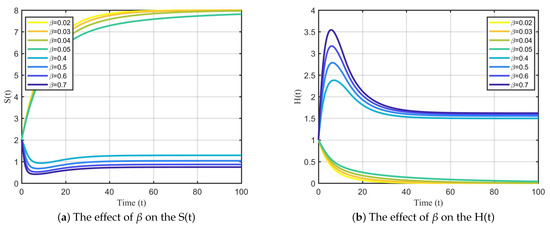
Figure 2. Evolution of susceptible S(t) and alcoholic H(t) with different $\beta$.

In Figure 3, we demonstrate the impact of $\delta$ on the asymptotic behavior of the solutions of the system. We chose the parameters as follows: $\Lambda =0.9$, $\beta =0.1$, $\theta =0.1$, $\mu =0.1$, $\eta =0.1$, $d=0.2$, $h_1=10$, and $h_2=20$; the initial conditions ${\phi }_1\left(\alpha \right)=2$, ${\phi }_2\left(\alpha \right)=1$ for $\alpha \in \left[-20,0\right]$. $f^{\prime }\left(\sigma \right)$ and $g^{\prime }\left(\sigma \right)$ represent uniform distribution density functions. Then, we selected eight different values of $\delta$. As shown in Figure 3, we find that an increase in $\delta$ negatively affects the size of alcoholic $H\left(t\right)$ and positively affects the size of susceptible $S\left(t\right)$, and it will also affect the final size of susceptible individuals and alcoholics.

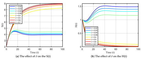
Figure 3. Evolution of susceptible S(t) and alcoholic H(t) with different $\delta$.

In Figure 4, we show the simulation of the evolution of susceptible $S\left(t\right)$ and alcoholic $H\left(t\right)$ under different initial conditions. $f^{\prime }\left(\sigma \right)$ and $g^{\prime }\left(\sigma \right)$ represent uniform distribution density functions. As shown in Figure 4a, we set the following parameters $\Lambda =0.6$, $\beta =0.05$, $\theta =0.1$, $\delta =0.1$, $\mu =0.1$, $\eta =0.1$, $d=0.2$, $h_1=7$, and $h_2=7$; the basic reproduction number was obtained as $R_0=0.83<1$. We chose four sets of initial value profiles ${\phi }_1\left(\alpha \right)$, ${\phi }_2\left(\alpha \right)$, for $\alpha \in \left[-20,0\right]$. We find that trajectories starting from different initial conditions tend to converge to the alcoholism-free equilibrium. In Figure 4b, we take the parameters $\Lambda =0.7$, $\beta =0.3$, $\theta =0.2$, $\delta =0.1$, $\mu =0.1$, $\eta =0.1$, $d=0.2$, $h_1=5$, and $h_2=5$. We calculated that $R_0=6.66>1$. We chose four sets of initial value profiles ${\phi }_1\left(\alpha \right)$, ${\phi }_2\left(\alpha \right)$, for $\alpha \in \left[-20,0\right]$. We observed that trajectories starting from different initial conditions tend to converge to the alcoholism equilibrium, which confirms our proof.

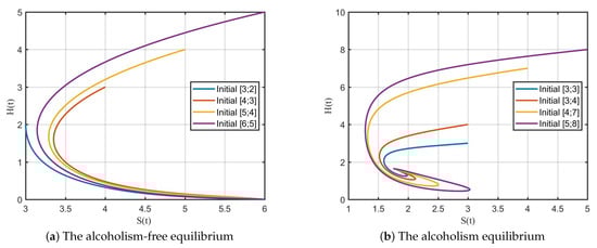
Figure 4. Phase portrait of S(t), H(t).

As shown in Figure 5, we simulated the impact of delays on the spread of alcoholism. We set the parameters in Figure 5a as follows: $\Lambda =0.8,\beta =0.3,\theta =0.1,\mu =0.1,$$\delta =0.1,\eta =0.1$, ${\phi }_1\left(\alpha \right)=2,{\phi }_2\left(\alpha \right)=3,\alpha \in [-h,0]$, and chose three sets of different delays $[h_1,h_2]$. The simulation results clearly showed that the latency period of alcoholism has a significant effect on the final scale of infection. The longer the latency period is, the smaller the scale of infection becomes. From Figure 5b, we selected the following parameters: $\Lambda =0.8,\beta =0.4,\theta =0.1,\mu =0.1,\delta =0.2,\eta =0.1,{\phi }_1\left(\alpha \right)=2,{\phi }_2\left(\alpha \right)=1,\alpha \in [-h,0]$ and chose three sets of different delays $[h_1,h_2]$. The simulation results showed that the duration of the relapse period of alcoholism also affects the scale of infection. The longer the relapse period is, the smaller the scale of infection becomes. However, the time delay does not significantly affect the rate of convergence of the curve. The numerical simulation results are in complete agreement with our theoretical analysis.

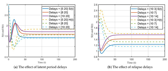
Figure 5. Evolution of susceptible S(t) and alcoholic H(t) with different delays.

7. Conclusions

In this paper, we considered the delay between a susceptible individual becoming an alcoholic and alcoholic relapse during treatment. We also incorporated saturation incidence into the model, leading to the development of an alcoholism epidemic model that includes distributed delays and relapse. The model was demonstrated to be well-posed. We then calculated the basic reproduction number $R_0$ using the next-generation approach. To understand the dynamics of this alcoholism epidemic model, we conducted a stability analysis of the equilibrium. This analysis revealed that, if $R_0<1$, the alcoholism-free equilibrium $P_0$ is locally asymptotically stable. Conversely, if $R_0>1$, the alcoholism equilibrium $P_{*}$ is locally asymptotically stable. Furthermore, by applying the Lyapunov function and LaSalle’s invariance principle, we obtained the global asymptotic stability of the equilibria. If $R_0<1$, the alcoholism-free equilibrium $P_0$ is globally asymptotically stable, whereas if $R_0>1$, the alcoholism equilibrium $P_{*}$ is globally asymptotically stable.

In order to analyze the influence of various parameters on the spread of alcoholism, we conducted a sensitivity analysis of $R_0$ with respect to $\beta$, $\delta$, $h_1$, and $h_2$. The analysis results indicated that reducing exposure to alcoholism is the most-effective method to control the spread of alcoholism. Simultaneously, increasing the treatment rate $\delta$ also effectively controls the spread. Interestingly, we found that extending the latency delay $h_1$ and relapse delay $h_2$ also effectively contributes to the control of the spread of alcoholism.

To support the comprehension of our theoretical findings, we designed several numerical experiments, the details of which are presented in Section 6. The results of the numerical simulation suggested that reducing the infection rate and increasing the treatment rate can help control the spread of alcoholism. Therefore, it is recommended to minimize contact with alcoholics and ensure that those with severe alcoholism receive treatment promptly. These measures can help to reduce the scale of alcoholism transmission. Furthermore, the simulations showed that the longer the incubation and relapse periods of alcoholism are, the smaller the scale of alcoholism. Thus, it is recommended that those in the latent stage of alcoholism avoid excessive alcohol consumption in a short period of time, and those who have recovered after treatment should avoid relapsing into excessive alcohol consumption in a short period. These measures can also contribute to the control of alcoholism.

References

- Petrakis, I.L.; Gonzalez, G.; Rosenheck, R.; Krystal, J.H. Comorbidity of alcoholism and psychiatric disorders: An overview. Alcohol Res. Health 2002, 26, 81. [Google Scholar]
- Sharma, S.; Samanta, G.P. Analysis of a drinking epidemic model. Int. J. Dyn. Control 2015, 3, 288–305. [Google Scholar] [CrossRef]
- World Health Organization. Global Status Report on Alcohol and Health 2018; World Health Organization: Geneva, Switzerland, 2019.
- Shield, K.D.; Parry, C.; Rehm, J. Chronic diseases and conditions related to alcohol use. Alcohol Res. Curr. Rev. 2014, 35, 155. [Google Scholar]
- Saunders, J.B.; Aasland, O.G.; Amundsen, A.; Grant, M. Alcohol consumption and related problems among primary health care patients: WHO collaborative project on early detection of persons with harmful alcohol consumption—I. Addiction 1993, 88, 349–362. [Google Scholar] [CrossRef] [PubMed]
- Rehm, J.; Gmel Sr, G.E.; Gmel, G.; Hasan, O.S.; Imtiaz, S.; Popova, S.; Probst, C.; Roerecke, M.; Room, R.; Samokhvalov, A.V.; et al. The relationship between different dimensions of alcohol use and the burden of disease—An update. Addiction 2017, 112, 968–1001. [Google Scholar] [CrossRef] [PubMed]
- Rehm, J.; Imtiaz, S. A narrative review of alcohol consumption as a risk factor for global burden of disease. Subst. Abus. Treat. Prev. Policy 2016, 11, 1–12. [Google Scholar] [CrossRef] [PubMed]
- Rocco, A.; Compare, D.; Angrisani, D.; Zamparelli, M.S.; Nardone, G. Alcoholic disease: Liver and beyond. World J. Gastroenterol. WJG 2014, 20, 14652. [Google Scholar] [CrossRef]
- Wechsler, H.; Lee, J.E.; Kuo, M.; Lee, H. College binge drinking in the 1990s: A continuing problem results of the Harvard School of Public Health 1999 College Alcohol Study. J. Am. Coll. Health 2000, 48, 199–210. [Google Scholar] [CrossRef]
- O’Malley, P.M.; Johnston, L.D. Epidemiology of alcohol and other drug use among American college students. J. Stud. Alcohol 2002, 14, 23–39. [Google Scholar] [CrossRef]
- Akmatov, M.K.; Mikolajczyk, R.T.; Meier, S. Alcohol consumption among university students in North Rhine–Westphalia, Germany—Results from a multicenter cross-sectional study. J. Am. Coll. Health 2011, 59, 620–626. [Google Scholar] [CrossRef]
- Benedict, B. Modeling alcoholism as a contagious disease: How infected drinking buddies spread problem drinking. SIAM News 2007, 40, 11–13. [Google Scholar]
- Mubayi, A.; Greenwood, P.E.; Castillo-Chavez, C.; Gruenewald, P.J.; Gorman, D.M. The impact of relative residence times on the distribution of heavy drinkers in highly distinct environments. Socio-Econ. Plan. Sci. 2010, 44, 45–56. [Google Scholar] [CrossRef] [PubMed]
- Mulone, G.; Straughan, B. Modeling binge drinking. Int. J. Biomath. 2012, 5, 1250005. [Google Scholar] [CrossRef]
- Huo, H.F.; Song, N.N. Global stability for a binge drinking model with two stages. Discret. Dyn. Nat. Soc. 2012, 2012, 829386. [Google Scholar] [CrossRef]
- Manthey, J.L.; Aidoo, A.Y.; Ward, K.Y. Campus drinking: An epidemiological model. J. Biol. Dyn. 2008, 2, 346–356. [Google Scholar] [CrossRef] [PubMed]
- Ma, S.H.; Huo, H.F.; Meng, X.Y. Modelling alcoholism as a contagious disease: A mathematical model with awareness programs and time delay. Discret. Dyn. Nat. Soc. 2015, 2015, 260195. [Google Scholar] [CrossRef]
- Bouajaji, R.; Abta, A.; Laarabi, H.; Rachik, M. Optimal control of a delayed alcoholism model with saturated treatment. Differ. Equations Dyn. Syst. 2021, 1–16. [Google Scholar] [CrossRef]
- Allsop, S.; Saunders, B.; Phillips, M. The process of relapse in severely dependent male problem drinkers. Addiction 2000, 95, 95–106. [Google Scholar] [CrossRef]
- Sharma, S.; Samanta, G.P. Drinking as an epidemic: A mathematical model with dynamic behaviour. J. Appl. Math. Inform. 2013, 31, 1–25. [Google Scholar] [CrossRef]
- Agrawal, A.; Tenguria, A.; Modi, G. Role of epidemic model to control drinking problem. Int. J. Sci. Res. Math. Stat. Sci. 2018, 5, 4. [Google Scholar] [CrossRef]
- Djillali, S.; Bentout, S.; Touaoula, T.M.; Tridane, A. Global dynamics of alcoholism epidemic model with distributed delays. Math. Biosci. Eng. 2021, 18, 8245–8256. [Google Scholar] [CrossRef] [PubMed]
- Den Driessche, P.V.; Watmough, J. Reproduction numbers and sub-threshold endemic equilibria for compartmental models of disease transmission. Math. Biosci. 2002, 180, 29–48. [Google Scholar] [CrossRef] [PubMed]
- Salle, J.P.L. The Stability of Dynamical Systems; Society for Industrial and Applied Mathematics: Philadelphia, PA, USA, 1976. [Google Scholar]
- Chitnis, N.; Hyman, J.M.; Cushing, J.M. Determining important parameters in the spread of malaria through the sensitivity analysis of a mathematical model. Bull. Math. Biol. 2008, 70, 1272–1296. [Google Scholar] [CrossRef] [PubMed]
Disclaimer/Publisher’s Note: The statements, opinions and data contained in all publications are solely those of the individual author(s) and contributor(s) and not of MDPI and/or the editor(s). MDPI and/or the editor(s) disclaim responsibility for any injury to people or property resulting from any ideas, methods, instructions or products referred to in the content. |
© 2023 by the authors. Licensee MDPI, Basel, Switzerland. This article is an open access article distributed under the terms and conditions of the Creative Commons Attribution (CC BY) license (https://creativecommons.org/licenses/by/4.0/).