Abstract
An important action-planning problem is considered for participants of the pursuit–evasion game with multiple pursuers and a high-speed evader. The objects of study are mobile robotic systems and specifically small unmanned aerial vehicles (UAVs). The problem is complicated by the presence of significant wind loads that affect the trajectory and motion strategies of the players. It is assumed that UAVs have limited computing resources, which involves the use of computationally fast and real-time heuristic approaches. A novel and rapidly developing intelligent–geometric theory is applied to address the discussed problem. To accurately calculate the points of the participant’s rapprochement, we use a geometric approach based on the construction of circles or spheres of Apollonius. Intelligent control methods are applied to synthesize complex motion strategies of participants. A method for quickly predicting the evader’s trajectory is proposed based on a two-layer neural network containing a new activation function of the “s-parabola” type. We consider a special backpropagation training scheme for the model under study. A simulation scheme has been developed and tested, which includes mathematical models of dynamic objects and wind loads. The conducted simulations on pursuit–evasion games in close to real conditions showed the prospects and expediency of the presented approach.
Keywords:
pursuit–evasion games; intelligent control; geometric control; unmanned aerial vehicle; path planning; trajectory tracking; trajectory prediction; machine learning; wind disturbances; modeling MSC:
68T20; 68T05; 49N75
1. Introduction
1.1. Motivation
Problems related to different pursuit–evasion games appeared in the early 1950s in the framework of game theory [1]. In the general case, the objective of the pursuers is to apply the behavior and action strategies that minimize the capture time while the evader tries to avoid being surrounded. Problem statements may be varied depending on the number of competitors, homogeneity and speed of the players (participants), level of information availability [2], model of the workspace (graph or geometric), or level of interaction (cooperative or non-cooperative) [3]. One of the first and most important applications of the results obtained in this field of science is the closely related theory of optimal control [4,5]. For the first time, the problem of pursuing a moving object with another controlled object was formulated as an optimal control problem in a paper [6]. The strategy of parallel pursuit was introduced in [7] and used to solve simple pursuit problems under phase constraints on the states of the players. A significant contribution to the theory of pursuit–evasion games based on the extremal aiming method was made in [8,9]. Paper [10] provides a methodology for designing strategies for players that guarantee either capture or evasion of all or some evaders in multi-player pursuit–evasion games when the players’ dynamics are represented by nonlinear models.
In mobile robotics, pursuit–evasion games are of great practical importance, with a wide range of applications, including environmental monitoring and surveillance [11]. They play a special role in search-and-rescue missions when the lost dynamic object or person as an adversarial entity tries to avoid being found [12]. Despite intensive research and advances in the theory of differential games, due to the active development of robotics and the increasing complexity of the tasks being solved, new actual challenges arise. One of them is solving problems under conditions of uncertainty when the external environment is unknown or unstable [13]. It is also known that modern algorithms dealing with differential games have a high computational complexity [14], which can cause difficulties in their implementation in small robotic systems. Often, the search for optimal mathematical solutions is replaced by the development of rational action strategies for players. For mobile robots, action strategies are often integrated with trajectory-tracking and obstacle-avoidance techniques [15]. One of the most challenging problems is to improve decision making autonomy both for individual mobile robots and their groups. Thus, for the successful implementation of pursuit–evasion strategies in mobile robotics, a number of urgent scientific problems need to be addressed.
1.2. Related Works
The main approaches to modeling the outcomes of pursuit–evasion games are based on cooperative [16] and non-cooperative [17] strategies, each with its own strengths and limitations. For non-cooperative strategies, the Nash equilibrium is usually taken as the main principle of optimality. Cooperative strategies impose additional conditions related to the ability to exchange full or partial information between participants. This approach poses new issues that involve the appointment of leaders and the decomposition of the team task [18]. At the same time, the decision-making process in cooperative games typically will require more time for calculations. Paper [19] proves the noteworthy fact that, in general, pursuers do not always benefit from cooperating as a team and that acting as non-cooperative players can lead to a higher probability of catching the evader. A research hotspot in pursuit–evasion games is to use formation-control strategies in the process of encircling the evader. Such strategies are aimed at avoiding collisions between pursuers, reducing the distance between each pursuer and the evader, and keeping the pursuers’ angular distribution [20]. The drawback is that rigid structures, especially when each agent is assigned to occupy a corresponding point in the formation, may reduce the efficiency of encirclement. A fundamental and still open question is to assess the advisability of using centralized (based on the knowledge of the full game state) or decentralized (based on the local information available to each player) approaches in a particular case. For certain problem statements, centralized strategies can be more beneficial [21], but in general, decentralized ones provide flexibility in decision making. In recent years, the self-organizing control approach has given robotic systems higher autonomy and robustness, so it is gradually and successfully used in intelligent control systems [22].
The choice of specific robotic systems as objects of study requires consideration of the corresponding exact mathematical models of their dynamics as well as restrictions on phase coordinates and control signals. Robotic systems are currently presented in wide variations, but in this work, the main objects of study are unmanned aerial vehicles (UAVs) as the convenient ground for testing the theory of differential games. Recently, there has been a growing trend toward the development of UAVs capable of carrying a payload and a significant expansion of their functionality [23]. Groups of UAVs that can operate in unstable environments are often used in firefighting [24], search and rescue [25], monitoring, and exploration missions [26]. In especially difficult conditions, the flight mission needs to be carried out with a partial lack of communication with the human operator or between members of the UAV group [27]. Therefore, one of the main challenges is to increase the autonomy of UAVs by developing algorithms for automatic trajectory and behavior planning [28]. At the same time, it should be noted that the necessary calculations must be performed in real-time and often under conditions of limited onboard computing resources. Real-time actions and timely decision making are needed, for example, to solve dynamic path planning [29], formation control [30], and pursuit–evasion problems. We note significant research [31] devoted to the collective behavior of robots when interaction is based on the use of a geometric acute angle test (AAT). Unlike the nearest-neighbor rule, the proposed approach allows for quickly checking the possibility of interactions with far neighbors and excludes unnecessary nearest neighbors. This paper proposes a controller to achieve collision-free coordination. As a result, a group of interacting agents has the advantages of scalability, effective coverage of areas, and reliability.
Research in the field of pursuit–evasion games involves studying the issue of adequately predicting the trajectory of a player with opposing interests. Current papers focus on the application of the following architectures: multilayer fully connected networks [32], recurrent neural networks in the form of long short-term memory (LSTM) [33,34], and gated recurrent units (GRUs) [35]. We note a comprehensive study on UAV trajectory prediction comparing five machine learning models [36]. Despite the obtained achievements, modern approaches to motion prediction do not always satisfy the limitations imposed on the computing power of onboard computers, while increasing autonomy requires the implementation of basic algorithms directly on board.
We note that one of the promising research areas is the application of game theory advances for solving trajectory problems in wind load conditions. A novel approach is that the UAV applies available strategies and tries to minimize the deviation from its reference pseudo-target that imitates an ideal trajectory of motion [37]. The authors of papers [38,39] apply the adapted theory of differential games for tracking aircraft trajectories under wind loads. The reference paths are obtained in an unperturbed environment as solutions to optimal control problems and tracked in the presence of severe wind disturbances. A special guide-based control procedure is introduced based on direct aiming to stabilize reference trajectories under unknown time-varying perturbations.
The objective from the evader’s point of view can be treated as a path-planning problem in the presence of dynamic obstacles [40], which becomes even more complicated in an environment with no-fly zones or additional static obstacles. We note that one of the most common approaches to solving the tasks of obstacle avoidance and pursuit–evasion is to use the potential fields method [41] and its various modifications [42]. The essence of the method is to implement the movement of a mobile robot using the forces of attraction to the target position and repulsion from obstacles. Another similar greedy strategy is proposed in [43], in which pursuers are attracted by the evader and rejected by other pursuers at the same time. A detailed review of the existing various general motion-planning and trajectory-tracking methods for UAVs is not given in the paper since it goes beyond the scope of this study. It is worth noting that the configuration of the workspace is of great importance; for example, [44] considers the problem of catching an evader in a closed convex domain. In the present research, we are dealing with an open, disturbed environment without additional objects.
So, we can summarize that the main challenges of the pursuit–evasion problem under study are the following:
- Integration of both optimal and heuristic algorithms within a single concept to improve decision efficiency under conditions of uncertainty;
- Creation of a comprehensive approach, including the development of behavioral strategies, mathematical models of players, and simulation under disturbances;
- Performing adequate linearization of differential equations describing the dynamics of UAVs and introducing other simplifications that do not lead to a significant loss of accuracy of the resulting solutions.
1.3. Main Contributions
Due to the computational complexity of solving differential games, one of the main trends is the integration of different approaches to model the most probable outcomes. Intelligent–geometric theory developed by the authors of the present work to control robotic systems under conditions of uncertainty is a new and promising area of research [45]. The basic idea is to combine the advantages of adaptive intelligent and precise geometric control [46] methods within a single robotic system. It is assumed that an intelligent control module should be used when the exact solution of the optimization problem cannot be found within given constraints—for example, under conditions of significant external uncertainty or in the case when prompt actions are required. Geometric control theory is aimed at solving the controllability problem, which implies finding a control function to transfer the initial state of the dynamic system to a prescribed state in finite time [47]. According to the theory, admissible trajectories and reachability sets formed by dynamic systems are related to the group of geometric transformations. In the present paper, we expand the study of intelligent–geometric control architecture and test it on the pursuit–evasion games between robotic systems. To model the outcomes of differential games within the framework of the geometric approach, we construct Apollonius circles, which are often used to create barrier boundaries for the evader [48].
To predict the evader’s trajectory, we introduce a training algorithm for a two-layer fully connected network with an activation function of the “s-parabola” type. The main advantage of the proposed model is its simple implementation, which corresponds to modern research in the field of accelerating the work of artificial neural networks (ANNs). For example, the new “s-parabola” function has an advantage over the sigmoid function in the speed of ANN training and prediction. Despite the recent achievements, to successfully implement pursuit–evasion strategies as well as modern path-planning methods in the onboard system of an aircraft, much more attention should be paid to modeling verisimilar external conditions, in particular severe windshear. Due to the limited computing resources of small autonomous aircraft, the problem of constructing intelligent and adaptive control algorithms remains a relevant issue.
In this research, we take advantage of drawing together intelligent and geometric control approaches under a unified architecture of a robotic system. We proposed a heuristic and fast evader’s strategy (which can be interpreted as a collision-avoidance algorithm) based on a modified potential field method and a geometric principle of Apollonius spheres construction. Also, the novelty of the study is to examine the goal-directed motion, when the evader needs not only to avoid the encirclement, but also to reach the target point. A model experiment of a goal-directed UAV flight under conditions of external disturbances and the presence of dynamic pursuers is carried out. To match the real conditions of the problem, the mathematical models of a small aircraft and wind disturbances are used. In addition, the problem of controlling the motion of a UAV along the given route in a perturbed environment is discussed and solved in accordance with the strategies that reflect the behavior of a human-operator and the principle of aiming at an object that imitates the ideal flight. The considered and studied approaches serve to achieve acceptable control accuracy by using simple tools that can be implemented in onboard control systems of small UAVs.
Thus, the authors’ contribution to solving this problem is as follows:
- The article describes the elements of the theory of intelligent–geometric control in relation to pursuit–evasion problems;
- Some game strategies have been developed for both the pursuer and the evader based on the solution of optimal problems and the application of heuristic rules;
- A model for predicting the movement of the evader is proposed, which expands the capabilities of the pursuer;
- Simulation of some game scenarios in a disturbed environment was carried out with the developed approaches.
- Subsequent sections are organized as follows:
- Section 2 contains problem statements for both the pursuer and the evader.
- Section 3 presents the architecture of intelligent–geometric control theory (Section 3.1), solutions to the optimization problem of the closest approach (Section 3.2 and Section 3.3), and heuristic strategies for players (Section 3.4). The problem of predicting the trajectory of the evader is considered in Section 3.5. The problem of moving along the required route given by waypoints is briefly described in Section 3.6.
- Section 4 is devoted to testing the proposed solutions. We first considered the planar case of the pursuit–evasion game in Section 4.1. Section 4.2 then discusses the dynamic model of an aircraft-type UAV and its linearization. Section 4.3 describes schemes for modeling the game in a disturbed environment for the spatial case. Simulation using the developed approach is carried out in Section 4.4.
- The final section, Section 5, contains the main conclusions and prospects for further research.
2. Problem Statement
When considering differential pursuit–evasion problems with several participants, there is a wide range of mathematical statements. One of the most practical and urgent challenges is the problem of one high-speed evader and several non-cooperative pursuers. In the research, we tried to address the game both in terms of pursuers and an evader. In the suggested problem statements and their solutions, the general three-dimensional case is established as a baseline, while the corresponding calculations for the two-dimensional case can be obtained in a similar way.
2.1. General Pursuit and Evasion Problems
We are dealing with a path-planning problem in which an evader should lay its route to a target point through the complex environment with dynamic obstacles (pursuers) . The pursuers are intelligent opponents that try to interfere with the mission and capture the evader. Further in the article, we consider kinematic (Section 2.2) and dynamic (Section 4.2) models of UAVs as objects of study. Let us introduce a fixed base coordinate system, where axis is directed upward relative to the terrestrial surface, axis is codirected with the projection of the longitudinal evader’s speed at the initial time instant, and axis is directed to the right. In the base coordinate system, we track the positions of the participants’ centers of mass. The orientation of each UAV is determined by the angles of pitch , yaw , and roll in a coordinate system fixed to the vehicle and having the origin at the center of mass. It is assumed that axes are parallel to the axes , and . For simplicity, the roll angle is discarded from subsequent calculations. Assume that variables related to an evader and pursuers are marked with the subscripts and , respectively. At time instant , participants and perform simple motion with speed ; angles of pitch ; and yaw . The states of pursuers and evader are described by the following vectors [45]:
where are coordinates that are assumed to be known at any arbitrary instant . It is supposed that the speed of evader is higher than the speed of any one of pursuer . As a result of wind action, vehicles can periodically severely deviate from their routes. In this case, UAVs are guided by a set of valid control strategies and rules, as well as the ability to control speed, pitch, and yaw angles, subject to the following restrictions:
Let and , respectively, denote the coordinates of players and . We consider the geometric model of a UAV as a sphere of radius to account for the safety margin. We designate the time when the evader reaches its target by and the time when one of the pursuers captures the evader by . From the evader’s point of view, the flight to its target should be safe, so it is assumed that the safety distance is determined as follows:
Evasion problem.
The motion-planning problem for a dynamic object on the time interval [0, Tg] under perturbations and constraints (2), (4) is to construct a control function such that:
where is the minimum desired distance between the evader and its target point .
The evasion task ends at time , when the meeting of the dynamic object with its target happens.
Pursuit problem.
For dynamic objects , the pursuit problem on the time interval [0, ] consists in synthesizing a control function under perturbations and constraints (3), such that:
where is the minimum needed distance between the pursuer and the evader.
The pursuit game is won at time when at least one of the pursuers approaches the evader (their coordinates become close enough), which is regarded as its capturing.
2.2. Optimal Convergence Problem
Let us consider the closest approach problem from the pursuer’s point of view on a local segment when it is needed to come as much closer as possible to the evader, given its predicted direction of motion. We are dealing with the motion of two aerial vehicles (pursuer and evader ) in ideal conditions without disturbances when the evader keeps its direction. The initial positions of players, direction , and speed of the evader are known. As it was proved in [49], until the evader changes its direction, the optimal pursuer strategy is to move in a straight line with maximum speed. So, it is supposed that the pursuer’s speed is assigned a value of ; velocity of the pursuer, velocity and orientation angles of the evader are constants. Let us assume that corresponds to the time of maximum convergence.
Optimal Convergence Problem.
The problem lies in constructing an optimal control function for the transition of system (1) with one pursuer
from the initial state to the final one while minimizing the distance between participants.
We introduce values , and give a mathematical description of the motion of aerial vehicles in an unperturbed environment. The simplified kinematic model of the pursuer’s motion is given by [49]:
The simplified kinematic model of the evader’s motion is given by
It is supposed that .
Let us introduce the following system:
Thus, we obtain the optimal control problem with restrictions (2) and (3):
Problem (10) can be solved using geometric control methods.
3. Materials and Methods
The solution of the formulated problems is based on the results obtained by the authors in the field of adaptive control of robotic systems, operating in turbulent and nondeterministic environments. The research relies on modern principles of intelligent, geometric, and automatic control of dynamic systems.
3.1. Intelligent–Geometric Control Architecture
Geometric control theory studies various approaches to differential geometric methods in dynamic systems control. The main objective of this relatively new area is to solve controllability and optimal control problems. The controllability problem resides in finding system states that are achievable from a given initial one. When all reachable states become known, it is necessary to find the best path in terms of the transition time, the length of the permissible trajectory, the energy expended, or the value of some other function. The search for such paths is the subject of the optimal control problem. The authors of [47] associate the use of the term “geometric” with the fact that the right side of an ordinary differential equation is a vector field, and the corresponding dynamic system is a flow generated by this field. Thus, the controlled system can be interpreted as a family of vector fields. It should also be noted that admissible trajectories and reachability sets are closely related to the group of transformations that form the foundations of geometry and are generated by the dynamic systems under study.
In the present research, the concept of geometric control is considered in a broad sense and includes the solution of various optimization problems associated with the path-planning and trajectory-tracking tasks. One of the most important ones is to calculate the direction of the pursuer for its closest possible approach to the target. If the capture is possible and the motion of the participants is piecewise linear, then the point of intersection can be calculated using Apollonius spheres. Another major issue is to follow the earlier obtained motion path presented by multiple reference points under disturbances and control restrictions while optimizing time and deviation. Problem statements from the field of automatic and geometric control complement each other, and at the same time, their solution requires detailed information about the nonlinear and complex system dynamics.
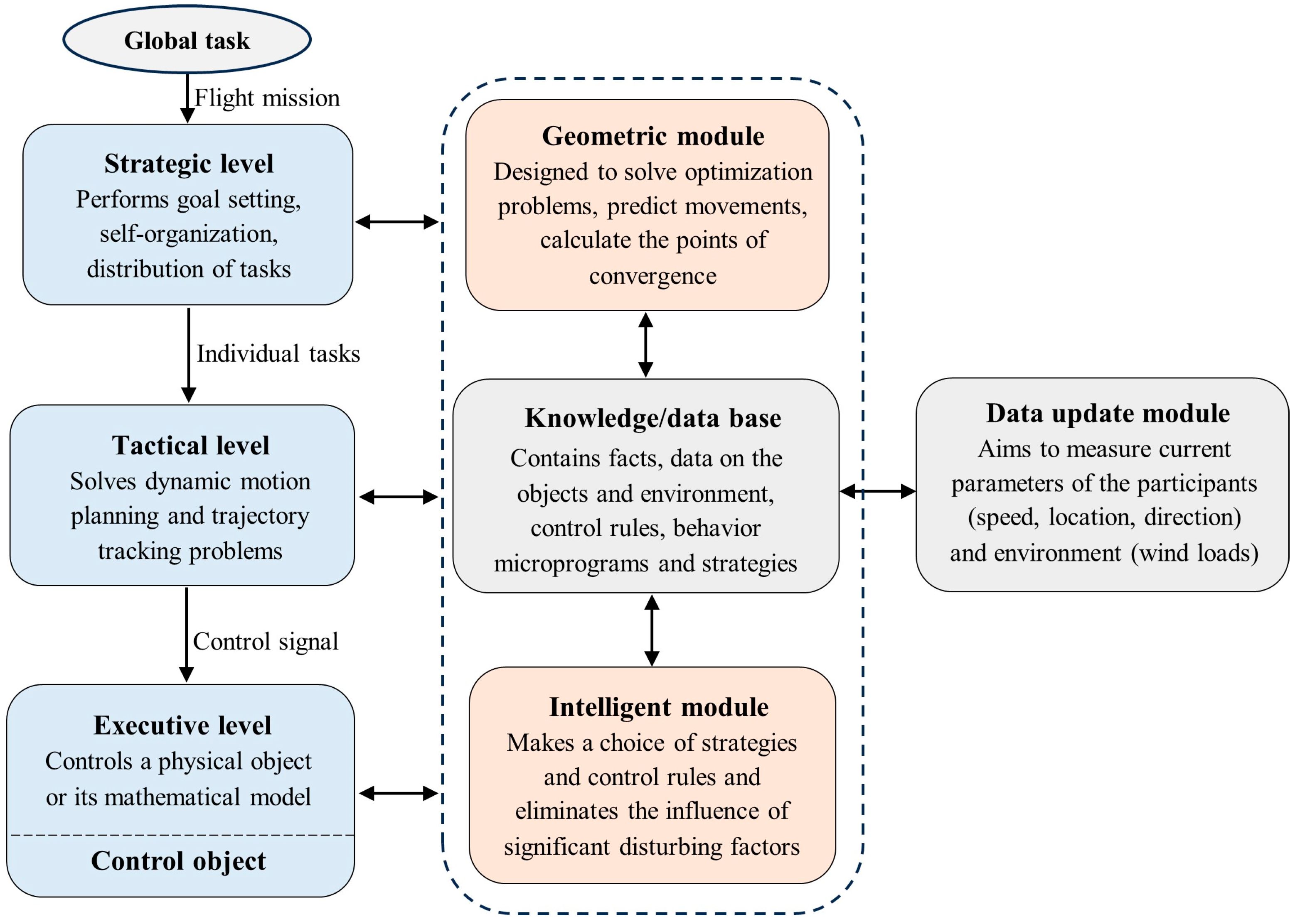
Increasing the autonomy of devices—for example, to make decisions in the absence of communication—often involves performing basic calculations on the onboard computer. The existing exact and approximate methods for solving optimal control problems are time-consuming, which can cause difficulties in their implementation in onboard computers with limited resources. The environmental instability, dynamic uncertainties, and external disturbances that influence the robotic systems can significantly complicate the decision-making process. Under such conditions, it will be expedient to develop a control architecture capable of supporting the tradeoff between accuracy and the required speed in making operational actions by rational combining accurate geometric and fast intelligent control methods [45]. The proposed three-level hierarchical scheme of intelligent–geometric control architecture is shown in Figure 1.
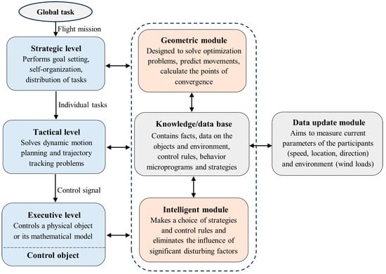
Figure 1.
Intelligent–geometric control architecture.
Unlike the intelligent–geometric control scheme presented in [45], Figure 1 more accurately reflects the structure of the system and the interaction between the main modules. In the general case, the strategic level serves to develop solutions to cooperative problems for a group of dynamic objects that can partially exchange information and know information about the state of the environment and their relative position. The main issues to be resolved are the distribution of roles and tasks, the choice of global strategies, and self-organization. As a result, individual tasks and strategies are formed for each object in a group, which are subsequently transferred to the tactical level. At the same time, in the present study, we assume that each pursuer acts independently, which makes this level unnecessary. The tactical level solves specific tasks of each dynamic object associated with static and dynamic motion planning in a complex, disturbed environment. After performing calculations, specific control signals are generated, which are later transferred for processing to the executive level. Each of these levels can rely in its calculations both on the geometric and intelligent control methods provided by the corresponding modules. The architecture includes an integrated module (knowledge/database) that contains information about the states of the environment and control objects, as well as contains ways to solve control problems in the form of rules and strategies.
3.2. Calculation of the Intercept Point
Let us consider a case when it is possible to accurately calculate the point of crossing the trajectory of a pursuer and an evader. Suppose that there is one pursuer and an evader with fixed velocity and direction of motion operating in an unperturbed environment. The initial coordinates and the speed of the considered participants are assumed to be known. Additionally, we suppose that angles of pitch and yaw of the evader are known. It is necessary to find the probable point of intersection ( and the direction of the pursuer’s motion.
The equation of a sphere, which is the locus of the participant’s convergence, is given as follows [37]:
Solving Equation (11) gives a pair of points that reflect the outcomes of the games in which an evader moves in opposite directions. Heading angles of pursuit can be calculated from the following equations:
Here, point corresponds to the single solution of Equation (11) with a certain fixed direction of the evader’s motion. Thus, the sphere of Apollonius shows the points of intersection for the pair of players with fixed velocities at various directions of motion, which can be used to develop action strategies.
3.3. Solution of the Optimal Convergence Problem
When the pursuer cannot calculate the exact intercept point with the evader (for example, the pursuer cannot catch up with the evader because of the lower speed), the optimization problem (10) arises in calculating the direction for the closest possible approach. To solve it, we apply the methods of geometric control, specifically Pontryagin’s maximum principle [50]. Let us introduce the following Hamiltonian:
where are functions of time and is a constant. We assume that and have
According to the conditions for the existence of an extremum of the function , we obtain:
Let us find :
From the transversality condition, we obtain:
To solve the problem, the following relations are used:
After the necessary simplifications, the following is derived:
From conditions (19) and (20), we can find flight parameters of the pursuer and the time of the closest approach to the target.
3.4. Pursuit and Evasion Strategies
In this section, based on the obtained results, the solution to the pursuit–evasion problem is addressed both from the point of view of the evader (5) and the pursuer (6). The present study improves and expands upon the players’ strategies discussed earlier in [37] and is a natural continuation of the authors’ research in this area. In general, participants of differential pursuit–evasion games are intelligent opponents with competing interests. The goal of the player is to assess its environment and calculate reasonable actions in a timely manner. Inspired by the potential fields method that is applied to the problem of obstacle avoidance [41] and the geometric approach involving the construction of Apollonius spheres, we proposed rational motion strategies. Consider the situation when there is one high-speed evader and a group of dynamic objects in the workspace. The states of all pursuers and an evader are assumed to be known at any given moment . We note that the initial position of the players and their maximum speed, in many cases, allow us to evaluate the possible outcome of the game.
3.4.1. Evader’s Strategy
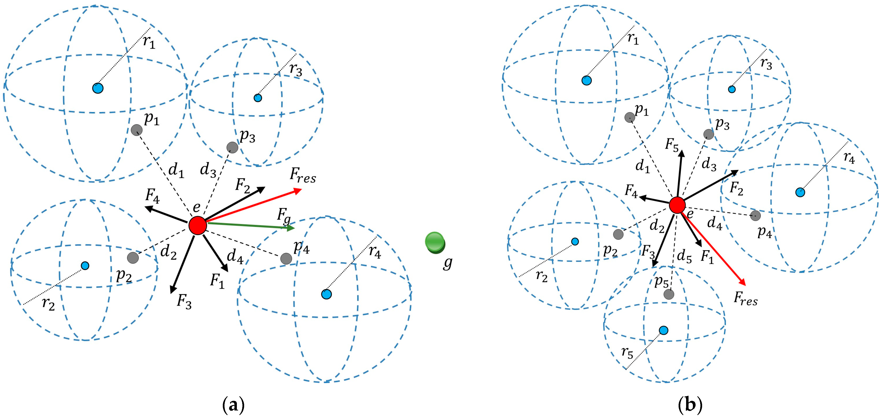
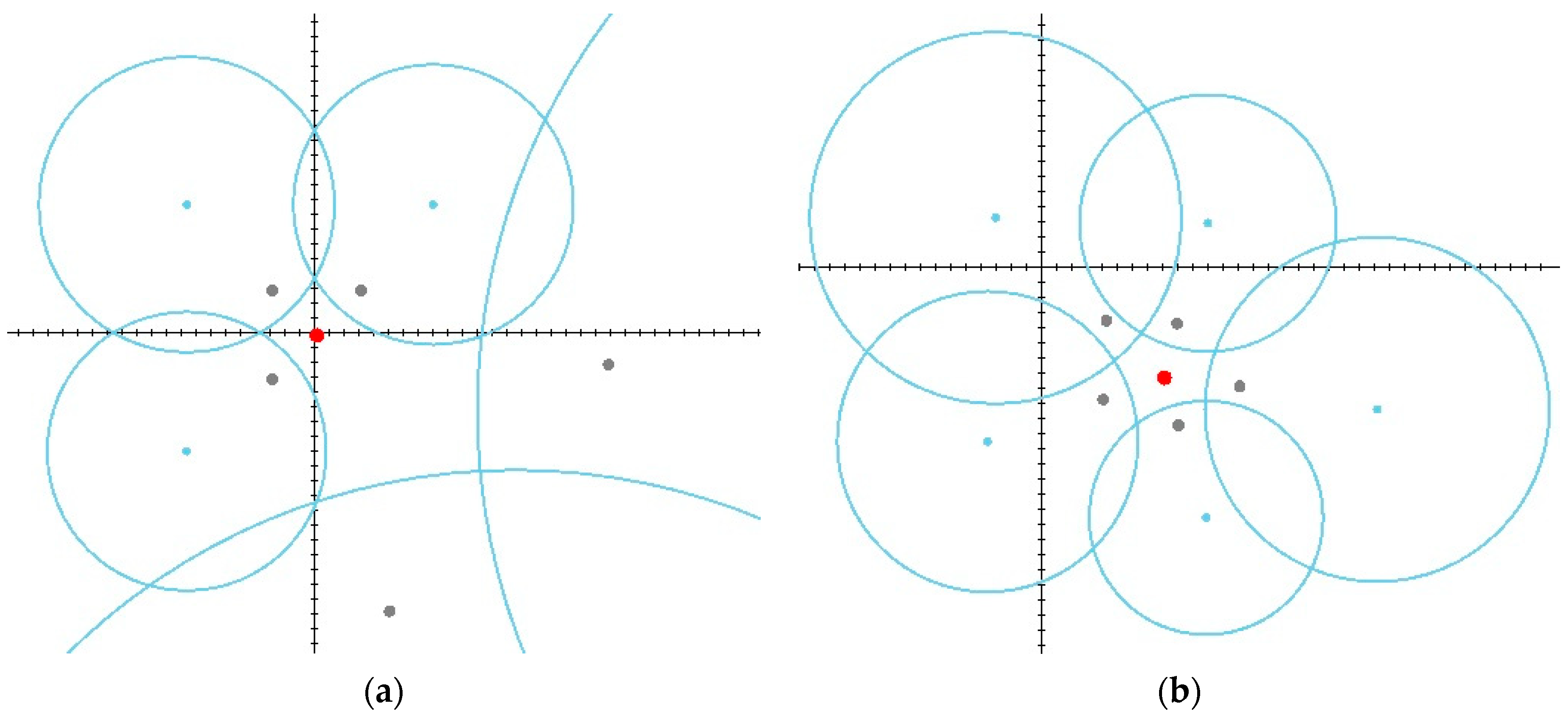
Let be the distance between objects and , while be the distance between target and object . It is reasonable to assume that the farther away a pursuer is, the less it should influence the evader’s motion strategy. We explore two variations of the game, in the first of which an evader needs to avoid collision with the pursuers and move to a safe distance, and in the second one, the evader additionally needs to reach the target point (the pursuers are not aware of the evader’s target point). The sum of vectors for the abovementioned cases is respectively defined as follows:
where are adjustable parameters; are unit vectors that start from evader’s location point and correspondingly coincide with the directions from to and from to , as shown in Figure 2a,b. Relation (21) determines the case when there is no target point [37], while relation (22) deals with the goal-directed flight.
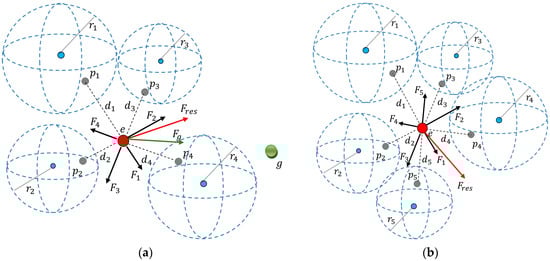
Figure 2.
Pursuit of an evader by a group of dynamic objects: (a) The evader’s movement is goal-directed; (b) There is no target point.
Figure 2 also shows the radii of Apollonius spheres for the corresponding pursuers . Below are the rational rules for the goal-directed flight of an evader, which differ from those proposed in [37] by taking into account the target point of the evader.
- If there are rays that do not intersect any of the Apollonius spheres, then choose the closest ray to the direction ;
- If exists, then the evader should move in this direction;
- If the ray cannot be calculated, then we suggest that the evader should move in the direction determined by vector (22).
The second option of the game has similar rules but excludes the target point . Vectors and are recalculated every time the state of participants or environment changes.
3.4.2. Pursuer’s Strategy
The objective of the pursuers is to surround the opponent through the creation of a special barrier formed by the spheres of Apollonius, which prevents its movement. We can give the following assessment of the possible outcome:
- If the evader is located in a closed region bounded by the spheres of Apollonius, it fails to escape;
- If it is possible to construct a half-line that does not intersect any of the spheres, then the evader manages to escape;
- In more complex cases—for instance, when the evader has a target point—to solve the problem, it is necessary to perform an accurate simulation of the game.
One of the possible rational strategies applicable to all uncoordinated pursuers could be the following:
- If the evader’s trajectory intersects with the corresponding sphere, then the pursuer must move to the point of convergence, which is calculated by Formulas (11) and (12);
- If the evader moves towards the Apollonius sphere but the exact intersection point cannot be calculated, it is necessary to move in the direction of the maximum approach, which is determined by Formulas (19) and (20);
- If the evader is moving away from the Apollonius sphere, then the pursuer must fly parallel to the evader by setting the appropriate direction. An alternative option is to build a forecast of the evader’s movement steps ahead, after which the pursuer begins to move to the calculated point , where is the current point in time and is the number of observed waypoints.
In contrast to the approach proposed in [37], the strategy of the pursuers was significantly improved by expanding the number of rules and incorporating Formulas (19) and (20), which allow for maintaining the integrity of the boundary formed by Apollonius spheres during the pursuit. In the presence of significant wind loads, the outcome of the game becomes even less predictable. Thus, in each specific case, it is necessary to model the game with the use of modern simulators in conditions close to real ones, suggesting that mathematical models of players and wind disturbances will be taken into account.
3.5. Neural Network Model for Predicting Evader’s Trajectory
The problem of constructing and training an artificial neural network model to quickly predict the opponent’s trajectory in pursuit–evasion games are solved. An original parabola-based activation function is used, which satisfies all the requirements for activation functions and has important new properties: it reduces the computational complexity of implementing nonlinearity and increases the efficiency of the ANN [51]. Unlike the previous study, which focused on the training of a neural network for basic logical functions, this paper proposes a general algorithm for training a two-layer neural network with an activation function of the “s-parabola” type. The considered activation function is a combined second-order curve using individual branches of a parabola, and in the general case, both branches can be used.
The upper branch of the parabola has the form ; that is, , while the lower branch of the parabola has the form , or .
Corresponding derivatives are as follows [51]:
- for :
- for :
Let us construct an s-shaped curve in which the upper part is the upper branch of the parabola, and the lower part reflects the lower part of the parabola relative to the ordinate axis. Thus, we obtain a composite s-shaped curve with an inflection point, which we will further call “s-parabola”. Figure 3 shows some variants of such a function for different values of .
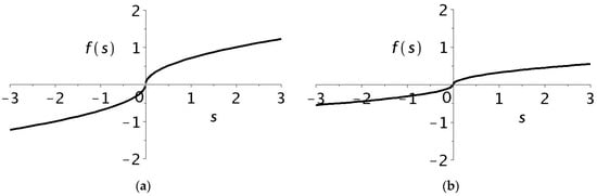
Figure 3.
Examples of s-shaped curves based on parabola branches for: (a) ; (b) .
Note that to solve a number of practical problems, it is sufficient to use only the first (upper) part of the s-shaped curves.
3.5.1. Algorithm for Training a Two-Layer ANN with the s-Parabola Activation Function
The training scheme with the specified activation function is common for tuning the parameters of an ANN using the backpropagation method, but it also has its own features. Let us consider, without loss of generality, an algorithm for training a feedforward ANN with inputs (), neurons in the first layer, two layers, and one output.
ANN training algorithm:
- Initialization of initial parameters and weights.
- Calculation of a neural network in the forward direction:
- Calculation of the first-layer signals:where , is the displacement of the parabola along the axis. The superscript for variables indicates the number of the neural network layer.
- Calculation of signals of the second (output) layer:
- Calculation of errors in inputs and outputs of neurons in the backward direction.
- Errors at the output and input of the last layer neuron.Output error: , where is the current value of the neuron output. The required value is set by the user. Error at neuron input: , where is the given input value of the second-layer neuron:
- Errors at the output and input of the th neuron of the first layer containing neurons.Errors in neuron outputs: where is the normalizing coefficient. On the other hand, , where , are the given and current output values of the th neuron of the first layer.Calculation of input signals for the activation function:Error at the input of the th neuron of the first layer: .
- Correction of the neural network weights, which is carried out as follows:where is the normalizing coefficient, is the learning rate, .
- If the error at the output is less than the predetermined value, then a stop is performed. Otherwise, the learning rate is reduced by a certain amount, , and the transition to step 2 is carried out.
3.5.2. An Example of Predicting the Planar Trajectory of an Evader
Let us assume that there is a time series of an evader’s positions observed during a certain time interval. We use the available values to predict its position at moment . We suppose that the number of observations is five (). Below, we propose a solution to the problem using an ANN with an s-parabola activation function.
The network consists of two layers. In the first layer, there are five neurons () with an activation function of the s-parabola type, given that , and , while in the second layer, there is one neuron of the same type. The number of inputs is equal to the number of neurons in the first layer (). The proposed network predicts the value of the next element of a time series based on the previous samples. The results of using the constructed neural network to predict the movement of the evader are presented in Figure 4.
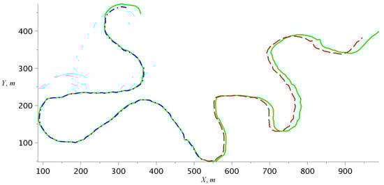
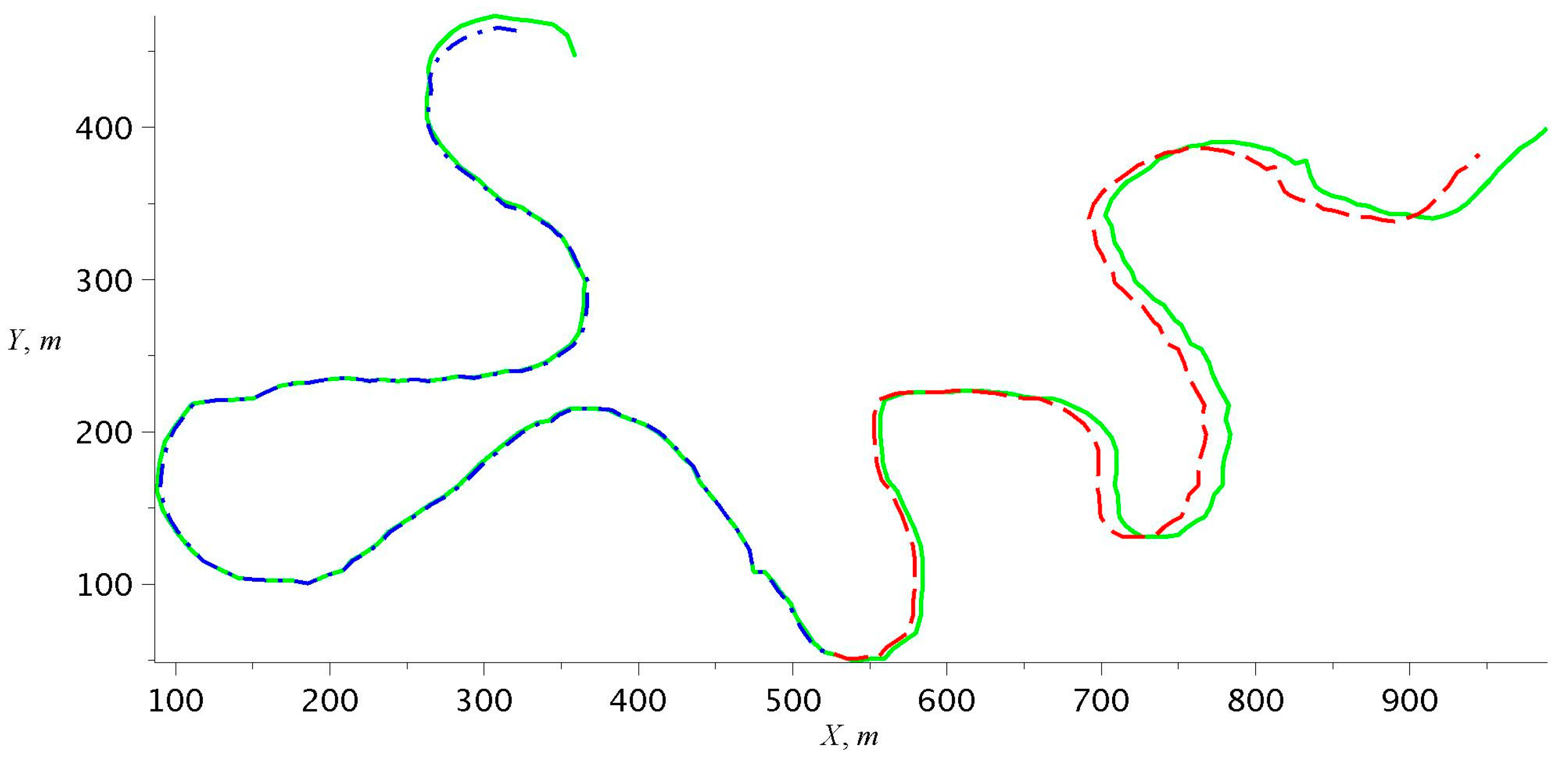
Figure 4.
The result of predicting the movement of the evader using a neural network with an activation function of the “s-parabola” type.
The solid green line in Figure 4 represents the participant’s actual trajectory. The prediction obtained on the training set is indicated by the dash-dotted blue line, and the results obtained on the test set are shown by the dashed red line. When training using x-coordinates, the average prediction error was 2.673, and the training time was 86.494 s. When training using y-coordinates, the average prediction error was 2.494, and the training time was 4.151 s.
3.6. Trajectory-Tracking Problem
One of the frequently encountered problems in robotics is to follow previously obtained routes with minimal deviations. Moreover, if the principal issue is to be at designated points of the path at certain times, then the problem of trajectory tracking arises. The exact formulation of such a problem for UAVs and its solution based on the pursuit–evasion theory were discussed by authors in earlier papers [37,45,49]. However, due to its urgency and gaining popularity, it is necessary to briefly discuss the issue based on the previously achieved results.
In the general case, intermediate reference waypoints of the route are known, through which the vehicle must fly at certain times . A novel approach is to introduce a pseudo-target that generates an ideal flight path. At the same time, the aircraft pursues its pseudo-target by controlling the speed and direction of flight. To approach the pseudo-target, we use a geometric approach that implies the calculation of the Apollonius sphere and the convergence point. In conditions of significant wind loads and uncertainty, it is advisable to apply intelligent control methods. An intelligent aerial vehicle may have a special knowledge base in which control rules are stored that define the conditions for generating control commands. Rational actions imitate the behavior of a human operator and are based on strategies implemented by sets of rules under given control restrictions and existing perturbations in accordance with the principles of dynamic systems modeling [52].
Let us briefly consider some control strategies to perform trajectory-tracking.
Strategy 1.
Point-by-point flight involves correcting the motion of a UAV in accordance with the current deviation from the given ideal trajectory. At that, all control points must be passed with a minimum deviation:
where is the moment of closest approach of the UAV to the control point .
Strategy 2.
The pursuit strategy involves calculating the speed, pitch, yaw, and appropriate point of the closest approach required for a UAV to capture its pseudo-target.
It is assumed that geometric invariants in the form of a sphere or an ellipsoid can be used to calculate the convergence point. In this case, the UAV does not need to pass exactly through all reference waypoints.
The developed strategies are integrated into a single control system designed to perform trajectory-tracking tasks under disturbances. Since these strategies are clearly described in earlier works, the detailed implementation here is omitted.
4. Results
A series of simulation studies of the pursuit–evasion game between dynamic objects has been carried out. The essence of the competition is that an evader tries to reach its target point in the shortest possible time, whereas the opponents, guided by their own strategies, are aiming to capture it. It is assumed that the velocity of the evader is greater than that of the pursuers.
4.1. Planar Case
First, for simplicity and convenience of visualization, the solution of the problem is studied in the yaw plane without detailed mathematical models of dynamic objects. To model the possible outcomes of the game, we use a special software developed in C# language (Microsoft Visual Studio Community 2022, version 17.6.5, Microsoft .NET SDK, version 4.8.09032, Microsoft, Redmond, WA, USA). For convenience of analysis, the results of three experiments involving different arrangements of players are visualized. Figure 5, Figure 6 and Figure 7 show the initial and final stages of the game while displaying the locations of the participants and the calculated circles of Apollonius. The target, evader, and pursuers are marked by green, red, and gray dots, respectively, whereas the Apollonius circles and their centers are marked by cyan.
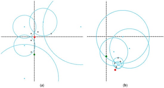
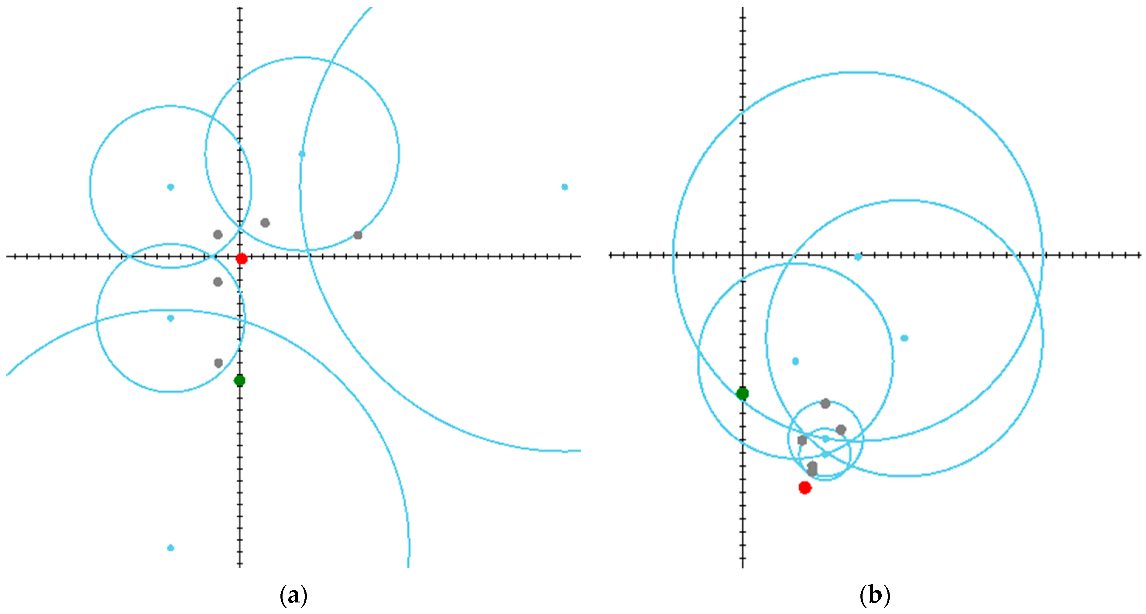
Figure 5.
Scenario in which an evader manages to escape but does not reach the target point: (a) The initial stage; (b) The final stage.
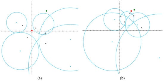
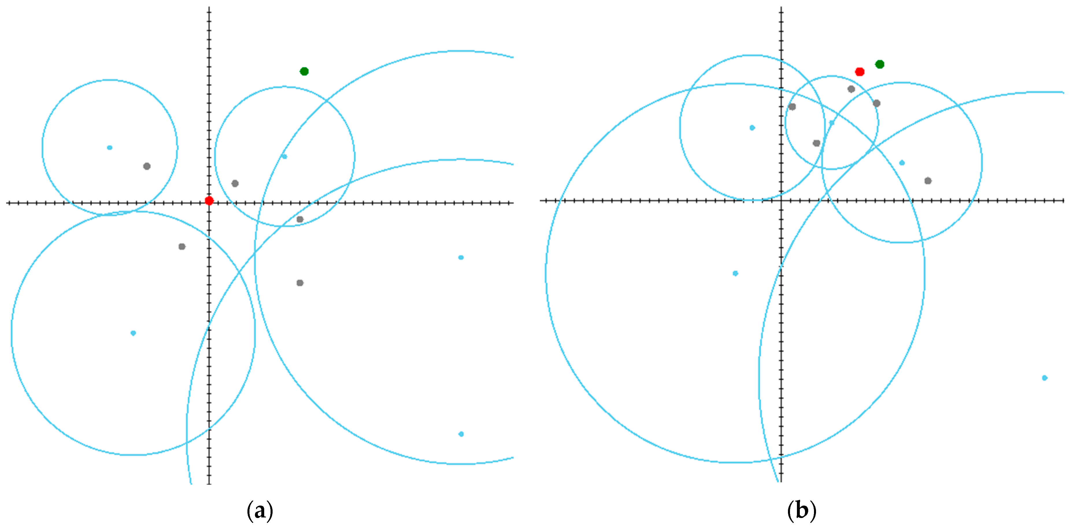
Figure 6.
Scenario in which an evader manages both to escape and reach the target point: (a) The initial stage; (b) The final stage.
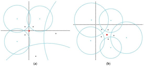
Figure 7.
Scenario in which an evader is surrounded by all pursuers: (a) The initial stage; (b) The final stage.
In the first scenario (Figure 5a,b), the runaway player manages to avoid capture, but the pursuers can stand on the way to the target point. As can be seen in the figure, if the evader initially tries to move directly towards the target, then it will be captured by one of the dynamic objects at the point of intersection of their paths, which lies on the corresponding circle of Apollonius. In this example, by using the proposed heuristic strategies and taking rational actions, the runaway escaped the encirclement but failed the mission to reach the target.
The second scenario (Figure 6a,b) assumes that, thanks to the favorable location of the target, the evader manages to both avoid its capture and complete the general task.
The last one (Figure 7a,b) deals with the case when the evaders’ only mission is to escape, but due to the specific players’ arrangement, it immediately becomes surrounded.
Table 1 below presents various outcomes of the game depending on the scenario, and the cells related to the participants indicate their coordinates and speed.

Table 1.
Outcomes of the pursuit–evasion game obtained from the new and previous strategies.
Some of the missions are only aimed at escaping the encirclement, while others additionally require the presence of a target point that must be reached.
Figure 5, Figure 6 and Figure 7 correspond to the cases shown in rows 1–3 in Table 1, respectively. Note that earlier in the authors’ works, the variant of the game where the pursuer needs to reach the target point was not considered [37]. The strategy of the pursuers has also been improved, now preventing gaps from appearing in the boundary formed by the Apollonius circles. The “Evader escapes” column in Table 1 shows whether the evader manages to escape in the corresponding scenario. Here, the first value shows the outcome of the game in accordance with the strategy described in this study, and the second one reflects the outcome of the game in accordance with the strategies from [37]. As can be seen in the table in scenarios 3 and 8, the improved strategy of the pursuers did not allow the evader to escape the encirclement.
The results obtained prove the feasibility of the proposed approach and its applicability in modeling pursuit–evasion games with one fast evader. The developed program is a tool for preliminary testing of various game scenarios and assessing the likelihood of each outcome.
4.2. UAV Dynamics Model
The equations of motion of a UAV (fixed-wing aircraft) in a turbulent atmosphere are considered in terms of the increments to the nonperturbed flight mode in the coordinate system fixed to the vehicle (the origin lies at the center of mass, the axis is directed along the longitudinal axis of the UAV, the axis is directed upward, and the axis is directed rightward).
We introduce the following notation:
- a, b, and c with various subscripts are the parameters of longitudinal dynamics depending on the UAV type and flight mode;
- k, l, and n with various subscripts are the parameters of lateral dynamics depending on the UAV type and flight mode;
- , , and are the pitch, yaw, and roll angles;
- is the elevator angle;
- , are deflection angles of the ailerons and rudder;
- , and are the projections of wind velocities on the , and axes of the base coordinate system;
- is the UAV speed relative to air in the unperturbed mode;
- are the projections of the UAV ground speed on the axes and ;
- , and are the coordinates of the center of mass on the , and axes;
- , and are the projections of the angular speed relative to air on the axes;
- is the correcting coefficient;
- is the Laplace transform parameter.
We make the following assumptions:
- The lateral and longitudinal motions are independent;
- The wind speed is significantly less than the speed of the UAV;
- The horizontal rectilinear flight under no wind conditions without roll and sliding is taken as the unperturbed mode.
In the unperturbed mode, the motion parameters have the following values (we use the subscript to mark the unperturbed mode):
The equations of the longitudinal motion in the restless atmosphere have the following form:
Here, denotes the deviation of values from their magnitude in the unperturbed mode. System (33) describes both short-period and long-period motions of the UAV. It can be simplified by going to the description in terms of short-period motions (the first and fourth equations and all terms with are excluded). This assumption is acceptable for most applied problems of flight dynamics. The simplified equations for the longitudinal motion in the restless atmosphere have the following form:
Since the pitch angle is measured in degrees, a correcting coefficient is introduced.
The equations of the lateral motion in the restless atmosphere have the following form:
Here, is the slip angle determined from the ground speed vector.
For the convenience of modeling dynamics, we will use the transfer functions from control and disturbing wind influences for the longitudinal and lateral movement of the UAV (fixed-wing aircraft) derived in [53].
For longitudinal dynamics, the resulting transfer functions from the control action of the elevator and wind components , to the pitch angular velocity are as follows:
For lateral dynamics, the resulting transfer functions from the control action of the rudder and the wind component to the yaw angular velocity have the following form:
Formulas (36) and (37) use the adjusted flight parameters of a small aircraft taken from [54]. The described transfer functions are further integrated into the structure of the flight-simulation scheme.
4.3. Matlab Simulation Scheme
The present section describes basic tools for conducting complex and full-fledged simulations of pursuit–evasion games under close-to-real conditions. We propose modeling schemes designed in a MATLAB/Simulink environment (version 8.4.0, MathWorks, Natick, MA, USA) in accordance with the principles of intelligent and geometric control theories.
The general control scheme for trajectory-tracking of a UAV presented in [45] is adapted to simulate the motion of both an evader (Figure 8a) and a pursuer (Figure 8b) in an unstable three-dimensional environment.
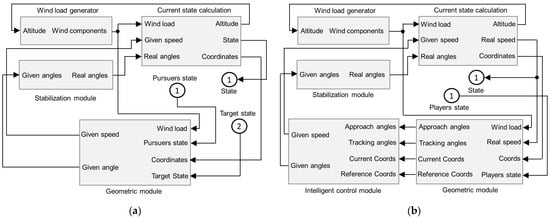
Figure 8.
General intelligent–geometric schemes for controlling the motion of dynamic objects: (a) For an evader; (b) For a pursuer.
The evader’s scheme contains the incoming coordinates of the pursuers and the target point. All necessary calculations in accordance with the strategy proposed in Section 3.4.1 are made in the geometric module.
The pursuer’s subsystem of intelligent–geometric control consists of two modules that complement each other. The geometric module is aimed at solving optimization problems of trajectory motion control with the given constraints [49] and accurate calculation of flight parameters. The intelligent control module is activated in unstable conditions to select among strategies (30) and (31) in accordance with the current situation. In accordance with the proposed scheme, the pursuer receives the coordinates of the evader and all closest obstacles (other pursuers). Intelligent and geometric blocks implement the pursuer’s strategy given in Section 3.4.2.
The “Current state calculation” block calculates the following UAV parameters: current position in the base coordinate system, current speed (taking into account wind load), and flight altitude. Wind loads are generated by the standard block “Wind Shear Model”.
To ensure the stability of the flight, we introduce a special “Stabilization module” that contains transfer functions (36) and (37) obtained from the equations of lateral and longitudinal motions of an aerial vehicle in a perturbed atmosphere. This block contains general control schemes for pitch and yaw angles and is discussed in detail in [49].
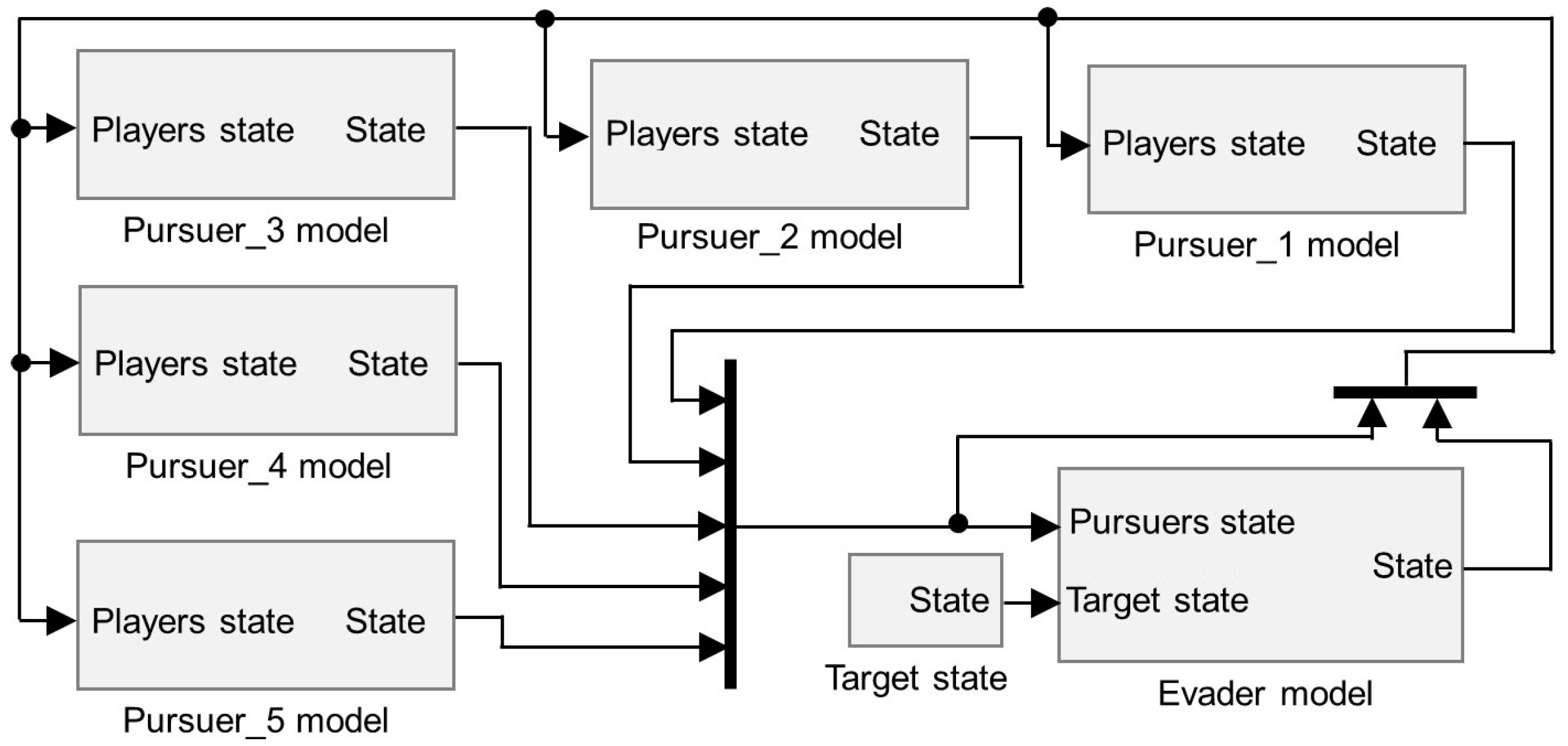
A general scheme is proposed for modeling a goal-directed flight of a UAV in the presence of dynamic obstacles that perform reasonable actions to capture it. As an example, Figure 9 shows a pursuit–evasion game for several (five) pursuers and one evader. This figure presents an updated version of the simulation scheme proposed in [37], taking into account the destination of the evader.
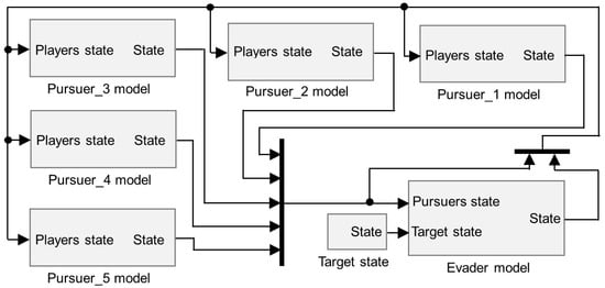
Figure 9.
The scheme of modeling the pursuit–evasion game with five pursuers and one evader.
The scheme includes the models of players’ dynamics and serves as the basis for solving complex motion control problems of aerial vehicles operating in an uncertain environment with obstacles.
4.4. Spatial Case
In accordance with the model proposed in the previous section (see Figure 9), simulation studies of the pursuit–evasion problem with five pursuers and one evader were carried out. The average airspeed of the pursuers was equal to 40 m/s, and that of the evader was 50 m/s. We take the rms values of the longitudinal and transversal components of the wind = 3 m/s.
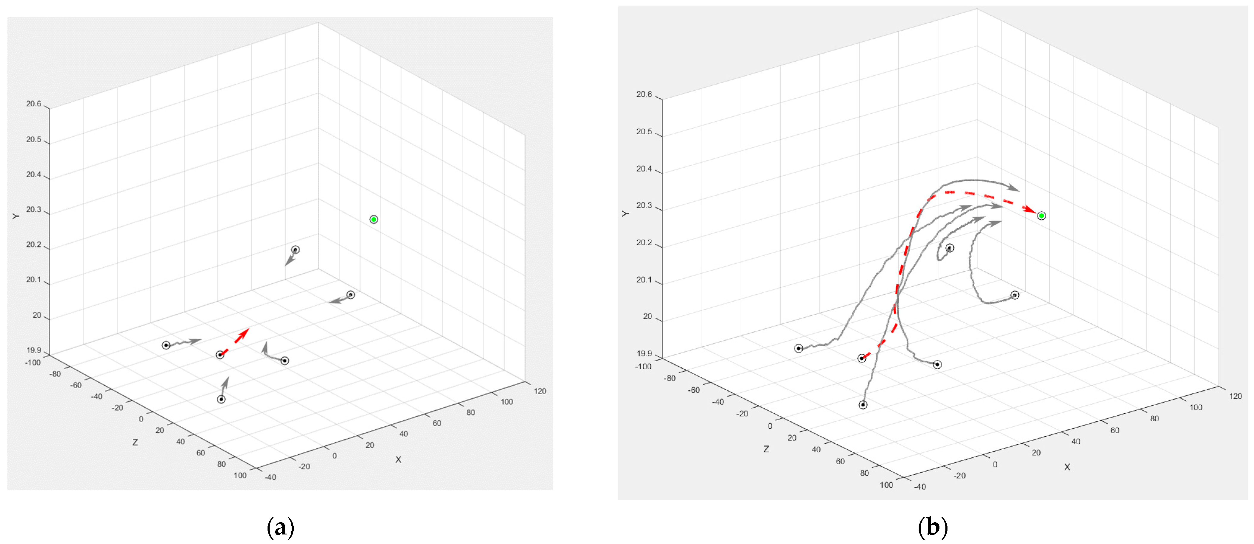
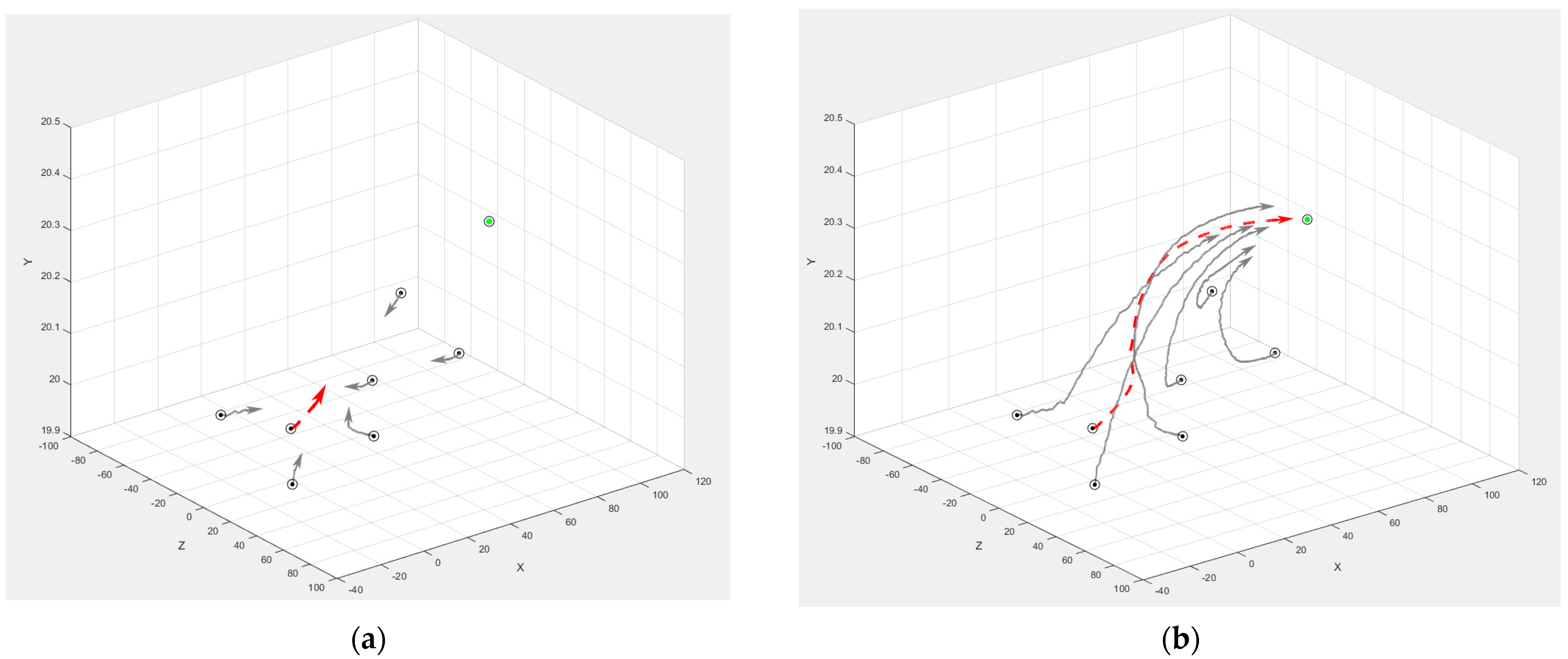
Figure 10 and Figure 11 show the results of the game with five and six pursuers, respectively. The spatial trajectories of the evader (dashed red curve) and dynamic obstacles (solid gray curves) were obtained in the MATLAB/Simulink environment. The initial positions of the players are marked with circles, and the target point is marked with a green dot. The arrows show the direction of movement of the players at the current moment. Figure 11 illustrates how adding another pursuer affects the evader’s trajectory.
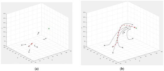
Figure 10.
Motion trajectories of the participants (for one evader and five pursuers): (a) At the initial stage; (b) At the final stage.
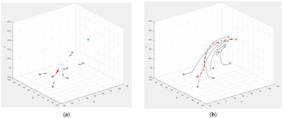
Figure 11.
Motion trajectories of the participants (for one evader and six pursuers): (a) At the initial stage; (b) At the final stage.
These examples illustrate the impact of wind loads on the flight route of the participants, performing logical actions to imitate the behavior of human operators. The figures also visualize how the proposed heuristic strategies form the trajectory of each player’s motion toward its target. We note that, in general, the proposed evader’s strategy increases the time to reach its target point but makes the flight safer. The developed methods and modeling system make it possible to test complex scenarios of the pursuit–evasion game in the presence of disturbances that affect the strategies of the participants.
5. Discussion
In this paper, we consider an approach to solving the problem of goal-directed motion planning for an unmanned aerial vehicle in the presence of dynamic obstacles and wind disturbances based on the use of pursuit–evasion strategies.
The main contributions of the study are as follows:
- For both the pursuers and the evader, we propose simple but effective heuristic rules that imitate the reasonable actions of a human operator in accordance with precise geometric calculations and the modified potential field approach.
- The problem of predicting the movement of an evader using a two-layer, fully connected feed-forward network is considered. A distinctive feature of the model is the use of a special activation function, which reduces the calculation time in conditions of limited computing power and the need to take prompt action.
- The solution of the trajectory tracking problem based on the principles of functioning of intelligent dynamic systems is discussed.
- A scheme for simulating pursuit–evasion games is proposed and studied that takes into account the dynamic models of participants and wind disturbances. A series of simulations conducted in MATLAB/Simulink environment demonstrates that the proposed strategies determine the natural behavior of dynamic objects under uncertainty.
We believe that the considered algorithms are advisable to use in control systems of small UAVs with limited computing resources. The obtained results sufficiently demonstrate the efficiency of the combined use of intelligent–geometric control approaches.
Future research will address the following important issues:
- Pursuers can be considered as intelligent agents, endowed with the ability to exchange information and make collective decisions. This approach determines the need to conduct research at the strategic level, related to issues of goal setting and distribution of tasks between participants.
- The problem statement can be expanded, for example, by considering scenarios with the low-speed agile evader or where the pursuers know the evader’s target point.
- Further improvement of the intelligent component is seen in the introduction of a knowledge representation model for describing the workspace in the form of semantic networks and the creation of appropriate decision-making procedures, increasing the intelligence of the participants themselves through the development of goal-setting approaches. This, of course, will require the creation of new strategies and algorithms.
- Finally, natural experiments are needed to demonstrate in practice the effectiveness of the developed intelligent–geometric control algorithms.
Flight control of the UAV is planned to be carried out using specialized software developed in high-level Java (version Java SE 19, Oracle, Austin, TX, USA) and Python (version 3.12.0, Python Software Foundation, Wilmington, DE, USA) languages. This includes a multimodal control command system and a multi-window simulator. All control software is distributed between the ground control station and the onboard computer system.
Author Contributions
Conceptualization, V.K. and M.K.; methodology, V.K.; software, M.K.; validation, M.K.; formal analysis, V.K.; investigation, V.K. and M.K.; resources, V.K. and M.K.; data curation, M.K.; writing—original draft preparation, M.K.; writing—review and editing, V.K. and M.K.; visualization, M.K.; supervision, V.K.; project administration, M.K.; funding acquisition, M.K. All authors have read and agreed to the published version of the manuscript.
Funding
This research was funded by RUSSIAN SCIENCE FOUNDATION, grant number 21-71-10056 (https://rscf.ru/en/project/21-71-10056/, accessed on 24 November 2023).
Data Availability Statement
The data presented in this study are available on request from the corresponding author.
Conflicts of Interest
The authors declare no conflict of interest.
Nomenclature
| Symbol Name | Definition |
| Axes of the base coordinate system | |
| Axes of the coordinate system fixed to the vehicle, and parallel to axes , and . | |
| Axes of the coordinate system fixed to the vehicle (the axis is directed along the longitudinal axis, the axis is directed upward, and the axis is directed rightward). | |
| Evader. | |
| th pursuer in group . | |
| Coordinates of the evader. | |
| Coordinates of the pursuer . | |
| Speed of the evader. | |
| Speed of the pursuer . | |
| Pitch and yaw angles of the evader. | |
| Pitch and yaw angles of the pursuer . | |
| Target point of the evader. | |
| Time moment when the evader reaches its target. | |
| Time moment when at least one of the pursuers captures the evader. | |
| Required distance between the evader and its target point. | |
| Radius of the geometric model of a UAV. | |
| Pitch, yaw, and roll angles. | |
| State of pursuer (coordinates and velocity). | |
| State of the evader (coordinates and velocity). | |
| Distance between objects . | |
| Unit vector that starts from evader’s location point and coincides with the direction from to . | |
| Unit vector that starts from evader’s location point and coincides with the direction from to . | |
| Ray that does not intersect any of the Apollonius spheres. | |
| , | Parameters of longitudinal dynamics. |
| Parameters of lateral dynamics. | |
| Elevator angle. | |
| , | Deflection angles of the ailerons and rudder. |
| Coordinates of the center of mass on the , axes. | |
| UAV airspeed. | |
| UAV speed relative to air in the unperturbed mode. | |
| Projections of the UAV ground speed on the axis . | |
| Projections of the angular speed on the axes. | |
| Laplace transform parameter. | |
| Transfer function from the control action of the elevator to the pitch angular velocity . | |
| Transfer functions from the wind components and to the pitch angular velocity . | |
| Transfer function from the control action of the rudder to the yaw angular velocity . | |
| Transfer function from the wind component to the yaw angular velocity . | |
| Reference time moment corresponding to the passage of the point by the UAV. | |
| Moment of closest approach of the UAV to the waypoint . | |
| Intermediate reference waypoint of the route. | |
| Coordinates of the UAV at time . | |
| Pseudo-target that simulates an ideal flight path. | |
| β | Displacement of the parabola along the axis. |
| Sum of weighted inputs on the th neuron of the first/second layer. | |
| Output signal of the th neuron of the first/second layer. | |
| Weight of the connection between the th input value and the th neuron of the first layer. | |
| Neural network output. | |
| Error at the output/input of the second layer. | |
| Error at the output/input of the th neuron of the first layer. | |
| Subscript indicates the target values of the corresponding parameters . |
References
- Isaacs, R. Differential Games: A Mathematical Theory with Applications to Warfare and Pursuit, Control and Optimization; Dover Publications: Mineola, NY, USA, 1999; ISBN 978-0-486-40682-4. [Google Scholar]
- Yang, B.; Liu, P.; Feng, J.; Li, S. Two-Stage Pursuit Strategy for Incomplete-Information Impulsive Space Pursuit-Evasion Mission Using Reinforcement Learning. Aerospace 2021, 8, 299. [Google Scholar] [CrossRef]
- Weintraub, I.E.; Pachter, M.; Garcia, E. An Introduction to Pursuit-Evasion Differential Games. In Proceedings of the 2020 American Control Conference (ACC), Denver, CO, USA, 1–3 July 2020; IEEE: Piscataway, NJ, USA, 2020; pp. 1049–1066. [Google Scholar] [CrossRef]
- Pesch, H.J. Solving Optimal Control and Pursuit-Evasion Game Problems of High Complexity. In Computational Optimal Control; Bulirsch, R., Kraft, D., Eds.; Birkhäuser: Basel, Switzerland, 1994; pp. 43–61. ISBN 978-3-7643-5015-4. [Google Scholar]
- Wang, Z.; Gong, B.; Yuan, Y.; Ding, X. Incomplete Information Pursuit-Evasion Game Control for a Space Non-Cooperative Target. Aerospace 2021, 8, 211. [Google Scholar] [CrossRef]
- Pontryagin, L.S.; Boltyanskij, V.G.; Gamkrelidze, R.V.; Mishchenko, E.F. The Mathematical Theory of Optimal Processes; Pergamon: Oxford, UK, 1964. [Google Scholar]
- Petrosjan, L.A. Differential Games of Pursuit; World Scientific: Singapore, 1993; ISBN 978-981-02-0979-7. [Google Scholar]
- Krasovskii, N.N.; Subbotin, A.I. Game-Theoretical Control Problems; Springer: New York, NY, USA, 1988. [Google Scholar]
- Subbotin, A.I. Generalized Solutions of First Order PDEs: The Dynamical Optimization Perspective; System & Control: Foundations & Applications; Birkhäuser Boston: Boston, MA, USA, 1995; ISBN 978-1-4612-6920-5. [Google Scholar]
- Stipanović, D.M.; Melikyan, A.; Hovakimyan, N. Guaranteed Strategies for Nonlinear Multi-Player Pursuit-Evasion Games. Int. Game Theory Rev. 2010, 12, 1–17. [Google Scholar] [CrossRef]
- Li, Y.; Liu, M.; Luan, P.; Zhou, J. Game Theory Methods for Pursuit-Evasion Problems. J. Phys. Conf. Ser. 2022, 2402, 012024. [Google Scholar] [CrossRef]
- Chung, T.H.; Hollinger, G.A.; Isler, V. Search and Pursuit-Evasion in Mobile Robotics: A Survey. Auton. Robot. 2011, 31, 299–316. [Google Scholar] [CrossRef]
- Zhang, L.; Prorok, A.; Bhattacharya, S. Pursuer Assignment and Control Strategies in Multi-Agent Pursuit-Evasion Under Uncertainties. Front. Robot. AI 2021, 8, 691637. [Google Scholar] [CrossRef]
- Borie, R.; Tovey, C.; Koenig, S. Algorithms and Complexity Results for Graph-Based Pursuit Evasion. Auton. Robot. 2011, 31, 317–332. [Google Scholar] [CrossRef]
- Sani, M.; Robu, B.; Hably, A. Pursuit-Evasion Game for Nonholonomic Mobile Robots with Obstacle Avoidance Using NMPC. In Proceedings of the 2020 28th Mediterranean Conference on Control and Automation (MED), Saint-Raphaël, France, 15–18 September 2020; IEEE: Piscataway, NJ, USA, 2020; pp. 978–983. [Google Scholar] [CrossRef]
- Han, L.; Song, W.; Yang, T.; Tian, Z.; Yu, X.; An, X. Cooperative Decisions of a Multi-Agent System for the Target-Pursuit Problem in Manned–Unmanned Environment. Electronics 2023, 12, 3630. [Google Scholar] [CrossRef]
- Sani, M.; Robu, B.; Hably, A. Pursuit-Evasion Games Based on Game-Theoretic and Model Predictive Control Algorithms. In Proceedings of the 2021 International Conference on Control, Automation and Diagnosis (ICCAD), Grenoble, France, 3–5 November 2021; IEEE: Piscataway, NJ, USA, 2021; pp. 1–6. [Google Scholar] [CrossRef]
- Zhu, Z.-Y.; Liu, C.-L. A Novel Method Combining Leader-Following Control and Reinforcement Learning for Pursuit Evasion Games of Multi-Agent Systems. In Proceedings of the 2020 16th International Conference on Control, Automation, Robotics and Vision (ICARCV), Shenzhen, China, 13–15 December 2020; IEEE: Piscataway, NJ, USA, 2020; pp. 166–171. [Google Scholar] [CrossRef]
- Talebi, S.; Simaan, M.A.; Qu, Z. Cooperative, Non-Cooperative and Greedy Pursuers Strategies in Multi-Player Pursuit-Evasion Games. In Proceedings of the 2017 IEEE Conference on Control Technology and Applications (CCTA), Mauna Lani Resort, HI, USA, 27–30 August 2017; IEEE: Piscataway, NJ, USA, 2017; pp. 2049–2056. [Google Scholar]
- Wang, X.; Cruz, J.B., Jr.; Chen, G.; Pham, K.; Blasch, E. Formation Control in Multi-Player Pursuit Evasion Game with Superior Evaders. In Defense Transformation and Net-Centric Systems; Suresh, R., Ed.; SPIE: Orlando, FL, USA, 2007; p. 657811. [Google Scholar]
- Casini, M.; Garulli, A. On the Advantage of Centralized Strategies in the Three-Pursuer Single-Evader Game. Syst. Control Lett. 2022, 160, 105122. [Google Scholar] [CrossRef]
- Liang, X.; Qu, X.; Wang, N.; Li, Y.; Zhang, R. A Novel Distributed and Self-Organized Swarm Control Framework for Underactuated Unmanned Marine Vehicles. IEEE Access 2019, 7, 112703–112712. [Google Scholar] [CrossRef]
- Nandwana, H.; Kashyap, V.; Chechani, A.; Saraswat, P.; Vijayvargiya, A. Design Analysis of Payload Carrying Quadcopter Using Finite Element Analysis. In Proceedings of the 2021 Smart Technologies, Communication and Robotics (STCR), Sathyamangalam, India, 9–10 October 2021; IEEE: Piscataway, NJ, USA, 2021; pp. 1–5. [Google Scholar]
- Akhloufi, M.A.; Couturier, A.; Castro, N.A. Unmanned Aerial Vehicles for Wildland Fires: Sensing, Perception, Cooperation and Assistance. Drones 2021, 5, 15. [Google Scholar] [CrossRef]
- Immanuel Damanik, J.A.; Dermawan Sitanggang, I.M.; Hutabarat, F.S.; Boy Knight, G.P.; Sagala, A. Quadcopter Unmanned Aerial Vehicle (UAV) Design for Search and Rescue (SAR). In Proceedings of the 2022 IEEE International Conference of Computer Science and Information Technology, Laguboti, North Sumatra, Indonesia, 19–21 October 2022; IEEE: Piscataway, NJ, USA, 2022; pp. 1–6. [Google Scholar]
- Yao, H.; Qin, R.; Chen, X. Unmanned Aerial Vehicle for Remote Sensing Applications—A Review. Remote Sens. 2019, 11, 1443. [Google Scholar] [CrossRef]
- Cesare, K.; Skeele, R.; Yoo, S.-H.; Zhang, Y.; Hollinger, G. Multi-UAV Exploration with Limited Communication and Battery. In Proceedings of the 2015 IEEE International Conference on Robotics and Automation (ICRA), Seattle, WA, USA, 26–30 May 2015; IEEE: Piscataway, NJ, USA, 2015; pp. 2230–2235. [Google Scholar]
- Ramesh, A.; Suseendhar, P.; Venugopal, E.; Sivakumar, P. An Overview of Navigation Algorithms for Unmanned Aerial Vehicle. In Proceedings of the 2023 International Conference on Intelligent Data Communication Technologies and Internet of Things (IDCIoT), Bengaluru, India, 5–7 January 2023; IEEE: Piscataway, NJ, USA, 2023; pp. 724–727. [Google Scholar]
- Gottlieb, Y.; Shima, T. UAVs Task and Motion Planning in the Presence of Obstacles and Prioritized Targets. Sensors 2015, 15, 29734–29764. [Google Scholar] [CrossRef]
- Chen, Q.; Jin, Y.; Wang, T.; Wang, Y.; Yan, T.; Long, Y. UAV Formation Control Under Communication Constraints Based on Distributed Model Predictive Control. IEEE Access 2022, 10, 126494–126507. [Google Scholar] [CrossRef]
- Ning, B.; Han, Q.-L.; Zuo, Z.; Jin, J.; Zheng, J. Collective Behaviors of Mobile Robots Beyond the Nearest Neighbor Rules with Switching Topology. IEEE Trans. Cybern. 2018, 48, 1577–1590. [Google Scholar] [CrossRef]
- Xue, M. UAV Trajectory Modeling Using Neural Networks. In Proceedings of the 17th AIAA Aviation Technology, Integration, and Operations Conference, Denver, CO, USA, 5–9 June 2017; American Institute of Aeronautics and Astronautics: Reston, VA, USA, 2017. [Google Scholar]
- Zhang, Y.; Jia, Z.; Dong, C.; Liu, Y.; Zhang, L.; Wu, Q. Recurrent LSTM-Based UAV Trajectory Prediction with ADS-B Information. In Proceedings of the GLOBECOM 2022—2022 IEEE Global Communications Conference, Rio de Janeiro, Brazil, 4–8 December 2022; IEEE: Piscataway, NJ, USA, 2022; pp. 1–6. [Google Scholar]
- Chen, S.; Chen, B.; Shu, P.; Wang, Z.; Chen, C. Real-Time Unmanned Aerial Vehicle Flight Path Prediction Using a Bi-Directional Long Short-Term Memory Network with Error Compensation. J. Comput. Des. Eng. 2023, 10, 16–35. [Google Scholar] [CrossRef]
- Yang, Z.; Tang, R.; Bao, J.; Lu, J.; Zhang, Z. A Real-Time Trajectory Prediction Method of Small-Scale Quadrotors Based on GPS Data and Neural Network. Sensors 2020, 20, 7061. [Google Scholar] [CrossRef]
- Peng, F.; Zheng, L.; Duan, Z.; Xia, Y. Multi-Objective Multi-Learner Robot Trajectory Prediction Method for IoT Mobile Robot Systems. Electronics 2022, 11, 2094. [Google Scholar] [CrossRef]
- Khachumov, M.V. Solution of the Problem of Group Pursuit of a Target Under Perturbations (Spatial Case). Sci. Tech. Inf. Process. 2018, 45, 435–443. [Google Scholar] [CrossRef]
- Botkin, N.; Turova, V.; Hosseini, B.; Diepolder, J.; Holzapfel, F. Tracking Aircraft Trajectories in the Presence of Wind Disturbances. Math. Control Relat. Fields 2021, 11, 499–520. [Google Scholar] [CrossRef]
- Gerdt, A.; Diepolder, J.; Hosseini, B.; Turova, V. Implementation of a robust differential game-based trajectory tracking approach on a realistic flight simulator. In Proceedings of the Mathematical Modeling and Scientific Computing: Focus on Complex Processes and Systems 2020, Munich, Germany, 19–20 November 2020; CEUR: Munich, Germany, 2020. [Google Scholar]
- Radmanesh, M.; Kumar, M.; Guentert, P.H.; Sarim, M. Overview of Path-Planning and Obstacle Avoidance Algorithms for UAVs: A Comparative Study. Unmanned Syst. 2018, 06, 95–118. [Google Scholar] [CrossRef]
- Khatib, O. The Potential Field Approach and Operational Space Formulation in Robot Control. In Adaptive and Learning Systems; Narendra, K.S., Ed.; Springer: Boston, MA, USA, 1986; pp. 367–377. ISBN 978-1-4757-1897-3. [Google Scholar]
- Hao, G.; Lv, Q.; Huang, Z.; Zhao, H.; Chen, W. UAV Path Planning Based on Improved Artificial Potential Field Method. Aerospace 2023, 10, 562. [Google Scholar] [CrossRef]
- Duvocelle, B.; Flesch, J.; Shi, H.M.; Vermeulen, D. Search for a Moving Target in a Competitive Environment. Int. J. Game Theory 2021, 50, 547–557. [Google Scholar] [CrossRef]
- Zhou, Z.; Zhang, W.; Ding, J.; Huang, H.; Stipanović, D.M.; Tomlin, C.J. Cooperative Pursuit with Voronoi Partitions. Automatica 2016, 72, 64–72. [Google Scholar] [CrossRef]
- Khachumov, M. Hierarchical Intelligent-Geometric Control Architecture for Unmanned Aerial Vehicles Operating in Uncertain Environments. In Artificial Intelligence and Soft Computing; Rutkowski, L., Scherer, R., Korytkowski, M., Pedrycz, W., Tadeusiewicz, R., Zurada, J.M., Eds.; Lecture Notes in Computer Science; Springer International Publishing: Cham, Switzerland, 2020; Volume 12416, pp. 492–504. ISBN 978-3-030-61533-8. [Google Scholar]
- Jurdjevic, V. Geometric Control Theory, 1st ed.; Cambridge University Press: Cambridge, UK, 2008; ISBN 978-0-521-05824-7. [Google Scholar]
- Sachkov, Y. Introduction to Geometric Control; Springer Optimization and Its Applications; Springer International Publishing: Cham, Switzerland, 2022; Volume 192, ISBN 978-3-031-02072-8. [Google Scholar]
- Sun, Z.; Sun, H.; Li, P.; Zou, J. Self-Organizing Cooperative Pursuit Strategy for Multi-USV with Dynamic Obstacle Ships. J. Mar. Sci. Eng. 2022, 10, 562. [Google Scholar] [CrossRef]
- Khachumov, M. Tactical Level of Intelligent Geometric Control System for Unmanned Aerial Vehicles. In Proceedings of 15th International Conference on Electromechanics and Robotics “Zavalishin’s Readings”; Ronzhin, A., Shishlakov, V., Eds.; Smart Innovation, Systems and Technologies; Springer: Singapore, 2021; Volume 187, pp. 55–67. ISBN ISBN 9789811555794. [Google Scholar]
- Vinter, R.B. Optimal Control and Pontryagin’s Maximum Principle. In Encyclopedia of Systems and Control; Baillieul, J., Samad, T., Eds.; Springer: London, UK, 2013; pp. 1–9. ISBN 978-1-4471-5102-9. [Google Scholar]
- Khachumov, M.; Emelyanova, Y.; Khachumov, V. Parabola-Based Artificial Neural Network Activation Functions. In Proceedings of the 2023 International Russian Automation Conference (RusAutoCon), Sochi, Russia, 10–16 September 2023; IEEE: Piscataway, NJ, USA, 2023; pp. 249–254. [Google Scholar]
- Osipov, G.S. Intelligent Dynamic Systems. Sci. Tech. Inf. Process. 2010, 37, 259–264. [Google Scholar] [CrossRef]
- Abramov, N.S.; Makarov, D.A.; Khachumov, M.V. Controlling Flight Vehicle Spatial Motion along a given Route. Autom. Remote Control 2015, 76, 1070–1080. [Google Scholar] [CrossRef]
- Dobrolensky, Y.P. Flight Dynamics in a Turbulent Atmosphere; Mashinostroenie: Moscow, Russia, 1969. [Google Scholar]


Disclaimer/Publisher’s Note: The statements, opinions and data contained in all publications are solely those of the individual author(s) and contributor(s) and not of MDPI and/or the editor(s). MDPI and/or the editor(s) disclaim responsibility for any injury to people or property resulting from any ideas, methods, instructions or products referred to in the content. |
© 2023 by the authors. Licensee MDPI, Basel, Switzerland. This article is an open access article distributed under the terms and conditions of the Creative Commons Attribution (CC BY) license (https://creativecommons.org/licenses/by/4.0/).