Evaluation of Marine Predator Algorithm by Using Engineering Optimisation Problems

Abstract

This paper provides a real application of a popular swarm-intelligence optimisation method. The aim is to analyse the efficiency of various settings of the marine predator algorithm (MPA). Four crucial numerical parameters of the MPA are statistically analysed to propose the most efficient setting for solving engineering problems. Besides population size, particle velocity parameter P, Lévy flight parameter $\beta$, and fish aggregating device (FAD) probabilities are studied. Finally, 193 various settings, including fixed values and dynamic changes of the MPA parameters, are experimentally compared when solving 13 engineering problems. Standard statistical approaches are employed to highlight significant differences in various MPA settings. The setting of two MPA parameters (P, FADs) significantly influences MPA performance. Three newly proposed MPA settings outperform the original variant significantly. The best results provide the MPA variant with the dynamic linear change of P from $0.5$ to 0. These parameters influence the velocity of prey and predator individuals in all three stages of the MPA search process. Decreasing the value of P showed that decreasing the velocity of individuals during the search provides good performance. Further, lower efficiency of the MPA with higher FAD values was detected. It means that more occasional use of fish aggregating devices (FADs) can increase the solvability of engineering problems. Regarding population size, lower values ($N=10$) provided significantly better results compared with the higher values ($N=500$).

1. Introduction

In many areas of human lives, an optimal system setting is required to decrease time and cost demands significantly. A popular area of real-world optimisation is represented by engineering tasks, such as product design, optimal shape, resource scheduling, space mapping, etc. [1]. A better solution to engineering problems impacts the economic and ecological aspects of human resources. There are many approaches to solving engineering optimisation problems, and the group of efficient optimisers inspired by nature systems and particles (hunting, collecting food, reproducing, building nests, etc.) is called swarm intelligence (SI) algorithms. These methods model the behaviour of particles independently and also the relationship between the particles [2].

The history of SI algorithms was introduced in 1995 when the particle swarm optimisation (PSO) algorithm was proposed [3]. During almost three decades of development, many variants of the SI algorithms were designed. Besides the PSO, popular variants of SI algorithms include the grey wolf optimiser [4], artificial bee colony [5], cuckoo search [6], firefly algorithm [7], self-organising migration algorithm [8], and many others. The efficiency of some selected SI optimisation methods was analysed and compared in many experimental studies [9,10,11,12]. This paper analyses the performance of a recently proposed SI metaheuristic inspired by marine predators’ widespread foraging strategy called the marine predator algorithm (MPA).

Before studying the efficiency of MPA, a definition of the global optimisation (GO) problem is provided. The GO problem is represented by the objective (goal) function $f\left(\overrightarrow{x}\right),\overrightarrow{x}=(x_1,x_2,\dots ,x_D)\in {\mathrm{I}\mathrm{R}}^D$, which is defined on the D-dimensional search space $\Omega$ bounded by $\Omega ={\prod }_{j=1}^D[a_j,b_j],a_j<b_j,j=1,2,\dots ,D$. Then, the point ${\overrightarrow{x}}^{*}$ is called the global minimum of the problem if $f\left({\overrightarrow{x}}^{*}\right)\le f\left(\overrightarrow{x}\right),\forall \overrightarrow{x}\in \Omega$.

Regarding real-world engineering problems, the search space $\Omega$ is constrained by equality (h) or inequality (g) limits given by:

$$g_i\left(\overrightarrow{x}\right)\le 0,i=1,2,\dots ,n_g{h}_i\left(\overrightarrow{x}\right)=0,i=1,2,\dots ,n_h.$$

(1)

These constraints define a feasible area where the solutions should be located. It is only feasible if the solution satisfies all the constraints. Notice that a positive tolerance area is taken as an acceptable region in the case of equality constraints. Finally, the solutions are evaluated by the objective function f and penalised by leaving the feasible area.

This paper aims to study the control parameters of the MPA algorithm to achieve good performance on real-world engineering problems. The MPA algorithm was selected for this experiment based on preliminary experiments where it achieved very promising results compared to well-known swarm intelligence algorithms. The original MPA algorithm uses three numerical control parameters, and the authors of this method recommended some combination of the values. Here, 193 various settings of four MPA parameters (including the parameters of population size N) are implemented, evaluated, and compared statistically to achieve some conclusions. The achieved results provide the researchers insight into the efficiency of the MPA settings when solving engineering problems. Moreover, the newly proposed dynamic change of the MPA parameters outperforms the original MPA settings.

The rest of the paper is organised as follows. A brief description of the marine predator algorithm and its control parameters are in Section 2 and Section 3. Several enhanced MPA variants and their applications are in Section 2.2. Settings of the experiment, engineering problems, and results of the comparison are discussed in Section 4 and Section 5. The conclusions and some recommendations are made in Section 6.

2. MPA: Marine Predator Algorithm

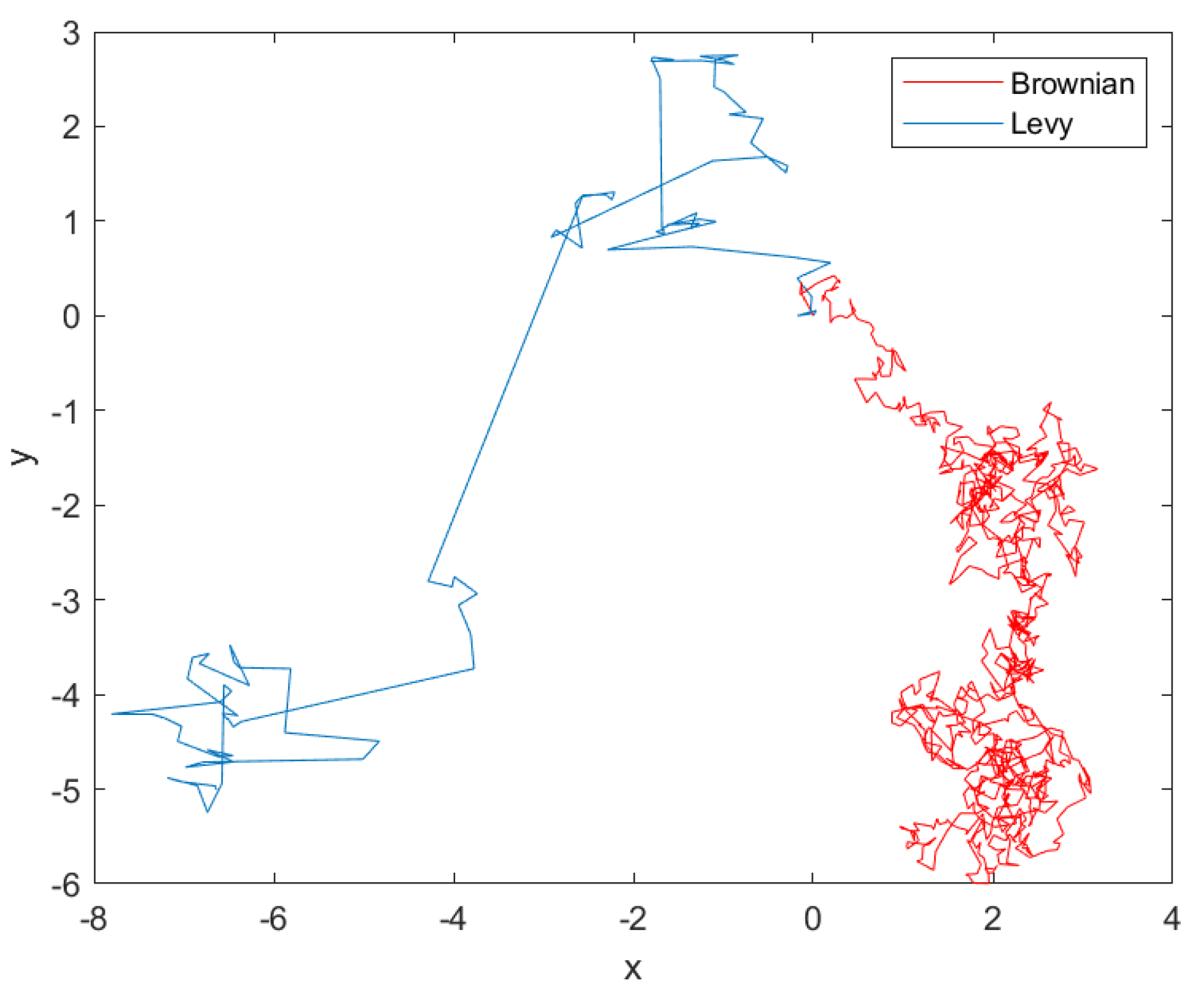
In 2020, Faramarzi et al. introduced a new nature-inspired swarm intelligence metaheuristic using Lévy flight and Brownian motion for model movements of predators in the ocean called the marine predator algorithm (MPA) [13]. The main idea of the MPA is to simulate a typical pattern of foraging of predators (i.e., tuna fish, sunfish, shark, etc.) under the water. Many researchers have found that the most accurate simulation of the moving and food-searching strategy of the marine predators is Lévy flight represented rather by many small steps. Moreover, ‘smooth’ walking in some stages of the particles’ search process enables Brownian motion. Brownian motion enables the sampling of random values by employing the Gaussian distribution function. The Lévy flight provides steps of random walk defined by Lévy distribution with flight length $x_j$ and power-law exponent $\alpha \in (1,2)$:

$$L\left(x_j\right)\approx {\left|x_j\right|}^{1-\alpha }.$$

(2)

Brownian motion and Lévy flight produce a random movement of elements in the predefined search space. The main difference between these two techniques is that whereas Brownian motion is defined by steps of a similar length, Lévy flight enables occasional bigger steps (see Figure 1).

Figure 1. Trajectory of steps for Brownian motion and Lévy flight.

Both methods started from the same position and took steps in different directions. The step size of Brownian motion is more consistent (rather ‘smooth’), whereas Lévy flight produces steps with various sizes.

2.1. Three Phases of MPA

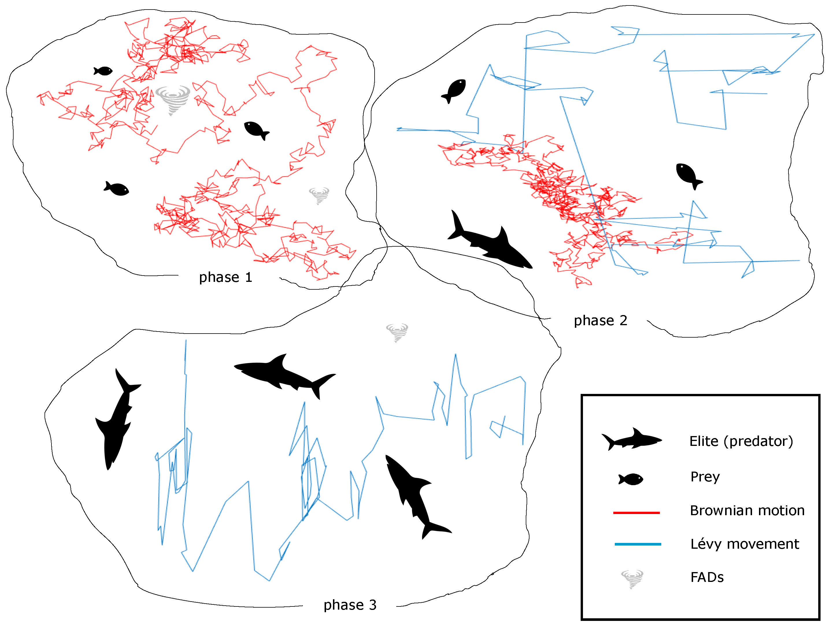
The MPA method belongs to a set of nature-inspired swarm-intelligence population-based optimisation algorithms. As the most population-based algorithms, MPA starts with a randomly initialised population P in the search space $\Omega$. Besides the population (swarm) of predators, the elite predator position ($E\overrightarrow{li}te$) is stored to be used in the moving process. After the initialisation, the update process of the predators’ position started. This process is represented by three phases of moving the predator and prey, as depicted in Figure 2.

Figure 2. Three phases of the marine predator algorithm (MPA).

2.1.1. First Phase

In the first phase, the beginning of the predator’s moving process is initialised. In this phase, the highest velocity (speed) of predator foraging speed is achieved. The idea is to simulate the exploration phase, where the areas of potentially good food sources are detected. This phase of MPA is expected in the first third of the optimisation process when the number of function evaluations (FES) is lower than the total number of function evaluations allocated for the run (maxFES). Then, the new position of the particle is updated using the current position (${\overrightarrow{x}}_i$) and step:

$${\overrightarrow{x}}_i={\overrightarrow{x}}_i+P·rand(0,1)·{\overrightarrow{R}}_B·(E\overrightarrow{li}te-{\overrightarrow{R}}_B·{\overrightarrow{x}}_i)$$

(3)

where $P\in (0,1)$ is the input control parameter of the first stage, ${\overrightarrow{R}}_B$ is the vector of random numbers from Brownian movement, and $E\overrightarrow{li}te$ represents the best particle position in the history of the run.

2.1.2. Second Phase

The second phase occurs when the current number of function evaluations (FES) is in the second third of the run, $\mathit{maxFES}/3\le \mathit{FES}\le 2·\mathit{maxFES}/3$. This phase simulates where prey and predator move similarly because both are foraging the food positions. In this phase, exploration and exploitation occurred, where half the population explored the search space and the second half was used for exploitation. Thus, particles (${\overrightarrow{x}}_i$) in the first half of the population are updated using Lévy flight:

$${\overrightarrow{x}}_i={\overrightarrow{x}}_i+P·rand(0,1)·{\overrightarrow{R}}_L·(E\overrightarrow{li}te-{\overrightarrow{R}}_L·{\overrightarrow{x}}_i)$$

(4)

and the second half of the population is updated, employing the Brownian movement:

$${\overrightarrow{x}}_i=E\overrightarrow{li}te+P·\mathit{CF}·{\overrightarrow{R}}_B·({\overrightarrow{R}}_B·E\overrightarrow{li}te-{\overrightarrow{x}}_i)$$

(5)

where ${\overrightarrow{R}}_L$ and ${\overrightarrow{R}}_B$ are vectors of random numbers from Lévy and Brownian movement, $E\overrightarrow{li}te$ is the position of the best solution, $P\in (0,1)$ is the MPA control parameter, and the control parameter of the predator’s step is $\mathit{CF}={(1-\frac{\mathit{FES}}{\mathit{maxFES}})}^{\left(2\frac{\mathit{FES}}{\mathit{maxFES}}\right)}$.

2.1.3. Third Phase

In the third phase ($\mathit{FES}>2·\mathit{maxFES}/3$), the lowest velocity of particles is achieved. In this scenario, the predator is faster than the prey, i.e., the particles ${\overrightarrow{x}}_i$ follow the update by the exploration phase:

$${\overrightarrow{x}}_i=E\overrightarrow{li}te+P·\mathit{CF}·{\overrightarrow{R}}_L·({\overrightarrow{R}}_L·E\overrightarrow{li}te-{\overrightarrow{x}}_i).$$

(6)

Predators (e.g., sharks) spend much of their lives in Eddy’s formation or fish aggregating devices (FADs). This effect inspired the authors of MPA to add a new enhanced element to the optimiser to avoid stagnation in the area of the local minima.

$${\overrightarrow{x}}_i=\left\{\begin{array}{cc}{\overrightarrow{x}}_i+\mathit{CF}[{\overrightarrow{x}}_{\min }+\overrightarrow{R}·({\overrightarrow{x}}_{\max }-{\overrightarrow{x}}_{\min })]·\overrightarrow{U},\hfill & ifr\le \mathit{FADs}\hfill \\ {\overrightarrow{x}}_i+[\mathit{FADs}(1-r)+r]({\overrightarrow{x}}_{\mathrm{r}1}-{\overrightarrow{x}}_{\mathrm{r}2}),\hfill & \mathit{otherwise}.\hfill \end{array}\right.$$

(7)

where $\mathit{FADs}=0.2$ is the probability of the FADs effect, vector $\overrightarrow{U}$ contains random values from $(0,1)$ transformed to 0 if they are under $0.2$ or 1, ${\overrightarrow{x}}_{\max }$ and ${\overrightarrow{x}}_{\min }$ are vectors with maximal and minimal values of prey locations, and $r1,r2$ are randomly selected indices of prey. For better illustration, the flowchart of the MPA algorithms is depicted in Figure 3.

Figure 3. Flowchart of the marine predator algorithm.

Briefly, the phases of the MPA enable exploration of the search space, moving the prey in the first phase (see Figure 1). Both prey and predators search for their food sources (half of the population works on exploration and half on exploitation). Finally, predators exploit the allocated food areas (switching from Brownian to Lévy steps).

The MPA algorithm was successfully enhanced and applied to many various optimisation problems. Some examples of the most popular MPA experiments are presented as follows.

2.2. Applications of MPA

In 2020, Abdel-Basset et al. proposed a new hybrid model of the improved marine predator algorithm (MPA) to detect COVID-19 [14]. The new variant of MPA introduced a ranking-based mechanism for faster convergence of the population towards the best solution. A new IMPA variant was used to detect COVID-19 in the X-ray images of the human lungs. The proposed IMPA outperformed five nature-inspired optimisers and also the original MPA variant.

In 2020, Al-qaness et al. proposed a model MPA with an Adaptive Neuro-Fuzzy Inference System (ANFIS) to forecast the number of COVID-19 cases in four world countries—Italy, USA, Iran, and Korea [15]. Standard time-series quantifiers measured the quality of the estimated numbers. The proposed MPA-ANFIS model is compared with ABC, ANFIS, FPASSA, GA, PSO, and SCA. The results illustrate that the proposed MPA-ANFIS is not the fastest method, but it provides the most accurate forecast of the COVID-19 case numbers in these countries.

In 2020, Sahlol et al. introduced an enhanced MPA variant to classify the COVID-19 images [16]. The authors combined convolutional neural networks (CNN) with MPA to develop a new FO-MPA optimiser. The proposed method is applied to X-ray COVID-19 images from two Kaggle datasets. The results are compared with nine nature-inspired algorithms, including the original MPA. The proposed FO-MPA provided the best mean results. Only the Harris Hawk optimiser and the original MPA found better solutions.

In 2020, Elaziz et al. proposed a model of MPA cooperating with the moth–flame optimiser (MFO) [17]. A newly designed MPAMFO was applied to the segmentation of CT images of COVID-19 cases. The results are compared with eight nature-inspired methods, including the original MPA and MFO. The proposed MPAMFO provided the most robust results in several levels of thresholding of human head CT images.

In 2020, Yousri et al. simulated applying the MPA optimiser to achieve the maximal energy of photovoltaic plants [18]. The performance of MPA is measured by the simulation of $9\times 9$, $16\times 16$, and $25\times 25$ arrays and compared with three optimisers (MRFO, HHO, and PSO) and the regular TCT connection. The results illustrated that the MPA is the best-performing method that reduces time complexity by 5–20%.

In 2020, Soliman et al. employed the MPA to estimate the parameters of two different marketable triple-diode photovoltaic systems [19]. The experiment’s results are compared with those of four nature-inspired methods. The authors concluded that the MPA can provide accurate results for any marketable photovoltaic system.

In 2020, Abdel-Basst et al. proposed an energy-aware model of MPA to solve the task scheduling of fog computing [20]. The authors introduced two MPA versions—the first improved exploitation capability using the last updated positions instead of the best one. The second used a ranking-based strategy and mutation with the random regeneration of part of the population after a predefined number of iterations. Three MPA variants are compared with five nature-inspired algorithms. The results illustrated the high performance of the proposed MPA variants.

In 2021, Qinsong et al. proposed a modified variant of MPA with an opposition-based learning (OBL) approach based on chaotic maps [21]. Besides OBL, a new updated process of individuals using an inertia weight coefficient was performed. Further, a nonlinear step size for balance between exploration and exploitation was introduced. The efficiency of the new MMPA was measured by artificial problems (CEC 2020) and four engineering problems. The results illustrated the MMPA superiority on most optimisation tasks.

In 2021, Abd Elminaam et al. proposed a new variant of MPA using a k-nearest neighbor strategy [22]. This approach enables the classification of records of the training datasets using Euclidean distances. A new MPA-kNN variant was applied to 18 datasets to classify features and instances. The results were compared with seven other metaheuristics, and the proposed MPA achieved the best performance.

In 2023, Aydemir et al. introduced an elite evolution strategy approach for MPA when solving engineering problems [23]. The idea was to introduce a random mutation for elite individuals, controlling the convergence of MPA. The proposed MPA variant was applied to CEC 2017 problems and several engineering problems. Achieved results were compared with several counterparts and illustrated the performance of the new MPA.

In 2023, Kumar et al. introduced a new variant of MPA with chaotic maps for engineering problems [24]. The idea was to employ a chaos approach in MPA to avoid repeated locations (positions) during the search. The CMPA only has control parameter $P_c$ to control the amount of chaos used in the search process. Twelve various chaos settings were used to achieve the best performance in engineering problems. The results illustrate that different CMPA chaos settings achieved the best results in different engineering problems.

The authors of these studies focused on applying the MPA algorithms to various optimisation problems. The studies did not analyse the setting of the MPA parameters for practical (real-world) use. In this paper, a comprehensive analysis of the MPA control parameters is performed to illustrate the proper setting of this optimiser for future applications. Thirteen real-world engineering optimisation problems were used to illustrate the performance of various MPA settings.

3. MPA Control Parameters

The MPA algorithm is controlled by several control parameters (see Equations (3)–(7)). Besides the population size N, three crucial numerical parameters play a significant role in the performance of this optimiser when searching for the solution to the problems. The aim of this paper is to study various MPA settings to achieve insight into the efficiency of this optimiser when solving engineering problems. Therefore, several rather equidistant values were proposed for each MPA numerical parameter and combined with the remaining parameters. Various (small, middle, and large) values of the MPA numerical parameters were employed.

3.1. Fish Aggregating Devices Strategy

The first parameter studied here is called $\mathit{FADs}\in (0,1)$, employed in Equation (7). This value helps the predators to employ the fish aggregating device (FAD) strategy. The authors recommended the value of $\mathit{FADs}=0.2$. Three fixed values are studied in the presented experiment, $\mathit{FADs}=(0.2,0.5,0.8)$. Moreover, six linear-change settings are used, where the value of the FAD is linearly updated (increased or decreased) during the search process: (0-1), (1-0), (0-0.5), (0.5-1), (1-0.5), (0.5-0).

3.2. Velocity of Particles

The velocity of predator and prey individuals in the MPA is controlled by $P\in (0,1)$, and the authors recommended setting $P=0.5$. This parameter is used in Equations (3)–(6). In this study, two more interesting values of this parameter are added. Therefore, three fixed values are used in the experiment, $P=(0.1,0.5,0.9)$. Further, six linear change settings are investigated, where the value is linearly updated (increased or decreased) during the search process: (0-1), (1-0), (0-0.5), (0.5-1), (1-0.5), (0.5-0).

3.3. Lévy Flight

The Lévy flight strategy is used to move particles in the second and third phases (see Equations (4) and (6). This movement strategy is based on the vector of ${\overrightarrow{R}}_L$, controlled by the parameter $\beta$. The authors of MPA recommended using $\beta =1.5$, three fixed values are used in this study, $\beta =(1,1.25,1.5)$. Moreover, six linear change settings of the $\beta$ parameter are used, where the value is linearly updated (increased or decreased) during the search process: (0-1.5), (1.5-0), (0-0.75), (0.75-1.5), (1.5-0.75), (0.75-0).

4. Experiment Settings

This study aims to analyse the performance of three crucial MPA control parameters. As described above, several various settings of P, FADs, and $\beta$ were mentioned in the experiment. In total, 188 combinations of the MPA control parameters were employed for this study. Moreover, five variants of MPA with the recommended settings and linearly decreased population size are also included in the comparison. Four numbers distinguish variants of MPA to make the experiment results more transparent. Variants of the MPA algorithm are labelled by ‘(MPA_)N_FADs$\_P\_\beta$’. For example, ‘MPA_10_0.2$\_0.5\_1.5$’ (or ‘$10\_0.2\_0.5\_1.5$’) denotes the original settings of MPA with population size $N=10$.

Thirteen real-world engineering problems were selected for this study to show the performance of the MPA variants. All the problems are minimisation, i.e., the minimal function value is searched. For each problem and MPA setting, 30 independent runs are performed to achieve robustness of the statistical comparison. The run is divided into 11 equidistant stages to illustrate the performance of the methods during the search process. For each run of the algorithm and problem, the solution was achieved when $FES=9000$ number of function evaluations was reached. These real-world engineering problems were also collected for another study, where more detail is provided [25]. All the problems are represented by constrained problems, where search space $\Omega$ is bounded by linear and nonlinear limits to define feasible areas. The dimensionality of these problems (D) and function value of true solution ($f\left({\overrightarrow{x}}^{*}\right)$) are provided in Table 1.

Table 1. Detail of real-world engineering problems—dimensionality D and true solution $f\left({\overrightarrow{x}}^{*}\right)$ [25].

Problem	D	$\mathit{f}\left({\overrightarrow{\mathit{x}}}^{*}\right)$
Speed reducer design (Figure 4)	7	2994.4244658
Tension/compression spring design	3	0.012665232788
Pressure vessel design	4	6059.714335048436
Three-bar truss design (Figure 4)	2	263.89584338
Gear train design (Figure 5)	4	2.70085714 × 10−12
Cantilever beam (Figure 5)	5	1.3399576
Minimise I-beam vertical deflection	4	0.0130741
Tubular column design (Figure 6)	2	26.486361473
Piston lever (Figure 6)	4	8.41269832311
Corrugated bulkhead design	4	6.8429580100808
Car side impact design (Figure 7)	11	22.84296954
Welded beam design	4	1.724852308597366
Reinforced concrete beam design (Figure 7)	3	359.2080

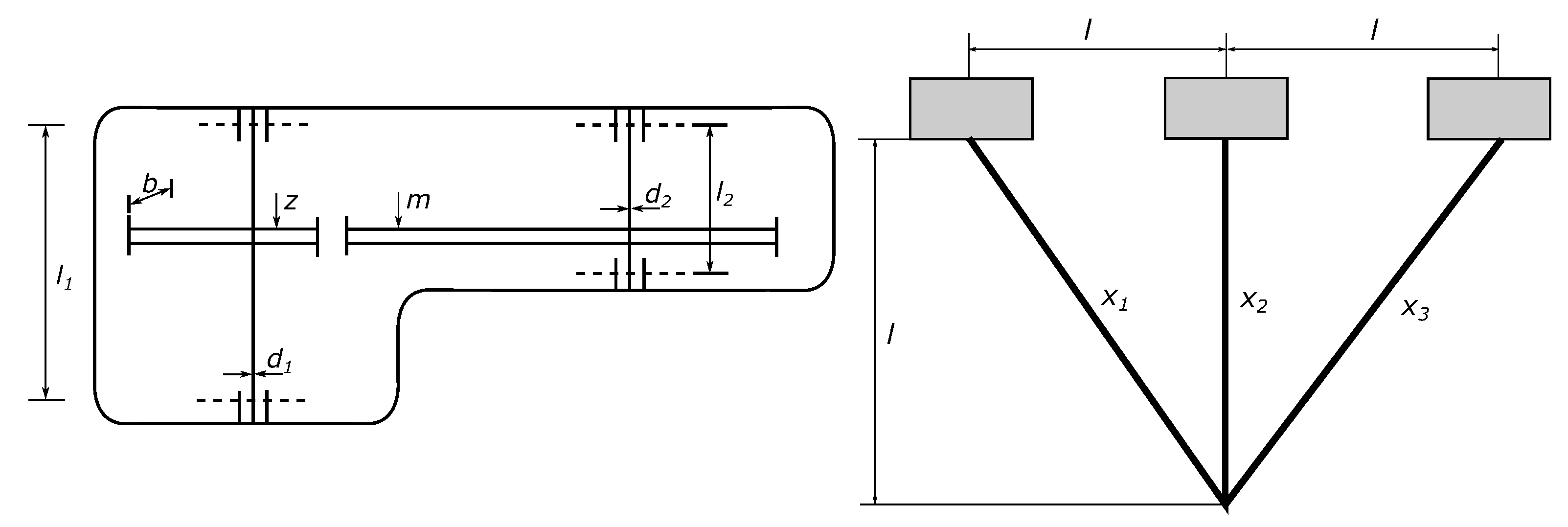
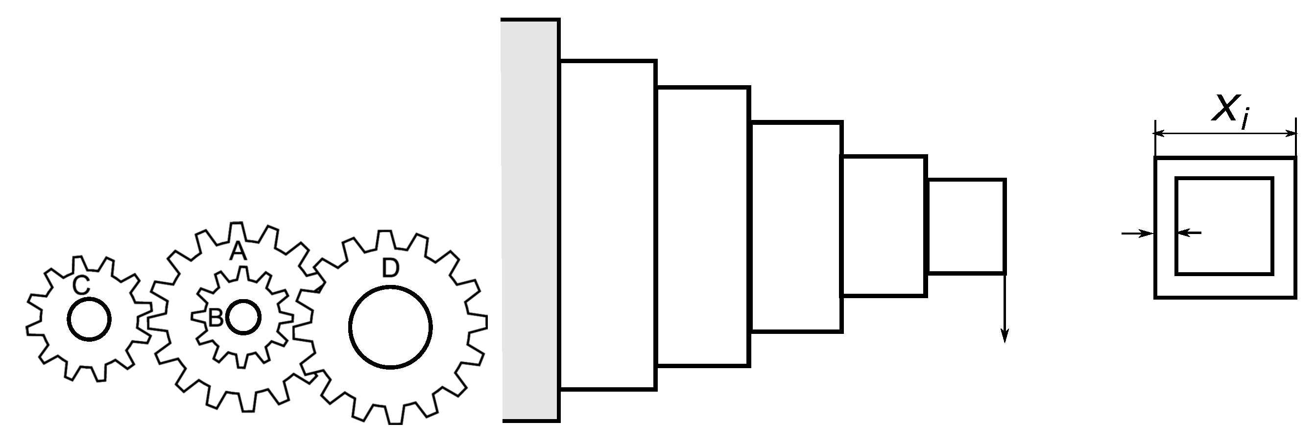
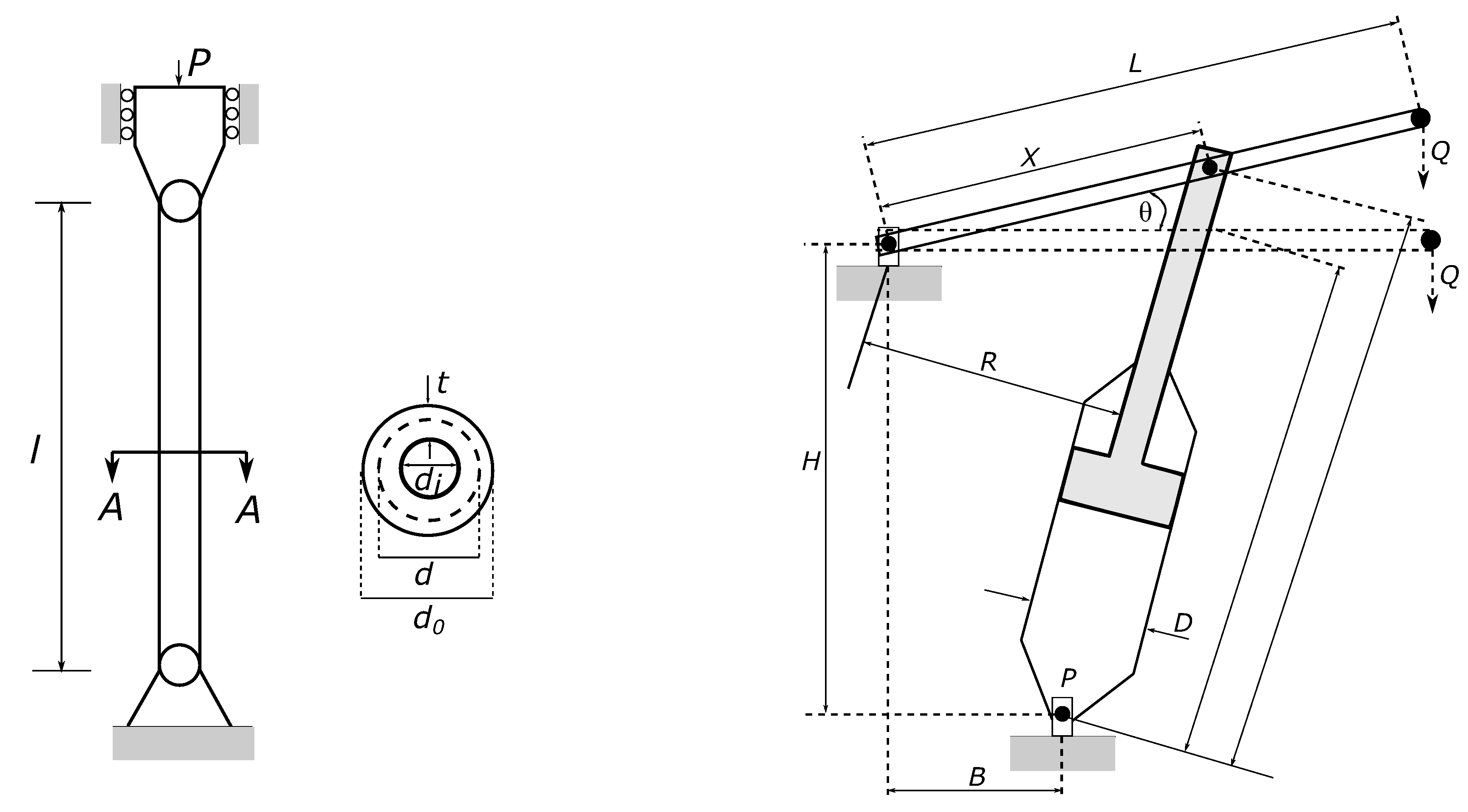
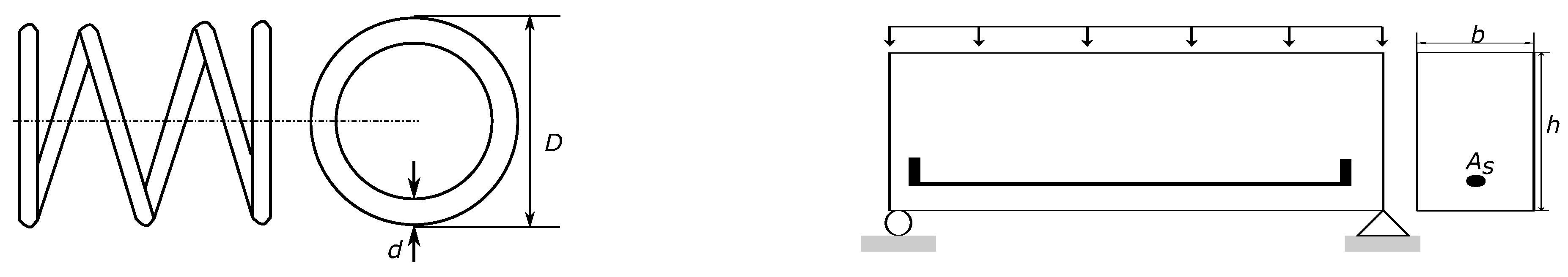
The dimensionality of the selected engineering problems is rather low ($2\le D\le 11$). It causes lower complexity, where the movement of particles in a low-dimensional space is faster. For a better illustration, the design of six engineering problems is provided in Figure 4, Figure 5, Figure 6 and Figure 7.

Figure 4. Speed reducer design problem and three-bar truss problem.

Figure 5. Gear train design problem and cantilever beam design problem.

Figure 6. Tubular columns design problem and piston lever problem.

Figure 7. Tension/compression spring design problem and concrete beam design problem.

5. Results

This study compares 193 MPA variants with various settings of the control parameters when solving 13 real-world engineering optimisation problems. The experiment provides a huge amount of data results to analyse. An advanced statistical comparison is performed instead of standard descriptive values and plots for better illustration. At first, the absolute mean ranks from the Friedman tests of all 193 MPA settings are provided for each stage separately inTable 2, Table 3, Table 4 and Table 5.

Table 2. Absolute mean ranks from the Friedman tests of 11 stages.

N	FADs	P	$\mathit{\beta }$	AR1	AR2	AR3	AR4	AR5	AR6	AR7	AR8	AR9	AR10	AR11
10	0.2	$0.5\_0$	1.5	1	2	2	3	1	1	1	1	1	1	1
10	0.2	$0.5\_1$	1.5	13	14	17	7	9	7	8	2	3	2	2
10	0.2	$1\_0$	1.5	19	22	23	14	10	9	10	14	8	3	3
10	0.2	0.5	1.5	10	5	13	11	11	12	11	9	4	4	4
10	0.2	0.5	$1.5\_0.75$	4	6	4	6	5	5	5	4	2	5	5
10	0.2	0.5	1	6	3	8	1	2	4	4	3	5	6	6
10	0.2	0.5	1.25	3	4	3	2	7	3	3	5	6	7	7
10	0.2	0.1	1.5	20	18	9	10	14	13	16	13	9	8	8
10	0.2	0.5	1.5	14	7	5	5	8	6	6	8	10	9	9
10	0.2	0.5	$0\_1.5$	12	9	8	8	7	2	2	6	8	10	10
10	0.2	0.9	1	18	15	19	18	15	14	12	8	11	11	11
10	0.2	$0.5\_0$	$1.5\_0.75$	9	10	6	13	12	8	9	11	12	12	12
10	0.2	$1\_0.5$	1.5	23	23	24	24	21	20	18	18	14	13	13
10	0.2	0.5	$0\_0.75$	15	13	10	15	4	10	7	11	13	14	14
10	0.2	0.5	$0.75\_0$	5	11	18	13	18	17	17	20	20	15	15
10	0.2	0.5	$0.75\_1.5$	8	12	14	16	16	15	13	13	17	16	16
10	0.2	0.5	$1.5\_0$	11	16	12	9	13	16	15	16	16	17	17
10	0.2	0.9	1.25	22	17	22	17	20	18	19	19	19	18	18
10	0.2	0.9	1.5	21	20	20	19	19	19	21	23	22	19	19
$19\_5$	0.2	0.5	1.5	24	27	27	25	25	23	22	16	15	20	20
10	$0.5\_0$	0.5	1.5	28	26	26	27	26	24	24	22	21	21	21
10	$0\_0.5$	0.5	1.5	2	1	1	4	3	11	14	17	18	22	22
10	0.2	0.1	1	17	19	15	23	23	21	23	24	23	23	23
10	0.2	0.1	1.25	16	21	16	21	18	22	20	21	24	24	24
10	0.2	$0\_1$	1.5	25	25	21	22	22	25	25	25	25	25	25
10	0.5	0.5	1.25	32	29	29	29	29	29	29	29	27	26	26
10	0.5	0.9	1.5	37	36	32	32	34	34	32	32	30	27	27
10	0.5	0.1	1.5	29	28	28	28	28	28	28	27	26	28	28
10	0.5	0.5	1	33	33	30	31	31	31	30	30	28	29	29
10	0.5	0.9	1	36	37	36	34	32	33	34	33	34	30	30
10	0.5	0.9	1.25	35	34	33	33	33	32	33	34	33	31	31
10	0.5	0.5	1.5	31	30	31	30	30	30	31	31	32	32	32
10	$1\_0$	0.5	1.5	47	46	42	38	36	36	35	35	35	33	33
10	0.2	$0\_0.5$	1.5	30	24	25	26	27	27	27	28	32	34	34
10	$0\_1$	0.5	1.5	7	8	11	20	25	26	26	26	29	35	35
10	0.5	0.1	1	26	31	37	36	37	37	37	37	36	36	36
10	0.5	0.1	1.25	27	32	35	37	38	38	38	36	37	37	37
10	$1\_0.5$	0.5	1.5	48	51	57	48	47	44	41	39	39	38	38
$97\_5$	0.2	0.5	1.5	76	72	74	71	65	65	50	48	40	39	39
10	$0.5\_1$	0.5	1.5	34	35	34	35	35	35	36	38	38	40	40
$97\_10$	0.2	0.5	1.5	75	69	73	70	67	69	63	52	49	41	41
50	0.2	$0.5\_0$	1.5	58	50	51	49	49	49	49	47	47	42	42
10	0.8	0.5	1	38	38	38	41	40	40	40	41	41	43	43
10	0.8	0.5	1.5	39	40	41	39	39	39	39	40	42	44	44
10	0.8	0.5	1.25	41	39	39	40	41	41	42	43	43	45	45
10	0.8	0.9	1.5	40	41	41	42	43	43	45	44	44	46	46
50	0.2	$1\_0$	1.5	57	68	58	53	53	57	51	51	52	47	47
10	0.8	0.9	1.25	44	42	43	44	44	46	43	42	45	48	48
10	0.8	0.1	1.5	42	43	44	46	42	47	46	46	46	49	49
10	0.8	0.1	1.25	43	45	46	47	48	48	48	49	48	50	50
10	0.8	0.1	1	46	47	47	45	46	45	47	50	50	51	51
10	0.8	0.9	1	45	44	45	43	45	42	44	45	52	52	52
50	$0.5\_0$	0.5	1.5	78	75	72	74	73	73	70	68	57	53	53
50	0.2	0.5	1.25	49	55	52	51	51	50	53	55	58	54	54
50	0.2	0.5	$1.5\_0.75$	63	57	61	55	50	52	58	62	53	55	55

Table 3. Absolute mean ranks from the Friedman tests of 11 stages.

N	FADs	P	$\mathit{\beta }$	AR1	AR2	AR3	AR4	AR5	AR6	AR7	AR8	AR9	AR10	AR11
50	0.2	0.5	1	55	59	65	64	59	60	55	60	59	56	56
50	0.2	0.5	$0.75\_0$	65	61	54	57	54	51	54	58	54	57	57
50	0.2	$0.5\_0$	$1.5\_0.75$	51	52	56	54	52	55	52	54	55	58	58
50	0.2	0.5	1.5	52	49	50	50	60	56	56	53	56	59	59
50	0.2	0.5	1.5	54	54	60	60	61	63	69	56	60	61	61
50	0.2	0.5	$0\_0.75$	61	62	66	56	57	61	64	64	62	61	61
50	0.2	0.5	$0.75\_1.5$	71	63	64	66	64	54	63	66	61	62	62
50	0.2	0.5	$1.5\_0$	69	60	49	59	56	62	60	65	67	63	63
50	0.2	0.5	$0\_1.5$	67	64	55	59	58	53	59	60	63	64	64
50	0.2	0.1	1.5	86	74	70	65	69	68	61	61	65	65	65
50	0.2	0.9	1.25	56	65	68	73	67	67	71	71	69	66	66
50	0.2	0.1	1	81	71	69	67	62	66	57	57	66	67	67
50	0.2	$1\_0.5$	1.5	62	67	63	72	72	71	68	69	64	68	68
50	0.2	0.1	1.25	81	73	71	64	70	64	65	63	70	69	69
50	0.2	$0.5\_1$	1.5	66	66	53	68	64	58	67	67	68	70	70
50	0.2	0.9	1	50	58	67	62	71	70	72	72	71	71	71
50	0.2	0.9	1.5	53	56	62	61	68	72	73	73	72	72	72
$195\_5$	0.2	0.5	1.5	107	103	122	111	114	90	89	85	81	73	73
50	$0\_0.5$	0.5	1.5	72	48	48	52	55	59	66	70	73	74	74
50	0.2	$0\_0.5$	1.5	128	86	78	76	76	74	74	74	75	75	75
50	0.2	$0\_1$	1.5	96	79	75	75	75	76	75	75	74	76	76
$195\_10$	0.2	0.5	1.5	110	114	118	118	106	89	88	84	81	77	77
50	$1\_0$	0.5	1.5	95	101	107	90	87	86	83	80	76	78	78
50	0.5	0.1	1.5	87	84	81	80	80	82	77	76	77	79	79
50	0.5	0.1	1	94	85	80	82	79	80	79	81	79	80	80
100	0.2	$0.5\_0$	1.5	133	104	105	106	98	87	87	89	86	81	81
50	0.5	0.1	1.25	93	82	83	81	82	79	76	79	82	82	82
50	0.5	0.5	1.5	73	70	76	79	78	77	80	77	78	83	83
50	0.5	0.5	1	59	77	79	77	81	81	81	78	83	84	84
100	0.2	$1\_0$	1.5	115	100	101	102	89	91	92	90	90	85	85
50	0.5	0.5	1.25	68	76	77	78	77	78	82	82	84	86	86
50	0.5	0.9	1.5	70	83	84	84	84	85	85	87	88	87	87
50	0.5	0.9	1.25	74	81	85	85	85	84	86	88	89	88	88
50	0.5	0.9	1	60	80	82	84	83	83	84	86	88	89	89
50	$0\_1$	0.5	1.5	64	53	59	69	74	75	78	83	85	90	90
100	0.2	0.5	$1.5\_0.75$	125	112	109	102	90	93	90	91	93	91	91
100	0.2	0.1	1	156	130	120	113	102	103	98	96	95	92	92
100	0.2	0.5	1	109	113	89	92	97	98	93	94	92	93	93
100	0.2	0.5	1.5	89	95	91	89	94	102	94	93	99	94	94
100	0.2	0.1	1.5	127	126	113	116	101	95	100	100	96	95	95
100	$0.5\_0$	0.5	1.5	136	123	123	115	117	116	114	101	97	96	96
100	0.2	0.5	$0.75\_0$	121	110	104	112	91	100	100	92	104	97	97
100	0.2	$0.5\_0$	$1.5\_0.75$	108	115	98	98	95	106	96	95	91	98	98
100	0.2	0.5	1.5	97	108	102	97	99	115	104	104	105	99	99
100	0.2	$1\_0.5$	1.5	106	106	116	99	116	113	102	109	109	100	100
100	0.2	0.5	$0.75\_1.5$	118	93	108	91	100	114	108	103	102	101	101
100	0.2	0.1	1.25	142	128	119	120	104	92	97	102	98	102	102
100	0.2	0.5	1.25	100	92	90	87	88	94	91	97	94	103	103
100	0.2	0.5	$0\_1$.5	122	118	111	110	111	96	103	99	100	104	104
100	0.2	0.5	$0\_0.75$	137	109	115	119	108	109	109	105	103	105	105
50	$1\_0.5$	0.5	1.5	101	107	121	121	119	122	117	116	106	106	106
100	0.2	0.5	$1.5\_0$	119	116	96	114	114	97	106	98	101	107	107
100	0.2	0.9	1.25	92	111	106	109	115	107	110	107	107	108	108
50	0.8	0.1	1	124	105	111	107	112	110	113	111	108	109	109
100	0.2	0.9	1.5	85	99	97	108	105	108	105	108	110	110	110

Table 4. Absolute mean ranks from the Friedman tests of 11 stages.

N	FADs	P	$\mathit{\beta }$	AR1	AR2	AR3	AR4	AR5	AR6	AR7	AR8	AR9	AR10	AR11
100	0.2	0.9	1	91	94	93	88	103	104	107	113	112	111	111
100	0.2	$0.5\_1$	1.5	113	120	112	117	107	111	115	115	113	112	112
50	0.8	0.1	1.5	123	97	99	94	93	99	111	112	115	113	113
50	0.8	0.1	1.25	120	98	94	95	92	101	101	110	111	114	114
100	$0\_0.5$	0.5	1.5	117	117	95	93	96	105	112	114	117	115	115
100	0.2	$0\_0.5$	1.5	191	142	131	126	122	119	123	118	116	116	116
100	0.2	$0\_1$	1.5	175	136	130	129	124	126	126	122	119	117	117
100	0.5	0.1	1.25	153	139	135	131	128	121	121	124	123	118	118
50	0.8	0.5	1.25	82	89	87	96	110	112	116	117	118	119	119
100	$1\_0$	0.5	1.5	162	141	143	136	135	135	134	133	126	120	120
50	0.8	0.5	1	79	89	92	104	118	118	118	123	120	122	122
50	$0.5\_1$	0.5	1.5	77	78	86	86	86	88	95	106	114	122	122
100	0.5	0.1	1.5	144	132	127	124	125	124	122	120	122	123	123
50	0.8	0.5	1.5	83	90	88	100	109	117	120	121	124	124	124
100	0.5	0.1	1	161	140	132	128	127	123	119	119	121	125	125
100	0.5	0.5	1.25	105	129	125	133	133	131	130	132	128	126	126
100	0.5	0.5	1.5	98	124	126	125	129	130	127	126	125	127	127
100	0.5	0.5	1	104	125	129	127	130	129	131	130	130	128	128
50	0.8	0.9	1	88	91	117	122	123	127	128	128	129	129	129
100	0.5	0.9	1.5	103	119	128	130	131	132	132	131	131	130	130
50	0.8	0.9	1.5	90	87	115	123	126	128	129	129	132	131	131
50	0.8	0.9	1.25	84	96	100	104	120	125	124	125	127	132	132
100	0.5	0.9	1	102	122	134	135	134	133	133	134	134	133	133
100	$0\_1$	0.5	1.5	130	102	103	105	121	120	125	127	133	134	134
100	0.5	0.9	1.25	99	121	124	132	132	134	135	135	135	135	135
100	0.8	0.1	1.25	158	147	141	144	141	144	141	140	139	136	136
100	$1\_0.5$	0.5	1.5	167	143	144	143	145	145	139	137	137	137	137
100	0.8	0.1	1.5	166	153	146	146	146	139	145	144	140	138	138
100	0.8	0.5	1	132	137	140	137	137	140	140	136	136	139	139
100	0.8	0.5	1.5	114	133	137	139	140	138	142	143	138	140	140
100	0.8	0.1	1	165	149	145	145	143	137	138	141	141	142	142
100	0.8	0.5	1.25	126	138	143	140	138	143	136	139	142	142	142
100	$0.5\_1$	0.5	1.5	129	127	133	134	136	136	137	138	144	143	143
100	0.8	0.9	1.5	116	135	137	138	144	141	143	142	143	144	144
100	0.8	0.9	1.25	111	134	138	141	142	146	146	146	145	145	145
100	0.8	0.9	1	112	131	139	142	139	142	144	145	146	146	146
500	0.2	$1\_0$	1.5	160	159	156	156	161	163	157	155	151	147	147
500	0.2	0.9	1	131	144	147	147	147	147	148	150	147	148	148
500	0.2	$1\_0.5$	1.5	154	161	155	148	154	149	156	156	154	149	149
500	0.2	0.9	1.25	138	151	148	150	148	148	147	148	150	150	150
500	0.2	0.5	1.5	159	159	158	160	160	153	151	149	148	151	151
500	0.2	0.9	1.5	143	146	150	151	149	152	149	147	149	152	152
500	0.2	$0.5\_0$	1.5	178	181	174	177	183	182	170	166	163	153	153
500	0.2	$0.5\_0$	$1.5\_0.75$	148	161	151	157	159	155	150	155	152	154	154
500	0.2	0.5	$1.5\_0.75$	188	168	175	162	164	160	161	160	158	155	155
500	0.2	0.5	1.25	155	157	157	159	157	158	153	153	155	156	156
500	0.2	0.5	1	151	163	159	158	153	152	155	158	154	157	157
500	0.2	0.5	$1.5\_0$	187	172	179	161	162	165	154	151	161	158	158
500	0.2	0.5	1.5	134	150	153	149	155	150	158	157	156	159	159
500	0.2	0.5	$0.75\_0$	186	179	167	164	173	175	172	164	165	160	160

Table 5. Absolute mean ranks from the Friedman tests of 11 stages.

N	FADs	P	$\mathit{\beta }$	AR1	AR2	AR3	AR4	AR5	AR6	AR7	AR8	AR9	AR10	AR11
500	$0.5\_0$	0.5	1.5	174	173	172	175	179	170	175	169	159	161	161
500	0.2	0.5	$0.75\_1.5$	178	169	163	163	166	172	165	161	162	162	162
500	0.5	0.9	1.5	141	152	154	153	151	156	152	152	157	163	163
500	0.2	0.5	$0\_0.75$	184	180	178	173	176	180	167	162	166	164	164
500	0.2	0.5	$0\_1$.5	190	176	177	170	174	168	180	171	173	165	165
500	0.5	0.5	1.25	150	165	170	171	165	162	162	170	160	166	166
500	0.5	0.9	1	135	148	152	154	158	154	159	163	164	167	167
500	0.2	0.1	1.5	183	185	182	180	178	186	169	165	167	168	168
500	0.2	$0.5\_1$	1.5	180	174	168	168	172	169	177	173	173	169	169
500	$1\_0$	0.5	1.5	182	177	185	182	187	181	185	185	178	170	170
500	$0\_0.5$	0.5	1.5	185	175	171	169	171	173	164	167	170	171	171
500	0.5	0.5	1.5	145	162	160	155	152	159	160	159	168	172	172
500	0.5	0.5	1	146	156	162	166	156	161	166	168	169	173	173
500	0.2	0.1	1.25	170	187	186	186	184	178	179	177	171	174	174
500	0.2	0.1	1	171	182	183	184	177	168	178	175	176	175	175
500	0.5	0.1	1.25	168	183	181	183	182	176	168	172	175	176	176
500	0.5	0.9	1.25	139	145	149	152	151	157	163	174	174	177	177
500	$0\_1$	0.5	1.5	181	171	165	165	180	174	176	179	179	178	178
500	0.2	$0\_1$	1.5	192	193	192	189	190	193	193	192	183	179	179
500	0.8	0.9	1.25	149	154	161	172	168	164	174	176	177	180	180
500	0.2	$0\_0.5$	1.5	193	192	193	191	193	189	188	188	187	181	181
500	0.5	0.1	1.5	173	189	188	188	181	177	184	181	180	182	182
500	0.8	0.9	1	147	155	166	167	163	179	173	183	182	183	183
500	0.8	0.1	1.25	164	188	191	193	191	192	187	187	186	184	184
500	0.5	0.1	1	189	184	184	187	185	184	181	182	188	185	185
500	$0.5\_1$	0.5	1.5	173	179	173	178	188	188	189	190	193	186	186
500	$1\_0.5$	0.5	1.5	176	186	187	185	189	191	191	189	191	187	187
500	0.8	0.1	1.5	179	191	190	192	192	190	190	186	185	188	188
500	0.8	0.1	1	169	190	189	190	186	187	192	193	190	189	189
500	0.8	0.5	1.5	157	166	180	181	175	183	171	180	184	190	190
500	0.8	0.9	1.5	140	164	164	176	169	185	183	178	181	191	191
500	0.8	0.5	1	163	167	169	174	167	166	183	184	189	192	192
500	0.8	0.5	1.25	152	170	177	179	170	171	186	191	192	193	193

Each table row represents one MPA setting, defined by four control parameters in the first four columns. The remaining columns of the table present the absolute mean ranks, where a lower rank means better results of the MPA settings regarding all 13 engineering problems. The rows are sorted using the ranks in the final stage of the run (last column). As such, the best-performing settings are at the top of the table, and the efficiency of the MPA decreases towards the end of the table. The best results provide three MPA settings with the recommended settings of FADs and $\beta$, and linear change of P, (0.5-0), (0.5-1), (1-0). The recommended MPA setting takes the fourth position.

It is possible to provide several remarks regarding MPA parameters:

• The efficiency of MPA is decreased with increasing population size.
• The best linear population size reduction is in the 20th position.
• Twenty of the best MPA variants use recommended $\mathit{FADs}=0.2$.
• Six of the worst performing MPA settings employ $\mathit{FADs}=0.8$.
• Seven out of seventeen of the best-performing MPA variants use a linear change of $\beta$.
• The variant of MPA$10\_0-0.5\_0.5\_1.5$ (original settings and linear change of FADs) achieves good results in the first five search stages. That information is interesting for the cases where the low time demands are provided.

Decreasing the population size of MPA did not provide better results compared to a fixed small population size ($N=10$). Therefore, these variants were removed from the illustration of the mean ranks from the Friedman tests (Figure 8). The settings of all MPA variants are labelled on the axes, where values of $\beta$ and N are on the vertical axis, and P and FADs are on the horizontal axis. The rectangle is divided into nine smaller rectangles based on $\beta$ and P values. Absolute mean ranks denoting the ten best-performing and ten worst-performing MPA variants are included in this figure.

Figure 8. Absolute ranks from the Friedman test computed for 108 combinations of marine predator algorithm control parameter settings.

The mean ranks are evaluated by colour, from the least mean rank (best-performing setting, dark blue) to the biggest mean rank (worst-performing, dark red) setting, according to the colour bar on the right side. Dark blue horizontal rows illustrate the good performance of the small population size. A decreasing saturation of blue from the left to the right side of smaller rectangles means that the efficiency of MPA is decreasing with the increasing value of FAD. Conversely, the smaller rectangles’ colour patterns are similar, which points out the smaller influence of P and $\beta$ parameters. Analysing Table 2, Table 3, Table 4 and Table 5 and Figure 8 results in the selection of the best-performing MPA variants for further analysis.

The absolute ranks of the top nine MPA variants during 11 stages are depicted in Figure 9. The positions of the lines on the right side illustrate the final efficiency of the optimisers, where dots present the recommended original setting. The best setting (10_0.2_0.5-0_1.5) is very efficient during the search process. Surprisingly, the combination of 10_0-0.5_0.5_1.5 (increasing FADs) is very efficient in the early stages, and then it is substantially worse. Oppositely, an efficiency of 10_0.2_1-0_1.5 (decreasing P) is increasing from the worst position to the third place.

Figure 9. Absolute ranks of the best nine marine predator algorithm settings from the Friedman test.

The next step of the MPA variant analysis is to compare the median values of the best-performing settings for each problem separately (Table 6). The median values were computed from the independent runs of the algorithms in the last stage. The results of the original MPA settings are in the first column. Although the variability of the achieved results is not substantial, the best-achieved result for each problem is highlighted.

Table 6. Median values for all problems by nine best-performing marine predator algorithms (MPAs) with given fish aggregating devices, P and $\beta$ (all $N=10$).

Prob.	0.2_0.5_1.5 *	0.2_0.5-0_1.5	0.2_0.5_1	0.2_0.5_1.25	0.2_1-0_1.5	0.2_0.5-1_1.5	0.2_0.5_0-1.5	0.2_0.5_1.5-0.75	0-0.5_0.5_1.5
1	2995.2	2995.335	2994.895	2995.51	2995.09	2995.125	2995.25	2995.115	2995.525
2	0.012668	0.012666	0.0126676	0.012666	0.012667	0.012667	0.012667	0.012666	0.012673
3	6059.72	6059.71	6059.715	6059.71	6059.71	6059.71	6059.71	6059.715	6065.095
4	263.896	263.896	263.896	263.896	263.896	263.896	263.896	263.896	263.896
5	2.7 $\times {10}^{-12}$	2.7 $\times {10}^{-12}$	2.701 $\times {10}^{-12}$	2.7 $\times {10}^{-12}$	2.7 $\times {10}^{-12}$	2.7$\times {10}^{-12}$	2.7 $\times {10}^{-12}$	2.7 $\times {10}^{-12}$	2.7 $\times {10}^{-12}$
6	1.33996	1.33996	1.33998	1.34001	1.339965	1.33997	1.33999	1.339985	1.33997
7	0.013074	0.013074	0.0130743	0.013074	0.013074	0.013074	0.013075	0.013074	0.013075
8	26.4864	26.4864	26.4864	26.4864	26.4864	26.4864	26.4864	26.4864	26.4864
9	8.413115	8.41292	8.41297	8.413095	8.413095	8.413485	8.41324	8.413225	8.4132
10	6.84297	6.84297	6.842975	6.84297	6.84298	6.84297	6.84297	6.842975	6.84299
11	23.0689	22.8922	23.1711	23.19115	23.0341	23.17205	23.08005	23.0662	23.0587
12	1.724885	1.72487	1.72488	1.72488	1.724895	1.72487	1.724895	1.724885	1.724915
13	359.208	359.208	359.208	359.208	359.208	359.208	359.208	359.208	359.208

* The original MPA setting. The best performing MPA variant for each problem is bolded.

The most frequently best-performing MPA variant was 10_0.2_0.5-0_1.5 (five times out of 13). The original setting never achieved the best results separately. Also, the Kruskal–Wallis tests were performed to show significant differences between the nine algorithms for each problem separately. The tests were performed in each stage of the run. The results are significant if the achieved significance level is lower than $0.05$. The significant results in the final stage were only for the 11th problem. Also, there were significant differences in some stages of the problems ($3,6,8,10$).

Finally, the number of first, second, third, and last positions of the nine best-performing MPA variants for each problem and all stages are illustrated in Table 7. The results of the best-performing methods for each problem and stage are highlighted. The algorithms are ordered such that the most frequently best-performing one is on the left side of the table. In most cases, the MPA setting achieved the best results by 10_0.2_0.5-0_1.5, outperforming other MPA variants from the 6th to 11th stage. This setting provides the best results in 28 cases out of 143 (11 stages, 13 problems). On the other side, it achieves the worst results in five cases. Two other combinations of the MPA parameters achieved very promising results in the early stages of the optimisation process: 10_0.2_0.5_1.5-0.75 and 10_0-0.5_0.5_1.5.

Table 7. Number of the best, second best, third, and last positions of the Kruskal–Wallis tests for nine best-performing marine predator algorithms (MPAs) with given fish aggregating devices (FADs), P, and $\beta$ (all $N=10$).

Stage	0.2_0.5-0_1.5	0.2_0.5_1.5-0.75	0-0.5_0.5_1.5	0.2_1-0_1.5	0.2_0.5_1	0.2_0.5_1.25	0.2_0.5_1.5 *	0.2_0.5-1_1.5	0.2_0.5_0-1.5
1	2/1/4/0	1/4/0/0	4/2/1/0	1/0/3/6	1/1/2/1	2/1/2/2	2/1/0/1	0/0/0/0	0/3/1/3
2	3/1/0/0	1/2/1/1	3/2/1/1	1/0/0/6	1/1/2/0	1/0/5/0	0/2/1/2	1/2/1/2	0/1/0/1
3	1/2/0/1	3/0/1/1	4/1/3/0	1/0/0/3	0/1/2/1	1/2/1/1	0/1/0/2	0/2/1/1	0/1/2/1
4	2/0/3/0	3/1/0/0	2/2/2/1	2/0/0/3	1/2/2/0	0/5/0/1	0/0/1/2	0/0/1/1	0/0/1/3
5	1/3/1/0	3/1/0/1	2/1/2/1	1/1/1/3	2/1/1/0	0/2/2/1	0/0/0/1	0/0/2/0	0/0/0/3
6	2/3/1/1	2/1/1/2	1/1/2/3	2/0/0/3	1/2/0/0	1/1/1/0	0/0/1/0	0/0/2/0	0/1/1/1
7	3/1/1/1	2/1/1/1	0/1/1/3	2/0/1/2	1/2/0/1	1/2/1/0	0/0/0/1	0/1/1/0	0/1/3/1
8	3/1/1/1	2/1/2/1	0/0/1/3	1/1/0/2	2/1/0/1	1/3/0/1	0/1/1/0	0/1/2/0	0/0/2/1
9	3/2/0/1	2/1/0/0	0/0/1/5	1/1/0/1	2/1/0/0	1/2/2/2	0/1/3/0	0/1/1/0	0/0/2/1
10	4/0/1/0	1/0/2/0	0/0/0/6	1/2/2/0	1/1/0/0	2/2/0/3	0/2/0/0	0/2/1/0	0/0/3/1
11	4/0/1/0	1/0/2/0	0/0/0/6	1/2/2/0	1/1/0/0	2/2/0/3	0/2/0/0	0/2/1/0	0/0/3/1
$\Sigma$	28/14/13/5	21/12/10/7	16/10/14/29	14/7/9/29	13/14/9/4	12/22/14/14	2/10/7/9	1/11/13/4	0/7/18/17

* The original MPA setting. The best performing MPA variant for each stage is bolded.

More details on the MPA performance of the nine best-performing variants come from the two-sample non-parametric Wilcoxon test. The recommended (original) MPA setting is compared with the remaining variants separately on each problem (Table 8). A number of better results (bet.), significantly better results from the Wilcoxon tests (s.bet.), worse results (wor.), and significantly worse (s.wor.) results of eight newly proposed MPA variants are provided. The methods are ordered from better performing on the left side to worse performing on the right side. The MPA variant 10_0.2_0.5-0_1.5 achieved similar results to the second MPA 10_0.2_1-0_1.5, which was three times outperformed by the original MPA. The variant MPA 10_0.2_0.5_1.5-0.75 achieved the same number of wins (4) and loses (4) compared to the original MPA.

Table 8. Number of better, significantly better, worse, and significantly worse cases of nine best performing marine predator algorithms (MPAs) compared with the original setting from the Wilcoxon tests (all $N=10$).

	0.2_0.5-0_1.5	0.2_1-0_1.5	0.2_05-1_1.5	0.2_0.5_1	0.2_0.5_1.25	0.2_0.5_1.5-0.75	0.2_0.5_0-1.5	0-0.5_0.5_1.5
bet.	5	5	5	5	5	4	2	1
s.bet.	1	1	0	0	0	0	0	0
wor.	1	3	3	4	3	4	6	8
s.wor.	0	0	0	0	1	0	0	0

6. Conclusions

This paper studied the performance of the successful swarm-intelligence optimisation heuristic inspired by marine predators (MPA). The study aims to analyse the MPA parameters when solving real-world engineering problems. Besides the population size N, the MPA optimiser uses three numerical parameters—P, FADs, and $\beta$. The authors of MPA recommended $P=0.5$, $\mathit{FADs}=0.2$, and $\beta =1.5$. Although the MPA was introduced when applied to real-world problems, a more comprehensive experimental comparison of various settings was performed.

Four fixed values and the linear reduction of N were used. Further, three fixed values for each of the three MPA parameters were employed, along with six various linear (increase, decrease) settings. Therefore, 193 various settings of the MPA parameters were compared when solving 13 real-world constrained engineering problems. Achieved results were statistically analysed to illustrate significant differences.

The original MPA setting was outperformed by three variants with the linear change of the particle velocity parameter, $P\in \{$(0.5-0), (0.5-1), (1-0)}. Decreasing values of P (from 1 or $0.5$ to 0) illustrate the situation where the MPA individual’s velocity is decreased during the search process. It is interesting that increasing velocity enables us to outperform the original MPA settings. This finding is very interesting to the real applications of this optimiser.

Further, it was found that the MPA performance decreases when a bigger population size is applied. This fact is caused mostly by the small dimensionality of the real-world problems despite the solutions of the engineering problems limited by the feasible regions.

Finally, the efficiency of MPA is low when the higher value of FAD is employed. This parameter directly influences the frequency of using Eddy’s formation and fish aggregating devices during the search process. From Equation (7), it is clear that using FADs causes a random position of the current solution, which is slowing down the convergence of the MPA population.

A different setting of the $\beta$ parameter has no substantial influence on MPA results. This parameter is called the power law index, and it controls the Lévy flight process, which is used to generate new positions in the second and third phases. Notice that the value of $\beta$ is from $\beta \in (1,2)$.

The most efficient MPA variant in the comparison (10_0.2_0.5-0_1.5) has robust performance during all 11 stages of the search process (based on the absolute rank). This MPA variant achieved the best solution in 5 problems out of 13. Better results were achieved by variant 10_0.2_0.5_1 on the first problem.

Achieved results enable us to illustrate the influence of the MPA parameters when solving engineering problems. The linear change of the P value has the potential to be analysed in future research.