On Bilevel Monotone Inclusion and Variational Inequality Problems

Abstract

In this article, the problem of solving a strongly monotone variational inequality problem over the solution set of a monotone inclusion problem in the setting of real Hilbert spaces is considered. To solve this problem, two methods, which are improvements and modifications of the Tseng splitting method, and projection and contraction methods, are presented. These methods are equipped with inertial terms to improve their speed of convergence. The strong convergence results of the suggested methods are proved under some standard assumptions on the control parameters. Also, strong convergence results are achieved without prior knowledge of the operator norm. Finally, the main results of this research are applied to solve bilevel variational inequality problems, convex minimization problems, and image recovery problems. Some numerical experiments to show the efficiency of our methods are conducted.

1. Introduction

Let $\mathcal{K}$ be a nonempty, closed, and convex subset of a real Hilbert space $\mathcal{H}$ with inner product $⟨·,·⟩$ and induced norm $\parallel ·\parallel$. Let $\mathcal{F}:\mathcal{K}\to \mathcal{H}$ be an operator. The classical variational inequality problem (VIP) is derived as follows: Find $p^{★}\in \mathcal{K}$, such that

$$\begin{array}{c}\hfill ⟨\mathcal{F}{p}^{★},q-p^{★}⟩\ge 0,\forall q\in \mathcal{K}.\end{array}$$

(1)

We denote by $V(\mathcal{K},\mathcal{F})$ the solution set of the VIP (1). Problem (1) has a wide range of applications; several methods for solving this problem have been developed by many researchers (see [1,2,3] and the references in them).

On the other hand, the monotone inclusion problem (MIP) is formulated as follows: Find $p^{★}\in \mathcal{H}$, such that

$$\begin{array}{c}\hfill 0\in (D+E)p^{★},\end{array}$$

(2)

where $\mathcal{H}$ is a real Hilbert space, $E:\mathcal{H}\to \mathcal{H}$ is a single-valued monotone operator, and $D:\mathcal{H}\to 2^{\mathcal{H}}$ is a maximal monotone operator. We denote by ${(D+E)}^{-1}\left(0\right)$ the solution set of the MIP (2); it is referred to as the set of zero points of $D+E$. Several optimization problems can be reformulated into the MIP (2). Some of these problems include convex minimization problems, equilibrium problems, image/signal processing problems, DC programming problems, split feasibility problems, and variational inequality problems; see [4,5,6]. The numerous applications of this problem have attracted the attention of a large number of researchers in the last few years, and many methods for solving the problem have also been developed; see [7,8,9]. One of the first methods for solving this problem is the forward–backward algorithm (FBA), which is defined by sequence $\left\{p_k\right\}$ as follows:

$$\begin{array}{c}\hfill p_{k+1}={(I+{\lambda }_{k}E)}^{-1}(I-{\lambda }_{k}D)p_k,\end{array}$$

(3)

where ${\lambda }_k>0$ is the step size, and $(I-{\lambda }_{k}D)$ and ${(I+{\lambda }_{k}E)}^{-1}$ are denoted as forward and backward operators (also referred to as resolvent operators), respectively. The FBA for solving the MIP was independently studied by Lion and Mercier [6], and Passty [10]. In recent years, the convergence analysis and modifications of this method have been deeply exploited by many authors; see [4,11,12] and the references in them. We should note that the weak convergence result of method (3) requires the operator (D) to be strongly monotone; that is a strong assumption. In order to weaken this restriction, several methods have been developed by a large number of researchers; see [6,11,13] and the reference therein. One of the first methods considered to weaken this assumption was introduced by Tseng [13]. This method is called the Tseng splitting algorithm; it is also known as the forward–backward–forward method. Precisely, this method is defined as follows:

$$\begin{array}{c}\hfill \left\{\begin{array}{c}{p}_1\in \mathcal{H},\hfill \\ q_k={(I+{\lambda }_{k}E)}^{-1}(I-{\lambda }_{k}D)p_k,\hfill \\ p_{k+1}=q_k+{\lambda }_k(D{p}_k-D{q}_k),\hfill \end{array}\right.\end{array}$$

(4)

where $\left\{{\lambda }_k\right\}$ is the step size, which can be updated automatically by the Armijo-type line-search technique. The author proves the weak convergence result of method (4) when operator D is Lipschitz continuous and monotone, and operator E is a maximal monotone operator. In [14], Zhang and Wang merge the FBA (3) and the projection and contraction method to obtain an iterative method that also surmounts the limitations of the FBA. Precisely, this method is defined as follows:

$$\begin{array}{c}\hfill \left\{\begin{array}{c}{p}_1\in \mathcal{H},\hfill \\ q_k={(I+{\lambda }_{k}E)}^{-1}(I-{\lambda }_{k}D)p_k,\hfill \\ p_{k+1}=p_k-\gamma {\delta }_k{m}_k,\hfill \end{array}\right.\end{array}$$

(5)

where $m_k=p_k-q_k-{\lambda }_k(D{p}_k-D{q}_k)$, ${\delta }_k=\frac{⟨p_k-q_k,m_k⟩}{\parallel m_k{\parallel }^2}$, $\gamma \in (0,2)$; $\left\{{\lambda }_k\right\}$ is a control sequence, operator D is monotone–Lipschitz continuous, and E denotes the maximal monotone operator.

It is important to note that algorithms (4) and (5) only converge weakly in infinite dimensional spaces. However, in machine learning and CT reconstruction, strong convergence is more desirable in infinite dimensional spaces [12]. Therefore, it is necessary to modify (3), such that it can achieve strong convergence in real Hilbert spaces. In the last two decades, so many modifications of the forward–backward method have been constructed to obtain strong convergence results in real Hilbert spaces; see [11,12,15,16] and the references in them.

In recent years, the construction of inertial-based algorithms has attracted massive interest from researchers. The idea of including inertial terms in iterative methods for solving optimization problems was initiated by Polyak [17] and it has been confirmed by numerous authors that the inclusion of an inertial term in a method acts as a boost to the convergence speed of the method. A common feature of the inertial-type algorithm is that the next iteration depends on the combination of two previous iterates; for more details, see [3,18,19]. Many inertial-type algorithms have been studied and numerical tests have demonstrated that the inertial effects on these methods greatly improve their performances; see [1,3,20]. Recently, Lorenz and Pock [17] introduced and studied the following inertial FBA to solve the MIP (2):

$$\begin{array}{c}\hfill \left\{\begin{array}{c}{w}_k=p_k+{\theta }_k(p_k-p_{k-1}),\hfill \\ q_k={(I+{\lambda }_{k}E)}^{-1}(I-{\lambda }_{k}D)p_k.\hfill \end{array}\right.\end{array}$$

(6)

Note that method (6) only convergences weakly in real Hilbert spaces; numerical tests by the authors proved that their method outperforms several existing methods without inertial terms.

Several mathematical problems, such as variational inequality problems, equilibrium problems, split feasibility problems, and split minimization problems, are all special MIP cases. These problems have been applied to solve diverse real-world problems, such as modeling inverse problems arising from phase retrieval, modeling intensity-modulated radiation therapy planning, sensor networks in computerized and data compression, optimal control problems, and image/signal processing problems [21,22,23].

The bilevel programming problem is a constrained optimization problem in which the constrained set is a solution set of another optimization problem. This problem is enriched with many applications in modeling Stackelberg games, the convex feasibility problem, determination in Wardrop equilibria for network flow, domain decomposition methods for PDEs, optimal control problems, and image/signal processing problems [23]. When the first-level problem is a VIP and the second-level problem is a fixed point set of a mapping, then the bilevel problem is known as the hierarchical variational inequality problem. In [24,25,26], Yamada introduced the following method, called the hybrid steepest-descent iterative method, to solve the hierarchical VIP:

$$\begin{array}{c}\hfill p_{k+1}=(I-{\alpha }_k\varrho \mathcal{F})\mathcal{S}{p}_k,\end{array}$$

(7)

where $\mathcal{F}$ is a strongly monotone–Lipschitz continuous operator and $\mathcal{S}$ is a nonexpansive mapping.

In this paper, we consider the problem of solving a VIP over the solution set of the MIP in a real Hilbert space. This problem is formulated as follows:

$$\begin{array}{c}\hfill \mathrm{Find}{p}^{★}\in {(D+E)}^{-1}\left(0\right)\mathrm{such}\mathrm{that}⟨\mathcal{F}{p}^{★},q-p^{★}⟩\ge 0,\forall q\in {(D+E)}^{-1}\left(0\right),\end{array}$$

(8)

where $\mathcal{F}$ is a strongly monotone–Lipschitz continuous operator, D is a monotone–Lipschitz continuous operator, and E is a maximal monotone operator.

Inspired by the inertial technique, the Tseng splitting algorithm, projection, and contraction method, and hybrid steepest decent method, we introduce two efficient iterative algorithms to solve problem (8). We prove the strong convergence results of the suggested method under some standard assumptions on the control parameters. Also, the strong convergence results are achieved without prior knowledge of the operator norm. Instead, the stepsizes are self-adaptively updated. Furthermore, we apply our main results to solve the bilevel variational inequality problem, convex minimization problem, and image recovery problem. We conduct numerical experiments to show the practicability, applicability, and efficiency of our methods. Our results improve, generalize, and unify the results presented in [4,12,13,27], as well as several others in the literature.

This article is organized as follows: In Section 2, we present some established definitions and lemmas that will be useful in deriving our main results. In Section 3, we present the proposed method and establish its convergence analysis. In Section 4, we show the applications of our main results to real-world problems. In Section 5, several numerical tests are carried out in finite and infinite dimensional spaces to demonstrate the computational efficiency of the proposed methods. Lastly, in Section 6, a summary of the obtained results is given.

2. Preliminaries

Let $\mathcal{K}$ be a nonempty, closed, and convex subset of a real Hilbert space $\mathcal{H}$. We represent the weak and strong convergence of $\left\{p_k\right\}$ to p by $p_k\rightharpoonup p$ and $p_k\to p$, respectively. For every point $p\in \mathcal{H}$, the unique nearest point, which is denoted by ${\mathcal{P}}_{\mathcal{K}}p$, exists in $\mathcal{K}$, such that $\parallel p-{\mathcal{P}}_{\mathcal{K}}p\parallel \le \parallel p-q\parallel ,\forall q\in \mathcal{K}$. The mapping ${\mathcal{P}}_{\mathcal{K}}$ is called the metric projection of $\mathcal{H}$ onto $\mathcal{K}$ and it is known to be nonexpansive.

Lemma 1

([28]). Let $\mathcal{H}$ be a real Hilbert space and $\mathcal{K}$ a nonempty closed convex subset of $\mathcal{H}$. Suppose $p\in \mathcal{H}$ and $q\in \mathcal{K}$. Then $q=P_{\mathcal{K}}p$⇔$⟨p-q,q-w⟩\ge 0$, $\forall w\in \mathcal{K}$.

Lemma 2

([28]). Let $\mathcal{H}$ be a real Hilbert space. Then for every $p,q\in \mathcal{H}$ and $\sigma \in \mathbb{R}$, we have

(i) 

${\parallel p+q\parallel }^2\le {\parallel p\parallel }^2+2⟨q,p+q⟩$;

(ii) 

${\parallel p+q\parallel }^2={\parallel p\parallel }^2+2⟨p,q⟩+{\parallel q\parallel }^2$;

(iii) 

${\parallel \sigma u+(1-\sigma )v\parallel }^2={\sigma \parallel p\parallel }^2+{(1-\sigma )\parallel q\parallel }^2-\sigma (1-\sigma ){\parallel p-q\parallel }^2$.

Lemma 3

([29]). Let $\left\{a_k\right\}$ be a sequence of non-negative real numbers, such that

$$a_{k+1}\le (1-{\nu }_k)a_k+{\nu }_k{b}_k,\forall k\ge 1,$$

where $\left\{{\nu }_k\right\}\subset (0,1)$ with ${\sum }_{k=0}^{\infty }{\nu }_k=\infty$. If $\underset{k\to \infty }{lim\; sup}{b}_k\le 0$ for every subsequence $\left\{a_{k_j}\right\}$ of $\left\{a_k\right\}$, the following inequality holds:

$$\underset{j\to \infty }{lim\; inf}(a_{k_{j+1}}-a_{k_j})\ge 0,$$

then $\underset{k\to \infty }{lim}{a}_k=0$.

Definition 1.

Let $\mathcal{H}$ be a real Hilbert space and $\mathcal{F}:\mathcal{H}\to \mathcal{H}$ be a mapping. Then, $\mathcal{F}$ is called

(1) 

L-Lipschitz continuous, if $L>0$ exists, such that

$$\parallel \mathcal{F}p-\mathcal{F}q\parallel \le L\parallel p-q\parallel ,\forall p,q\in \mathcal{H}.$$

If $L\in [0,1)$, then $\mathcal{F}$ is a contraction.

(2) 

η-strongly monotone, if there exists a constant $\eta >0$, such that

$$⟨p-q,\mathcal{F}p-\mathcal{F}q⟩\ge {\eta \parallel p-q\parallel }^2,\forall p,q\in \mathcal{H}.$$

(3) 

η-inverse strongly monotone (η-co-coercive), if there exists a constant $\eta >0$, such that

$$⟨p-q,\mathcal{F}p-\mathcal{F}q⟩\ge {\eta \parallel \mathcal{F}p-\mathcal{F}q\parallel }^2,\forall p,q\in \mathcal{H}.$$

(4) 

Monotone, if

$$⟨\mathcal{F}p-\mathcal{F}q,p-q⟩\ge 0,\forall p,q\in \mathcal{H}.$$

Definition 2.

Let $E:\mathcal{H}\to 2^{\mathcal{H}}$ be a multi-valued operator. Then

(a) 

The graph of E is defined by

$$\mathit{Graph}\left(E\right)=\left\{\right(p,q)\in \mathcal{H}\times \mathcal{H}:p\in \mathcal{H},q\in E(p\left)\right\}.$$

(b) 

Operator E is said to be monotone if

$$⟨p-q,y-z⟩\ge 0,\forall y,z\in \mathcal{H},p\in E\left(y\right),q\in E\left(z\right).$$

(c) 

Operator E is said to be maximal monotone if E is monotone and its graph is not a proper subset of the graph of any of the monotone operators.

(d) 

For all $p\in \mathcal{H}$, the resolvent of E is a single-valued mapping $J_{\lambda }^E:\mathcal{H}\to \mathcal{H}$ defined by

$$J_{\lambda }^E\left(p\right)={(I+\lambda E)}^{-1}\left(p\right),$$

where $\lambda >0$ and I is an identity operator on $\mathcal{H}$.

Lemma 4

([30]). Let $E:\mathcal{H}\to 2^{\mathcal{H}}$ be a maximal monotone mapping and $D:\mathcal{H}\to \mathcal{H}$ be a monotone and L-Lipschitz continuous operator. Then, the mapping $D+E$ is a maximal monotone mapping.

Lemma 5

([31]). Suppose that $\varrho >0,\alpha \in (0,1)$, and $\mathcal{F}:\mathcal{H}\to \mathcal{H}$ is η-strongly monotone and $L_1$ continuous, such that $0<\eta \le L_1$. Then for any nonexpansive mapping $S:\mathcal{H}\to \mathcal{H}$, we can associate a mapping $S^{\varrho }:\mathcal{H}\to \mathcal{H}$ defined by $S^{\varrho }p=(I-\alpha \varrho \mathcal{F})\mathcal{S}{p}_k,\forall p\in \mathcal{H}$. Then, $S^{\varrho }$ is a contraction provided $\varrho <\frac{2\eta }{L_1^2}$; that is,

$$\begin{array}{c}\hfill \parallel S^{\varrho }p-S^{\varrho }q\parallel \le (1-\alpha \chi )\parallel p-q\parallel ,\end{array}$$

where $\chi =1-\sqrt{1-\varrho (2\eta -\varrho L_1^2)}\in (0,1)$.

3. Main Results

In this section, we construct two methods for approximating the solution of the variational inequality problem over the solution set of the monotone inclusion problem. We establish the strong convergence results of the methods in the settings of real Hilbert spaces. The following assumptions will be useful in achieving our main results:

Assumption 1.

(A₁) Operator $D:\mathcal{H}\to \mathcal{H}$ is monotone and $L_2$-Lipschitz continuous, and $E:\mathcal{H}\to 2^{\mathcal{H}}$ is a maximal monotone operator.

(A₂) 

The solution set denoted by $\Omega =\{p^{★}\in {(D+E)}^{-1}\left(0\right):⟨\mathcal{F}{p}^{★},q-p^{★}⟩\ge 0,\forall q\in {(D+E)}^{-1}\left(0\right)\}\ne \varnothing$.

(A₃) 

$\mathcal{F}:\mathcal{H}\to \mathcal{H}$ is η-strongly monotone and $L_1$-Lipschitz continuous.

(A₄) 

$\left\{{\alpha }_k\right\}\subset (0,1)$, such that ${lim}_{k\to \infty }{\alpha }_k=0$ and ${\sum }_{k=1}^{\infty }{\alpha }_k=\infty$. The positive sequence $\left\{{ϵ}_k\right\}$ satisfies ${lim}_{k\to \infty }\frac{{ϵ}_k}{{\alpha }_k}=0$.

(A₅) 

Let $0<s<s^{\prime }<1$, $\left\{t_k\right\}\subset [0,\infty )$ with ${lim}_{k\to \infty }{t}_k=0$, $\left\{s_k\right\}\subset [0,\infty )$ with ${lim}_{k\to \infty }{s}_k=0$, and $q_k\subset [0,\infty )$ with ${\sum }_{k=0}^{\infty }{q}_k<\infty$.

Remark 1.

From (9) and assumption $\left(A_4\right)$, it is not hard to see that

$$\begin{array}{c}\hfill \underset{k\to \infty }{lim}{\varphi }_k\parallel p_k-p_{k-1}\parallel =0\mathrm{and}\underset{k\to \infty }{lim}\frac{{\varphi }_k}{{\alpha }_k}\parallel p_k-u_{k-1}\parallel =0.\end{array}$$

Remark 2.

Obviously, the step size (16) properly contains some well-known step sizes considered in  [12,18,32] and many others.

Lemma 6.

Assume that Assumption 1 holds and $\left\{p_k\right\}$ is the sequence generated by Algorithm 1, then $\left\{{\lambda }_k\right\}$ defined by (16) is well-defined, and ${lim}_{k\to \infty }{\lambda }_k=\lambda >0$.

Proof. 

Since D is $L_2$-Lipschitz continuous, such that $L_1>0$, $s_k\ge 0$, then by (16), if $D{w}_k\ne D{v}_k$ for all $k\ge 1$, we obtain

$$\begin{array}{c}\hfill \frac{(s_k+s)\parallel w_k-v_k\parallel }{\parallel D{w}_k-D{v}_k\parallel }\ge \frac{(s_k+s)\parallel w_k-v_k\parallel }{L_2\parallel w_k-v_k\parallel }\ge \frac{\mu }{L_2}.\end{array}$$

The remaining part of the proof of this lemma is similar to that in [33], so we omit it here. □

Algorithm 1 A modified accelerated projection and contraction method.

Initialization: Choose $\varphi >0$, ${\lambda }_1>0$, $0<c_1<c_1^{\prime }<2$ and $\varrho \in \left(0,\frac{2\eta }{L_1^2}\right)$. Let $p_0,p_1\in \mathcal{H}$ and set $k=1$. Iterative steps: Calculate the next iteration point $p_{k+1}$ as follows: Step 1: Choose ${\varphi }_k$, such that ${\varphi }_k\in [0,{\overline{\varphi }}_k]$, where $$\begin{array}{cc}\hfill {\overline{\varphi }}_k& =\left\{\begin{array}{cc}min\left\{\varphi ,\frac{{ϵ}_k}{\parallel p_k-p_{k-1}\parallel }\right\},\hfill & \mathrm{if}{p}_k\ne p_{k-1},\\ \varphi ,\hfill & \mathrm{otherwise}.\end{array}\right.\hfill \end{array}$$ (9) Step 2: Compute $$w_k=p_k+{\varphi }_k(p_k-p_{k-1}),$$ (10) $$v_k={(I+{\lambda }_{k}E)}^{-1}(I-{\lambda }_{k}D)w_k.$$ (11) Step 3: Compute $$\begin{array}{c}\hfill z_k=w_m-m_k{r}_k,\end{array}$$ (12) where $$\begin{array}{c}\hfill r_k=w_k-v_k-{\lambda }_k(D{w}_k-D{v}_k)\end{array}$$ (13) and $$\begin{array}{cc}\hfill m_k& =\left\{\begin{array}{cc}(c_1+t_k)\frac{⟨w_k-v_k,r_k⟩}{\parallel r_k{\parallel }^2},\hfill & \mathrm{if}{r}_k\ne 0,\\ 0,\hfill & \mathrm{otherwise}.\end{array}\right.\hfill \end{array}$$ (14) Step 4: Compute $$\begin{array}{c}\hfill p_{k+1}=(I-{\alpha }_k\varrho \mathcal{F})z_k,\forall k\ge 1.\end{array}$$ (15) Update $$\begin{array}{cc}\hfill {\lambda }_{k+1}& =\left\{\begin{array}{cc}min\left\{\frac{(s_k+s)\parallel w_k-v_k\parallel }{\parallel D{w}_k-D{v}_k\parallel },{\lambda }_k+q_k\right\},\hfill & \mathrm{if}D{w}_k\ne D{v}_k,\\ {\lambda }_k+q_k,\hfill & \mathrm{otherwise}.\end{array}\right.\hfill \end{array}$$ (16) Put $k:=k+1$ and return to Step 1.

Lemma 7.

If assumption $\left(A_5\right)$ is performed, then a positive integer K exists, such that

$$c_1+t_k\in (0,2)\mathit{and}\frac{{\lambda }_k(s_k+s)}{{\lambda }_{k+1}}\in (0,1),\forall k\ge K.$$

Proof. 

Since $0<c_1<c_1^{\prime }<2$ and ${lim}_{k\to \infty }{t}_k=0$, then a positive integer $K_1$ exists, such that

$$\begin{array}{c}\hfill 0<c_1+t_k\le c_1^{\prime }<2,\forall k\ge K_1.\end{array}$$

For $0<s<s^{\prime }\le 1$, ${lim}_{k\to \infty }{s}_k=0$ and ${lim}_{k\to \infty }{\lambda }_k=\lambda$, we have

$$\begin{array}{c}\hfill \underset{k\to \infty }{lim}\left(1-\frac{{\lambda }_k(s_k+s)}{{\lambda }_{k+1}}\right)=1-s>1-s^{\prime }>0,\end{array}$$

and this means that a positive integer $K_2$ exists, such that

$$\begin{array}{c}\hfill 1-\frac{{\lambda }_k(s_k+s)}{{\lambda }_{k+1}}>0,\forall k\ge K_2.\end{array}$$

Setting $K=max\{K_1,K_2\}$, which means that

$$c_1+t_k\in (0,2)\mathrm{and}\frac{{\lambda }_k(s_k+s)}{{\lambda }_{k+1}}\in (0,1),\forall k\ge K.$$

□

Lemma 8.

Suppose that Assumption 1 holds and $\left\{z_k\right\}$ is the sequence generated from Algorithm 1. Then, for $p^{★}\in \Omega$, the following inequality holds:

$$\begin{array}{c}\hfill \parallel z_k-p^{★}{\parallel }^2\le \parallel w_k-p^{★}{\parallel }^2+\left(1-\frac{2}{c_1+t_k}\right){\parallel z_k-w_k\parallel }^2,\forall k\ge 1.\end{array}$$

(17)

Proof. 

Since $v_k={(I+{\lambda }_{k}E)}^{-1}(I-{\lambda }_{k}D)w_k$, we have that $w_k-{\lambda }_{k}D{w}_k-v_k\in {\lambda }_{k}E{v}_k$. Since $p^{★}\in {(D+E)}^{-1}\left(0\right)$, it follows that

$$\begin{array}{c}\hfill -{\lambda }_{k}D{p}^{★}\in {\lambda }_{k}E{p}^{★}.\end{array}$$

Now, due to the maximal monotonicity of E, we have that

$$\begin{array}{c}\hfill ⟨w_k-{\lambda }_{k}D{w}_k-v_k+{\lambda }_{k}D{p}^{★},v_k-p^{★}⟩\ge 0.\end{array}$$

Thus,

$$\begin{array}{c}\hfill ⟨w_k-v_k-{\lambda }_k(D{w}_k-D{p}^{★}+D{v}_k-D{v}_k),v_k-p^{★}⟩\ge 0.\end{array}$$

From (13), it implies that

$$\begin{array}{c}\hfill ⟨r_k-{\lambda }_k(D{v}_k-D{p}^{★}),v_k-p^{★}⟩\ge 0.\end{array}$$

(18)

By the monotonicity of D, it follows that

$$\begin{array}{c}\hfill ⟨r_k,v_k-p^{★}⟩\ge {\lambda }_k⟨D{v}_k-D{p}^{★},v_k-p^{★}⟩\ge 0.\end{array}$$

(19)

By (19), it follows that

$$\begin{array}{cc}\hfill ⟨w_k-p^{★},r_k⟩& =⟨w_k-v_k,r_k⟩+⟨v_k-p^{★},r_k⟩\hfill \\ \hfill & \ge ⟨w_k-v_k,r_k⟩.\hfill \end{array}$$

(20)

Since $z_k=w_k-m_k{r}_k$, we have that $\parallel m_k·r_k{\parallel }^2={\parallel z_k-w_k\parallel }^2.$ From (14), if $r_k\ne 0$, we have $m_k{\parallel r_k\parallel }^2=(c_1+t_k)⟨w_k-v_k,r_k⟩$. From Lemma 2 and (20), we obtain

$$\begin{array}{cc}\hfill \parallel z_k-p^{★}{\parallel }^2& =\parallel w_k-m_k{r}_k-p^{★}{\parallel }^2\hfill \\ \hfill & =\parallel w_k-p^{★}{\parallel }^2+m_k^2{\parallel r_k\parallel }^2-2m_k⟨w_k-p^{★},r_k⟩\hfill \\ \hfill & \le \parallel w_k-p^{★}{\parallel }^2+m_k^2{\parallel r_k\parallel }^2-2m_k⟨w_k-v_k,r_k⟩\hfill \\ \hfill & =\parallel w_k-p^{★}{\parallel }^2+m_k^2\parallel r_k{\parallel }^2-\frac{2}{c_1+t_k}{m}_k·m_k{\parallel r_k\parallel }^2\hfill \\ \hfill & =\parallel w_k-p^{★}{\parallel }^2+\left(1-\frac{2}{c_1+t_k}\right){\parallel z_k-w_k\parallel }^2.\hfill \end{array}$$

(21)

□

Lemma 9.

Let $\left\{w_k\right\}$ and $\left\{v_k\right\}$ be sequences generated by Algorithm 1. Let $\left\{w_{k_j}\right\}$ and $\left\{v_{k_j}\right\}$ be subsequences of $\left\{w_k\right\}$ and $\left\{v_k\right\}$, respectively. If $w_{k_j}\rightharpoonup x^{*}\in \mathcal{H}$ and ${lim}_{j\to \infty }\parallel w_{k_j}-v_{k_j}\parallel =0$, then $x^{*}\in {(D+E)}^{-1}\left(0\right)$.

Proof. 

The proof is similar to that of Lemma 7 in [5]. Thus, we omit it here. □

Lemma 10.

Let $\left\{p_k\right\}$ be the sequence generated by Algorithm 1. Then, $\left\{p_k\right\}$ is bounded.

Proof. 

Let $p^{★}\in \Omega$. From (10) and Assumption 1$\left(A_4\right)$, we have ${\varphi }_k\parallel p_k-p_{k-1}\parallel \le {ϵ}_k$, $\forall k\in \mathbb{N}$, and this implies that

$$\begin{array}{c}\hfill \frac{{\varphi }_k}{{\alpha }_k}\parallel p_k-p_{k-1}\parallel \le \frac{{ϵ}_k}{{\alpha }_k}\to 0,\mathrm{as}k\to \infty .\end{array}$$

(22)

It implies from (22) that there exists $K_3>0$, such that

$$\begin{array}{c}\hfill \frac{{\varphi }_k}{{\alpha }_k}\parallel p_k-p_{k-1}\parallel \le K_3,\forall k\in \mathbb{N}.\end{array}$$

(23)

Using (10) and (23), we have

$$\begin{array}{ccc}\hfill \parallel w_k-p^{★}\parallel & =& \parallel u_k+{\varphi }_k(p_k-p_{k-1})-p^{★}\parallel \hfill \\ \hfill & \le & \parallel p_k-p^{★}\parallel +{\varphi }_k\parallel p_k-p_{k-1}\parallel \hfill \\ \hfill & \le & \parallel p_k-p^{★}\parallel +{\alpha }_k\frac{{\varphi }_k}{{\alpha }_k}\parallel p_k-p_{k-1}\parallel \hfill \\ & \le & \parallel p_k-p^{★}\parallel +{\alpha }_k{K}_3.\hfill \end{array}$$

(24)

By Lemma 7, we know that a positive integer K exists, such that $0<c_1+t_k<2$. Therefore, from (21), we have

$$\begin{array}{c}\hfill \parallel z_k-p^{★}\parallel \le \parallel w_k-p^{★}\parallel .\end{array}$$

(25)

Combining (24) and (25), we have

$$\begin{array}{c}\hfill \parallel z_k-p^{★}\parallel \le \parallel w_k-p^{★}\parallel \le \parallel p_k-p^{★}\parallel +{\alpha }_k{K}_3.\end{array}$$

(26)

By Lemma 5, (15) and (26), we obtain

$$\begin{array}{cc}\hfill \parallel p_{k+1}-p^{★}\parallel & =\parallel (I-{\alpha }_k\varrho \mathcal{F})z_k-(I-{\alpha }_k\varrho \mathcal{F})p^{★}-{\alpha }_k\varrho \mathcal{F}{p}^{★}\parallel \hfill \\ \hfill & \le \parallel (I-{\alpha }_k\varrho \mathcal{F})z_k-(I-{\alpha }_k\varrho \mathcal{F})p^{★}\parallel +{\alpha }_k\varrho \parallel \mathcal{F}{p}^{★}\parallel \hfill \\ \hfill & \le (1-{\alpha }_k\chi )\parallel z_k-p^{★}\parallel +{\alpha }_k\varrho \parallel \mathcal{F}{p}^{★}\parallel \hfill \\ \hfill & \le (1-{\alpha }_k\chi )\parallel p_k-p^{★}\parallel +{\alpha }_k\chi ·\frac{K_3}{\chi }+{\alpha }_k\chi ·\frac{\varrho }{\chi }\parallel \mathcal{F}{p}^{★}\parallel \hfill \\ \hfill & =(1-{\alpha }_k\chi )\parallel p_k-p^{★}\parallel +{\alpha }_k\chi \left[\frac{K_3+\varrho \parallel \mathcal{F}{p}^{★}\parallel }{\chi }\right]\hfill \\ \hfill & \le max\left\{\parallel p_k-p^{★}\parallel ,\frac{K_3+\varrho \parallel \mathcal{F}{p}^{★}\parallel }{\chi }\right\}\hfill \\ \hfill & ⋮\hfill \\ \hfill & \le max\left\{\parallel p_1-p^{★}\parallel ,\frac{K_3+\varrho \parallel \mathcal{F}{p}^{★}\parallel }{\chi }\right\},\hfill \end{array}$$

(27)

where $\chi =1-\sqrt{1-\varrho (2\eta -\varrho L_1^2)}\in (0,1)$. □

This implies that $\left\{p_k\right\}$ is bounded. Consequently, we have that $\left\{w_k\right\},\left\{v_k\right\},\left\{z_k\right\}$ and $\mathcal{F}{z}_k$ are also bounded sequences.

Theorem 1.

Suppose that Assumption 1 holds and $\left\{p_k\right\}$ is the sequence defined by Algorithm 1. Then, $\left\{p_k\right\}$ converges strongly to the unique solution of problem (8).

Proof. 

The proof of the theorem will be divided into three steps.

• Claim 1:

$$\begin{array}{c}\hfill \left(\frac{2}{c_1+t_k}-1\right)\parallel z_k-w_k{\parallel }^2\le \parallel p_k-p^{★}{\parallel }^2-{\parallel p_{k+1}-p^{★}\parallel }^2+{\alpha }_k{K}_6,\forall k\ge 1,\mathrm{for}\mathrm{some}{K}_6>0.\end{array}$$

(28)

Indeed, by (15), Lemma 2, and Lemma 5, we have

$$\begin{array}{cc}\hfill \parallel p_{k+1}-p^{★}{\parallel }^2& =\parallel (I-{\alpha }_k\varrho \mathcal{F})z_k-(I-{\alpha }_k\varrho \mathcal{F})p^{★}-{\alpha }_k\varrho \mathcal{F}{p}^{★}{\parallel }^2\hfill \\ \hfill & \le \parallel (I-{\alpha }_k\varrho \mathcal{F})z_k-(I-{\alpha }_k\varrho \mathcal{F})p^{★}{\parallel }^2-2{\alpha }_k\varrho ⟨\mathcal{F}{p}^{★},p_{k+1}-p^{★}⟩\hfill \\ \hfill & \le {(1-{\alpha }_k\chi )}^2{\parallel z_k-p^{★}\parallel }^2+2{\alpha }_k\varrho ⟨\mathcal{F}{p}^{★},p^{★}-p_{k+1}⟩\hfill \\ \hfill & \le \parallel z_k-p^{★}{\parallel }^2+{\alpha }_k{K}_4,\hfill \end{array}$$

(29)

for some $K_4>0$. By (24), we have

$$\begin{array}{cc}\hfill \parallel w_k-p^{★}{\parallel }^2& \le (\parallel p_k-p^{★}{\parallel +{\alpha }_k{K}_3)}^2\hfill \\ \hfill & =\parallel p_k-p^{★}{\parallel }^2+{\alpha }_k(2K_3\parallel p_k-p^{★}\parallel +{\alpha }_k{K}_3^2)\hfill \\ \hfill & =\parallel p_k-p^{★}{\parallel }^2+{\alpha }_k{K}_5,\hfill \end{array}$$

(30)

for some $K_5>0$. Now, using (21), (29), and (30), we have

$$\begin{array}{cc}\hfill \parallel p_{k+1}-p^{★}{\parallel }^2& \le \parallel w_k-p^{★}{\parallel }^2+\left(1-\frac{2}{c_1+t_k}\right){\parallel z_k-w_k\parallel }^2+{\alpha }_k{K}_4\hfill \\ \hfill & \le \parallel p_k-p^{★}{\parallel }^2+{\alpha }_k{K}_5+\left(1-\frac{2}{c_1+t_k}\right){\parallel z_k-w_k\parallel }^2+{\alpha }_k{K}_4.\hfill \end{array}$$

(31)

From (31), it implies that

$$\begin{array}{c}\hfill \left(\frac{2}{c_1+t_k}-1\right)\parallel z_k-w_k{\parallel }^2\le \parallel p_k-p^{★}{\parallel }^2-{\parallel p_{k+1}-p^{★}\parallel }^2+{\alpha }_k{K}_6,\forall k\ge 1,\end{array}$$

for some $K_6=K_4+K_5>0$.

• Claim 2:

$$\begin{array}{c}\hfill \parallel p_{k+1}-p^{★}{\parallel }^2\le (1-{\alpha }_k\chi ){\parallel p_k-p^{★}\parallel }^2+{\alpha }_k\chi \left[\frac{2\varrho }{\chi }⟨\mathcal{F}{p}^{★},p^{★}-p_{k+1}⟩+\frac{3K^{*}{\varphi }_k}{{\alpha }_k\chi }\parallel p_k-p_{k-1}\right],\forall k\ge 1.\end{array}$$

(32)

for some $K^{*}>0$.

Indeed, from (10), we have

$$\begin{array}{cc}\hfill \parallel w_k-p^{★}{\parallel }^2& =\parallel p_k+{\varphi }_k(p_k-p_{k-1})-p^{★}{\parallel }^2\hfill \\ \hfill & \le \parallel p_k-p^{★}{\parallel }^2+2{\varphi }_k\parallel p_k-p^{★}\parallel p_k-p_{k-1}\parallel +{\varphi }_k^2{\parallel p_k-p_{k-1}\parallel }^2\hfill \\ \hfill & \le \parallel p_k-p^{★}{\parallel }^2+3K^{*}{\varphi }_k\parallel p_k-p_{k-1}\parallel ,\hfill \end{array}$$

(33)

where $K^{*}=\underset{k\in \mathbb{N}}{sup}\{\parallel p_k-p^{★}\parallel ,\varphi \parallel p_k-p_{k-1}\parallel \}>0$. Now, using (15), Lemma 2, Lemma 5, (25), and (33), we have

$$\begin{array}{cc}\hfill \parallel p_{k+1}-p^{★}{\parallel }^2& =\parallel (I-{\alpha }_k\varrho \mathcal{F})z_k-(I-{\alpha }_k\varrho \mathcal{F})p^{★}-{\alpha }_k\varrho \mathcal{F}{p}^{★}{\parallel }^2\hfill \\ \hfill & \le \parallel (I-{\alpha }_k\varrho \mathcal{F})z_k-(I-{\alpha }_k\varrho \mathcal{F})p^{★}{\parallel }^2-2{\alpha }_k\varrho ⟨\mathcal{F}{p}^{★},p_{k+1}-p^{★}⟩\hfill \\ \hfill & \le {(1-{\alpha }_k\chi )}^2{\parallel z_k-p^{★}\parallel }^2+2{\alpha }_k\varrho ⟨\mathcal{F}{p}^{★},p^{★}-p_{k+1}⟩\hfill \\ \hfill & \le (1-{\alpha }_k\chi ){\parallel z_k-p^{★}\parallel }^2+2{\alpha }_k\varrho ⟨\mathcal{F}{p}^{★},p^{★}-p_{k+1}⟩\hfill \\ \hfill & \le (1-{\alpha }_k\chi ){\parallel w_k-p^{★}\parallel }^2+2{\alpha }_k\varrho ⟨\mathcal{F}{p}^{★},p^{★}-p_{k+1}⟩\hfill \\ \hfill & \le (1-{\alpha }_k\chi )\parallel p_k-p^{★}{\parallel }^2+3K^{*}{\varphi }_k\parallel p_k-p_{k-1}\parallel +2{\alpha }_k\varrho ⟨\mathcal{F}{p}^{★},p^{★}-p_{k+1}⟩\hfill \\ \hfill & =(1-{\alpha }_k\chi ){\parallel p_k-p^{★}\parallel }^2+{\alpha }_k\chi \left[\frac{2\varrho }{\chi }⟨\mathcal{F}{p}^{★},p^{★}-p_{k+1}⟩+\frac{3K^{*}{\varphi }_k}{{\alpha }_k\chi }\parallel p_k-p_{k-1}\parallel \right],\forall k\ge 1.\hfill \end{array}$$

(34)

• Claim 3: sequence $\{\parallel p_k-p^{★}{\parallel }^2\}$ converges to zero. For this, recalling Lemma 3 and Remark 1, it suffices to show that ${lim\; sup}_{k\to \infty }⟨\mathcal{F}{p}^{★},p^{★}-p_{k+1}⟩\le 0$ for every subsequence $\{\parallel p_{k_j}-p^{★}\parallel \}$ of $\{\parallel p_k-p^{★}\parallel \}$ satisfying

  $$\begin{array}{c}\hfill lim\underset{j\to \infty }{inf}(\parallel p_{k_j+1}-p★\parallel -\parallel p_{k_j}-p^{★}\parallel )\ge 0.\end{array}$$

  (35)

Now, we assume that $\parallel p_{k_j}-p^{★}{\parallel }^2$ is a subsequence of $\parallel p_k-p^{★}{\parallel }^2$, such that (35) holds. Then

$$\begin{array}{cc}\hfill & \underset{j\to \infty }{lim\; inf}(\parallel p_{k_j+1}-p^{★}{\parallel }^2-\parallel p_{k_j}-p^{★}{\parallel }^2)\hfill \\ & =\underset{j\to \infty }{lim\; inf}\left[\right(\parallel p_{k_j+1}-p^{★}\parallel -\parallel p_{k_j}-p^{★}\parallel \left)\right(\parallel p_{k_j+1}-p^{★}\parallel +\parallel p_{k_j}-p^{★}\parallel \left)\right]\ge 0.\hfill \end{array}$$

Owing Claim 1, ${lim}_{j\to \infty }{\alpha }_{k_j}=0$ and ${lim}_{j\to \infty }{t}_{k_j}=0$, we have

$$\begin{array}{cc}\hfill \underset{j\to \infty }{lim\; sup}\left(\frac{2}{c_1+t_{k_j}}-1\right){\parallel z_{k_j}-w_{k_j}\parallel }^2& \le \underset{j\to \infty }{lim\; sup}[\parallel p_{k_j}-p^{★}{\parallel }^2-\parallel p_{k_j+1}-p^{★}{\parallel }^2+{\alpha }_{k_j}{K}_6]\hfill \\ \hfill & =\underset{j\to \infty }{lim\; sup}[\parallel p_{k_j}-p^{★}{\parallel }^2-\parallel p_{k_j+1}-p^{★}{\parallel }^2]+\underset{j\to \infty }{lim\; sup}{\alpha }_{k_j}{K}_6\hfill \\ \hfill & =-\underset{j\to \infty }{lim\; inf}[\parallel p_{k_j}-p^{★}{\parallel }^2-\parallel p_{k_j+1}-p^{★}{\parallel }^2]\le 0.\hfill \end{array}$$

Consequently, we have

$$\begin{array}{c}\hfill \underset{j\to \infty }{lim}\parallel z_k-w_k\parallel =0.\end{array}$$

(36)

By (15), we have

$$\begin{array}{c}\hfill \parallel p_{k_j+1}-z_{k_j}\parallel =\parallel (I-{\alpha }_{k_j}\varrho \mathcal{F})z_{k_j}\parallel ={\alpha }_{k_j}\varrho \parallel \mathcal{F}{z}_{k_j}\parallel \to 0\mathrm{as}j\to \infty .\end{array}$$

(37)

Also, by (10) and Remark 1

$$\begin{array}{c}\hfill \parallel w_{k_j}-p_{k_j}\parallel ={\alpha }_{k_j}\frac{{\varphi }_k}{{\alpha }_{k_j}}\parallel p_k-p_{k-1}\parallel \to 0\mathrm{as}j\to \infty .\end{array}$$

(38)

$$\begin{array}{c}\hfill \parallel p_{k_j+1}-p_{k_j}\parallel \le \parallel p_{k_j+1}-z_{k_j}\parallel +\parallel z_{k_j}-w_{k_j}\parallel +\parallel w_{k_j}-p_{k_j}\parallel \to 0\mathrm{as}j\to \infty .\end{array}$$

(39)

Using (13) and (16), we have

$$\begin{array}{cc}\hfill ⟨w_{k_j}-v_{k_j},r_{k_j}⟩& =⟨w_{k_j}-v_{k_j},w_{k_j}-v_{k_j}-{\lambda }_{k_j}(D{w}_{k_j}-D{v}_{k_j})⟩\hfill \\ \hfill & =\parallel w_{k_j}-v_{k_j}{\parallel }^2-⟨w_{k_j}-v_{k_j},{\lambda }_{k_j}(D{w}_{k_j}-D{v}_{k_j})⟩\hfill \\ \hfill & \ge \parallel w_{k_j}-v_{k_j}{\parallel }^2-{\lambda }_{k_j}\parallel w_{k_j}-v_{k_j}\parallel \parallel D{w}_{k_j}-D{v}_{k_j}\parallel \hfill \\ \hfill & \ge \left(1-\frac{{\lambda }_{k_j}(s_{k_j}+s)}{{\lambda }_{k_j+1}}\right){\parallel w_{k_j}-v_{k_j}\parallel }^2.\hfill \end{array}$$

(40)

By Lemma 7, a positive integer K exists, such that $1-\frac{{\lambda }_{k_j}(s_{k_j}+s)}{{\lambda }_{k_j+1}}>0$, for all $k>K$. Now, if $r_{k_j}=0$, then following the Lipschitz continuity of D, (12)–(14) and (40), we have that

$$\begin{array}{cc}\hfill \parallel w_{k_j}-v_{k_j}{\parallel }^2& \le \frac{1}{\left(1-\frac{{\lambda }_{k_j}(s_{k_j}+s)}{{\lambda }_{k_j+1}}\right)}⟨w_{k_j}-v_{k_j},r_{k_j}⟩\hfill \\ \hfill & =\frac{1}{(1+t_{k_j})\left(1-\frac{{\lambda }_{k_j}(s_{k_j}+s)}{{\lambda }_{k_j+1}}\right)}{m}_k{\parallel r_{k_j}\parallel }^2\hfill \\ \hfill & =\frac{1}{(1+t_{k_j})\left(1-\frac{{\lambda }_{k_j}(s_{k_j}+s)}{{\lambda }_{k_j+1}}\right)}{m}_k\parallel r_{k_j}\parallel \parallel w_{k_j}-v_{k_j}-{\lambda }_{k_j}(D{w}_{k_j}-D{v}_{k_j})\parallel \hfill \\ \hfill & \le \frac{1}{(1+t_{k_j})\left(1-\frac{{\lambda }_{k_j}(s_{k_j}+s)}{{\lambda }_{k_j+1}}\right)}{m}_k\parallel r_{k_j}\parallel (\parallel w_{k_j}-v_{k_j}\parallel +{\lambda }_{k_j}\parallel D{w}_{k_j}-D{v}_{k_j}\parallel )\hfill \\ \hfill & \le \frac{1}{(1+t_{k_j})\left(1-\frac{{\lambda }_{k_j}(s_{k_j}+s)}{{\lambda }_{k_j+1}}\right)}{m}_k\parallel r_{k_j}\parallel (\parallel w_{k_j}-v_{k_j}\parallel +{\lambda }_{k_j}{L}_2\parallel w_{k_j}-v_{k_j}\parallel )\hfill \\ \hfill & \le \frac{(1+{\lambda }_{k_j}{L}_2)}{(1+t_{k_j})\left(1-\frac{{\lambda }_{k_j}(s_{k_j}+s)}{{\lambda }_{k_j+1}}\right)}{m}_k\parallel r_{k_j}\parallel w_{k_j}-v_{k_j}\parallel \hfill \\ \hfill & \le \frac{(1+{\lambda }_{k_j}{L}_2)}{(1+t_{k_j})\left(1-\frac{{\lambda }_{k_j}(s_{k_j}+s)}{{\lambda }_{k_j+1}}\right)}\parallel w_{k_j}-z_{k_j}\parallel \parallel w_{k_j}-v_{k_j}\parallel .\hfill \end{array}$$

(41)

This implies that

$$\begin{array}{c}\hfill \parallel w_{k_j}-v_{k_j}\parallel \le \frac{(1+{\lambda }_{k_j}{L}_2)}{(1+t_{k_j})\left(1-\frac{{\lambda }_{k_j}(s_{k_j}+s)}{{\lambda }_{k_j+1}}\right)}\parallel w_{k_j}-z_{k_j}\parallel .\end{array}$$

(42)

By Lemma 6, we have that ${lim}_{j\to \infty }{\lambda }_{k_j}=\lambda$, and this implies that $\frac{{\lambda }_{k_j}}{{\lambda }_{k_j+1}}=1$. Furthermore, by assumption $\left(A_4\right)$, we have that ${lim}_{j\to \infty }{t}_{k_j}=0={lim}_{j\to \infty }{s}_{k_j}$ and $0<s<s_1^{\prime }<1$. Due to (36) and (42), we have that

$$\begin{array}{c}\hfill \underset{j\to \infty }{lim}\parallel w_{k_j}-v_{k_j}\parallel =0.\end{array}$$

(43)

Next, if $r_{k_j}=0$, then due to (14), we know that ${lim}_{j\to \infty }\parallel w_{k_j}-v_{k_j}\parallel =0$ also holds. Now, by the boundedness of $\left\{p_{k_j}\right\}$, then there exists a subsequence $\left\{p_{k_{j_i}}\right\}$ of $\left\{p_{k_j}\right\}$, which is weakly convergent to some $q\in \mathcal{H}$; furthermore,

$$\begin{array}{c}\hfill \underset{j\to \infty }{lim\; sup}⟨\mathcal{F}{p}^{★},p^{★}-p_{k_j}⟩=\underset{j\to \infty }{lim}⟨\mathcal{F}{p}^{★},p^{★}-p_{k_{j_i}}⟩=⟨\mathcal{F}{p}^{★},p^{★}-q⟩.\end{array}$$

(44)

From (38), we have that $w_{k_j}\rightharpoonup q$ as $j\to \infty$. This implies from Lemma 9 and (43) that $q\in {(D+E)}^{-1}\left(0\right)$. By (44) and the assumption that $p^{★}$ is the unique solution to problem (8), we have

$$\begin{array}{c}\hfill \underset{j\to \infty }{lim\; sup}⟨\mathcal{F}{p}^{★},p^{★}-p_{k_j}⟩=⟨\mathcal{F}{p}^{★},p^{★}-q⟩\le 0.\end{array}$$

(45)

The combination of (39) and (45) yields

$$\begin{array}{c}\hfill \underset{j\to \infty }{lim\; sup}⟨\mathcal{F}{p}^{★},p^{★}-p_{k_j+1}⟩=\underset{j\to \infty }{lim\; sup}⟨\mathcal{F}{p}^{★},p^{★}-p_{k_j}⟩=⟨\mathcal{F}{p}^{★},p^{★}-q⟩\le 0.\end{array}$$

(46)

Using Remark 1 and (46), we obtain

$$\begin{array}{c}\hfill \underset{j\to \infty }{lim\; sup}\left[\frac{2\varrho }{\chi }⟨\mathcal{F}{p}^{★},p^{★}-p_{k+1}⟩+\frac{3K^{*}{\varphi }_{k_j}}{{\alpha }_{k_j}\chi }\parallel p_{k_j}-p_{k_j-1}\parallel \right]\le 0.\end{array}$$

(47)

Thus, from Claim 2, assumption $\left(A_4\right)$, (47), and Lemma 3, it follows that $\parallel p_k-p^{★}\parallel =0$, as required. □

Next, we present the second method in Algorithm 2.

Algorithm 2 A modified accelerated Tseng splitting method

Initialization: Choose $\varphi >0$, ${\lambda }_1>0$, $\varrho \in \left(0,\frac{2\eta }{L_1^2}\right)$ and $\left\{{\vartheta }_k\right\}\subset [a,b]\subset (0,1]$. Let $p_0,p_1\in \mathcal{H}$ and set $k=1$. Iterative Steps: Calculate the next iteration point $p_{k+1}$ as follows: Step 1: Choose ${\varphi }_k$, such that ${\varphi }_k\in [0,{\overline{\varphi }}_k],$ where $$\begin{array}{cc}\hfill {\overline{\varphi }}_k& =\left\{\begin{array}{cc}min\left\{\frac{k-1}{k+\varphi -1},\frac{{ϵ}_k}{\parallel p_k-p_{k-1}\parallel }\right\},\hfill & \mathrm{if}{p}_k\ne p_{k-1},\\ \frac{k-1}{k+\varphi -1},\hfill & \mathrm{otherwise}.\end{array}\right.\hfill \end{array}$$ (48) Step 2: Set $$\begin{array}{cc}\hfill w_k& =p_k+{\varphi }_k(p_k-p_{k-1}),\hfill \end{array}$$ (49) and compute $$\begin{array}{c}\hfill v_k={(I+{\lambda }_{k}E)}^{-1}(I-{\lambda }_{k}D)w_k,\end{array}$$ (50) Step 3: Compute $$\begin{array}{c}\hfill z_k=(1-{\vartheta }_k)w_k+{\vartheta }_k(v_k+{\lambda }_k(D{w}_k-D{v}_k)).\end{array}$$ (51) Step 4: Compute $$\begin{array}{c}\hfill p_{k+1}=(I-{\alpha }_k\varrho \mathcal{F})z_k,\forall k\ge 1.\end{array}$$ (52) Update $$\begin{array}{cc}\hfill {\lambda }_{k+1}& =\left\{\begin{array}{cc}min\left\{\frac{(s_k+s)\parallel w_k-v_k\parallel }{\parallel D{w}_k-D{v}_k\parallel },{\lambda }_k+q_k\right\},\hfill & \mathrm{if}D{w}_k\ne D{v}_k,\\ {\lambda }_k+q_k,\hfill & \mathrm{otherwise}.\end{array}\right.\hfill \end{array}$$ (53) Put $k:=k+1$ and return to Step 1.

Remark 3.

From (48), and Assumption 1 $\left(A_4\right)$, we observe that

$$\begin{array}{c}\hfill \underset{k\to \infty }{lim}{\varphi }_k\parallel p_k-p_{k-1}\parallel =0\mathit{and}\\ \hfill \underset{k\to \infty }{lim}\frac{{\varphi }_k}{{\alpha }_k}\parallel p_k-p_{k-1}\parallel =0.\end{array}$$

Lemma 11.

If assumption $\left(A_5\right)$ is performed, then a positive integer K exists, such that

$$\frac{{(s_k+s)}^2{\lambda }_k^2}{{\lambda }_{k+1}^2}\in (0,1),\forall k\ge K.$$

Proof. 

The proof is similar to the proof of Lemma 7. □

Lemma 12.

Suppose Assumption 1 holds and $\left\{p_k\right\}$ is the sequence defined by Algorithm 2. Then, for all $p^{★}\in \Omega$, we have the following inequality:

$$\begin{array}{ccc}\hfill \parallel z_k-p^{★}{\parallel }^2& \le & (1-{\vartheta }_k)\parallel w_k-p^{★}{\parallel }^2-{\vartheta }_k\left(1-\frac{{(s_k+s)}^2{\lambda }_k^2}{{\lambda }_{k+1}^2}\right){\parallel w_k-v_k\parallel }^2\hfill \\ & & -{\vartheta }_k(1-{\vartheta }_k){\parallel h_k-w_k\parallel }^2.\hfill \end{array}$$

(54)

Proof. 

From the definition of $\left\{{\lambda }_k\right\}$, it is obvious that

$$\begin{array}{c}\hfill \parallel D{w}_k-D{v}_k\parallel \le \frac{(s_k+s)}{{\lambda }_{k+1}}\parallel w_k-v_k\parallel ,\forall k\in \mathbb{N}.\end{array}$$

(55)

Observe that (55) holds if $D{w}_k=D{v}_k$. If $D{w}_k\ne D{v}_k$, we have

$$\begin{array}{c}\hfill {\lambda }_{k+1}=min\left\{\frac{(s_k+s)\parallel w_k-v_k\parallel }{\parallel D{w}_k-D{v}_k\parallel },{\lambda }_k+q_k\right\}\le \frac{(s_k+s)\parallel w_k-v_k\parallel }{\parallel D{w}_k-D{v}_k\parallel },\end{array}$$

this implies that $\parallel D{w}_k-D{v}_k\parallel \le \frac{(s_k+s)}{{\lambda }_{k+1}}\parallel w_k-v_k\parallel .$ Thus, we have that (55) holds for $D{w}_k\ne D{v}_k$ and $D{w}_k=D{v}_k$. Now, let $h_k=v_k+{\lambda }_k(D{w}_k-D{v}_k)$. Then, from Lemma 2 and (55), we have

$$\begin{array}{ccc}\hfill \parallel h_k-p^{★}{\parallel }^2& =& \parallel v_k+{\lambda }_k(D{w}_k-D{v}_k){-q\parallel }^2\hfill \\ \hfill & =& \parallel v_k-p^{★}{\parallel }^2+{\lambda }_k^2{\parallel D{w}_k-D{v}_k\parallel }^2+2{\lambda }_k⟨v_k-p^{★},D{w}_k-D{v}_k⟩\hfill \\ \hfill & =& \parallel v_k+w_k+w_k-p^{★}{\parallel }^2+{\lambda }_k^2{\parallel D{w}_p^{★}-D{v}_p^{★}\parallel }^2+2{\lambda }_k⟨v_k-p^{★},D{w}_k-D{v}_k⟩\hfill \\ \hfill & =& \parallel v_k-w_k{\parallel }^2+{\parallel w_k-p^{★}\parallel }^2+2⟨v_k-w_k,w_k-p^{★}⟩\hfill \\ \hfill & & +{\lambda }_k^2{\parallel D{w}_k-D{v}_k\parallel }^2+2{\lambda }_k⟨v_k-p^{★},D{w}_k-D{v}_k⟩\hfill \\ \hfill & =& \parallel v_k-w_k{\parallel }^2+\parallel w_k-p^{★}{\parallel }^2+{\lambda }_k^2{\parallel D{w}_k-D{v}_k\parallel }^2\hfill \\ \hfill & & +2⟨v_k-w_k,v_k-p^{★}⟩+2⟨v_k-w_k,w_k-v_k⟩+2{\lambda }_k⟨v_k-p^{★},D{w}_k-D{v}_k⟩\hfill \\ \hfill & =& \parallel v_k-w_k{\parallel }^2+\parallel w_k-p^{★}{\parallel }^2+{\lambda }_k^2{\parallel D{w}_k-D{v}_k\parallel }^2\hfill \\ \hfill & & +2⟨v_k-w_k,v_k-p^{★}⟩-2⟨v_k-w_k,v_k-w_k⟩-2{\lambda }_k⟨D{w}_k-D{v}_k,p^{★}-v_k⟩\hfill \\ \hfill & =& \parallel v_k-w_k{\parallel }^2+\parallel w_k-p^{★}{\parallel }^2+{\lambda }_k^2{\parallel D{w}_k-D{v}_k\parallel }^2\hfill \\ \hfill & & +2⟨v_k-w_k,v_k-p^{★}⟩-2{\parallel v_k-w_k\parallel }^2-2{\lambda }_k⟨D{w}_k-D{v}_k,p^{★}-v_k⟩\hfill \\ \hfill & =& \parallel w_k-p^{★}{\parallel }^2-\parallel v_k-w_k{\parallel }^2+{\lambda }_k^2{\parallel D{w}_k-D{v}_k\parallel }^2\hfill \\ \hfill & & -2⟨w_k-v_k-{\lambda }_k(D{w}_k-D{v}_k),v_k-p^{★}⟩\hfill \\ \hfill & \le & \parallel w_k-p^{★}{\parallel }^2-\left(1-\frac{{(s_k+s)}^2{\lambda }_k^2}{{\lambda }_{k+1}^2}\right){\parallel w_k-v_k\parallel }^2\hfill \\ & & -2⟨w_k-v_k-{\lambda }_k(D{w}_k-D{v}_k),v_k-p^{★}⟩.\hfill \end{array}$$

(56)

Next, we show that

$$\begin{array}{c}\hfill ⟨w_k-v_k-{\lambda }_k(D{w}_k-D{v}_k),v_k-p^{★}⟩\ge 0.\end{array}$$

(57)

From (50), we have that $(I-{\lambda }_{k}D)w_k\in (I+{\lambda }_{m}E)v_k$. Due to the maximal monotonicity of D, we know that there exists $g_m\in F{v}_m$, such that

$$(I-{\lambda }_{k}D)w_k=v_k+{\lambda }_k{g}_m,$$

which means that

$$\begin{array}{c}\hfill g_k={\lambda }_k^{-1}(w_k-v_k-{\lambda }_{k}D{w}_k).\end{array}$$

(58)

From the definition of $p^{★}$, we have $0\in (D+E)p^{★}$. Using the fact that $D{v}_k+g_k\in (D+E)g_k$ and that $(D+E)$ is a maximal monotone operator, we obtain

$$\begin{array}{c}\hfill ⟨D{v}_k+g_k,g_k-p^{★}⟩\ge 0.\end{array}$$

(59)

Combining (58) and (59), we have

$$\begin{array}{c}\hfill {\lambda }_k^{-1}⟨w_k-v_k-{\lambda }_{k}D{w}_k+{\lambda }_{k}D{v}_k,v_k-p^{★}⟩\ge 0,\end{array}$$

this means that (57) holds. By (56) and (57), we have

$$\begin{array}{c}\hfill \parallel h_k-p^{★}{\parallel }^2\le \parallel w_k-p^{★}{\parallel }^2-\left(1-\frac{{(s_k+s)}^2{\lambda }_k^2}{{\lambda }_{k+1}^2}\right){\parallel w_k-v_k\parallel }^2.\end{array}$$

(60)

Moreover, from (52), (60) and Lemma 2, we have

$$\begin{array}{ccc}\hfill \parallel z_k-p^{★}\parallel & =& \parallel (1-{\vartheta }_k)w_k+{\vartheta }_k{h}_k-p^{★}{\parallel }^2\hfill \\ \hfill & =& \parallel (1-{\vartheta }_k)(w_k-p^{★})+{\vartheta }_k(h_k-p^{★}){\parallel }^2\hfill \\ \hfill & =& (1-{\vartheta }_k)\parallel w_k-p^{★}{\parallel }^2+{\vartheta }_k\parallel h_k-p^{★}{\parallel }^2-{\vartheta }_k(1-{\vartheta }_k){\parallel h_k-w_k\parallel }^2\hfill \\ \hfill & \le & (1-{\vartheta }_k){\parallel w_k-p^{★}\parallel }^2+{\vartheta }_k\left[\parallel w_k-p^{★}{\parallel }^2-\left(1-\frac{{(s_k+s)}^2{\lambda }_k^2}{{\lambda }_{k+1}^2}\right){\parallel w_k-v_k\parallel }^2\right]\hfill \\ \hfill & & -{\vartheta }_m(1-{\vartheta }_k){\parallel h_k-w_k\parallel }^2\hfill \\ \hfill & =& \parallel w_k-p^{★}{\parallel }^2-{\vartheta }_k\left(1-\frac{{(s_k+s)}^2{\lambda }_k^2}{{\lambda }_{k+1}^2}\right){\parallel w_k-v_k\parallel }^2\hfill \\ & & -{\vartheta }_k(1-{\vartheta }_k){\parallel h_k-w_k\parallel }^2.\hfill \end{array}$$

(61)

□

Lemma 13.

Let $\left\{w_k\right\}$ and $\left\{v_k\right\}$ be sequences generated by Algorithm 2. Let $\left\{w_{k_j}\right\}$ and $\left\{v_{k_j}\right\}$ be subsequences of $\left\{w_k\right\}$ and $\left\{v_k\right\}$, respectively. If $w_{k_j}\rightharpoonup x^{*}\in \mathcal{H}$ and ${lim}_{j\to \infty }\parallel w_{k_j}-v_{k_j}\parallel =0$, then $x^{*}\in {(D+E)}^{-1}\left(0\right)$.

Proof. 

The proof is similar to the proof of Lemma 9. □

Lemma 14.

Let $\left\{p_k\right\}$ be the sequence generated by Algorithm 2. Then, $\left\{p_k\right\}$ is bounded.

Proof. 

Now, due to the boundedness of $\left\{{\vartheta }_k\right\}$ and Lemma 11, there exists $K\in \mathbb{N}$, such that ${\vartheta }_k\left(1-\frac{{(s_m+s)}^2{\lambda }_k^2}{{\lambda }_{k+1}^2}\right)>0$, for all $k\ge K$. This, together with (61), yields

$$\begin{array}{c}\hfill \parallel z_k-p^{★}\parallel \le \parallel w_k-p^{★}\parallel .\end{array}$$

The remaining part of the proof is similar to that of Lemma 10. Therefore, we omit it here and this completes the proof of the Lemma. □

Theorem 2.

Suppose that Assumption 1 holds and $\left\{p_k\right\}$ is the sequence defined by Algorithm 2. Then, $\left\{p_k\right\}$ converges strongly to the unique solution of problem (8).

Proof. 

The proof of the theorem will be divided into three steps.

• Claim (i):

  $$\begin{array}{cc}\hfill & {\vartheta }_k\left(1-\frac{{(s_k+s)}^2{\lambda }_k^2}{{\lambda }_{k+1}^2}\right)\parallel w_k-v_k{\parallel }^2-{\vartheta }_k(1-{\vartheta }_k){\parallel h_k-w_k\parallel }^2\hfill \\ & \le \parallel p_k-p^{★}{\parallel }^2-{\parallel p_{k+1}-p^{★}\parallel }^2+{\alpha }_k{K}_6,\forall k\ge 1,\mathrm{for}\mathrm{some}{K}_6>0.\hfill \end{array}$$

  (62)

Indeed, using (29), (30) and (61), we have

$$\begin{array}{cc}\hfill \parallel p_{k+1}-p^{★}{\parallel }^2& \le \parallel w_k-p^{★}{\parallel }^2-{\vartheta }_k\left(1-\frac{{(s_k+s)}^2{\lambda }_k^2}{{\lambda }_{k+1}^2}\right)\parallel w_k-v_k{\parallel }^2-{\vartheta }_k(1-{\vartheta }_k){\parallel h_k-w_k\parallel }^2+{\alpha }_k{K}_4\hfill \\ \hfill & \le \parallel p_k-p^{★}{\parallel }^2+{\alpha }_k{K}_5-{\vartheta }_k\left(1-\frac{{(s_k+s)}^2{\lambda }_k^2}{{\lambda }_{k+1}^2}\right){\parallel w_k-v_k\parallel }^2\hfill \end{array}$$

$$\begin{array}{c}\hfill -{\vartheta }_k(1-{\vartheta }_k){\parallel h_k-w_k\parallel }^2+{\alpha }_k{K}_4.\end{array}$$

(63)

From (63), it implies that

$$\begin{array}{cc}\hfill & {\vartheta }_k\left(1-\frac{{(s_k+s)}^2{\lambda }_k^2}{{\lambda }_{k+1}^2}\right)\parallel w_k-v_k{\parallel }^2-{\vartheta }_k(1-{\vartheta }_k){\parallel h_k-w_k\parallel }^2\hfill \\ & \le \parallel p_k-p^{★}{\parallel }^2-{\parallel p_{k+1}-p^{★}\parallel }^2+{\alpha }_k{K}_4,\forall k\ge 1,\mathrm{for}\mathrm{some}{K}_6=K_4+K_5>0.\hfill \end{array}$$

• Claim (ii):

  $$\begin{array}{c}\hfill \parallel p_{k+1}-p^{★}{\parallel }^2\le (1-{\alpha }_k\chi ){\parallel p_k-p^{★}\parallel }^2+{\alpha }_k\chi \left[\frac{2\varrho }{\chi }⟨\mathcal{F}{p}^{★},p^{★}-p_{k+1}⟩+\frac{3K^{*}{\varphi }_k}{{\alpha }_k\chi }\parallel p_k-p_{k-1}\right],\forall k\ge 1.\end{array}$$

  (64)

  for some $K^{*}>0$. □

The proof of Claim (ii) is similar to that of Claim 2 of Theorem 1. Therefore, we omit it here.

• Claim (iii): sequence $\{\parallel p_k-p^{★}{\parallel }^2\}$ converges to zero. For this, recalling Lemma 3 and Remark 3, it suffices to show that ${lim\; sup}_{k\to \infty }⟨\mathcal{F}{p}^{★},p^{★}-p_{k+1}⟩\le 0$ for every subsequence $\{\parallel p_{k_j}-p^{★}\parallel \}$ of $\{\parallel p_k-p^{★}\parallel \}$, satisfying

  $$\begin{array}{c}\hfill lim\underset{j\to \infty }{inf}(\parallel p_{k_j+1}-p★\parallel -\parallel p_{k_j}-p^{★}\parallel )\ge 0.\end{array}$$

  (65)

Now, we assume that $\parallel p_{k_j}-p^{★}{\parallel }^2$ is a subsequence of $\parallel p_k-p^{★}{\parallel }^2$, such that (65) holds. Then

$$\begin{array}{cc}\hfill & \underset{j\to \infty }{lim\; inf}(\parallel p_{k_j+1}-p^{★}{\parallel }^2-\parallel p_{k_j}-p^{★}{\parallel }^2)\hfill \\ & =\underset{j\to \infty }{lim\; inf}\left[\right(\parallel p_{k_j+1}-p^{★}\parallel -\parallel p_{k_j}-p^{★}\parallel \left)\right(\parallel p_{k_j+1}-p^{★}\parallel +\parallel p_{k_j}-p^{★}\parallel \left)\right]\ge 0.\hfill \end{array}$$

Owing to Claim (i), ${lim}_{j\to \infty }{\alpha }_{k_j}=0$ and ${lim}_{j\to \infty }{s}_{k_j}=0$ and the boundedness of $\left\{{\vartheta }_{k_j}\right\}$, we have

$$\begin{array}{cc}\hfill & \underset{j\to \infty }{lim\; sup}\left[{\vartheta }_{k_j}\left(1-\frac{{(s_{k_j}+s)}^2{\lambda }_{k_j}^2}{{\lambda }_{k_j+1}^2}\right)\parallel w_{k_j}-v_{k_j}{\parallel }^2-{\vartheta }_{k_j}(1-{\vartheta }_{k_j}){\parallel h_{k_j}-w_{k_j}\parallel }^2\right]\hfill \\ & \le \underset{j\to \infty }{lim\; sup}[\parallel p_{k_j}-p^{★}{\parallel }^2-\parallel p_{k_j+1}-p^{★}{\parallel }^2+{\alpha }_{k_j}{K}_6]\hfill \\ \hfill & =\underset{j\to \infty }{lim\; sup}[\parallel p_{k_j}-p^{★}{\parallel }^2-\parallel p_{k_j+1}-p^{★}{\parallel }^2]+\underset{j\to \infty }{lim\; sup}{\alpha }_{k_j}{K}_6\hfill \\ \hfill & =-\underset{j\to \infty }{lim\; inf}[\parallel p_{k_j}-p^{★}{\parallel }^2-\parallel p_{k_j+1}-p^{★}{\parallel }^2]\le 0.\hfill \end{array}$$

Consequently, we have

$$\begin{array}{c}\hfill \underset{j\to \infty }{lim}\parallel w_{k_j}-v_{k_j}\parallel =0\mathrm{and}\underset{j\to \infty }{lim}\parallel h_{k_j}-w_{k_j}\parallel =0.\end{array}$$

(66)

Using (51), (66), and the boundedness of $\left\{{\vartheta }_{k_j}\right\}$, we have

$$\begin{array}{c}\hfill \parallel z_{k_j}-w_{k_j}\parallel ={\vartheta }_{k_j}\parallel h_{k_j}-w_{k_j}\parallel \to 0\mathrm{as}j\to \infty .\end{array}$$

(67)

Again, by (52), we have

$$\begin{array}{c}\hfill \parallel p_{k_j+1}-z_{k_j}\parallel =\parallel (I-{\alpha }_{k_j}\varrho \mathcal{F})z_{k_j}\parallel ={\alpha }_{k_j}\varrho \parallel \mathcal{F}{z}_{k_j}\parallel \to 0\mathrm{as}j\to \infty .\end{array}$$

(68)

Also, by (10) and Remark 1

$$\begin{array}{c}\hfill \parallel w_{k_j}-p_{k_j}\parallel ={\alpha }_{k_j}\frac{{\varphi }_k}{{\alpha }_{k_j}}\parallel p_k-p_{k-1}\parallel \to 0\mathrm{as}j\to \infty .\end{array}$$

(69)

$$\begin{array}{c}\hfill \parallel p_{k_j+1}-p_{k_j}\parallel \le \parallel p_{k_j+1}-z_{k_j}\parallel +\parallel z_k-w_k\parallel +\parallel w_{k_j}-p_{k_j}\parallel \to 0\mathrm{as}j\to \infty .\end{array}$$

(70)

The remaining part of the proof is similar to Claim 3 of Theorem 1. Hence, we omit it here and complete the proof of the theorem.

4. Applications

In this section, we consider the applications of our methods to the bilevel variational inequality problem, convex minimization problem, and image recovery problem.

4.1. Application to the Bilevel Variational Inequality Problem

Let $\mathcal{H}$ be a real Hilbert space and $\mathcal{K}$ be a nonempty closed convex subset of $\mathcal{H}$. Let $D,\mathcal{F}:\mathcal{H}\to \mathcal{H}$ be two single-valued operators. Then, the bilevel variational inequality problem (BVIP) is formulated as follows:

$$\begin{array}{c}\hfill \mathrm{find}{p}^{★}\in VI(\mathcal{K},D)\mathrm{such}\mathrm{that}⟨\mathcal{F}{p}^{★},q-p^{★}⟩\ge 0,\forall q\in VI(\mathcal{K},D),\end{array}$$

(71)

where $VI(\mathcal{K},D)$ denotes the solution set of the variational inequality problem (VIP):

$$\begin{array}{c}\hfill \mathrm{find}{p}^{★}\in \mathcal{K}\mathrm{such}\mathrm{that}⟨D{p}^{★},w-p^{★}⟩\ge 0,\forall w\in \mathcal{K}.\end{array}$$

(72)

Assume that $VI(\mathcal{K},D)\ne \varnothing$, the VIP (72) is equivalent to the following inclusion problem:

$$\begin{array}{c}\hfill \mathrm{find}{p}^{★}\in \mathcal{K}\mathrm{such}\mathrm{that}0\in (D+E)p^{★},\end{array}$$

(73)

where $E:\mathcal{H}\to 2^{\mathcal{H}}$ is the sub-differential of the indicator function and it is a maximal monotone operator [34]. In this case, according to [35], the resolvent of E is the metric projection $P_{\mathcal{K}}$; that is, ${(I+{\lambda }_{k}E)}^{-1}\left(p\right)$. Thus, the following corollaries follow immediately from Theorem 1 and Theorem 2, respectively:

Corollary 1.

Let $\mathcal{H}$ be a real Hilbert space and $\mathcal{K}$ a nonempty closed convex subset of $\mathcal{H}$; let $D:\mathcal{H}\to \mathcal{H}$ be a monotone and L-Lipschitz continuous operator, $\mathcal{F}:\mathcal{H}\to \mathcal{H}$ be a strongly monotone and $L_1$ monotone operator, and $P_{\mathcal{K}}:\mathcal{H}\to 2^{\mathcal{H}}$ be a maximal monotone operator. Assume that $\{p^{★}\in VI(\mathcal{K},D):⟨\mathcal{F}{p}^{★},q-p^{★}⟩\ge 0,\forall q\in VI(\mathcal{K},D)\}\ne \varnothing$ and that assumptions $\left(A_4\right)$–$\left(A_5\right)$ hold. If $\left\{p_k\right\}$, a sequence generated by Algorithm 3:

Algorithm 3 A modified accelerated projection and contraction method.

Initialization: Choose $\varphi >0$, ${\lambda }_1>0$, $0<c_1<c_1^{\prime }<2$ and $\varrho \in \left(0,\frac{2\eta }{L_1^2}\right)$. Let $p_0,p_1\in \mathcal{H}$ and set $k=1$. Iterative steps: Calculate the next iteration point $p_{k+1}$ as follows: Step 1: Choose ${\varphi }_k$, such that ${\varphi }_k\in [0,{\overline{\varphi }}_k]$, where $$\begin{array}{cc}\hfill {\overline{\varphi }}_k& =\left\{\begin{array}{cc}min\left\{\varphi ,\frac{{ϵ}_k}{\parallel p_k-p_{k-1}\parallel }\right\},\hfill & \mathrm{if}{p}_k\ne p_{k-1},\\ \varphi ,\hfill & \mathrm{otherwise}.\end{array}\right.\hfill \end{array}$$ Step 2: Compute $$\begin{gathered} w_k=p_k+{\varphi }_k(p_k-p_{k-1}), \\ {v}_k=P_{\mathcal{K}}(w_k-{\lambda }_{k}D{w}_k). \end{gathered}$$ Step 3: Compute $$\begin{array}{c}\hfill z_k=w_m-m_k{r}_k,\end{array}$$ where $$\begin{array}{c}\hfill r_k=w_k-v_k-{\lambda }_k(D{w}_k-D{v}_k)\end{array}$$ and $$\begin{array}{cc}\hfill m_k& =\left\{\begin{array}{cc}(c_1+t_k)\frac{⟨w_k-v_k,r_k⟩}{\parallel r_k{\parallel }^2},\hfill & \mathrm{if}{r}_k\ne 0,\\ 0,\hfill & \mathrm{otherwise}.\end{array}\right.\hfill \end{array}$$ Step 4: Compute $$\begin{array}{c}\hfill p_{k+1}=(I-{\alpha }_k\varrho \mathcal{F})z_k,\forall k\ge 1.\end{array}$$ Update $$\begin{array}{cc}\hfill {\lambda }_{k+1}& =\left\{\begin{array}{cc}min\left\{\frac{(s_k+s)\parallel w_k-v_k\parallel }{\parallel D{w}_k-D{v}_k\parallel },{\lambda }_k+q_k\right\},\hfill & \mathrm{if}D{w}_k\ne D{v}_k,\\ {\lambda }_k+q_k,\hfill & \mathrm{otherwise}.\end{array}\right.\hfill \end{array}$$ Put $k:=k+1$ and return to Step 1.

Then, sequence $\left\{p_k\right\}$ converges strongly to a unique solution of the (BVIP) (71).

Corollary 2.

Let $\mathcal{H}$ be a real Hilbert space and $\mathcal{K}$ be a nonempty closed convex subset of $\mathcal{H}$; let $D:\mathcal{H}\to \mathcal{H}$ be a monotone and L-Lipschitz continuous operator, $\mathcal{F}:\mathcal{H}\to \mathcal{H}$ be a strongly monotone and $L_1$ monotone operator, and $P_{\mathcal{K}}:\mathcal{H}\to 2^{\mathcal{H}}$ be a maximal monotone operator. Assume that $\{p^{★}\in VI(\mathcal{K},D):⟨\mathcal{F}{p}^{★},q-p^{★}⟩\ge 0,\forall q\in VI(\mathcal{K},D)\}\ne \varnothing$ and that assumptions $\left(A_4\right)$–$\left(A_5\right)$ hold. If $\left\{p_k\right\}$, a sequence generated by Algorithm 4:

Algorithm 4 A modified accelerated Tseng splitting method.

Initialization: Choose $\varphi >0$, ${\lambda }_1>0$, $\varrho \in \left(0,\frac{2\eta }{L_1^2}\right)$ and $\left\{{\vartheta }_k\right\}\subset [a,b]\subset (0,1]$. Let $p_0,p_1\in \mathcal{H}$ and set $k=1$. Iterative steps: Calculate the next iteration point $p_{k+1}$ as follows: Step 1: Choose ${\varphi }_k$, such that ${\varphi }_k\in [0,{\overline{\varphi }}_k],$ where $$\begin{array}{cc}\hfill {\overline{\varphi }}_k& =\left\{\begin{array}{cc}min\left\{\frac{k-1}{k+\varphi -1},\frac{{ϵ}_k}{\parallel p_k-p_{k-1}\parallel }\right\},\hfill & \mathrm{if}{p}_k\ne p_{k-1},\\ \frac{k-1}{k+\varphi -1},\hfill & \mathrm{otherwise}.\end{array}\right.\hfill \end{array}$$ Step 2: Set $$\begin{array}{cc}\hfill w_k& =p_k+{\varphi }_k(p_k-p_{k-1}),\hfill \end{array}$$ and compute $$\begin{array}{c}\hfill v_k=P_{\mathcal{K}}(I-{\lambda }_{k}D)w_k,\end{array}$$ Step 3: Compute $$\begin{array}{c}\hfill z_k=(1-{\vartheta }_k)w_k+{\vartheta }_k(v_k+{\lambda }_k(E{w}_k-E{v}_k)).\end{array}$$ Step 4: Compute $$\begin{array}{c}\hfill p_{k+1}=(I-{\alpha }_k\varrho \mathcal{F})z_k,\forall k\ge 1.\end{array}$$ Update $$\begin{array}{cc}\hfill {\lambda }_{k+1}& =\left\{\begin{array}{cc}min\left\{\frac{(s_k+s)\parallel w_k-v_k\parallel }{\parallel D{w}_k-D{v}_k\parallel },{\lambda }_k+q_k\right\},\hfill & \mathrm{if}D{w}_k\ne D{v}_k,\\ {\lambda }_k+q_k,\hfill & \mathrm{otherwise}.\end{array}\right.\hfill \end{array}$$ Put $k:=k+1$ and return to Step 1.

Then, sequence $\left\{p_k\right\}$ converges strongly to a unique solution of the (BVIP) (71).

4.2. Application to the Convex Minimization Problem

Let $h:\mathcal{H}\to \mathbb{R}$ be a convex differentiable function and $g:\mathcal{H}\to \mathbb{R}$ be a proper lower-semi-continuous and convex function. Then, the convex minimization problem (CMP) is formulated as follows:

$$\begin{array}{c}\hfill \mathrm{find}{p}^{★}\in \mathcal{H}\mathrm{such}\mathrm{that}h\left(p^{★}\right)+g\left(p^{★}\right)=\underset{p\in \mathcal{H}}{lim}\left\{h\left(u\right)+g\left(u\right)\right\}.\end{array}$$

(74)

It is well-known that problem (74) is a special case of the MIP; that is, it is equivalent to the problem: $0\in ▿h\left(p^{★}\right)+\partial g\left(p^{★}\right)$. It is a known fact that if $▿h$ is $\left(\frac{1}{L}\right)$-Lipschitz continuous, then it is L-inverse strongly monotone and $\partial g$ is a maximal monotone operator. The solution set of the CMP (74) is denoted by ${(▿h+\partial g)}^{-1}\left(0\right)$. In Theorems 1 and 2, we set $D=▿h$ and $E=\partial g$, $\mathcal{F}\left(p\right)=p-f\left(p\right)$, where $f:\mathcal{H}\to \mathcal{H}$ is a $\gamma$-contraction mapping. It is not hard to see that $\mathcal{F}:\mathcal{H}\to \mathcal{H}$ is $(1+\gamma )$ Lipschitz continuous and $(1-\gamma )$-strongly monotone. Consequently, if we take $\varrho =1$, then, we obtain the following corollaries from Theorems 1 and 2, respectively.

Corollary 3.

Let $\mathcal{H}$ be a real Hilbert space, $▿h:\mathcal{H}\to \mathcal{H}$ be a L-Lipschitz continuous operator, and $\partial g:\mathcal{H}\to 2^{\mathcal{H}}$ be a maximal monotone operator. Assume that ${(▿h+\partial g)}^{-1}\left(0\right)\ne \varnothing$ and that assumptions $\left(A_4\right)$–$\left(A_5\right)$ hold. If $\left\{p_k\right\}$, a sequence generated by Algorithm 5:

Algorithm 5 A Modified Accelerated Projection and Contraction Method.

Initialization: Choose $\varphi >0$, ${\lambda }_1>0$, $0<c_1<c_1^{\prime }<2$ and $\gamma \in [0,5-\sqrt{2})$. Let $p_0,p_1\in \mathcal{H}$ and set $k=1$. Iterative steps: Calculate the next iteration point $p_{k+1}$ as follows: Step 1: Choose ${\varphi }_k$, such that ${\varphi }_k\in [0,{\overline{\varphi }}_k]$, where $$\begin{array}{cc}\hfill {\overline{\varphi }}_k& =\left\{\begin{array}{cc}min\left\{\varphi ,\frac{{ϵ}_k}{\parallel p_k-p_{k-1}\parallel }\right\},\hfill & \mathrm{if}{p}_k\ne p_{k-1},\\ \varphi ,\hfill & \mathrm{otherwise}.\end{array}\right.\hfill \end{array}$$ Step 2: Compute $$\begin{array}{c}{w}_k=p_k+{\varphi }_k(p_k-p_{k-1}),\hfill \\ v_k={(I+{\lambda }_k\partial g)}^{-1}(w_k-{\lambda }_k▿h{w}_k).\hfill \end{array}$$ Step 3: Compute $$\begin{array}{c}\hfill z_k=w_m-m_k{r}_k,\end{array}$$ where $$\begin{array}{c}\hfill r_k=w_k-v_k-{\lambda }_k(▿h{w}_k-▿h{v}_k)\end{array}$$ and $$\begin{array}{cc}\hfill m_k& =\left\{\begin{array}{cc}(c_1+t_k)\frac{⟨w_k-v_k,r_k⟩}{\parallel r_k{\parallel }^2},\hfill & \mathrm{if}{r}_k\ne 0,\\ 0,\hfill & \mathrm{otherwise}.\end{array}\right.\hfill \end{array}$$ Step 4: Compute $$\begin{array}{c}\hfill p_{k+1}=(I-{\alpha }_k)z_k+{\alpha }_{k}f\left(z_k\right),\forall k\ge 1.\end{array}$$ Update $$\begin{array}{cc}\hfill {\lambda }_{k+1}& =\left\{\begin{array}{cc}min\left\{\frac{(s_k+s)\parallel w_k-v_k\parallel }{\parallel ▿h{w}_k-▿h{v}_k\parallel },{\lambda }_k+p_k\right\},\hfill & \mathrm{if}▿h{w}_k\ne ▿h{v}_k,\\ {\lambda }_k+p_k,\hfill & \mathrm{otherwise}.\end{array}\right.\hfill \end{array}$$ Put $k:=k+1$ and return to Step 1.

Then, sequence $\left\{p_k\right\}$ converges strongly to an element in ${(▿h+\partial g)}^{-1}\left(0\right)$.

Corollary 4.

Let $\mathcal{H}$ be a real Hilbert space, $▿h:\mathcal{H}\to \mathcal{H}$ be a L-Lipschitz continuous operator, and $\partial g:\mathcal{H}\to 2^{\mathcal{H}}$ be a maximal monotone operator. Assume that ${(▿h+\partial g)}^{-1}\left(0\right)\ne \varnothing$ and that assumptions $\left(A_4\right)$–$\left(A_5\right)$ hold. If $\left\{p_k\right\}$, a sequence generated by Algorithm 6:

Algorithm 6 A modified accelerated Tseng splitting method.

Initialization: Choose $\varphi >0$, ${\lambda }_1>0$, $\varrho \in \left(0,\frac{2\eta }{L_1^2}\right)$ and $\left\{{\vartheta }_k\right\}\subset [a,b]\subset (0,1]$. Let $p_0,p_1\in \mathcal{H}$ and set $k=1$. Iterative steps: Calculate the next iteration point $p_{k+1}$ as follows: Step 1: Choose ${\varphi }_k$, such that ${\varphi }_k\in [0,{\overline{\varphi }}_k],$ where $$\begin{array}{cc}\hfill {\overline{\varphi }}_k& =\left\{\begin{array}{cc}min\left\{\frac{k-1}{k+\varphi -1},\frac{{ϵ}_k}{\parallel p_k-p_{k-1}\parallel }\right\},\hfill & \mathrm{if}{p}_k\ne p_{k-1},\\ \frac{k-1}{k+\varphi -1},\hfill & \mathrm{otherwise}.\end{array}\right.\hfill \end{array}$$ Step 2: Set $$\begin{array}{cc}\hfill w_k& =p_k+{\varphi }_k(p_k-p_{k-1}),\hfill \end{array}$$ and compute $$\begin{array}{c}\hfill v_k={(I+{\lambda }_k\partial g)}^{-1}(I-{\lambda }_k▿h)w_k,\end{array}$$ Step 3: Compute $$\begin{array}{c}\hfill z_k=(1-{\vartheta }_k)w_k+{\vartheta }_k(v_k+{\lambda }_k(▿h{w}_k-▿h{v}_k)).\end{array}$$ Step 4: Compute $$\begin{array}{c}\hfill p_{k+1}=(I-{\alpha }_k)z_k+{\alpha }_{k}f\left(z_k\right),\forall k\ge 1.\end{array}$$ Update $$\begin{array}{cc}\hfill {\lambda }_{k+1}& =\left\{\begin{array}{cc}min\left\{\frac{(s_k+s)\parallel w_k-v_k\parallel }{\parallel ▿h{w}_k-▿h{v}_k\parallel },{\lambda }_k+q_k\right\},\hfill & \mathrm{if}▿h{w}_k\ne ▿h{v}_k,\\ {\lambda }_k+q_k,\hfill & \mathrm{otherwise}.\end{array}\right.\hfill \end{array}$$ Put $k:=k+1$ and return to Step 1.

Then, sequence $\left\{p_k\right\}$ converges strongly to an element in ${(▿h+\partial g)}^{-1}\left(0\right)$.

4.3. Application to the Image Restoration Problem

The general image recovery problem can be formulated by the inversion of the observation model defined by

$$\begin{array}{c}\hfill z=Dp+h,\end{array}$$

(75)

where h is the unknown additive random noise, $p\in {\mathbb{R}}^k$ is the known original image, D is the linear operator involved in the considered image recovery problem, and z is the known degraded observation. Model (75) is closely equivalent to different concepts of optimization problems. In recent years, the $l_1$ norm has been widely used by many authors in these kinds of problems. The $l_1$ regularization, which can be employed to remove noise in the recovery process, is defined by

$$\begin{array}{c}\hfill \underset{p\in {\mathbb{R}}^k}{min}\{{\lambda }_k{\parallel p\parallel }_1+\frac{1}{2}{\parallel z-Dp\parallel }_2^2\},\end{array}$$

(76)

where $p\in {\mathbb{R}}^k$, $z\in {\mathbb{R}}^m$, D is a $m\times k$ matrix and ${\lambda }_k>0$. Next, we use various algorithms, as listed above, to find the solution to the following CMP:

$$\begin{array}{c}\hfill \mathrm{find}p\in {\mathrm{Argmin}}_{p\in {\mathbb{R}}^k}\{{\lambda }_k{\parallel p\parallel }_1+\frac{1}{2}{\parallel z-Dp\parallel }_2^2\},\end{array}$$

(77)

where D is an operator representing the mask and g is the degraded image.

In this numerical experiment, $g\left(p\right)={\parallel p\parallel }_1$, $h\left(p\right)=\frac{1}{2}{\parallel z-Dp\parallel }_2^2$, and in all the algorithms, set $D=▿h$ and $E=\partial g$. We define the gradient by

$$\begin{array}{c}\hfill ▿h\left(p\right)=D^{*}(z-Dp).\end{array}$$

Moreover, we compare the image recovery efficiency of method Algorithms 5 (in short, OAURN3) and 6 (in short, OAURN4) with Algorithm 3.3 by Adamu et al. [36] (in short, ADIA Alg. 3.3) and Algorithm 3.1 by Alakoya et al. [15] (in short, AOM Alg. 3.1). For all algorithms, we use the stopping criterion $E_k=\parallel p_{k+1}-p_k\parallel <{10}^{-6}$ and choose the following parameters for all the methods:

• In OAURN2 and OAURN3, we set $\varphi =0.73$, ${\lambda }_1=3.5$, $s=0.66$, $c_1=0.99$, ${\vartheta }_k=0.68$, ${\alpha }_k=\frac{1}{k+1}$, ${ϵ}_k=\frac{100}{{(k+1)}^2}$, $s_k=\frac{1}{k}$, $\varrho =\frac{1.8\eta }{L_1^2}$ and $q_k=\frac{1}{{(k+1)}^{1.1}}$.
• In ADIA Alg. 3.3, we set ${\tau }_k=\frac{1}{k+1}$, ${\sigma }_k={\mu }_k=0.5(1-{\tau }_k)$, ${ϵ}_k={\gamma }_k=s_k=\frac{100}{{(k+1)}^2}$, $u=\frac{1}{2}$, ${\lambda }_k=\frac{1}{4}$ and $a=0.8$.
• In AOM Alg. 3.1, we set ${\alpha }_k=\frac{1}{k+1}$, ${\delta }_k={\xi }_k=0.5(1-{\alpha }_k)$, ${ϵ}_k=\frac{100}{{(k+1)}^2}$, $\theta =0.89$, ${\lambda }_1=3.5$, $\varphi =0.89$, $\alpha =0.145$, $\beta =0.895$, $Sp=\frac{2}{3}p$, $Tp=\frac{3}{4}p$, $f\left(p\right)=\frac{1}{3}p$ and ${\varphi }_k=\frac{1}{{(k+1)}^{1.1}}$.

The test images are a hand X-ray and an apple. The performances of the algorithms are measured via the signal-to-noise ratio (SNR), defined by

$$SNR=20{log}_{10}\left(\frac{{\parallel p\parallel }_2}{\parallel p-p^{*}{\parallel }_2}\right),$$

(78)

where $p^{*}$ is the restored image and p is the original image. We consider the blur function in MATLAB “special (‘motion‘, 40, 70)” and add random noise. All numerical simulations were performed using MATLAB R2020b and carried out on a PC Desktop with an Intel^® Core™ i7-3540M CPU @ 3.00GHz × 4 and 400.00GB memory. The numerical results are presented in Figure 1, Figure 2, Figure 3 and Figure 4 and Table 1.

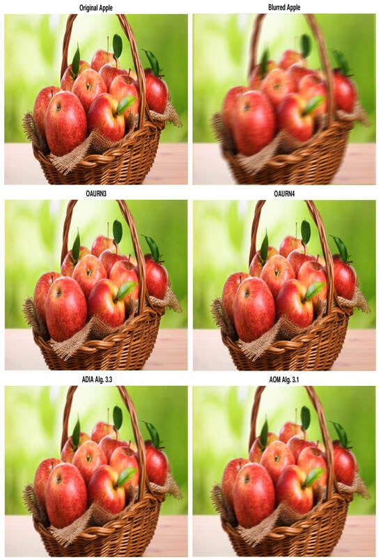
Figure 1. Comparison of restored images via various methods when the number of iterations is 2000 for the apple image.

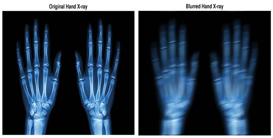
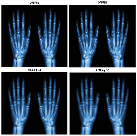
Figure 2. Comparison of restored images via various methods when the number of iterations is 2500 for the hand X-ray image.

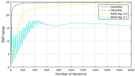
Figure 3. Graphs of SNR for the methods OAURN1, OAURN2, ADIA Alg. 3.3, and AOM Alg 3.1 for the apple image.

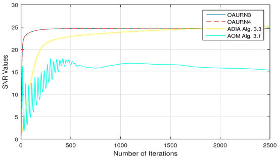
Figure 4. Graphs of SNR for the methods OAURN1, OAURN2, ADIA Alg. 3.3, and AOM Alg 3.1 for the Hand X-ray image.

Table 1. Numerical comparison for the methods OAURN1, OAURN2, ADIA Alg. 3.3, and AOM Alg. 3.1.

Images	k	OAURN1	OAURN2	ADIA Alg. 3.3	AOM Alg 3.1.
		SNR	SNR	SNR	SNR
Apple	300	23.8342	23.5978	20.8637	11.7830
Size = $350\times 600$	600	23.3478	23.04771	20.9999	11.9876
	1600	224.9893	24.5673	22.6738	16.3562
	2000	24.7839	24.3435	22.8246	16.8673
	300	23.9984	23.6374	21.2243	11.7803
Hand X-ray	600	23.9999	23.8563	21.6754	11.8587
Size = $520\times 750$	1600	24.9738	24.8973	22.7437	16.3478
	2500	24.99989	24.94555	22.5467	17.8495

Remark 4.

From Figure 1, Figure 2, Figure 3 and Figure 4 and Table 1, one can see that the qualities of the recovered images are better with higher SNR values. Thus, it is evident that Algorithms 1 and 2 are more efficient than the other compared algorithms.

5. Numerical Experiments

In this section, we present some numerical experiments to illustrate the numerical behavior of Algorithms 1 (in short, OAURN1) and 2 (in short, OAURN2). Moreover, we compare them with Algorithm 3.3 by Adamu et al. [36] (in short, ADIA Alg. 3.3) and Algorithm 3.1 by Alakoya et al. [15] (in short, AOM Alg. 3.1). We choose the parameters of all the methods as follows:

• In the proposed Algorithms 1 and 2, we set $\varphi =0.73$, ${\lambda }_1=2.5$, $s=0.59$, $c_1=0.67$, ${\vartheta }_k=0.89$, ${\alpha }_k=\frac{1}{2k+1}$, ${ϵ}_k=\frac{1}{{(2k+1)}^3}$, $s_k=\frac{1}{k+1}$, $\varrho =\frac{1.7\eta }{L_1^2}$ and $q_k=\frac{1}{{(k+1)}^{1.1}}$.
• In ADIA Alg. 3.3, we set ${\tau }_k=\frac{1}{2k+1}$, ${\sigma }_k={\mu }_k=0.5(1-{\tau }_k)$, ${ϵ}_k={\gamma }_k=s_k=\frac{1}{{(2k+1)}^2}$, $u=\frac{1}{2}$, ${\lambda }_k=\frac{1}{6}$ and $a=0.9$.
• In AOM Alg. 3.1, we set ${\alpha }_k=\frac{1}{2k+1}$, ${\delta }_k={\xi }_k=0.5(1-{\alpha }_k)$, ${ϵ}_k=\frac{1}{{(2k+1)}^3}$, $\theta =0.73$, ${\lambda }_1=2.5$, $\varphi =0.59$, $\alpha =0.145$, $\beta =0.465$, $Sp=\frac{2}{3}p$, $Tp=\frac{2}{3}p$, $f\left(p\right)=\frac{1}{2}p$ and ${\varphi }_k=\frac{1}{{(k+1)}^{1.1}}$.

Example 1.

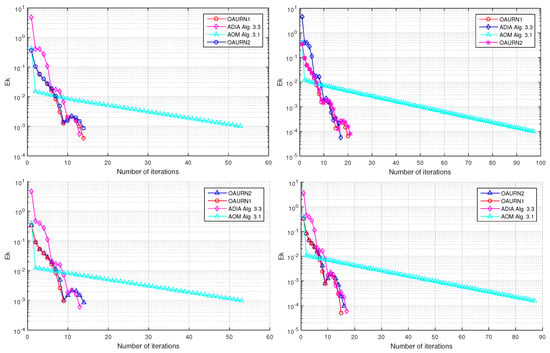
Let $\mathcal{H}=L_2\left([0,1]\right)$ and let the operators $D,E,F:\mathcal{H}\to \mathcal{H}$ be defined by

$$\begin{array}{c}\hfill D\left(p\right)=3p\left(t\right),E\left(p\right)=6p\left(t\right),\mathrm{and}\mathcal{F}\left(p\right)=0.5p\left(t\right),\forall t\in [0,1].\end{array}$$

It is not hard to verify that D is $\frac{1}{2}$-inverse strongly monotone, E is a maximal monotone operator, and $\mathcal{F}$ is $0.5$-strongly monotone and 0.5-Lipschitz continuous. For this experiment, we take the stopping $E_k=\parallel p_{k+1}-p_k\parallel <{10}^{-5}$ and consider the following cases:

• Case I: $p_0\left(t\right)=t$ and $p_1\left(t\right)=1+t^2$;
• Case II: $p_0\left(t\right)=2s$ and $p_1\left(t\right)=sin\left(t\right)$;
• Case III: $p_0\left(t\right)=t^3+t$ and $p_1\left(t\right)=t^3+3t$,
• Case IV: $p_0\left(t\right)=t+2$ and $p_1\left(t\right)=cos\left(t\right)$.

The obtained numerical results are presented in the following Table 2 and Figure 5. It can be seen that our method outperforms the compared methods.

Table 2. Numerical results of Example 1.

Cases		OAURN1	OAURN2	ADIA A1g. 3.3	AOM Alg. 3.1
Case I	CPU time (s)	0.0354	0.0385	0.058834	0.7367
	No. of Iter.	15	15	17	55
Case II	CPU time (s)	0.00456	0.005687	0.0864	0.2673
	No. of Iter.	15	15	18	98
Case III	CPU time (s)	0.0853	0.0987	0.1343	0.4536
	No. of Iter.	14	14	17	57
Case IV	CPU time (s)	0.1637	0.1856	0.35468	0.9637
	No. of Iter.	16 16	17	18	88

Figure 5. Example 1, Case I (top left); Case II (top right); Case III (bottom left); Case IV (bottom right).

Example 2.

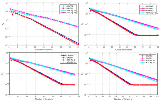
Let $H=({\mathcal{l}}_2\left(\mathbb{R}\right),\parallel ·{\parallel }_{{\mathcal{l}}_2})$, where ${\mathcal{l}}_2\left(\mathbb{R}\right)=\{p=(p_1,p_2,p_3,\cdots ),p_j\in \mathbb{R}:{\sum }_{j=1}^{\infty }\left|u_j\right|<\infty \}$ and ${\parallel p\parallel }_{{\mathcal{l}}_2}=({\sum }_{j=1}^{\infty }|p_j{{|}^2)}^{\frac{1}{2}}$, $\forall p\in {\mathcal{l}}_2\left(\mathbb{R}\right)$. We now define the operators $D,E,\mathcal{F}:{\mathcal{l}}_2\left(\mathbb{R}\right)\to {\mathcal{l}}_2\left(\mathbb{R}\right)$ by

$$\begin{array}{c}\hfill Dp=0.5p,Ep=8p,\mathrm{and}\mathcal{F}\left(p\right)=0.8p,\forall p\in \mathcal{H}.\end{array}$$

It is easy to check that D is 2-inverse strongly monotone, E is a maximal monotone operator, and $\mathcal{F}$ is $0.8$-strongly monotone and 0.8-Lipschitz continuous. For this experiment, we take the stopping $E_k=\parallel p_{k+1}-p_k\parallel <{10}^{-8}$ and consider the following cases:

• Case A: $p_0=\left(\frac{1}{4},\frac{1}{8},\frac{1}{9},\cdots \right)$ and $p_1=\left(1,\frac{1}{2},\frac{1}{3},\cdots \right)$.
• Case B: $p_0=\left(\frac{1}{5},\frac{1}{7},\frac{1}{10},\cdots \right)$ and $p_1=\left(1,\frac{1}{3},\frac{1}{5},\cdots \right)$.
• Case C: $p_0=\left(1,\frac{1}{8},\frac{1}{10},\cdots \right)$ and $p_1=\left(\frac{1}{6},\frac{1}{5},\frac{1}{7}\cdots \right)$.
• Case D: $p_0=\left(\frac{1}{2},\frac{1}{6},\frac{1}{8},\cdots \right)$ and $p_1=\left(1,\frac{1}{5},\frac{1}{10},\cdots \right)$.

The obtained numerical results are shown in Table 3 and Figure 6; it can be seen that our method outperformed the compared methods.

Table 3. Numerical results of Example 2.

Cases		OAURN1	OAURN2	ADIA Alg. 3.3	AOM Alg. 3.1
Case A	CPU time (s)	0.0060	0.0061	0.0099	0.0187
	No of Iter.	48	49	70	89
Case B	CPU time (s)	0.0073	0.0075	0.0167	0.0376
	No of Iter.	46	49	73	90
Case C	CPU time (s)	0.0038	0.0041	0.0562	0.0876
	No of Iter.	47	50	60	72
Case D	CPU time (s)	0.0052	0.0054	0.2536	0.4667
	No of Iter.	58	61	77	97

Figure 6. Example 2, Case A (top left); Case B (top right); Case C (bottom left); Case D (bottom right).

6. Conclusions

In this work, two efficient iterative methods for solving the strongly monotone variational inequality problem over the solution set of the monotone inclusion problem have been introduced. These methods are accelerated by the inertial technique. The new methods use self-adaptive step sizes rather than depending on prior knowledge of the operator norm and the Lipschitz constants of the operators involved. We obtained the strong convergence results of these methods under some mild conditions on the control parameters. We applied our results to solve the variational inequality problem, bilevel variational inequality problem, convex minimization problem, and image recovery problems. Numerical experiments were carried out to authenticate the applicability of our methods and to further show the superiority of the proposed method over some existing methods. The new results improve, extend, complement, and unify some existing results in [4,12,13,27] and several others.

References

- Abuchu, J.A.; Ofem, A.E.; Ugwunnadi, G.C.; Narain, O.K.; Hussain, A. Hybrid Alternated Inertial Projection and Contraction Algorithm for Solving Bilevel Variational Inequality Problems. J. Math. 2023, 2023, 3185746. [Google Scholar] [CrossRef]
- Ofem, A.E. Strong convergence of a multi-step implicit iterative scheme with errors for common fixed points of uniformly L–Lipschitzian total asymptotically strict pseudocontractive mappings. Results Nonlinear Anal. 2020, 3, 100–116. [Google Scholar]
- Ofem, A.E.; Mebawondu, A.A.; Ugwunnadi, G.C.; Işık, H.; Narain, O.K. A modified subgradient extragradient algorithm-type for solving quasimonotone variational inequality problems with applications. J. Inequal. Appl. 2023, 2023, 73. [Google Scholar] [CrossRef]
- Cholamjiak, P.; Hieu, D.V.; Cho, Y.J. Relaxed forward–backward splitting methods for solving variational inclusions and applications. J. Sci. Comput. 2021, 88, 85. [Google Scholar] [CrossRef]
- Gibali, A.; Thong, D.V. Tseng type methods for solving inclusion problems and its applications. Calcolo 2018, 55, 49. [Google Scholar] [CrossRef]
- Lions, P.L.; Mercier, B. Splitting algorithms for the sum of two nonlinear operators. SIAM J. Numer. Anal. 1979, 16, 964–979. [Google Scholar] [CrossRef]
- Ofem, A.E.; Mebawondu, A.A.; Ugwunnadi, G.C.; Cholamjiak, P.; Narain, O.K. Relaxed Tseng splitting method with double inertial steps for solving monotone inclusions and fixed point problems. Numer. Algor. 2023. [Google Scholar] [CrossRef]
- Ofem, A.E.; Işik, H.; Ali, F.; Ahmad, J. A new iterative approximation scheme for Reich–Suzuki type nonexpansive operators with an application. J. Inequal. Appl. 2022, 2022, 28. [Google Scholar] [CrossRef]
- Shehu, Y.; Dong, Q.L.; Jiang, D. Single projection method for pseudo-monotone variational inequality in Hilbert spaces. Optimization 2019, 68, 385–409. [Google Scholar] [CrossRef]
- Passty, G.B. Ergodic convergence to a zero of the sum of monotone operators in Hilbert space. J. Math. Anal. Appl. 1979, 72, 383–390. [Google Scholar] [CrossRef]
- Izuchukwu, C.; Reich, S.; Shehu, Y.; Taiwo, A. Strong Convergence of Forward-Reflected-Backward Splitting Methods for Solving Monotone Inclusions with Applications to Image Restoration and Optimal Control. J. Sci. Comput. 2023, 94, 73. [Google Scholar] [CrossRef]
- Tan, B.; Cho, S.Y. Strong Convergence of inertial forward-backward methods for solving monotone inclusions. Appl. Anal. 2022, 101, 5386–5414. [Google Scholar] [CrossRef]
- Tseng, P. A modified forward-backward splitting method for maximal monotone mappings. SIAM J. Control Optim. 2000, 38, 431–446. [Google Scholar] [CrossRef]
- Zhang, C.; Wang, Y. Proximal algorithm for solving monotone variational inclusion. Optimization 2018, 67, 1197–1209. [Google Scholar] [CrossRef]
- Alakoya, T.O.; Ogunsola, O.J.; Mewomo, O.T. An inertial viscosity algorithm for solving monotone variational inclusion and common fixed point problems of strict pseudocontractions. Bol. Soc. Mat. Mex. 2023, 29, 31. [Google Scholar] [CrossRef]
- Thong, D.V.; Anh, P.K.; Dung, V.T.; Linh, D.T.M. A Novel Method for Finding Minimum-norm Solutions to Pseudomonotone Variational Inequalities. Netw. Spat. Econ. 2023, 23, 39–64. [Google Scholar] [CrossRef]
- Polyak, B.T. Some methods of speeding up the convergence of iteration methods. USSR Comput. Math. Math. Phys. 1964, 4, 1–17. [Google Scholar] [CrossRef]
- Thong, D.V.; Hieu, D.V.; Rassias, T.M. Self adaptive inertial subgradient extragradient algorithms for solving pseudomonotone variational inequality problems. Optim. Lett. 2020, 14, 115–144. [Google Scholar] [CrossRef]
- Thong, D.V.; Liu, L.L.; Dong, Q.L.; Long, L.V.; Tuan, P.A. Fast relaxed inertial Tseng’s method-based algorithm for solving variational inequality and fixed point problems in Hilbert spaces. J. Comput. Appl. Math. 2023, 418, 114739. [Google Scholar] [CrossRef]
- Shehu, Y.; Yao, J.C. Rate of convergence for inertial iterative method for countable family of certain quasi–nonexpansive mappings. J. Nonlinear Convex Anal. 2020, 21, 533–541. [Google Scholar]
- Ofem, A.E.; Igbokwe, D.I. A new faster four step iterative algorithm for Suzuki generalized nonexpansive mappings with an application. Adv. Theory Nonlinear Anal. Its Appl. 2021, 5, 482–506. [Google Scholar]
- Ofem, A.E.; Abuchu, J.A.; George, R.; Ugwunnadi, G.C.; Narain, O.K. Some new results on convergence, weak w2–stability and data dependence of two multivalued almost contractive mappings in hyperbolic spaces. Mathematics 2022, 10, 3720. [Google Scholar] [CrossRef]
- Eslamian, M. Variational inequality over the solution set of split monotone variational inclusion problem with application to bilevel programming problem. Filomat 2023, 37, 8361–8376. [Google Scholar]
- Ofem, A.E.; Udofia, U.E.; Igbokwe, D.I. A robust iterative approach for solving nonlinear Volterra Delay integro-differential equations. Ural Math. J. 2021, 7, 59–85. [Google Scholar] [CrossRef]
- Okeke, G.A.; Ofem, A.E.; Abdeljawad, T.; Alqudah, M.A.; Khan, A. A solution of a nonlinear Volterra integral equation with delay via a faster iteration method. AIMS Math. 2023, 8, 102–124. [Google Scholar] [CrossRef]
- Yamada, I. The hybrid steepest decent method for variational inequality problem over intersection of fixed point sets of nonexpansive mapping. In Inherently Parallel Algorithm in Feasibility and Their Application; Butnariu, D., Censor, Y., Reich, S., Eds.; Elsevier: Amsterdam, The Netherlands, 2001; pp. 473–504. [Google Scholar]
- Lorenz, D.A.; Pock, T. An inertial forward–backward algorithm for monotone inclusions. Math. Imaging Vis. 2015, 51, 311–325. [Google Scholar] [CrossRef]
- Goebel, K.; Reich, S. Uniform Convexity, Hyperbolic Geometry, and Nonexpansive Mappings; Marcel Dekker: New York, NY, USA, 1984. [Google Scholar]
- Xu, H.K. Iterative algorithms for nonlinear operators. J. Lond. Math. Soc. 2002, 66, 240–256. [Google Scholar] [CrossRef]
- Brezis, H.; Chapitre, I.I. Operateurs maximaux monotones. North-Holland Math. Stud. 1973, 5, 19–51. [Google Scholar]
- Anh, P.K.; Anh, T.V.; Muu, L.D. On Bilevel split pseudomonotone variational inequality problems with applications. Acta Math. Vietnam. 2017, 42, 413–429. [Google Scholar] [CrossRef]
- Liu, H.; Yang, J. Weak convergence of iterative methods for solving quasimonotone variational inequalities. Comput. Optim. Appl. 2020, 77, 491–508. [Google Scholar] [CrossRef]
- Wang, Z.; Lei, Z.; Long, X.; Chen, Z. A modified Tseng splitting method with double inertial steps for solving monotone inclusion problems. J. Sci. Comput. 2023, 96, 92. [Google Scholar] [CrossRef]
- Kitkuan, D.; Kumam, P.; Martinez-Moreno, J. Generalized Halpern-type forward-backward splitting methods for convex minimization problems with application to image restoration problems. Optimization 2020, 69, 1–25. [Google Scholar] [CrossRef]
- Rockafellar, R. On the maximality of sums of nonlinear monotone operators. Trans. Amer. Math. Soc. 1970, 149, 75–88. [Google Scholar] [CrossRef]
- Adamu, A.; Deepho, J.; Ibrahim, A.H.; Abubakar, A.A.B. pproximation of zeros of sum of monotone mappings with applications to variational inequality and image restoration problems. Nonlinear Funct. Anal. Appl. 2021, 26, 411–432. [Google Scholar]
Disclaimer/Publisher’s Note: The statements, opinions and data contained in all publications are solely those of the individual author(s) and contributor(s) and not of MDPI and/or the editor(s). MDPI and/or the editor(s) disclaim responsibility for any injury to people or property resulting from any ideas, methods, instructions or products referred to in the content. |
© 2023 by the authors. Licensee MDPI, Basel, Switzerland. This article is an open access article distributed under the terms and conditions of the Creative Commons Attribution (CC BY) license (https://creativecommons.org/licenses/by/4.0/).