A General Iterative Procedure for Solving Nonsmooth Constrained Generalized Equations

Abstract

In this paper, we concentrate on an abstract iterative procedure for solving nonsmooth constrained generalized equations. This procedure employs both the property of weak point-based approximation and the approach of searching for a feasible inexact projection on the constrained set. Utilizing the contraction mapping principle, we establish higher order local convergence of the proposed method under the assumption of metric regularity property which ensures that the iterative procedure generates a sequence converging to a solution of the constrained generalized equation. Under strong metric regularity assumptions, we obtain that each sequence generated by this procedure converges to a solution. Furthermore, a restricted version of the proposed method is considered, for which we establish the desired convergence for each iterative sequence without a strong metric subregularity condition. The obtained results are new even for generalized equations without a constraint set.

1. Introduction and Background

Generalized equations are introduced by Robinson [1] with the following form:

$$f\left(x\right)+F\left(x\right)\ni 0,$$

(1)

where $f:X\to Y$ is a single-valued mapping and $F:X\rightrightarrows Y$ is a set-valued mapping between arbitrary Banach spaces. Model (1) as well as its various specifications have been widely recognized as a useful way to study optimization-related mathematical problems, such as linear and nonlinear complementarity problems, variational inequalities, first-order necessary conditions for nonlinear programming, equilibrium problems in both engineering and economics, etc.; see, e.g., [2,3,4,5,6] and the references therein. Specifically, it is called a variational system when F stands for the set of limiting subgradients. When we have F representing normal cone mapping associated with a closed convex set, it is called a variational inequality. For more details, please refer to [7,8] and the bibliographies therein.

To find an approximate solution to the generalized equation, there have been extensive studies of different versions of Newton’s method which are based on the assumption of strong metric regularity (cf. [9,10,11,12,13,14,15,16,17,18,19,20,21]). Newton’s method for unconstrained generalized Equation (1) dates back to Josephy [22], which is stated as follows. For the kth iterate $x_k\in X$, the $(k+1)$th iterate $x_{k+1}$ is computed according to the following inclusion:

$$f\left(x_k\right)+f^{\prime }\left(x_k\right)(x_{k+1}-x_k)+F\left(x_{k+1}\right)\ni 0,\mathrm{for}\mathrm{all}k\in \mathbb{N}$$

(2)

where $f^{\prime }$ represents the derivative of f. It simplifies to the regular version of Newton’s method for solving the nonlinear equation $f\left(x\right)=0$ when F is the zero mapping. When the single-valued mapping f is smooth, convergence rate results of Newton’s method (2) were established under the assumption that the partial linearization of the set-valued mapping $x\mapsto f\left(\overline{x}\right)+f^{\prime }\left(\overline{x}\right)(x-\overline{x})+F\left(x\right)$ is (strongly) metrically regular around $\overline{x}$ for 0, where $\overline{x}$ is the solution of (1). It is well understood that there exists a sequence generated by (2) which converges linearly if $f^{\prime }$ is continuous on a neighborhood of $\overline{x}$ and converges quadratically, provided that $f^{\prime }$ is Lipschitz continuous on a neighborhood of $\overline{x}$, respectively. When the function f in (2) is nonsmooth, we cannot use the usual method of partially linearizing on f anymore. In this situation, there are different ways of constructing abstract iterative procedures which are mainly based on the idea of point-based approximation (PBA). The concept of PBA was first developed by Robinson [23] and has been studied by many researchers. Geoffroy and Piétrus proposed in [24] a generalized concept of point-based approximation to generate an iterative procedure for generalized equations. The authors obtained convergence results on the nonsmooth Newton-type procedure which includes both local and semilocal versions (see [12,13,16,24,25,26] and the references therein).

Inexact Newton methods for solving smooth equation $f\left(x\right)=0$ in finite dimensions (i.e., (1) with $F\equiv 0$ and $X=Y={\mathbb{R}}^n$) were introduced by Dembo, Eisenstat, and Steihaug [27]. Specifically, for a given sequence $\left\{{\eta }_k\right\}\subset (0,+\infty )$ and a starting point $x_0$, the $(k+1)$th iterate is selected to satisfy the condition

$$(f\left(x_k\right)+f^{\prime }\left(x_k\right)(x_{k+1}-x_k))\cap B_{{\eta }_k\parallel f\left(x_k\right)\parallel }\left(0\right)\ne \varnothing ,$$

(3)

where $B_{{\eta }_k\parallel f\left(x_k\right)\parallel }\left(0\right)$ stands for the closed ball of radius ${\eta }_k\parallel f\left(x_k\right)\parallel$ centered at 0. For solving generalized Equation (1) in the Banach space setting, Dontchev and Rockafellar [15] proposed the following inexact Newton method:

$$(f\left(x_k\right)+f^{\prime }\left(x_k\right)(x_{k+1}-x_k)+F\left(x_{k+1}\right))\cap R_k(x_k,x_{k+1})\ne \varnothing ,\mathrm{for}\mathrm{all}k\in \mathbb{N}$$

(4)

where $R_k:X\times X\rightrightarrows Y$ is a sequence of set-valued mappings with closed graphs which represent the inexactness of the general model (1) and are not actually calculated in a specified manner. Under the metric regularity assumption, Dontchev and Rockafellar [15] show that the aforementioned method is executable and generate a sequence which converges either linearly, superlinearly, or quadratically.

In this paper, we focus on the study of a general iterative procedure for solving the nonsmooth constrained generalized equation

$$x\in C,f\left(x\right)+F\left(x\right)\ni 0,$$

(5)

where $\mathsf{\Omega }\subset {\mathbb{R}}^n$ is an open set, $C\subset \mathsf{\Omega }$ is a closed convex set, $f:\mathsf{\Omega }\to {\mathbb{R}}^m$ is a single-valued mapping which is not necessarily smooth, and $F:\mathsf{\Omega }\rightrightarrows {\mathbb{R}}^m$ is a closed set-valued mapping. Due to the presence of the constraint set C, constrained generalized Equation (5) can be viewed as an abstract model which covers several constrained optimization problems such as the Constrained Variational Inequality Problem, and, in particular, the Split Variational Inequality Problem. For more details about these problems, please refer to [28,29] and the references therein.

For solving the constrained generalized Equation (5) when f is smooth, Oliveira et al. [30] proposed a Newton’s method with feasible inexact projection (the Newton-InexP method). The procedure of incorporating a feasible inexact projection rectifies the shortcoming that, in standard Newton’s method (2), the next iterate $x_{k+1}$ may be infeasible for the constraint set C. Under the condition of metric regularity and assuming that the derivative $f^{\prime }$ is Lipschitz continuous, the authors in [30] established linear and quadratic convergence for the Newton-InexP method.

When the single-valued mapping f in the constrained generalized Equation (5) is not smooth, the partial linearization technique in the Newton-InexP approach in [30] is no longer applicable, and hence a new approach without involving the derivative of f is in demand. To this end, in this paper, we introduce a weak version of point-based approximation. For a class of single-valued functions which admit weak point-based approximations, we address a general inexact iterative procedure for solving (5) which incorporates a feasible inexact projection onto the constraint set. We aim to establish higher order convergence results for the proposed method assuming metric regularity on the weak point-based approximation of the mapping which generates the generalized equation. Taking into account the fact that in general metric regularity property cannot guarantee that every sequence generated with this method converges to a solution, we consider a restricted version of the aforementioned generalized procedure and establish convergence results for each iterative sequence accordingly.

The rest of this paper is structured in the following way. In Section 2, we provide the notations and a few technical results that we will use in the rest of the paper. In Section 3, we define the general iterative procedure for nonsmooth generalized Equation (5) and conduct local convergence analysis. Exact conditions are provided to ensure higher order convergence for this method as well as convergence for the arbitrary iterative sequence of a restricted version of the aforementioned procedure. In Section 5, we provide a numerical example to illustrate the assumptions and the local convergence result of the proposed approach.

2. Notation and Auxiliary Results

In this section, we display a few notations, definitions, and results that are utilized all through the paper. Let $\mathbb{N}=\{0,1,2,\cdots \}$. The symbol $B_{{\mathbb{R}}^n}$ stands for the closed unit ball of the space ${\mathbb{R}}^n$, while $B_r\left(x\right)$ indicates the closed ball of radius $r>0$ centered at $x\in {\mathbb{R}}^n$. Given subsets $C,D\subset {\mathbb{R}}^n$, define the distance from $x\in {\mathbb{R}}^n$ to C and the excess from C to D using

$$d(x,C):=inf\{\parallel x-c\parallel :c\in C\}\mathrm{and}e(C,D):=sup\left\{d\right(c,D):c\in C\},$$

(6)

respectively, with the convention that $d(x,\varnothing ):=\infty$, $e(\varnothing ,D):=0$ if $D\ne \varnothing$, and $e(\varnothing ,D):=\infty$ if $D=\varnothing$. Let $F:{\mathbb{R}}^n\rightrightarrows {\mathbb{R}}^m$ be a set-valued mapping and its graph be defined as

$$\mathrm{gph}\left(F\right):=\{(x,y)\in {\mathbb{R}}^n\times {\mathbb{R}}^m:y\in F\left(x\right)\}.$$

F is said to have a closed graph if the set $\mathrm{gph}\left(F\right)$ is closed in the product space ${\mathbb{R}}^n\times {\mathbb{R}}^m$. We use $F^{-1}:{\mathbb{R}}^m\rightrightarrows {\mathbb{R}}^n$ to represent the inverse mapping of F with $F^{-1}\left(y\right):=\{x\in {\mathbb{R}}^n:y\in F\left(x\right)\}$ for all $y\in {\mathbb{R}}^m$. For a single-valued mapping $g:X\to Y$, it is said to be Hölder calm at $\overline{x}\in X$ of order $p\ge 0$, if there exist constants $a,L>0$ such that

$$\parallel g\left(x\right)-g\left(\overline{x}\right)\parallel \le L\parallel x-\overline{x}{\parallel }^p,\forall x\in B_a\left(\overline{x}\right).$$

We say that g is Lipschitzian on $\mathsf{\Omega }\subset X$ with modulus L, if 

$$\parallel g\left(x\right)-g\left(x^{\prime }\right)\parallel \le L\parallel x-x^{\prime }\parallel ,\forall x,x^{\prime }\in \mathsf{\Omega }.$$

We first recall the concept of $(n,\alpha )$-point-based approximation (also called $(n,\alpha )$-PBA), which was introduced in [24].

Definition 1.

Let Ω be an open subset of a metric space $(X,d)$, Y be a normed linear space, and $f:\Omega \to Y$ be a single-valued mapping. Fix $n\in \mathbb{N}$ and $\alpha >0$. We say that the mapping $A:\Omega \times \Omega \to Y$ is an $(n,\alpha )$-PBA on Ω for f with modulus $\kappa >0$, if both of the following assertions hold:

(a) $\parallel f\left(v\right)-A(u,v)\parallel \le \frac{\kappa }{{\pi }_{n,\alpha }}{\parallel u-v\parallel }^{n+\alpha }$ for all $u,v\in \Omega$, where ${\pi }_{n,\alpha }:={\prod }_{i=1}^n(\alpha +i)$;

(b) The mapping $·\mapsto A(u,·)-A(v,·)$ is Lipschitzian on Ω with modulus ${\gamma \left(\kappa \right)\parallel u-v\parallel }^{\alpha }$, where $\gamma \left(\kappa \right)$ is a positive function of κ.

It is easy to see that when both n and $\alpha$ take the value of one in the above assertions, the $(1,1)$-PBA reduces to the PBA of f on $\mathsf{\Omega }$ according to Robinson [23]. In the nonsmooth framework, the normal maps are referred to as functions that have a (1,1)-PBA. For the smooth case, the authors showed in [24] that, if a function f is twice Fréchet differentiable on $\mathsf{\Omega }$ and satisfies that ${\nabla }^{2}f$ is $\mathrm{H}\ddot{\mathrm{o}}\mathrm{lder}$ with exponent $\alpha \in [0,1]$ and with constant $\kappa >0$, then it has a $(2,\alpha )$-PBA represented by $A(u,v)=f\left(u\right)+\nabla f\left(u\right)(v-u)+\frac{1}{2}{\nabla }^{2}f\left(u\right){(v-u)}^2$. For more details, please refer to the appendix in [24].

Next, we define the concept of $(n,\alpha )$-weak-point-based approximation for single-valued mappings at given points, which is essential in the generalized iterative procedure studied in Section 3.

Definition 2.

Let Ω be an open subset of a metric space $(X,d)$, Y be a normed linear space, and $f:\Omega \to Y$ be a single-valued mapping. Fix $n\in \mathbb{N}$ and $\alpha \ge 0$. We say that the mapping $A:\Omega \times \Omega \to Y$ is an $(n,\alpha )$-weak-point-based approximation ($(n,\alpha )$-WPBA) at $\overline{x}\in \Omega$ for f with modulus $\kappa >0$ and constant $a>0$, if both of the following assertions hold:

(a) $\parallel f\left(\overline{x}\right)-A(x,\overline{x})\parallel \le \frac{\kappa }{{\pi }_{n,\alpha }}{\parallel x-\overline{x}\parallel }^{n+\alpha }$ for all $x\in B_a\left(\overline{x}\right)$, where ${\pi }_{n,\alpha }:={\prod }_{i=1}^n(\alpha +i)$;

(b) For any $x\in B_a\left(\overline{x}\right)$, the mapping $·\mapsto A(\overline{x},·)-A(x,·)$ is Lipschitzian on Ω with modulus $\gamma \left(\kappa \right)\parallel x-\overline{x}{\parallel }^{\alpha }$, where $\gamma \left(\kappa \right)$ is a positive function of κ.

It is clear that the notion of $(n,\alpha )$-WPBA is weaker than the notion of $(n,\alpha )$-PBA. In the smooth setting, the authors proved in Lemma 3.1 of [31] that any continuously differentiable mapping f around $\overline{x}$ such that the derivative $f^{\prime }$ is Hölder calm (which is weaker than the Lipschitz continuity) of order $\alpha \ge 0$ admits a $(1,\alpha )$-PBA given by $A(x,u)=f\left(x\right)+f^{\prime }\left(x\right)(u-x)$. Let us observe that relation $\left(a\right)$ implies in particular that $A(\overline{x},\overline{x})=f\left(\overline{x}\right)$.

In the following, we present the definition of (strong) metric regularity, which plays an important role in our later analysis.

Definition 3.

Let $\kappa ,a,b>0$, $F:{\mathbb{R}}^n\rightrightarrows {\mathbb{R}}^m$ be a set-valued mapping and $(\overline{x},\overline{y})\in \mathrm{gph}\left(F\right)$. F is said to be metrically regular at $\overline{x}$ for $\overline{y}$ with constants $\kappa ,a$, and b, if 

$$d(x,F^{-1}\left(y\right))\le \kappa d(y,F\left(x\right)),\mathrm{for}\mathrm{all}x\in B_a\left(\overline{x}\right)andy\in B_b\left(\overline{y}\right).$$

(7)

F is said to be strongly metrically regular at $\overline{x}$ for $\overline{y}$ with constants $\kappa ,a$, and b, if (7) holds and $F^{-1}\left(y\right)\cap B_a\left(\overline{x}\right)$ is singleton for each $y\in B_b\left(\overline{y}\right)$.

It is widely understood that F is strongly metrically regular at $\overline{x}$ for $\overline{y}$ with constants $\kappa ,a$, and b if and only if the mapping $B_b\left(\overline{y}\right)\ni y\mapsto F^{-1}\left(y\right)\cap B_a\left(\overline{x}\right)$ is single-valued and Lipschitz continuous on $B_b\left(\overline{y}\right)$; for more details, see [7]. If $f:{\mathbb{R}}^n\to {\mathbb{R}}^m$ is smooth around $\overline{x}\in {\mathbb{R}}^n$, then f is strongly metrically regular at $\overline{x}$ for $f\left(\overline{x}\right)$ if and only if $f^{\prime }\left(\overline{x}\right)$ is invertible.

In [30], the authors introduced the following concept of feasible inexact projection, which is the basic structure of the Newton-InexP method studied therein.

Definition 4.

Let $C\subset {\mathbb{R}}^n$ be a closed convex set, $x\in C$, and $\theta \ge 0$. The feasible inexact projection mapping relative to x with error tolerance θ is denoted by $P_C(·,x,\theta ):{\mathbb{R}}^n\rightrightarrows C$. The definition is as follows:

$$P_C{(u,x,\theta ):=\{w\in C:⟨u-w,z-w⟩\le \theta \parallel u-x\parallel }^2,\forall z\in C\},forallu\in {\mathbb{R}}^n.$$

Any element $w\in P_C(u,x,\theta )$ is said to be a feasible inexact projection of u onto C with respect to x and with error tolerance θ.

Since $C\subset {\mathbb{R}}^n$ is a closed convex set, Proposition 2.1.3 of [32] implies that for each $u\in {\mathbb{R}}^n$ and $x\in C$, we have $P_C\left(u\right)\in P_C(u,x,\theta )$ and $\left\{P_C\left(u\right)\right\}=P_C(u,x,0)$, where $P_C$ denotes the exact projection mapping (see Remark 2 of [30]). In particular, the point $w\in P_C(u,x,\theta )$ is an approximate feasible solution for the projection subproblem ${min}_{z\in C}{\parallel z-u\parallel }^2/2$, which satisfies $⟨u-w,z-w⟩\le {\theta \parallel u-x\parallel }^2$ for all $z\in C$.

The next result, Lemma 1 of [30], is useful in the remainder of this paper.

Lemma 1.

Let $y,\tilde{y}\in {\mathbb{R}}^n$, $x,\tilde{x}\in C$, and $\theta \ge 0$. Then, for any $w\in P_C(y,x,\theta )$, we have

$$\parallel P_C(\tilde{y},\tilde{x},0)-w\parallel \le \parallel y-\tilde{y}\parallel +\sqrt{2\theta }\parallel y-x\parallel .$$

We end this section by recalling the well-known contraction mapping principle for set-valued mappings (see Theorem 5E.2 of [7]).

Lemma 2.

Let $\mathsf{\Phi }:X\rightrightarrows X$ be a set-valued mapping defined on a complete metric space X, $\overline{x}\in X$, and let $r>0$ be such that the set $\mathrm{gph}\left(\mathsf{\Phi }\right)\cap B_r\left(\overline{x}\right)\times B_r\left(\overline{x}\right)$ is closed in $X\times X$. Given $\alpha \in (0,1)$, impose the following assumptions:

1. 

$d(\overline{x},\mathsf{\Phi }\left(\overline{x}\right))<r(1-\alpha )$.

2. 

$e(\mathsf{\Phi }\left(u\right)\cap B_r\left(\overline{x}\right),\mathsf{\Phi }\left(v\right))\le \alpha d(u,v)forallu,v\in B_r\left(\overline{x}\right)$.

Then, Φ has a fixed point in $B_r\left(\overline{x}\right)$, i.e., there exists $x\in B_r\left(\overline{x}\right)$ such that $x\in \mathsf{\Phi }\left(x\right)$. In addition, if Φ is single-valued, then Φ has a unique fixed point in $B_r\left(\overline{x}\right)$.

3. Convergence Analysis

In this section, employing the notions of $(n,\alpha )$-WPBA and the feasible inexact projection defined in Section 2, we propose a general iterative procedure for solving nonsmooth constrained generalized Equation (5).

Let $\overline{x}\in C$ be such that $f\left(\overline{x}\right)+F\left(\overline{x}\right)\ni 0$ and $A:\mathsf{\Omega }\times \mathsf{\Omega }\to {\mathbb{R}}^m$ be an $(n,\alpha )$-WPBA at $\overline{x}$ for f. To formulize the iterative procedure, we choose $x_0\in C$, $\left\{{\theta }_k\right\}\subset [0,+\infty )$ as the input data and $R_k:{\mathbb{R}}^n\rightrightarrows {\mathbb{R}}^m$ for $k=0,1,2,\cdots$ as the inexactness (Algorithm 1).

Algorithm 1 General inexact projection method

Step 0. Let $x_0\in C$ and $\left\{{\theta }_j\right\}\subset [0,+\infty )$ be given, and set $k=0$. Step 1. If $f\left(x_k\right)+F\left(x_k\right)\ni 0$, then stop; otherwise, compute $u_k\in {\mathbb{R}}^n$ such that $$(A(x_k,u_k)+F\left(u_k\right))\cap R_k\left(x_k\right)\ne \varnothing .$$ (8) Step 2. If $u_k\in C$, set $x_{k+1}=u_k$; otherwise, take any $x_{k+1}$ satisfying $$x_{k+1}\in P_C(u_k,x_k,{\theta }_k).$$ (9) Step 3. Set $k\leftarrow k+1$, and go to Step 1.

Note that in comparison with (4), the mapping $R_k$ in Step 1 which represents inexactness now depends on the current iteration $x_k$ only. In Step 2, we utilize the weak point-based approximation of f in place of the linearization technique for the smooth case applied in [30]. In Step 3, the symbol $P_C(y_k,x_k,{\theta }_k)$ represents $y_k$’s feasible inexact projections onto C relative to $x_k$ with error tolerance ${\theta }_k$.

To conduct convergence analysis for the proposed method, for each fixed $x\in \mathsf{\Omega }$, we need to define the auxiliary mapping $g_x:\mathsf{\Omega }\to {\mathbb{R}}^m$:

$$g_x\left(u\right):=A(\overline{x},u)-A(x,u),\forall u\in \mathsf{\Omega }.$$

(10)

For convenience, we define $L_x:\mathsf{\Omega }\rightrightarrows {\mathbb{R}}^m$ as the approximation of the set-valued mapping $f+F$:

$$L_x\left(u\right):=A(x,u)+F\left(u\right),\forall u\in \mathsf{\Omega }.$$

(11)

We analyze based on the assumption that an approximation of the set-valued mapping $f+F$ ensures metric regularity/strong metric regularity, and that f has weak point-based approximation which is weaker than the condition of point-based approximation.

To prove our main result, we will first explain some technical results that will be helpful in our later analysis. The following Lemma can be shown with some simple calculations.

Lemma 3.

Let $\alpha \ge 0$, $\kappa ,a>0,n\in \mathbb{N}$, and $f:\Omega \to {\mathbb{R}}^m$ be a single-valued mapping. Assume that $A:\Omega \times \Omega \to {\mathbb{R}}^m$ is an $(n,\alpha )$-WPBA at $\overline{x}$ for f with modulus κ and constant a. Then,

$$\parallel g_x\left(u\right)-g_x\left(u^{\prime }\right)\parallel \le \gamma \left(\kappa \right)\parallel x-\overline{x}{\parallel }^{\alpha }\parallel u-u^{\prime }\parallel ,\forall x\in B_a\left(\overline{x}\right),u,u^{\prime }\in \mathsf{\Omega }$$

(12)

and

$$\parallel g_x\left(u\right)\parallel \le \frac{\kappa }{{\pi }_{n,\alpha }}\parallel x-\overline{x}{\parallel }^{n+\alpha }+\gamma \left(\kappa \right)\parallel x-\overline{x}{\parallel }^{\alpha }\parallel u-\overline{x}\parallel ,\forall x\in B_a\left(\overline{x}\right),u\in \mathsf{\Omega }.$$

(13)

Proof. 

Since A is an $(n,\alpha )$-WPBA at $\overline{x}$ for f with modulus $\kappa$ and constant a, we have

$$\begin{array}{cc}\hfill \parallel g_x\left(u\right)-g_x\left(u^{\prime }\right)\parallel & =\parallel A(\overline{x},u)-A(x,u)-(A(\overline{x},u^{\prime })-A(x,u^{\prime }))\parallel \hfill \\ & \le \gamma \left(\kappa \right)\parallel x-\overline{x}{\parallel }^{\alpha }\parallel u-u^{\prime }\parallel ,\forall x\in B_a\left(\overline{x}\right),u,u^{\prime }\in \mathsf{\Omega }.\hfill \end{array}$$

Note that $f\left(\overline{x}\right)=A(\overline{x},\overline{x})$ for any fixed $x\in B_a\left(\overline{x}\right)$ and $u\in \mathsf{\Omega }$, one has

$$\begin{array}{cc}\hfill \parallel g_x\left(u\right)\parallel & =\parallel A(\overline{x},u)-A(x,u)\parallel \hfill \\ & \le \parallel f\left(\overline{x}\right)-A(x,\overline{x})\parallel +\parallel A(\overline{x},u)-A(x,u)-(A(\overline{x},\overline{x})-A(x,\overline{x}))\parallel \hfill \\ & \le \frac{\kappa }{{\pi }_{n,\alpha }}\parallel x-\overline{x}{\parallel }^{n+\alpha }+\gamma \left(\kappa \right)\parallel x-\overline{x}{\parallel }^{\alpha }\parallel u-\overline{x}\parallel \hfill \end{array}$$

which establishes (12) and (13).    □

Pick $x\in \mathsf{\Omega }$, $v\in {\mathbb{R}}^m$ and let them be fixed. For convenience, we define the following auxiliary set-valued mapping:

$${\mathsf{\Phi }}_{x,v}\left(u\right):=L_{\overline{x}}^{-1}(g_x\left(u\right)+v),\forall u\in X,$$

(14)

where $L_{\overline{x}}^{-1}\left(y\right):=\{u\in X:y\in L_{\overline{x}}\left(u\right)\}$ denotes the inverse of $L_{\overline{x}}$ defined as in (11). It is easy to observe that $u\in {\mathsf{\Phi }}_{x,v}\left(u\right)$ if and only if $x,u$, and v satisfy

$$A(x,u)+F\left(u\right)\ni v.$$

Lemma 4.

Assume that the assumptions in Lemma 3 hold. Let $\eta ,\tau ,b,r_{*}\in (0,+\infty )$ be such that

$$r_{*}\le a,\tau \gamma \left(\kappa \right)r_{*}^{\alpha }<1,\frac{(\kappa +\eta {\pi }_{n,\alpha })\tau r_{*}^{n+\alpha }}{{\pi }_{n,\alpha }(1-\tau \gamma \left(\kappa \right)r_{*}^{\alpha })}<r_{*}\mathit{and}\frac{(\kappa +\eta )r_{*}^{n+\alpha }}{{\pi }_{n,\alpha }}+\gamma \left(\kappa \right)r_{*}^{1+\alpha }\le b.$$

(15)

If $L_{\overline{x}}$ is metrically regular at $\overline{x}$ for 0 with constants $\tau ,a$, and b, then for any $x\in B_{r_{*}}\left(\overline{x}\right)$ and $v\in \eta r_{*}^{n+\alpha }{B}_{{\mathbb{R}}^m}$, there exists a fixed point $\overline{u}\in {\mathsf{\Phi }}_{x,v}\left(\overline{u}\right)$ such that

$$\parallel \overline{u}-\overline{x}\parallel \le \frac{\kappa \tau \parallel x-\overline{x}{\parallel }^{n+\alpha }+{\pi }_{n,\alpha }\tau \parallel v\parallel }{{\pi }_{n,\alpha }(1-\tau \gamma \left(\kappa \right)\parallel x-\overline{x}{\parallel }^{\alpha })}.$$

(16)

In particular, $\overline{u}\in B_{r_{*}}\left(\overline{x}\right)$. In addition, if the mapping $L_{\overline{x}}$ is strongly metrically regular at $\overline{x}$ for 0, then the mapping ${\mathsf{\Phi }}_{x,v}$ has exactly one fixed point in $B_{r_{*}}\left(\overline{x}\right)$ such that (16) holds.

Proof. 

Pick any $x\in B_{r_{*}}\left(\overline{x}\right)$ and $v\in \eta r_{*}^{n+\alpha }{B}_{{\mathbb{R}}^m}$. Let

$$\rho :=\frac{\kappa \tau \parallel x-\overline{x}{\parallel }^{n+\alpha }+{\pi }_{n,\alpha }\tau \parallel v\parallel }{{\pi }_{n,\alpha }(1-\tau \gamma \left(\kappa \right)\parallel x-\overline{x}{\parallel }^{\alpha })}.$$

(17)

It is easy to obtain from the choice of the constants that

$$\tau \gamma \left(\kappa \right)\parallel x-\overline{x}{\parallel }^{\alpha }\le \tau \gamma \left(\kappa \right)r_{*}^{\alpha }<1$$

and

$$\rho \le \frac{(\kappa +\eta {\pi }_{n,\alpha })\tau r_{*}^{n+\alpha }}{{\pi }_{n,\alpha }(1-\tau \gamma \left(\kappa \right)r_{*}^{\alpha })}\le r_{*}\le a.$$

Recall that $L_{\overline{x}}$ is metrically regular at $\overline{x}$ for 0 with constants $\tau ,a$, and b. We have

$$d(x,L_{\overline{x}}^{-1}\left(y\right))\le \tau d(y,L_{\overline{x}}\left(x\right))\forall (x,y)\in B_a\left(\overline{x}\right)\times B_b\left(0\right)$$

(18)

which indicates that $L_{\overline{x}}^{-1}\left(y\right)\ne \varnothing$ for any $y\in B_b\left(0\right)$. By (13) and (15), we have

$$\parallel g_x\left(\overline{x}\right)\parallel \le \frac{\kappa }{{\pi }_{n,\alpha }}{\parallel x-\overline{x}\parallel }^{n+\alpha }$$

(19)

and

$$\parallel g_x\left(u\right)+v\parallel \le \frac{\kappa }{{\pi }_{n,\alpha }}{r}_{*}^{n+\alpha }+\gamma \left(\kappa \right)r_{*}^{1+\alpha }+\parallel v\parallel \le b,\forall u\in B_{r_{*}}\left(\overline{x}\right).$$

(20)

Then, ${\mathsf{\Phi }}_{x,v}$ is well-defined on $B_{r_{*}}\left(\overline{x}\right)\subset B_a\left(\overline{x}\right)$. Since $0\in L_{\overline{x}}\left(\overline{x}\right)$, it follows from (17)–(19) that

$$\begin{array}{cc}\hfill d(\overline{x},{\mathsf{\Phi }}_{x,v}\left(\overline{x}\right))& =d(\overline{x},L_{\overline{x}}^{-1}(g_x\left(\overline{x}\right)+v))\hfill \\ & \le \tau d(g_x\left(\overline{x}\right)+v,L_{\overline{x}}\left(\overline{x}\right))\le \tau \parallel g_x\left(\overline{x}\right)+v\parallel \hfill \\ & \le \frac{\kappa \tau }{{\pi }_{n,\alpha }}\parallel x-\overline{x}{\parallel }^{n+\alpha }+\tau \parallel v\parallel =\rho (1-\tau \gamma \left(\kappa \right)\parallel x-\overline{x}{\parallel }^{\alpha }).\hfill \end{array}$$

(21)

Furthermore, it follows from (12) and (18) that

$$\begin{array}{cc}\hfill e({\mathsf{\Phi }}_{x,v}\left(u^{\prime }\right)& \cap B_{\rho }\left(\overline{x}\right),{\mathsf{\Phi }}_{x,v}\left(u\right))=sup\{d(y,{\mathsf{\Phi }}_{x,v}\left(u\right)):y\in {\mathsf{\Phi }}_{x,v}\left(u^{\prime }\right)\cap B_{\rho }\left(\overline{x}\right)\}\hfill \\ & \le \tau sup\{d(g_x\left(u\right)+v,L_{\overline{x}}\left(y\right)):y\in B_{\rho }\left(\overline{x}\right),g_x\left(u^{\prime }\right)+v\in L_{\overline{x}}\left(y\right)\}\hfill \\ & \le \tau \parallel g_x\left(u\right)-g_x\left(u^{\prime }\right)\parallel \le \tau \gamma \left(\kappa \right)\parallel x-\overline{x}{\parallel }^{\alpha }\parallel u^{\prime }-u\parallel \hfill \end{array}$$

(22)

holds for all $u^{\prime },u\in B_{\rho }\left(\overline{x}\right)$. Note that $\tau \gamma \left(\kappa \right)\parallel x-\overline{x}{\parallel }^{\alpha }<1$ and $B_{\rho }\left(\overline{x}\right)\subset B_a\left(\overline{x}\right)$, and applying Lemma 2 with $\mathsf{\Phi }={\mathsf{\Phi }}_{x,v},\overline{x}=\overline{x},r=\rho$, and $\alpha =\tau \gamma \left(\kappa \right)\parallel x-\overline{x}{\parallel }^{\alpha }$ ensures the existence of $\overline{u}\in {\mathsf{\Phi }}_{x,v}\left(\overline{u}\right)\cap B_{\rho }\left(\overline{x}\right)$, i.e., inequality (16) holds with $\overline{u}\in {\mathsf{\Phi }}_{x,v}\left(\overline{u}\right)$. Due to the fact that $\parallel \overline{u}-\overline{x}\parallel \le \rho \le r_{*}$, we arrive at $\overline{u}\in B_{r_{*}}\left(\overline{x}\right)$.

Next, we assume that the mapping $L_{\overline{x}}$ is strongly metrically regular at $\overline{x}$ for 0. Then, the mapping $B_b\left(0\right)\ni y:\mapsto L_{\overline{x}}^{-1}\left(y\right)\cap B_a\left(\overline{x}\right)$ is single-valued, and thus the mapping $B_{r_{*}}\left(\overline{x}\right)\ni u:\mapsto {\mathsf{\Phi }}_{x,v}{|}_{B_a\left(\overline{x}\right)}\left(u\right):={\mathsf{\Phi }}_{x,v}\left(u\right)\cap B_a\left(\overline{x}\right)$ is single-valued (thanks to (20)). Similar to the proofs of (21) and (22), we have

$$d(\overline{x},{\mathsf{\Phi }}_{x,v}{|}_{B_a\left(\overline{x}\right)}\left(\overline{x}\right))\le \rho (1-\tau \gamma \left(\kappa \right)\parallel x-\overline{x}{\parallel }^{\alpha })\le r_{*}(1-\tau \gamma \left(\kappa \right)\parallel x-\overline{x}{\parallel }^{\alpha })$$

and

$$d({\mathsf{\Phi }}_{x,v}{|}_{B_a\left(\overline{x}\right)}\left(u^{\prime }\right),{\mathsf{\Phi }}_{x,v}{|}_{B_a\left(\overline{x}\right)}\left(u\right))\le \tau \gamma \left(\kappa \right)\parallel x-\overline{x}{\parallel }^{\alpha }\parallel u^{\prime }-u\parallel ,\forall u^{\prime },u\in B_{r_{*}}\left(\overline{x}\right).$$

It follows from Lemma 2 (2) that ${\mathsf{\Phi }}_{x,v}{|}_{B_a\left(\overline{x}\right)}$ has a unique fixed point in $B_{r_{*}}\left(\overline{x}\right)$. Besides, since $B_{r_{*}}\left(\overline{x}\right)\subset B_a\left(\overline{x}\right)$, ${\mathsf{\Phi }}_{x,v}$ has a unique fixed point in $B_{r_{*}}\left(\overline{x}\right)$. By the first part of the proof, we know that ${\mathsf{\Phi }}_{x,v}$ has a fixed point $\overline{u}\in B_{\rho }\left(\overline{x}\right)\subset B_{r_{*}}\left(\overline{x}\right)$ satisfying (16); hence, $\overline{u}$ is the unique fixed point of ${\mathsf{\Phi }}_{x,v}$ in $B_{r_{*}}\left(\overline{x}\right)$, which completes the proof.    □

The following Lemma shows that there exists a unique solution in $B_{r_{*}}\left(\overline{x}\right)$ for generalized Equation (1) under the strong metric regularity assumption.

Lemma 5.

Let the assumptions in Lemmas 3 and 4 hold. If the mapping $L_{\overline{x}}$ is strongly metrically regular at $\overline{x}$ for 0 with constants $\tau ,a$, and b, then $\overline{x}$ is the unique solution of (1) in $B_{r_{*}}\left(\overline{x}\right)$.

Proof. 

Let $\widehat{x}$ be a solution of (1) in $B_{r_{*}}\left(\overline{x}\right)$. Since A is an $(n,\alpha )$-WPBA for f, we have

$$\parallel f\left(\widehat{x}\right)-A(\overline{x},\widehat{x})\parallel \le \frac{\kappa }{{\pi }_{n,\alpha }}{\parallel \widehat{x}-\overline{x}\parallel }^{n+\alpha }<\frac{\kappa r_{*}^{n+\alpha }}{{\pi }_{n,\alpha }}\le b.$$

(23)

Recall that $L_{\overline{x}}$ is strongly metrically regular at $\overline{x}$ for 0 with constants $\tau ,a$, and b. The mapping $y\mapsto L_{\overline{x}}\left(y\right)\cap B_a\left(\overline{x}\right)$ is single-valued on $B_b\left(0\right)$ and (18) holds. Furthermore, we know that

$$0\in f\left(\widehat{x}\right)+F\left(\widehat{x}\right)=f\left(\widehat{x}\right)-A(\overline{x},\widehat{x})+L_{\overline{x}}\left(\widehat{x}\right).$$

Hence, we conclude that

$$\widehat{x}=L_{\overline{x}}^{-1}(A(\overline{x},\widehat{x})-f\left(\widehat{x}\right))\cap B_a\left(\overline{x}\right).$$

Note that $0\in L_{\overline{x}}\left(\overline{x}\right)$. By (18) and (23), one has

$$\begin{array}{cc}\hfill \parallel \overline{x}-\widehat{x}\parallel & =d(\overline{x},L_{\overline{x}}^{-1}(A(\overline{x},\widehat{x})-f\left(\widehat{x}\right))\hfill \\ & \le \tau d(A(\overline{x},\widehat{x})-f\left(\widehat{x}\right),L_{\overline{x}}\left(\overline{x}\right))\hfill \\ & \le \tau \parallel A(\overline{x},\widehat{x})-f\left(\widehat{x}\right)\parallel \hfill \\ & \le \frac{\tau \kappa }{{\pi }_{n,\alpha }}{\parallel \widehat{x}-\overline{x}\parallel }^{n+\alpha }.\hfill \end{array}$$

Since $\frac{\tau \kappa }{{\pi }_{n,\alpha }}{\parallel \widehat{x}-\overline{x}\parallel }^{n+\alpha -1}\le \frac{\tau \kappa r_{*}^{n+\alpha -1}}{{\pi }_{n,\alpha }}<1$ (thanks to the third inequality in (15)), then $\parallel \widehat{x}-\overline{x}\parallel =0$. Hence, $\overline{x}$ is the unique solution of (1) in $B_{r_{*}}\left(\overline{x}\right)$.    □

The next Lemma plays an important role in the convergence analysis, the proof of which follows from the lines of Lemma 4 of [30].

Lemma 6.

Let the assumptions in Lemma 4 hold and $\theta \ge 0$. If $x\in B_{r_{*}}\left(\overline{x}\right)\setminus \left\{\overline{x}\right\}$ and $u\in {\mathsf{\Phi }}_{x,v}\left(u\right)$ satisfies (16), then, for any $w\in P_C(u,x,\theta )$, we have

$$\parallel w-\overline{x}\parallel \le \left(1+\sqrt{2\theta }\right)\frac{\kappa \tau \parallel x-\overline{x}{\parallel }^{n+\alpha }+{\pi }_{n,\alpha }\tau \parallel v\parallel }{{\pi }_{n,\alpha }(1-\tau \gamma \left(\kappa \right)\parallel x-\overline{x}{\parallel }^{\alpha })}+\sqrt{2\theta }\parallel x-\overline{x}\parallel .$$

(24)

Proof. 

Pick any $w\in P_C(u,x,\theta )$. Then, applying Lemma 1 with $\tilde{y}=\tilde{x}=\overline{x}$, we have

$$\parallel P_C(\overline{x},\overline{x},0)-w\parallel \le \parallel u-\overline{x}\parallel +\sqrt{2\theta }\parallel x-u\parallel \le \parallel u-\overline{x}\parallel +\sqrt{2\theta }(\parallel x-\overline{x}\parallel +\parallel u-\overline{x}\parallel ).$$

Note that $x\in B_{r_{*}}\left(\overline{x}\right)$ and $P_C(\overline{x},\overline{x},0)=\overline{x}$. It follows from (16) that

$$\parallel w-\overline{x}\parallel \le \left(1+\sqrt{2\theta }\right)\frac{\kappa \tau \parallel x-\overline{x}{\parallel }^{n+\alpha }+{\pi }_{n,\alpha }\tau \parallel v\parallel }{{\pi }_{n,\alpha }(1-\tau \gamma \left(\kappa \right)\parallel x-\overline{x}{\parallel }^{\alpha })}+\sqrt{2\theta }\parallel x-\overline{x}\parallel ,$$

which establishes (24).    □

Now, we are ready to present our main result. We derive the exact relationship between the rate of convergence of the proposed method and the constant of the weak point-based approximation.

Theorem 1.

Consider the nonsmooth constrained generalized Equation (5). Let $r:=sup\{t\in \mathbb{R}:B_t\left(\overline{x}\right)\subset \mathsf{\Omega }\}$, $\left\{{\theta }_k\right\}\subset [0,1/2)$, $\tilde{\theta }:={sup}_k{\theta }_k<\frac{1}{2}$; and $\alpha \ge 0$, $\kappa ,\tau ,\eta ,a,b,r_{*}>0$, which satisfy (15) and

$$r_{*}<r,\frac{\left(1+\sqrt{2\tilde{\theta }}\right)\left(\kappa +\eta {\pi }_{n,\alpha }\right)\tau r_{*}^{n+\alpha -1}}{{\pi }_{n,\alpha }(1-\tau \gamma \left(\kappa \right)r_{*}^{\alpha })}+\sqrt{2\tilde{\theta }}<1.$$

(25)

Assume that $\overline{x}\in C$ with $f\left(\overline{x}\right)+F\left(\overline{x}\right)\ni 0$, the set-valued mapping $L_{\overline{x}}$ is metrically regular at $\overline{x}$ for 0 with constants $\tau ,a$, and b, and the function $A:\Omega \times \Omega \to {\mathbb{R}}^m$ is an $(n,\alpha )$-WPBA at $\overline{x}$ for f with modulus κ and constant a. Furthermore, suppose that the sequence of set-valued mappings $\left\{R_k\right\}$ satisfies

$$\underset{k\in \mathbb{N}}{sup}\underset{v\in R_k\left(x\right)}{sup}\parallel v\parallel \le \eta \parallel x-\overline{x}{\parallel }^{n+\alpha },\forall x\in B_a\left(\overline{x}\right).$$

(26)

Then, for every starting point $x_0\in C\cap B_{r_{*}}\left(\overline{x}\right)\setminus \left\{\overline{x}\right\}$, there exists a sequence $\left\{x_k\right\}$ generated by the general inexact projection method associated with $\left\{{\theta }_k\right\}$ and $\left\{R_k\right\}$, which is contained in $C\cap B_{r_{*}}\left(\overline{x}\right)$ and converges to $\overline{x}$ with the following condition:

$$\parallel x_{k+1}-\overline{x}\parallel \le \left[\frac{\left(1+\sqrt{2{\theta }_k}\right)\left(\kappa +\eta {\pi }_{n,\alpha }\right)\tau {\parallel x_k-\overline{x}\parallel }^{n+\alpha -1}}{{\pi }_{n,\alpha }\left(1-\tau \gamma \left(\kappa \right)\parallel x_k-\overline{x}{\parallel }^{\alpha }\right)}+\sqrt{2{\theta }_k}\right]\parallel x_k-\overline{x}\parallel ,\forall k\in \mathbb{N}.$$

(27)

In particular, if ${\theta }_k=0$ for all $k=0,1,2,\dots$, then

$$\parallel x_{k+1}-\overline{x}\parallel \le \frac{\left(\kappa +\eta {\pi }_{n,\alpha }\right)\tau }{{\pi }_{n,\alpha }\left(1-\tau \gamma \left(\kappa \right)r_{*}^{\alpha }\right)}{\parallel x_k-\overline{x}\parallel }^{n+\alpha },\forall k\in \mathbb{N}$$

(28)

and $\left\{x_k\right\}$ converges to $\overline{x}$ superlinearly of order $n+\alpha$. Furthermore, if the mapping $L_{\overline{x}}$ is strongly metrically regular at $\overline{x}$ for 0, then $\overline{x}$ is the unique solution of (5) in $B_{r_{*}}\left(\overline{x}\right)$, and every sequence generated by the general inexact projection method starting at $x_0\in C\cap B_{r_{*}}\left(\overline{x}\right)\setminus \left\{\overline{x}\right\}$ which is contained in $B_{r_{*}}\left(\overline{x}\right)$ and associated with $\left\{{\theta }_k\right\},\left\{R_k\right\}$ satisfies (27) and converges to $\overline{x}$.

Proof. 

First, we will show by induction on k that, for any starting point $x_0\in C\cap B_{r_{*}}\left(\overline{x}\right)\setminus \left\{\overline{x}\right\}$, there exists a sequence $\left\{x_k\right\}$ generated by the proposed method satisfying (27) and there exist sequences $\left\{u_k\right\}\subset {\mathbb{R}}^n$ and $\left\{v_k\right\}\subset {\mathbb{R}}^m$ associated with $\left\{x_k\right\}$ such that

$$x_{k+1}\in C\cap B_{r_{*}}\left(\overline{x}\right),v_k\in (A(x_k,u_k)+F\left(u_k\right))\cap R_k\left(x_k\right),\forall k\in \mathbb{N}.$$

(29)

To this end, take $x_0\in C\cap B_{r_{*}}\left(\overline{x}\right)$ and $v_0\in R_0\left(x_0\right)$. By (26), one has $\parallel v_0\parallel \le \gamma \parallel x_0-\overline{x}{\parallel }^{n+\alpha }\le \gamma r_{*}^{n+\alpha }$. According to Lemma 4, we obtain $u_0\in {\mathsf{\Phi }}_{x_0,v_0}\left(u_0\right)$ such that $u_0\in B_{r_{*}}\left(\overline{x}\right)$ and (16) holds with $x=x_0,u=u_0$, and $v=v_0$. Then,

$$v_0\in (A(x_0,u_0)+F\left(u_0\right))\cap R_0\left(x_0\right).$$

If $u_0\in C$, then set $x_1:=u_0\in C\cap B_{r_{*}}\left(\overline{x}\right)$, and by using (16) we conclude that (27) holds for $k=0$. Otherwise, if $u_0\notin C$, then take $x_1\in P_C(u_0,x_0,{\theta }_0)$. Moreover, by using Lemma 6 with $x=x_0,u=u_0$, and $v=v_0$, we obtain from (24) that (27) holds for $k=0$. Note that $P_C(u_0,x_0,{\theta }_0)\subset C$ and $\parallel x_0-\overline{x}\parallel \le r_{*}$. By (25), one has

$$\frac{\left(1+\sqrt{2{\theta }_0}\right)\left(\kappa +\eta {\pi }_{n,\alpha }\right)\tau {\parallel x_0-\overline{x}\parallel }^{n+\alpha -1}}{{\pi }_{n,\alpha }(1-\tau \gamma \left(\kappa \right)\parallel x_0-\overline{x}{\parallel }^{\alpha })}+\sqrt{2{\theta }_0}<1$$

and then $x_1\in C\cap B_{r_{*}}\left(\overline{x}\right)$. Therefore, there exist $x_1,u_0$, and $v_0$ satisfying (27) and (29) for $k=0$. Assume for induction that there exists $x_{k+1}$, $u_k$, and $v_k$ satisfying (27) and (29) for $k=0,1,\dots ,i-1$. Taking $v_i\in R_i\left(x_i\right)$ and arguing similar to the case of $k=0$, we obtain $x_{i+1},u_i$, and $v_i$ satisfying (27) and (29) for $k=i$, and then the induction step is complete. Therefore, there exists a sequence $\left\{x_k\right\}\subset C\cap B_{r_{*}}\left(\overline{x}\right)$ generated by the general inexact projection method, associated with $\{{\theta }_k,R_k\}$ and starting at $x_0$, and it satisfies (27).

Now, we proceed to show that the sequence $\left\{x_k\right\}$ converges to $\overline{x}$. Indeed, it is easy to observe from (25) that, for any $k\in \mathbb{N}$,

$$\begin{array}{c}\frac{\left(1+\sqrt{2{\theta }_k}\right)\left(\kappa +\eta {\pi }_{n,\alpha }\right)\tau {\parallel x_k-\overline{x}\parallel }^{n+\alpha -1}}{{\pi }_{n,\alpha }(1-\tau \gamma \left(\kappa \right)\parallel x_k-\overline{x}{\parallel }^{\alpha })}+\sqrt{2{\theta }_k}\hfill \\ \le \frac{\left(1+\sqrt{2\tilde{\theta }}\right)\left(\kappa +\eta {\pi }_{n,\alpha }\right)\tau r_{*}^{n+\alpha -1}}{{\pi }_{n,\alpha }(1-\tau \gamma \left(\kappa \right)r_{*}^{\alpha })}+\sqrt{2\tilde{\theta }}\hfill \\ =:\mu <1.\hfill \end{array}$$

Then, we conclude from (27) that $\parallel x_{k+1}-\overline{x}\parallel \le \mu \parallel x_k-\overline{x}\parallel$ for all $k\in \mathbb{N}$. This implies that $\left\{x_k\right\}$ converges to $\overline{x}$, at least linearly. On the other hand, if ${\theta }_k=0$ for all $k\in \mathbb{N}$, then, (28) follows directly from (27). Consequently, $\left\{x_k\right\}$ converges to $\overline{x}$ of order $n+\alpha$.

Furthermore, if the mapping $L_{\overline{x}}$ is strongly metrically regular at $\overline{x}$ for 0, then Lemma 5 implies that $\overline{x}$ is the unique solution of (5) in $B_{r_{*}}\left(\overline{x}\right)$. By the first part of the proof, we know that the general inexact projection method is surely executable. To show the last statement of the theorem, we take arbitary iterative sequence $\left\{x_k\right\}$ which is contained in $B_{r_{*}}\left(\overline{x}\right)$ and associated with $\{{\theta }_k,R_k\}$ with the starting point $x_0$. According to the structure of the proposed method, there exist $u_k$ and $v_k$ associated with $\left\{x_k\right\}$ satisfying

$$v_k\in R_k\left(x_k\right)\mathrm{and}{u}_k\in {\mathsf{\Phi }}_{x_k,v_k}\left(u_k\right),\forall k\in \mathbb{N}.$$

It follows from the second part of Lemma 4 that $u_k$ is the unique fixed point of ${\mathsf{\Phi }}_{x_k,v_k}$ in $B_{r_{*}}\left(\overline{x}\right)$ for each $k\in \mathbb{N}$. Then, taking into account the construction of $\left\{x_k\right\}$, we conclude that (27) holds for each $k\in \mathbb{N}$. Indeed, if $u_k\in C$, then $x_{k+1}=u_k$, and then Lemma 4 implies that (27) holds. If $u_k\notin C$, then $x_{k+1}\in P_C(u_k,x_k,{\theta }_k)$. And then, we obtain from Lemma 6 that (27) holds. By using similar arguments as in the first part of the proof, we can show that such a sequence converges to $\overline{x}$. For the sake of simplicity, we omit the details here.    □

Remark 1.

It is worth mentioning that, for positive $n\in \mathbb{N}$, conditions (15) and (25) hold true as long as we pick a value for $r_{*}$ that is sufficiently small. In this case, if ${lim}_{k\to +\infty }{\theta }_k=0$, then $\left\{x_k\right\}$ converges to $\overline{x}$ superlinearly. In fact, passing to the limit in (27) as $k\to +\infty$, we obtain

$$\underset{k\to +\infty }{lim\; sup}\frac{\parallel x_{k+1}-\overline{x}\parallel }{\parallel x_k-\overline{x}\parallel }=0.$$

For $n=\alpha =0$, one needs to make $\kappa ,\tau$, and η sufficiently small to ensure the validity of (15) and (25), and in this case we have linear convergence.

Remark 2.

For the case of f being smooth, under the condition of metric regularity (strong metric regularity) for an approximation of the set-valued mapping $f+F$ and assuming Lipschitz continuity for the derivative $f^{\prime }$, the authors show in Theorem 2 of [30] that the sequence generated by the Newton-InexP method converges to a solution of (5) with a linear, superlinear, and Q-quadratic convergence rate, respectively.

In contrast, the proposed method that we investigated in Theorem 1 incorporates both inexactness and nonsmoothness. In fact, if  f is continuously differentiable around $\overline{x}$, we can set $A(x,u)=f\left(x\right)+f^{\prime }\left(x\right)(u-x)$. Then, by Lemma 3.1 of [31], the condition that the derivative $f^{\prime }$ is Hölder calm of order $\alpha \ge 0$ indicates that $A:\Omega \times \Omega \to Y$ is a $(1,\alpha )$-WPBA at $\overline{x}$ for f. Recall that the Hölder calmness property of the derivative $f^{\prime }$ is strictly weaker than the Lipschitz continuity used in Theorem 2 of [30] (see Example 3.1 of [31]). Therefore, even in the smooth case, Theorem 1 is an improvement of Theorem 2 of [30]. Additionally, it is worth pointing out that, even for generalized equations without constraint, i.e., $C={\mathbb{R}}^n$, Theorem 1 is also new and is a supplement of Theorem 3.1 of [31].

In general, under the assumption of metric regularity, the sequence generated by the general inexact projection method is not unique.

The following example shows that, under the assumption of Theorem 1, one cannot guarantee that every iterative sequence converges to a solution, even for the case of $R_k\equiv 0$ for all $k\in \mathbb{N}$.

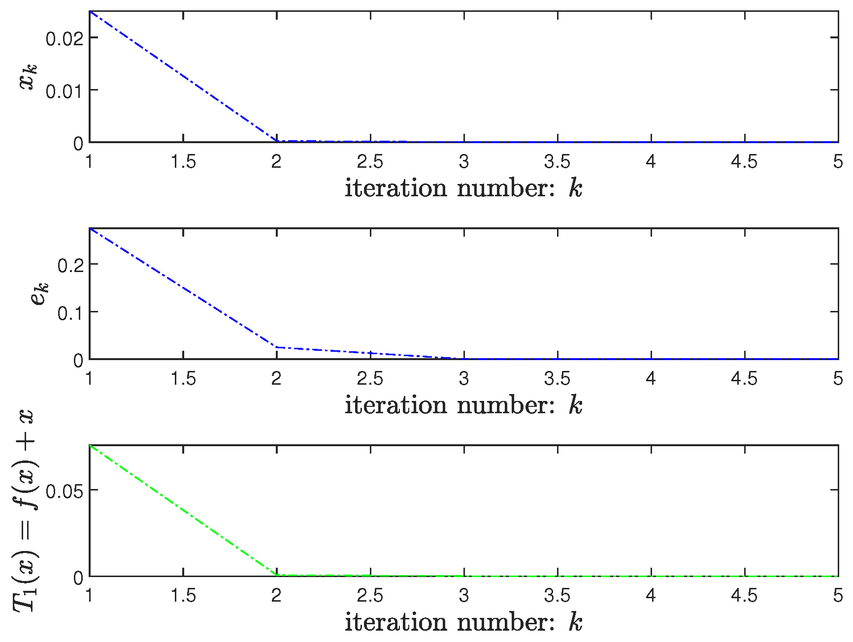
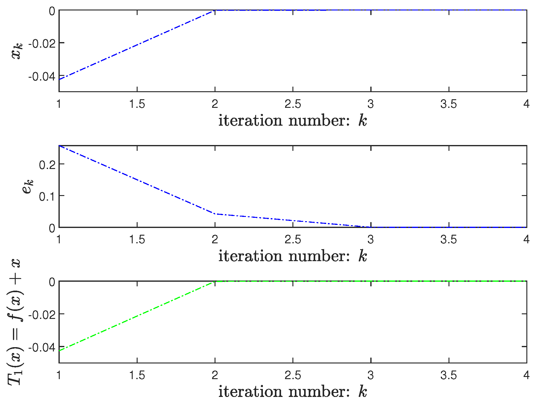
Example 1.

Let $f:\mathbb{R}\to \mathbb{R}$ be such that $f\left(x\right)=x^2+2x$ for all $x\ge 0$, and $f\left(x\right)=x^3$ for all $x<0$. Then, f is not differentiable at 0. Let $n=2,\alpha =0$, and $A:\mathbb{R}\times \mathbb{R}\to \mathbb{R}$ be such that $A(x,u)=(2x+2)u-x^2$ for all $(x,u)\in [0,+\infty )\times \mathbb{R}$ and $A(x,u)=3x^{2}u-2x^3$ for all $(x,u)\in (-\infty ,0)\times \mathbb{R}$. It is clear that A is a $(2,0)$-WPBA at 0 for f. Let $\overline{x}=0,C=[-1,1],\tilde{\theta }=0$, $R_k\equiv 0$ (for all $k\in \mathbb{N}$), and $F:\mathbb{R}\rightrightarrows \mathbb{R}$ be such that $F\left(x\right)=[x,+\infty )$ for all $x\in \mathbb{R}$. It is easy to see that $L_{\overline{x}}$ is metrically regular at 0 for 0, and it is not strongly metrically regular at 0 for 0. Then, it follows from Theorem 1 that, for any $x_0\in [-\frac{1}{6},\frac{1}{6}]$, there exists a sequence $\left\{x_k\right\}$ generated by the proposed method and contained in C which converges to 0 superlinearly of order 2. For each $k\in \mathbb{N}$, let $x_k$ be the kth generation of the proposed method. In fact, if $x_k>0$, we know that any element taken from $[-1,\frac{x_k^2}{2x_k+3}]$ satisfies (8), so we choose $u_k=\frac{x_k^2}{2x_k+3}$. For the case of $x_k<0$, since any element taken from $[-1,\frac{2x_k^3}{3x_k^2+1}]$ satisfies (8), we pick $u_k=\frac{2x_k^3}{3x_k^2+1}$. Note that $u_k\in C$, so we set $x_{k+1}=u_k$. We also have $|x_{k+1}-0|\le \frac{1}{3}{|x_k-0|}^2$. This shows that the sequence $\left\{x_k\right\}$ converges to 0 superlinearly of order 2.

On the other hand, for the starting point $x_0=-\frac{1}{6}\in C$, we can find a sequence $\{-\frac{1}{6},-1,-\frac{1}{6},-1,\dots \}$ which is generated with the proposed method and does not converge to a solution of the aforementioned constrained generalized equation.

Clearly, the condition of $(x_k,u_k)$ satisfying (8) is equivalent to the fact that $u_k\in L_{x_k}^{-1}\left(R_k\left(x_k\right)\right)$. It is easy to observe from Example 1 that $u_k$ should be chosen around the boundary of $L_{x_k}^{-1}\left(R_k\left(x_k\right)\right)$ and not be too far away from the given solution point.

To overcome the shortcoming that not every sequence produced by the general inexact projection method reaches a solution, we examine a modified version of the proposed method for solving nonsmooth constrained generalized equations (Algorithm 2).

Algorithm 2 Restricted generalized inexact projection method

Step 0. Let $x_0\in C$, $\lambda >1$, and $\left\{{\theta }_j\right\}\subset [0,+\infty )$ be given, and set $k=0$. Step 1. If $f\left(x_k\right)+F\left(x_k\right)\ni 0$, then stop; otherwise, compute $u_k\in {\mathbb{R}}^n$ such that $$(A(x_k,u_k)+F\left(u_k\right))\cap R_k\left(x_k\right)\ne \varnothing \mathrm{with}\parallel u_k-\overline{x}\parallel \le \lambda d(\overline{x},L_{x_k}^{-1}\left(R_k\left(x_k\right)\right)).$$ (30) Step 2. If $u_k\in C$, set $x_{k+1}=u_k$; otherwise, take any $x_{k+1}$ satisfying $$x_{k+1}\in P_C(u_k,x_k,{\theta }_k).$$ (31) Step 3. Set $k\leftarrow k+1$, and go to Step 1.

It is clear that (30) is equivalent to the relationship

$$x_{k+1}\in L_{x_k}^{-1}\left(R_k\left(x_k\right)\right)\mathrm{with}\parallel x_{k+1}-\overline{x}\parallel \le \lambda d(\overline{x},L_{x_k}^{-1}\left(R_k\left(x_k\right)\right)).$$

(32)

Since $\lambda >1$, then the restricted generalized inexact projection method is surely executable when $L_x^{-1}\left(R_k\left(x\right)\right)\ne \varnothing$ for any x near $\overline{x}$ and $k\in \mathbb{N}$.

For convergence analysis of the restricted method, we need the following lemma.

Lemma 7.

Assume that the assumptions of Lemmas 3 and 4 hold. Then, for any $x\in B_{r_{*}}\left(\overline{x}\right)$ and $v\in \eta r_{*}^{n+\alpha }{B}_{{\mathbb{R}}^m}$, we have $L_x^{-1}\left(v\right)\ne \varnothing$ and

$$d(\overline{x},L_x^{-1}\left(v\right))\le \frac{\tau }{1-\tau \gamma \left(\kappa \right)\parallel x-\overline{x}{\parallel }^{\alpha }}d(v,L_x\left(\overline{x}\right)).$$

(33)

Proof. 

Pick any $x\in B_{r_{*}}\left(\overline{x}\right)$ and $v\in \eta r_{*}^{n+\alpha }{B}_{{\mathbb{R}}^m}$. Note that $0\in L_{\overline{x}}\left(\overline{x}\right)$. One has

$$A(x,\overline{x})-f\left(\overline{x}\right)\in L_x\left(\overline{x}\right),$$

and then, it follows from (13) that

$$\begin{array}{cc}\hfill d(v,L_x\left(\overline{x}\right))& \le \parallel v+f\left(\overline{x}\right)-A(x,\overline{x})\parallel \hfill \\ & =\parallel v\parallel +\frac{\kappa }{{\pi }_{n,\alpha }}{\parallel x-\overline{x}\parallel }^{n+\alpha }\le \frac{(\kappa +\eta {\pi }_{n,\alpha })r_{*}^{n+\alpha }}{{\pi }_{n,\alpha }}.\hfill \end{array}$$

For any sufficiently small $\epsilon \in \left(0,\frac{1-\tau \gamma \left(\kappa \right)r_{*}^{\alpha }}{\tau }\left(r_{*}-\frac{(\kappa +\eta {\pi }_{n,\alpha })\tau r_{*}^{n+\alpha }}{{\pi }_{n,\alpha }(1-\tau \gamma \left(\kappa \right)r_{*}^{\alpha })}\right)\right)$, take $y\in L_x\left(\overline{x}\right)$ such that $\parallel v-y\parallel <d(v,L_x\left(\overline{x}\right))+\epsilon$. Let

$$\rho :=\frac{\tau \parallel v-y\parallel }{1-\tau \gamma \left(\kappa \right)\parallel x-\overline{x}{\parallel }^{\alpha }}.$$

It is clear that $\rho \le \frac{\tau }{1-\tau \gamma \left(\kappa \right)r_{*}^{\alpha }}\left(\frac{(\kappa +\eta {\pi }_{n,\alpha })r_{*}^{n+\alpha }}{{\pi }_{n,\alpha }}+\epsilon \right)<r_{*}\le a$, and then $B_{\rho }\left(\overline{x}\right)\subset B_{r_{*}}\left(\overline{x}\right)$.

According to the assumption that $L_{\overline{x}}$ is metrically regular at $\overline{x}$ for 0 with constants $\tau ,a$, and b, we conclude that (18) holds, and then $L_{\overline{x}}^{-1}\left(y\right)\ne \varnothing$ for any $y\in B_b\left(0\right)$. By (20), we have $g_x\left(u\right)+v\in B_b\left(0\right)$, and, therefore, ${\mathsf{\Phi }}_{x,v}$ is well defined on $B_{r_{*}}\left(\overline{x}\right)$, where ${\mathsf{\Phi }}_{x,v}$ is defined by (14). Note that $y\in L_x\left(\overline{x}\right)$. We have

$$y+f\left(\overline{x}\right)-A(x,\overline{x})\in L_{\overline{x}}\left(\overline{x}\right).$$

In combination with (18), we have

$$\begin{array}{cc}\hfill d(\overline{x},{\Phi }_{x,v}\left(\overline{x}\right))& =d(\overline{x},L_{\overline{x}}^{-1}(g_x\left(\overline{x}\right)+v)\hfill \\ & \le \kappa d(g_x\left(\overline{x}\right)+v,L_{\overline{x}}\left(\overline{x}\right))\hfill \\ & \le \tau \parallel g_x\left(\overline{x}\right)+v-y-f\left(\overline{x}\right)+A(x,\overline{x})\parallel \hfill \\ & =\tau \parallel v-y\parallel =\rho (1-\tau \gamma \left(\kappa \right)\parallel x-\overline{x}{\parallel }^{\alpha }).\hfill \end{array}$$

Furthermore, for any $u^{\prime },u\in B_{\rho }\left(\overline{x}\right)$, it follows from (22) that

$$e({\mathsf{\Phi }}_x\left(u^{\prime }\right)\cap B_{\rho }\left(\overline{x}\right),{\mathsf{\Phi }}_x\left(u\right))\le \tau \gamma \left(\kappa \right)\parallel x-\overline{x}{\parallel }^{\alpha }\parallel u^{\prime }-u\parallel .$$

Since $\tau \gamma \left(\kappa \right)\parallel x-\overline{x}{\parallel }^{\alpha }<1$, and $B_{\rho }\left(\overline{x}\right)\subset B_{r_{*}}\left(\overline{x}\right)$, by applying Lemma 2 with $\mathsf{\Phi }={\mathsf{\Phi }}_{x,v}$, $\overline{x}=\overline{x},r=\rho$, and $\alpha =\tau \gamma \left(\kappa \right)\parallel x-\overline{x}{\parallel }^{\alpha }$, we obtain a fixed point $u\in {\mathsf{\Phi }}_{x,v}\left(u\right)\cap B_{\rho }\left(\overline{x}\right)$, which establishes that $u\in L_x^{-1}\left(v\right)$ and $\parallel u-\overline{x}\parallel \le \rho$. Then, we have

$$\begin{array}{cc}\hfill d(\overline{x},L_x^{-1}\left(v\right))& \le \rho \le \frac{\tau \parallel v-y\parallel }{1-\tau \gamma \left(\kappa \right)\parallel x-\overline{x}{\parallel }^{\alpha }}\hfill \\ & \le \frac{\tau }{1-\tau \gamma \left(\kappa \right)\parallel x-\overline{x}{\parallel }^{\alpha }}(d(v,L_x\left(\overline{x}\right))+\epsilon ).\hfill \end{array}$$

Since $\epsilon$ is arbitarily chosen, we conclude that (33) holds. □

The following result shows that under proper conditions, every sequence generated with the aforementioned restricted method converges a solution of the nonsmooth constrained generalized equation.

Theorem 2.

Consider the constrained generalized Equation (5) and assume that the assumptions of Theorem 1 hold. Let $\lambda >1$ be such that

$$\frac{\left(1+\sqrt{2\tilde{\theta }}\right)\left(\kappa +\eta {\pi }_{n,\alpha }\right)\lambda \tau r_{*}^{n+\alpha -1}}{{\pi }_{n,\alpha }(1-\tau \gamma \left(\kappa \right)r_{*}^{\alpha })}+\sqrt{2\tilde{\theta }}<1.$$

(34)

Then, for every sequence $\left\{x_k\right\}$ generated by the restricted generalized inexact projection method, which starts from $x_0\in C\cap B_{r_{*}}\left(\overline{x}\right)\setminus \left\{\overline{x}\right\}$, associated with $\left\{{\theta }_k\right\},\left\{R_k\right\}$, and contained in $C\cap B_{r_{*}}\left(\overline{x}\right)$, we have the following convergence:

$$\parallel x_{k+1}-\overline{x}\parallel \le \left[\frac{\left(1+\sqrt{2{\theta }_k}\right)\left(\kappa +\eta {\pi }_{n,\alpha }\right)\lambda \tau {\parallel x_k-\overline{x}\parallel }^{n+\alpha -1}}{{\pi }_{n,\alpha }\left(1-\tau \gamma \left(\kappa \right)\parallel x_k-\overline{x}{\parallel }^{\alpha }\right)}+\sqrt{2{\theta }_k}\right]\parallel x_k-\overline{x}\parallel ,\forall k\in \mathbb{N}.$$

(35)

In particular, if ${\theta }_k=0$ for all $k=0,1,2,\dots$, then

$$\parallel x_{k+1}-\overline{x}\parallel \le \frac{\left(\kappa +\eta {\pi }_{n,\alpha }\right)\lambda \tau }{{\pi }_{n,\alpha }\left(1-\tau \gamma \left(\kappa \right)r_{*}^{\alpha }\right)}{\parallel x_k-\overline{x}\parallel }^{n+\alpha },\forall k\in \mathbb{N}$$

(36)

and $\left\{x_k\right\}$ converges to $\overline{x}$ superlinearly of order $n+\alpha$.

Proof. 

Take any $x,u\in B_{r_{*}}\left(\overline{x}\right)$, and $k\in \mathbb{N}$. By (26), one has $R_k\left(u\right)\subset \eta r_{*}^{n+\alpha }{B}_{{\mathbb{R}}^m}$. Then, it follows from Lemma 7 that $L_x^{-1}\left(R_k\left(u\right)\right)\ne \varnothing$. Since $\lambda >1$, then the restricted generalized inexact projection method is surely executable. Now, pick any $x_0\in C\cap B_{r_{*}}\left(\overline{x}\right)\setminus \left\{\overline{x}\right\}$ and consider any iterative sequence $\left\{x_k\right\}$ generated by the aforementioned method associated with $\left\{{\theta }_k\right\},\left\{R_k\right\}$ and starting at $x_0$. Then, for each $k\in \mathbb{N}$, there exist $u_k$ and $v_k$ associated with $\left\{x_k\right\}$ satisfying

$$v_k\in (A(x_k,u_k)+F\left(u_k\right))\cap R_k\left(x_k\right)\mathrm{and}\parallel u_k-\overline{x}\parallel \le \lambda d(\overline{x},L_{x_k}^{-1}\left(R_k\left(x_k\right)\right)).$$

(37)

If $u_k\in C$, then $x_{k+1}=u_k$; otherwise, $x_{k+1}\in P_C(u_k,x_k,{\theta }_k)$. By (37), one has

$$v_k\in R_k\left(x_k\right),u_k\in L_{x_k}^{-1}\left(v_k\right)\mathrm{and}\parallel u_k-\overline{x}\parallel \le \lambda d(\overline{x},L_{x_k}^{-1}\left(v_k\right)).$$

(38)

Next, we show by induction that $x_k\in B_{r_{*}}\left(\overline{x}\right)$ and (35) holds for each $k\in \mathbb{N}$. Since $0\in L_{\overline{x}}\left(\overline{x}\right)$, we have

$$A(x_0,\overline{x})-f\left(\overline{x}\right)\in L_{x_0}\left(\overline{x}\right).$$

If $u_0\in C$, it follows from (26), (33), and (38) that

$$\begin{array}{cc}\hfill \parallel u_0-\overline{x}\parallel & \le \lambda d(\overline{x},L_{x_0}^{-1}\left(v_0\right))\hfill \\ & \le \frac{\lambda \tau }{1-\tau \gamma \left(\kappa \right)\parallel x_0-\overline{x}{\parallel }^{\alpha }}d(v_0,L_{x_0}\left(\overline{x}\right))\hfill \\ & \le \frac{\lambda \tau }{1-\tau \gamma \left(\kappa \right)\parallel x_0-\overline{x}{\parallel }^{\alpha }}\parallel v_0+f\left(\overline{x}\right)-A(x_0,\overline{x})\parallel \hfill \\ & \le \frac{(\kappa +\eta {\pi }_{n,\alpha })\lambda \tau }{{\pi }_{n,\alpha }(1-\tau \gamma \left(\kappa \right)\parallel x_0-\overline{x}{\parallel }^{\alpha })}{\parallel x_0-\overline{x}\parallel }^{n+\alpha }.\hfill \end{array}$$

(39)

In this case, $x_1=u_0\in C$. Hence, (39) implies that (35) holds for $k=0$. If $u_0\notin C$, then $x_1\in P_C(u_0,x_0,{\theta }_0)\subset C$. Similar to the proof of Lemma 6 when applying (39) in place of (16), we obtain that (35) holds for $k=0$. Note that $x_0\in B_{r_{*}}\left(\overline{x}\right)$. By (34) and (35), one has $\parallel x_1-\overline{x}\parallel \le \parallel x_0-\overline{x}\parallel \le r_{*}$. Hence, $x_1\in C\cap B_{r_{*}}\left(\overline{x}\right)$. Assume for induction that $x_k\in C\cap B_{r_{*}}\left(\overline{x}\right)$ and (35) holds for $k=0,\cdots ,i-1$. Note that $0\in L_{\overline{x}}\left(\overline{x}\right)$. One has

$$A(x_i,\overline{x})-f\left(\overline{x}\right)\in L_{x_i}\left(\overline{x}\right).$$

If $u_i\in C$, it follows from (26), (33), and (38) that

$$\begin{array}{cc}\hfill \parallel u_i-\overline{x}\parallel & \le \lambda d(\overline{x},L_{x_i}^{-1}\left(v_i\right))\hfill \\ & \le \frac{\lambda \tau }{1-\tau \gamma \left(\kappa \right)\parallel x_i-\overline{x}{\parallel }^{\alpha }}d(v_i,L_{x_i}\left(\overline{x}\right))\hfill \\ & \le \frac{\lambda \tau }{1-\tau \gamma \left(\kappa \right)\parallel x_i-\overline{x}{\parallel }^{\alpha }}\parallel v_i+f\left(\overline{x}\right)-A(x_i,\overline{x})\parallel \hfill \\ & \le \frac{(\kappa +\eta {\pi }_{n,\alpha })\lambda \tau }{{\pi }_{n,\alpha }(1-\tau \gamma \left(\kappa \right)\parallel x_i-\overline{x}{\parallel }^{\alpha })}{\parallel x_i-\overline{x}\parallel }^{n+\alpha }.\hfill \end{array}$$

(40)

In this case $x_{i+1}=u_i\in C$, and, hence, (39) implies that (35) holds for $k=i$. If $u_i\notin C$, then $x_{i+1}\in P_C(u_i,x_i,{\theta }_i)$. Similar to the proof of Lemma 6 with the application of (40) instead of (16), we obtain that (35) holds for $k=i$. Note that $x_i\in B_{r_{*}}\left(\overline{x}\right)$. By (34) and (35), one has $\parallel x_{i+1}-\overline{x}\parallel \le \parallel x_i-\overline{x}\parallel \le r_{*}$, and then $x_{i+1}\in C\cap B_{r_{*}}\left(\overline{x}\right)$. Thus, the induction step is complete. Therefore, we have that (35) holds. If ${\theta }_k=0$ for all $k\in \mathbb{N}$, then (36) follows directly from (35). □

4. Numerical Example

In this section, we provide a one-dimensional numerical example to illustrate the pratical performance of our proposed approach.

Example 2.

Consider a nonsmooth constrained generalized equation of the form (5), where $f:\mathbb{R}\to \mathbb{R}$ is defined such that $f\left(x\right)=x^2+2x$ for all $x\ge 0$ and $f\left(x\right)=x^3$ for all $x<0$, $F:\mathbb{R}\rightrightarrows \mathbb{R}$ is defined as $F\left(x\right)=\{x,-x\}$ for all $x\in \mathbb{R}$ and $C=[-1,1]$. It is clear that f is not differentiable at 0. To apply the general inexact projection method, we calculate that $A(x,u)=(2x+2)u-x^2$ for all $(x,u)\in [0,+\infty )\times \mathbb{R}$ and $A(x,u)=3x^{2}u-2x^3$ for all $(x,u)\in (-\infty ,0)\times \mathbb{R}$. It is clear that A is a $(2,0)$-WPBA at 0 for f. Let $\overline{x}=0,\tilde{\theta }=0$, $R_k\equiv 0$ (for all $k\in \mathbb{N}$), and it is easy to see that $L_{\overline{x}}$ is metrically regular at 0 for 0. Recall that the generalized equation contains two branches: $T_1\left(x\right)=f\left(x\right)+x$ and $T_2\left(x\right)=f\left(x\right)-x$. We examine below the performance of the proposed method for $T_1$ and $T_2$, respectively, by choosing $u_k$ according to (8).

In Figure 1 and Figure 2, we consider positive and negative initial points, respectively, and show the values of $x_k$, $T_1\left(x_k\right)$, the distances $e_k=\parallel x_{k+1}-x_k\parallel$, and their relationships with the number of iterations. In Figure 3 and Figure 4, we show the values of $x_k$, $T_2\left(x_k\right)$, the distances $e_k=\parallel x_{k+1}-x_k\parallel$, and their relationships with the number of iterations for both positive and negative initial points. The stop condition is $\parallel x_k-x_{k-1}\parallel \le {10}^{-8}$ or the maximum number of iterations is 50.

Figure 1. $T_1\left(x\right)$ with initial point $x_0=0.3$.

Figure 2. $T_1\left(x\right)$ with initial point $x_0=-0.3$.

Figure 3. $T_2\left(x\right)$ with initial point $x_0=0.4$.

Figure 4. $T_2\left(x\right)$ with initial point $x_0=-0.4$.

5. Conclusions

In this paper, we propose an abstract general iterative procedure for solving nonsmooth constrained generalized equations in which the nonsmooth single-valued mapping admits weak point-based approximations (WPBAs). The proposed method incorporates the aforementioned nonsmoothness property as well as an inexact feasible projection onto the constraint set. We prove higher order convergence of the iterative sequence and establish a relationship between the order of convergence and the parameters of WPBA property. The proposed general inexact projetion method is an extention of the Newton-InexP method which deals with smooth constrained generalized equations to nonsmooth cases. The obtained results are improvements of existing ones in the literature even for cases when the single-valued mapping is smooth or the constraint set vanishes.