Time-Inhomogeneous Finite Birth Processes with Applications in Epidemic Models

Abstract

We consider the evolution of a finite population constituted by susceptible and infectious individuals and compare several time-inhomogeneous deterministic models with their stochastic counterpart based on finite birth processes. For these processes, we determine the explicit expressions of the transition probabilities and of the first-passage time densities. For time-homogeneous finite birth processes, the behavior of the mean and the variance of the first-passage time density is also analyzed. Moreover, the approximate duration until the entire population is infected is obtained for a large population size.

1. Introduction

We consider a “closed” population of a total constant size N. This population is divided into two qualitatively distinct regions $R_1$ and $R_2$, types or compartments, and we assume that only one-way migration from $R_1$ to $R_2$ can occur and that, at time $t=t_0$, there are $N-j$ individuals in $R_1$ and j individuals in $R_2$. We denote by $M\left(t\right)$ the number of individuals in the region $R_2$ at time $t\ge t_0$, with $M\left(t\right)\in \{j,j+1,\dots ,N\}$, so that $M\left(t\right)-j$ individuals at time $t\ge t_0$ have migrated from $R_1$ to $R_2$. The growth of the population in $R_2$ can be described using a finite birth process, the birth of an individual in the region $R_2$ being due to the migration of an individual from $R_1$. The average time required for all individuals to migrate from $R_1$ to the region $R_2$ is a significative parameter to analyze. The stochastic processes that describe the evolution of a population in which the individuals can only be born are discussed, for instance, in Bailey [1], Bharucha-Reid [2], Cox and Miller [3], and Taylor and Karlin [4].

In epidemiology, compartment models are known as “epidemic models” and are often applied to the mathematical modeling of infectious diseases (cf. Allen [5,6], Dailey and Gani [7]). The simplest compartment models assume an individual can be in one of only two states, either susceptible (S) or infectious (I). For $t\ge t_0$, we denote by $S\left(t\right)$ the number of susceptible individuals, by $I\left(t\right)$ the number of individuals infected, and by N the total population size, where $N=S\left(t\right)+I\left(t\right)$ is constant. It is assumed that there are no removals of, no immunities to, and no recoveries from infection. The susceptible individuals become infected through contact with infectious individuals.

A compartmental model with two states can be described with ordinary differential equations in the deterministic dynamics and via finite birth processes in the stochastic approach, which is more realistic but more complicated to analyze. Such models try to predict how a disease spreads, the total number infected, the duration of an epidemic and allow for estimating the various epidemiological parameters. Not all diseases are accurately described by a model with only two states, but a two-state model is useful in describing some classes of micro-parasitic infections to which individuals never acquire a long-lasting immunity and, over the course of the epidemic, everyone eventually becomes infected. An example of a two-state epidemic model is the herpes simplex virus (HSV). Since HSV is a viral infection, it is transmitted via skin to skin contact with infected areas. This form of disease is difficult to control because many individuals who are infected unknowingly spread the disease. The antivirals can help reduce the severity and frequency between breakouts, but there is no cure, so the infected population continues to grow indefinitely. Another example of such a disease is the Cytomegalovirus (CMV), that has the ability to remain latent within the human host.

In Figure 1, a schematic compartmental representation with two states is given.

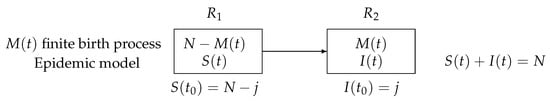
Figure 1. A schematic compartmental representation with two states: susceptible and infectious.

Discrepancies are often observed between the real data and theoretical predictions due to more or less intense environmental fluctuations. One way to overcome this problem is to consider a stochastic approach to the phenomenon. Both deterministic and stochastic models can be used to capture the dynamic of infection in the population and are alternate viewpoints on the same phenomenon, offering complementary insights. The predictions in the deterministic models are determined entirely by their initial conditions, the set of underlying differential equations, and the input intensity functions. The model, based on a system of ordinary differential equations, can be thought of as a deterministic skeleton of any corresponding stochastic model. Starting with a family of ordinary differential equations, which describes a dynamical system, one can arrive at a variety of corresponding stochastic models by interpreting some or all the deterministic rates as stochastic rates. The approach based on continuous-time Markov chains is preferable to the one based on stochastic differential equations, because the former preserves the discrete values of the population. In our study, the number of infected individuals in the population is described using a finite birth process $M\left(t\right)$ (see, for instance, Bailey [1,8], Cox and Miller [3], and Taylor and Karlin [4]). Recent developments in mathematical modeling, with applications in the transmission of infection in population dynamics, are investigated and analyzed in studies by Anggriani et al. [9], Joseph et al. [10], and Jose et al. [11,12].

In two-state stochastic epidemic models, the main purpose of the study is to determine the probability distribution of the number of infected individuals as a function of time, to determine the expected duration until the infected population size reaches N, and to obtain some asymptotic approximations for large N.

Plan of the Paper

In Section 2, we revisit a variety of time-inhomogeneous (TNH) deterministic epidemic models with two states, either susceptible (S) or infectious (I). We study the growth of the infected population and we determine the deterministic time $T^{*}$ required until $N-1$ individuals of the population are infected. In Section 3, we consider the TNH finite birth process $\{M\left(t\right),t\ge t_0\}$ with birth intensity functions ${\lambda }_n\left(t\right)=\lambda \left(t\right)(N-n){\xi }_n$ for $n=j,j+1,\dots ,N$ and we determine the transition probabilities $p_{j,n}\left(t\right|t_0)$ for $M\left(t\right)$ when the birth intensity functions are all distinct, and in the case in which they are not necessarily distinct. The general expression of the first-passage time (FPT) probability density function (pdf) $g_{j,k}\left(t\right|t_0)$ is obtained for $k=j+1,j+2,\dots ,N$. Moreover, the FPT mean and the FPT variance are explicitly evaluated for the time-homogenous (TH) birth process. In Section 4, we take into account the flexible finite birth process in which ${\xi }_n=[{\gamma }_{1}n+{\gamma }_2(N-n)]/N$. For this process, we determine the partial differential equations for the probability generating function (PGF) and for the cumulant generating function (CGF). Moreover, the asymptotic behavior of the mean size of the population is analyzed for large N. Special attention is dedicated to the FPT densities and to the FPT moments for the TNH-binomial birth process $({\gamma }_1={\gamma }_2=1)$, TNH-quadratic birth process $({\gamma }_1=0,{\gamma }_2=1)$, and TNH-SI birth process $({\gamma }_1=1,{\gamma }_2=0)$. In Section 5, we consider the stochastic hyper-logistic birth process in which ${\xi }_n={(N-n)}^p{n}^{1-p}/N$, with $0<p<1$. The FPT pdf and the FPT moments are studied for different choices of the parameter $p\in (0,1)$. For the TH-binomial, TH-quadratic, TH-SI, and TH-hyper-logistic birth processes, the numerical results show that the deterministic time required until $N-1$ individuals of the population are infected is always included in the interval $\left(\mathrm{E}\left[{\mathcal{T}}_{j,N-1}\right],\mathrm{E}\left[{\mathcal{T}}_{j,N}\right]\right)$, where $\mathrm{E}\left[{\mathcal{T}}_{j,k}\right]$ denotes the average of the FPT from j to k. Various numerical computations are performed with MATHEMATICA to analyze the role played by the parameters.

2. Deterministic Epidemic Models with Two States

We consider some deterministic epidemic models with two states, either susceptible (S) or infectious (I).

2.1. Flexible Birth Model

The following is a flexible two-state epidemic model:

$$\begin{array}{cc}\hfill & \frac{dS\left(t\right)}{dt}=-\frac{\lambda \left(t\right)}{N}S\left(t\right)\left[{\gamma }_{1}I\left(t\right)+{\gamma }_{2}S\left(t\right)\right],\hfill \\ \hfill & \frac{dI\left(t\right)}{dt}=\frac{\lambda \left(t\right)}{N}S\left(t\right)\left[{\gamma }_{1}I\left(t\right)+{\gamma }_{2}S\left(t\right)\right],\hfill \end{array}$$

(1)

with $S\left(t\right)+I\left(t\right)=N$ for $t\ge t_0$, where ${\gamma }_1\ge 0$, ${\gamma }_2\ge 0$, ${\gamma }_1+{\gamma }_2>0$ and the transmission intensity function $\lambda \left(t\right)$ is a positive, bounded, and continuous function of t. The replacement of $S\left(t\right)=N-I\left(t\right)$ into (1) leads to the flexible growth curve for $I\left(t\right)$, described with the following differential equation:

$$\frac{dI\left(t\right)}{dt}=\frac{\lambda \left(t\right)}{N}\left[N-I\left(t\right)\right]\left\{{\gamma }_{1}I\left(t\right)+{\gamma }_2[N-I\left(t\right)]\right\},t>t_0,$$

(2)

whose solution for $t\ge t_0$ is as follows:

$$I\left(t\right)=\left\{\begin{array}{cc}{\displaystyle \frac{N\left\{I\left(t_0\right)+{\gamma }_2[N-I\left(t_0\right)]\Lambda \left(t\right|t_0)\right\}}{N+{\gamma }_2[N-I\left(t_0\right)]\Lambda \left(t\right|t_0)},}\hfill & {\gamma }_1=0,\hfill \\ {\displaystyle \frac{N\left\{{\gamma }_{1}I\left(t_0\right)+{\gamma }_2[N-I\left(t_0\right)]\left(1-e^{-{\gamma }_1\Lambda \left(t\right|t_0}\right)\right\}}{{\gamma }_{1}I\left(t_0\right)+[N-I\left(t_0\right)]\left[{\gamma }_1{e}^{-{\gamma }_1\Lambda \left(t\right|t_0)}+{\gamma }_2\left(1-e^{-{\gamma }_1\Lambda \left(t\right|t_0}\right)\right]},}\hfill & {\gamma }_1>0,\hfill \end{array}\right.$$

(3)

where

$$\Lambda \left(t\right|t_0)={\int }_{t_0}^t\lambda \left(\theta \right)d\theta .$$

(4)

Indeed, by making the change of variable $Z\left(t\right)=[N-I(t\left)\right]/I\left(t\right)$ in (2), one obtains the differential equation $dZ\left(t\right)/dt=-\lambda \left(t\right)Z\left(t\right)\left[{\gamma }_1+{\gamma }_{2}Z\left(t\right)\right]$; by solving this last equation and recalling the performed change of variable, one is led to (3). Since ${\gamma }_1\ge 0$, ${\gamma }_2\ge 0$ with ${\gamma }_1+{\gamma }_2>0$, $I\left(t\right)$ is an increasing function of t, if ${lim}_{t\to +\infty }\Lambda \left(t\right|t_0)=+\infty$, at the end, every individual of the population becomes infected, i.e., ${lim}_{t\to +\infty }I\left(t\right)=N$. Moreover, if $\lambda \left(t\right)=\lambda$ for all t, one has the following:

• If ${\gamma }_2\ge {\gamma }_1/2$, no inflection point exists;
• If $0\le {\gamma }_2<{\gamma }_1/2$, a unique inflection point in (3) exists that occurs at the level

  $$L=\frac{N({\gamma }_1-2{\gamma }_2)}{2({\gamma }_1-{\gamma }_2)}$$

  when $I\left(t_0\right)<L<N$, otherwise no inflection point exists.

The time until the infected population size reaches N is infinite, because N is approached asymptotically. To obtain an estimate of the time $T^{*}$ required until $N-1$ individuals of the population are infected, we solve the equation $I\left(T^{*}\right)=N-1$. For the flexible model with $\lambda \left(t\right)=\lambda$, by virtue of (3), one has the following:

$$T^{*}=\left\{\begin{array}{cc}{\displaystyle t_0+\frac{1}{\lambda {\gamma }_2}\frac{N[N-1-I\left(t_0\right)]}{N-I\left(t_0\right)},}\hfill & {\gamma }_1=0,\hfill \\ {\displaystyle t_0+\frac{1}{\lambda {\gamma }_1}ln\left\{\frac{[N-I\left(t_0\right)][(N-1){\gamma }_1+{\gamma }_2]}{{\gamma }_{1}I\left(t_0\right)+{\gamma }_2[N-I\left(t_0\right)]}\right\},}\hfill & {\gamma }_1>0.\hfill \end{array}\right.$$

(5)

We remark that the flexible model includes the Bass model, which is used in marketing and forecasting to describe the diffusion of new products, services, or innovations. The Bass model can be expressed mathematically as follows (cf. Mahajan et al. [13], Guidolin and Manfredi [14]):

$$\frac{dA\left(t\right)}{dt}=\alpha [N-A\left(t\right)]+\frac{\beta }{N}A\left(t\right)[N-A\left(t\right)],t>t_0,$$

(6)

with $\alpha >0$ and $\beta >0$, where $A\left(t\right)$ is the number of adopters at time t, N is the potential market size (the total number of potential adopters), $\alpha$ is the coefficient of innovation (the rate at which early adopters adopt the product), and $\beta$ is the coefficient of imitation (the rate at which late adopters adopt the product). Indeed, by choosing $\lambda \left(t\right)=\lambda$, ${\gamma }_1=(\alpha +\beta )/\lambda$, and ${\gamma }_2=\alpha /\lambda$, Equation (2) identifies with the Bass differential Equation (6).

There are three special cases of the flexible model obtainable by choosing appropriately the parameters ${\gamma }_1$ and ${\gamma }_2$: the binomial model, quadratic model, and SI model.

2.1.1. Binomial Birth Model

For ${\gamma }_1={\gamma }_2=1$ in (1), one obtains the following:

$$\frac{dS\left(t\right)}{dt}=-\lambda \left(t\right)S\left(t\right),\frac{dI\left(t\right)}{dt}=\lambda \left(t\right)S\left(t\right),$$

(7)

with $S\left(t\right)+I\left(t\right)=N$ for $t\ge t_0$. Equation (7) leads to the binomial growth curve for $I\left(t\right)$ described with the differential equation:

$$\frac{dI\left(t\right)}{dt}=\lambda \left(t\right)\left[N-I\left(t\right)\right],t>t_0,$$

the solution of which is as follows:

$$I\left(t\right)=N-[N-I\left(t_0\right)]e^{-\Lambda \left(t\right|t_0)},t\ge t_0.$$

(8)

If $\lambda \left(t\right)=\lambda$ for all t, no inflection point is present in the binomial model.

2.1.2. Quadratic Birth Model

For ${\gamma }_1=0$ and ${\gamma }_2=1$ in (1), one has the following:

$$\frac{dS\left(t\right)}{dt}=-\frac{\lambda \left(t\right)}{N}{S}^2\left(t\right),\frac{dI\left(t\right)}{dt}=\frac{\lambda \left(t\right)}{N}{S}^2\left(t\right),$$

(9)

with $S\left(t\right)+I\left(t\right)=N$ for $t\ge t_0$. Equation (9) leads to the quadratic growth curve for $I\left(t\right)$ described with the following differential equation:

$$\frac{dI\left(t\right)}{dt}=\frac{\lambda \left(t\right)}{N}{\left[N-I\left(t\right)\right]}^2,t>t_0,$$

the solution of which is

$$I\left(t\right)=\frac{N\left\{I\left(t_0\right)+\Lambda \left(t\right|t_0)[N-I\left(t_0\right)]\right\}}{N+\Lambda \left(t\right|t_0)[N-I\left(t_0\right)]},t\ge t_0.$$

(10)

If $\lambda \left(t\right)=\lambda$ for all t, no inflection point is present in the quadratic model (10).

2.1.3. SI Birth Model

For ${\gamma }_1=1$ and ${\gamma }_2=0$ in (1), one obtains the SI model

$$\frac{dS\left(t\right)}{dt}=-\frac{\lambda \left(t\right)}{N}S\left(t\right)I\left(t\right),\frac{dI\left(t\right)}{dt}=\frac{\lambda \left(t\right)}{N}S\left(t\right)I\left(t\right),$$

(11)

with $S\left(t\right)+I\left(t\right)=N$ for $t\ge t_0$. Equation (11) leads to the Verhulst logistic growth curve for $I\left(t\right)$ described with the following differential equation:

$$\frac{dI\left(t\right)}{dt}=\frac{\lambda \left(t\right)}{N}\left[N-I\left(t\right)\right]I\left(t\right),t>t_0,$$

the solution of which is

$$I\left(t\right)=\frac{NI\left(t_0\right)}{I\left(t_0\right)+[N-I\left(t_0\right)]e^{-\Lambda \left(t\right|t_0)}},t\ge t_0.$$

(12)

In the Verhulst logistic model (12), if $\lambda \left(t\right)=\lambda$, the inflection point occurs at the level $L=N/2$ when $L>I\left(t_0\right)$.

In Figure 2, we consider the flexible two-state epidemic model (1) with $\lambda \left(t\right)=0.4[1+0.9cos(2\pi t\left)\right]$; the curves $I\left(t\right)$ and $S\left(t\right)=N-I\left(t\right)$ are plotted as functions of t for $N=200$, $I\left(0\right)=20$, $S\left(0\right)=180$, and for some choices of the parameters ${\gamma }_1$ and ${\gamma }_2$. Figure 2a refers to the SI epidemic model, Figure 2c relates to the binomial epidemic model, and Figure 2d puts emphasis on the quadratic epidemic model.

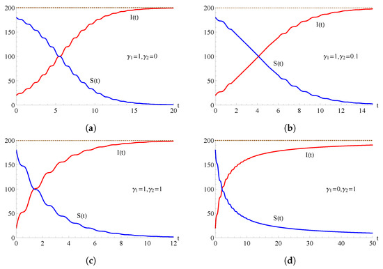
Figure 2. For the flexible model with $\lambda \left(t\right)=0.4[1+0.9cos(2\pi t\left)\right]$, the population of the infected $I\left(t\right)$ (red curve) and of the susceptible $S\left(t\right)$ (blue curve) are plotted as functions of t for $N=200$, $I\left(0\right)=20$, $S\left(0\right)=180$, and for some choices of the parameters ${\gamma }_1$ and ${\gamma }_2$. In (a) ${\gamma }_1=1,{\gamma }_2=0$, in (b) ${\gamma }_1=1,{\gamma }_2=0.1$, in (c) ${\gamma }_1=1,{\gamma }_2=1$ and in (d) ${\gamma }_1=0,{\gamma }_2=1$.

In Table 1, for the binomial, SI, and quadratic models, the duration $T^{*}$ until $N-1$ individuals of a population are infected is indicated for $t_0=0$, $I\left(0\right)=20$, $N=200$, and various choices of $\lambda$. The values of $T^{*}$ in Table 1 are obtained from (5) by setting ${\gamma }_1={\gamma }_2=1$ for the binomial model, ${\gamma }_1=1$, ${\gamma }_2=0$ for the SI model, and ${\gamma }_1=0$, ${\gamma }_2=1$ for the quadratic model.

Table 1. The duration $T^{*}$, given in (5), is indicated for $t_0=0$, $I\left(0\right)=20$, $N=200$, and various choices of $\lambda$.

$\mathit{\lambda }$	Binomial Model	SI Model	Quadratic Model
0.4	12.9824	18.7263	497.222
0.8	6.49120	9.36316	248.611
1.2	4.32746	6.24211	165.741
1.6	3.24560	4.68158	124.306
2.0	2.59648	3.74526	99.4444

2.2. General Finite Birth Models

In two-state epidemic models, it is often realistic to introduce an interaction term of the form $S\left(t\right)\phi \left[I\right(t\left)\right]$, where the dependence on the number of infected individuals occurs via a nonlinear bounded function $\phi \left[I\right(t\left)\right]$ (cf. Dong et al. [15]).

$$\frac{dS\left(t\right)}{dt}=-\lambda \left(t\right)S\left(t\right)\phi \left[I\left(t\right)\right],\frac{dI\left(t\right)}{dt}=\lambda \left(t\right)S\left(t\right)\phi \left[I\left(t\right)\right],$$

(13)

with $S\left(t\right)+I\left(t\right)=N$ for $t\ge t_0$. In particular, if $\phi \left[I\left(t\right)\right]=[{\gamma }_{1}I\left(t\right)+{\gamma }_2[N-I\left(t\right)]/N$, with ${\gamma }_1\ge 0$, ${\gamma }_2\ge 0$, ${\gamma }_1+{\gamma }_2>0$, one obtains the flexible growth curve (3) for $I\left(t\right)$.

Hyper-Logistic Birth Model

If $\phi \left[I\left(t\right)\right]={\left[I\left(t\right)\right]}^{1-p}{[N-I\left(t\right)]}^p/N$ in (13), with $0<p\le 1$, one obtains the hyper-logistic model described by the differential equation for $I\left(t\right)$

$$\frac{dI\left(t\right)}{dt}=\frac{\lambda \left(t\right)}{N}{\left[I\left(t\right)\right]}^{1-p}{\left[N-I\left(t\right)\right]}^{1+p},t>t_0,$$

(14)

whose solution is as follows (cf. Turner et al. [16], Anguelov et al. [17], and Albano et al. [18]):

$$I\left(t\right)=\frac{N}{1+{\left[p\Lambda \left(t\right|t_0)+{\left(\frac{N-I\left(t_0\right)}{I\left(t_0\right)}\right)}^{-p}\right]}^{-1/p}},t\ge t_0.$$

(15)

Indeed, by performing the change of variable $Z\left(t\right)=[N-I(t\left)\right]/I\left(t\right)$ in (14), one has the differential equation $dZ\left(t\right)/dt=-\lambda \left(t\right){\left[Z\left(t\right)\right]}^{p+1}$; by solving this last equation and recalling the considered change of variable, one obtains (15). In particular, when $p\to 0$ the hyper-logistic growth curve (15) converges to the Verhulst logistic growth curve (12), being

$$\underset{p\to 0}{lim}{\left[p\Lambda \left(t\right|t_0)+{\left(\frac{N-I\left(t_0\right)}{I\left(t_0\right)}\right)}^{-p}\right]}^{-1/p}=\frac{N-I\left(t_0\right)}{I\left(t_0\right)}{e}^{-\Lambda \left(t\right|t_0)}.$$

Moreover, when $p=1$, Equation (15) identifies the quadratic growth curve (10).

The hyper-logistic model, defined using Equation (14), helps to overcome the major limitation of the Verhulst logistic model: the inflexibility of the inflection point. Specifically, in the Verhulst logistic model, the inflection point is fixed at $N/2$, whereas, in the hyper-logistic curve (15), with $0<p<1$ and $\lambda \left(t\right)=\lambda$ for all t, the inflection point occurs at the level $L=N(1-p)/2$ when $I\left(t_0\right)<L<N$ and it does not exist otherwise. Moreover, for the hyper-logistic model with $\lambda \left(t\right)=\lambda$, the duration $T^{*}$ until $N-1$ individuals of a population are infected is

$$T^{*}=t_0+\frac{1}{\lambda p}\left\{{(N-1)}^p-{\left(\frac{I\left(t_0\right)}{N-I\left(t_0\right)}\right)}^p\right\},0<p\le 1.$$

(16)

In Figure 3, we consider the hyper-logistic two-state epidemic model with $\lambda \left(t\right)=0.4[1+0.9cos(2\pi t\left)\right]$; the curves $I\left(t\right)$ and $S\left(t\right)=N-I\left(t\right)$ are plotted as functions of t for $N=200$, $I\left(0\right)=20$, $S\left(0\right)=180$, and for some choices of the parameter p.

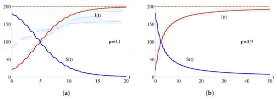
Figure 3. For the hyper-logistic model with $\lambda \left(t\right)=0.4[1+0.9cos(2\pi t\left)\right]$, the population of the infected $I\left(t\right)$ (red curve) and of the susceptible $S\left(t\right)$ (blue curve) are plotted as functions of t for $N=200$, $I\left(0\right)=20$, $S\left(0\right)=180$, and for some choices of the parameter p. In (a) $p=0.1$ and in (b) $p=0.9$.

In Table 2, for the hyper-logistic model, the duration $T^{*}$, given in (16), is indicated for $t_0=0$, $I\left(0\right)=20$, $N=200$, and various choices of $\lambda$ and p.

Table 2. For the hyper-logistic model, the duration $T^{*}$ is listed for $t_0=0$, $I\left(0\right)=20$, $N=200$, and various choices of $\lambda$ and p.

p	$\mathit{\lambda }=0.4$	$\mathit{\lambda }=0.8$	$\mathit{\lambda }=1.2$	$\mathit{\lambda }=1.6$	$\mathit{\lambda }=2.0$
0.1	22.3763	11.1882	7.45878	5.59409	4.47527
0.5	68.8670	34.4335	22.9557	17.2168	13.7734
0.9	325.201	162.601	108.400	81.3003	65.0402

As highlighted in Figure 2 and Figure 3, the intersection of the two curves at the level $N/2$ represents an equilibrium where the numbers of susceptible individuals and infected individuals are equal. After the equilibrium point, the population includes more infected individuals and fewer susceptible individuals. This trend continues until, ultimately, every individual is included in the infectious population so that, ultimately, the whole population becomes infected.

We remark that the hyper-logistic differential Equation (14) is a special case of the Blumberg growth model

$$\frac{dI\left(t\right)}{dt}=\frac{\lambda \left(t\right)}{N^{\alpha +\beta -1}}{\left[I\left(t\right)\right]}^{\alpha }{\left[N-I\left(t\right)\right]}^{\beta },t>t_0,$$

(17)

where $\alpha >0$ and $\beta >1$ are shape parameters. The Blumberg growth model (17) is an extension of the Verhulst logistic growth equation and is used to describe several demographic, economic, ecological, and biological models (cf. Blumberg [19], Rocha and Aleixo [20]). By setting $\alpha =1-p$ and $\beta =1+p$ in (17), we obtain the hyper-logistic growth differential Equation (14).

We note that, in all the deterministic models previously considered, the results are as follows:

• The form of the transmission intensity function $\lambda \left(t\right)$ has a significant impact on the population dynamics of the infected $I\left(t\right)$ and of the susceptible $S\left(t\right)=N-I\left(t\right)$;
• $I\left(t\right)$ is an increasing function of t and $S\left(t\right)$ is a decreasing function of t;
• If ${lim}_{t\to +\infty }\Lambda \left(t\right|t_0)=+\infty$, at the end, all individuals of the population are infected, i.e., ${lim}_{t\to +\infty }I\left(t\right)=N$;
• The time T until the infected population size reaches N, i.e., $I\left(T\right)=N$, is actually infinite because N is approached asymptotically;
• The duration $T^{*}$ until $N-1$ individuals of a population are infected provides a measure of the growth time of the infection in the epidemic model.

3. The Stochastic Finite Birth Process

Let $\{M\left(t\right),t\ge t_0\}$ be a TNH finite birth process having state-space $\{j,j+1,\dots ,N\}$, $0\le j<N$, with birth intensity functions ${\lambda }_n\left(t\right)$, where N denotes the constant total population size (see Figure 4).

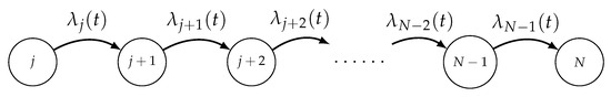
Figure 4. The state diagram of the TNH finite birth process $M\left(t\right)$.

To reach the size n $(j<n\le N)$ from its initial size j, the population goes from j to $j+1$, then from $j+1$ to $j+2$, …, at end from $n-1$ to n, in this precise order.

In epidemiology, the process $M\left(t\right)$ describes the number of infected individuals and $N-M\left(t\right)$ represents the number of susceptible individuals at time t. Once infected, and with no treatment, individuals stay infected and remain in contact with the susceptible population.

For the finite birth process $M\left(t\right)$, we assume that the births at time t occur with intensity functions given by

$${\lambda }_n\left(t\right)=\lambda \left(t\right)(N-n){\xi }_n,n=j,j+1,\dots ,N,$$

(18)

where ${\xi }_n>0$ depends on the state n of the system (number of infected individuals) and where $\lambda \left(t\right)$ is a positive, bounded, and continuous function of t. In Equation (18), the dependence of $\lambda \left(t\right)$ on t defines the type of process. If $\lambda \left(t\right)$ is constant for all t, the process is TH, whereas if $\lambda \left(t\right)$ is a function of t, then the process is TNH. In a study by Faddy and Fenlon [21], stochastic models based on TH finite birth processes of type (18) are constructed to describe the invasion in parasite–host systems and various forms for the birth (invasion) rates are proposed. Marrec et al. [22] describe the population growth as a stochastic birth process and compare the average size of the population with the solution obtained via the deterministic approach.

For $t\ge t_0$, let

$$p_{j,n}\left(t\right|t_0)=P\{M\left(t\right)=n|M\left(t_0\right)=j\},n=j,j+1,\dots ,N,$$

be the transition probabilities of $M\left(t\right)$. They satisfy the Kolmogorov forward equations:

$$\begin{array}{ccc}& & \frac{d{p}_{j,j}\left(t\right|t_0)}{dt}=-(N-j){\xi }_j\lambda \left(t\right)p_{j,j}\left(t\right|t_0),\hfill \\ & & \frac{d{p}_{j,n}\left(t\right|t_0)}{dt}=-(N-n){\xi }_n\lambda \left(t\right)p_{j,n}\left(t\right|t_0)+(N-n+1){\xi }_{n-1}\lambda \left(t\right)p_{j,n-1}\left(t\right|t_0),\hfill \\ & & n=j+1,\dots ,N-1,\hfill \\ & & \frac{d{p}_{j,N}\left(t\right|t_0)}{dt}={\xi }_{N-1}\lambda \left(t\right)p_{j,N-1}\left(t\right|t_0),\hfill \end{array}$$

(19)

with the initial condition ${lim}_{t\downarrow t_0}{p}_{j,n}\left(t\right|t_0)={\delta }_{j,n}$, where ${\delta }_{j,n}$ is the Kronecker delta function. For the TNH finite birth process $M\left(t\right)$, with birth intensity functions (18), one has ${\sum }_{n=j}^N{p}_{j,n}\left(t\right|t_0)=1$. Moreover, from the first equation in (19), one obtains the following:

$$p_{j,j}\left(t\right|t_0)=e^{-(N-j){\xi }_j\Lambda \left(t\right|t_0)},$$

(20)

where $\Lambda \left(t\right|t_0)$ is defined in (4).

To determine the transition probabilities of $M\left(t\right)$, we consider the TH finite birth process $\tilde{M}\left(t\right)$ obtained from $M\left(t\right)$ by setting $\lambda \left(t\right)=1$ in (18) and we denote by ${\tilde{p}}_{j,n}\left(t\right)\equiv {\tilde{p}}_{j,n}\left(t\right|0)$ the transition probabilities of $\tilde{M}\left(t\right)$. From (19), we note that

$$p_{j,n}\left(t\right|t_0)={\tilde{p}}_{j,n}[\Lambda \left(t\right)|\Lambda \left(t_0\right)]={\tilde{p}}_{j,n}[\Lambda \left(t\right|t_0)],n=j,j+1,\dots ,N,$$

(21)

with $\Lambda \left(t\right)\equiv \Lambda \left(t\right|0)$. Therefore, we now focus on the evaluation of the transition probabilities ${\tilde{p}}_{j,n}\left(t\right)$ of $\tilde{M}\left(t\right)$.

We denote by ${\tilde{\Pi }}_{j,n}\left(s\right)$ the Laplace transform (LT) of the transition probability ${\tilde{p}}_{j,n}\left(t\right)$:

$${\tilde{\Pi }}_{j,n}\left(s\right)={\int }_0^{+\infty }{e}^{-st}{\tilde{p}}_{j,n}\left(t\right)dt,s>0.$$

Taking the LT in (19) with $t_0=0$ and $\lambda \left(t\right)=1$, and recalling the initial condition, one has the following:

$$\begin{array}{ccc}& & [s+(N-j){\xi }_j]{\tilde{\Pi }}_{j,j}\left(s\right)=1,\hfill \\ & & [s+(N-n){\xi }_n]{\tilde{\Pi }}_{j,n}\left(s\right)=(N-n+1){\xi }_{n-1}{\tilde{\Pi }}_{j,n-1}\left(s\right),n=j+1,\dots ,N-1,\hfill \\ & & s{\tilde{\Pi }}_{j,N}\left(s\right)={\xi }_{N-1}{\tilde{\Pi }}_{j,N-1}\left(s\right).\hfill \end{array}$$

(22)

Solving Equation (22) using consecutive iterations, one finds the following:

$$\begin{array}{ccc}& & {\tilde{\Pi }}_{j,j}\left(s\right)=\frac{1}{s+(N-j){\xi }_j},\hfill \\ & & {\tilde{\Pi }}_{j,n}\left(s\right)=\frac{(N-n+1)(N-n+2)\cdots (N-j){\xi }_{n-1}{\xi }_{n-2}\cdots {\xi }_j}{[s+(N-n){\xi }_n][s+(N-n+1){\xi }_{n-1}]\cdots [s+(N-j){\xi }_j]},\hfill \\ & & n=j+1,\dots ,N-1,\hfill \\ & & {\tilde{\Pi }}_{j,N}\left(s\right)=\frac{{\xi }_{N-1}}{s}{\tilde{\Pi }}_{j,N-1}\left(s\right).\hfill \end{array}$$

(23)

By taking the inverse LT in the first equation in (23), one has ${\tilde{p}}_{j,j}\left(t\right)=e^{-(N-j){\xi }_{j}t},$ so that, by virtue of (21), one obtains (20). Moreover, for $n=j+1,j+2,\dots ,N$, the determination of the inverse Laplace transforms ${\tilde{p}}_{j,n}\left(t\right)$ of $\tilde{M}\left(t\right)$ via (23) can be obtained by focusing on the sequence of rates ${\xi }_j,{\xi }_{j+1},\dots ,\dots ,{\xi }_N$ and on the multiplicity of the roots of the denominators. Then, via (21), one can derive the required probabilities $p_{j,n}\left(t\right|t_0)$ of $M\left(t\right)$.

Following this approach, we now determine the transition probabilities $p_{j,n}\left(t\right|t_0)$ for the birth process $M\left(t\right)$ under the assumption that the birth intensity functions ${\lambda }_n\left(t\right)$ are all distinct.

Proposition 1.

For the TNH finite birth process $M\left(t\right)$, if the birth intensity functions ${\lambda }_j\left(t\right),$${\lambda }_{j+1}\left(t\right),\dots ,{\lambda }_{N-1}\left(t\right)$, defined in (18), are all distinct, i.e., if

$$(N-i){\xi }_i\ne (N-k){\xi }_{k}i,k=j,j+1,\dots ,N-1,i\ne k,$$

(24)

this results in the following:

$$p_{j,n}\left(t\right|t_0)=\sum _{r=j}^n{A}_{j,n}^{\left(r\right)}{e}^{-(N-r){\xi }_r\Lambda \left(t\right|t_0)},n=j,j+1,\dots ,N,$$

(25)

where, for $r=j,j+1,\dots ,n$ one has the following:

$$A_{j,n}^{\left(r\right)}=\left\{\begin{array}{cc}1,\hfill & n=j\hfill \\ \\ {\displaystyle \frac{(N-j)!}{(N-n)!}\frac{{\xi }_j{\xi }_{j+1}\cdots {\xi }_{n-1}}{{\displaystyle \prod _{\begin{array}{c}i=j\\ i\ne r\end{array}}^n[(N-i){\xi }_i-(N-r){\xi }_r]}},}\hfill & n=j+1,j+2,\dots ,N\hfill \end{array}\right.$$

(26)

and $A_{j,N}^{\left(N\right)}=1$.

Proof. 

Since (24) holds, a partial fraction expansion of the right-hand side of (23) then yields the following:

$${\tilde{\Pi }}_{j,n}\left(s\right)=\sum _{r=j}^n\frac{A_{j,n}^{\left(r\right)}}{s+(N-r){\xi }_r},n=j,j+1,\dots ,N,$$

(27)

where the coefficients

$$A_{j,n}^{\left(r\right)}=\underset{s\to -(N-r){\xi }_r}{lim}[s+(N-r){\xi }_r]{\tilde{\Pi }}_{j,n}\left(s\right).$$

(28)

When $n=j$, by comparing (27) with the first of (23), one has $A_{j,j}^{\left(j\right)}=1$, whereas Equation (26) follows from (23) and (28) for $n=j+1,\dots ,N$. In particular, for $r=n=N$ one has

$$A_{j,N}^{\left(N\right)}=\underset{s\to 0}{lim}s{\tilde{\Pi }}_{j,N}\left(s\right)={\xi }_{N-1}{\tilde{\Pi }}_{j,N-1}\left(0\right)=1.$$

Hence, by taking the inverse Laplace transform of (27), one obtains the following (cf. Erdèlyi et al. [23], p. 232, n. 20):

$${\tilde{p}}_{j,n}\left(t\right)=\sum _{r=j}^n{A}_{j,n}^{\left(r\right)}{e}^{-(N-r){\xi }_{r}t}n=j,j+1,\dots ,N,$$

from which, due to (21), Equation (25) follows. □

From the last equation in (19), by virtue of (21), we obtain the following alternative expression:

$$p_{j,N}\left(t\right|t_0)={\xi }_{N-1}\sum _{r=j}^{N-1}\frac{A_{j,N-1}^{\left(r\right)}}{(N-r){\xi }_r}\left[1-e^{-(N-r){\xi }_r\Lambda \left(t\right|t_0))}\right],0\le j<N.$$

Under the assumptions of Proposition 1, if ${lim}_{t\to +\infty }\Lambda \left(t\right|t_0)=+\infty$ from (25) one has ${lim}_{t\to +\infty }{p}_{j,N}\left(t\right|t_0)=1$ and ${lim}_{t\to +\infty }{p}_{j,n}\left(t\right|t_0)=0$ for $n=j,j+1,\dots ,N-1$.

For a TH finite birth process $\tilde{M}\left(t\right)$, the results of Proposition 1 are in agreement with those given in the study of Bharucha-Reid [2], p. 185, for $j=0$.

We now determine the transition probabilities $p_{j,n}\left(t\right|t_0)$ for the process $M\left(t\right)$ under the assumption that the birth intensity functions ${\lambda }_n\left(t\right)$ are not necessarily distinct. To this aim, for fixed j and n, with $n=j,j+1,\dots ,N$, we consider the sequence of birth rates $(N-j){\xi }_j,(N-j+1){\xi }_{j+1},\dots ,(N-n+1){\xi }_{n-1},(N-n){\xi }_n$ and we denote by ${\alpha }_1(j,n),{\alpha }_2(j,n),\dots ,{\alpha }_d(j,n)$ the distinct values of the sequence and we indicate by $m_1(j,n),$$m_2(j,n),\dots ,$$m_d(j,n)$ their respective multiplicities, with $m_1(j,n)+m_2(j,n)+\dots +m_d(j,n)=n-j+1$ and ${\alpha }_i(j,n)\ge 0$.

Proposition 2.

Let j, n and N be fixed parameters, with $j\le n\le N$. For the TNH finite birth process $M\left(t\right)$, with intensity functions defined in (18), this results in the following:

$$p_{j,n}\left(t\right|t_0)=\sum _{k=1}^d\sum _{\ell =1}^{m_k(j,n)}\frac{B_{j,n}^{(k,\ell )}{[\Lambda \left(t\right|t_0)]}^{m_k(j,n)-\ell }}{[m_k(j,n)-\ell ]!(\ell -1)!}{e}^{-{\alpha }_k(j,n)\Lambda \left(t\right|t_0)},$$

(29)

where for $k=1,2,\dots ,d$ and $\ell =1,2,\dots ,m_k(j,n)$ one has the following:

$$B_{j,n}^{(k,\ell )}=\frac{(N-j)!}{(N-n)!}{\xi }_j{\xi }_{j+1}\cdots {\xi }_{n-1}\underset{s\to -{\alpha }_k(j,n)}{lim}\frac{d^{\ell -1}}{d{s}^{\ell -1}}\frac{{\left[s+{\alpha }_k(j,n)\right]}^{m_k(j,n)}}{{\prod }_{i=1}^d{\left[s+{\alpha }_i(j,n)\right]}^{m_i(j,n)}}·$$

(30)

Proof. 

We suppose that j, n, and N are fixed parameters, with $j\le n\le N$. To determine the inverse LT of ${\tilde{\Pi }}_{j,n}\left(s\right)$, given in (23), we consider the polynomial of degree $n-j+1$ in s

$$Q_{j,n}\left(s\right)=\prod _{r=j}^n\left[s+(N-r){\xi }_r\right],$$

(31)

that appears in the denominator of the right-hand side of (23). For fixed j and n, by taking into account the distinct roots and their multiplicity, the polynomial (31) can be also be written as follows:

$$Q_{j,n}\left(s\right)=\prod _{i=1}^d{\left[s+{\alpha }_i(j,n)\right]}^{m_i(j,n)},n=j+1,j+2,\dots ,N.$$

Therefore, from (23), one has the following:

$${\tilde{\Pi }}_{j,n}\left(s\right)=\frac{(N-j)!}{(N-n)!}\frac{{\xi }_j{\xi }_{j+1}\cdots ,{\xi }_{n-1}}{{\prod }_{i=1}^d{\left[s+{\alpha }_i(j,n)\right]}^{m_i(j,n)}},n=j+1,j+2,\dots ,N.$$

(32)

Since the degree (zero) of polynomial at the numerator in (32) is less than $m_1(j,n)+m_2(j,n)+\dots +m_d(j,n)-1=n-j>0$, taking the inverse Laplace transform of (32), for $n=j+1,j+2,\dots ,N$ one obtains the following (cf. Erdèlyi et al. [23], p. 232, n. 21):

$${\tilde{p}}_{j,n}\left(t\right)=\sum _{k=1}^d\sum _{\ell =1}^{m_k(j,n)}\frac{B_{j,n}^{(k,\ell )}{t}^{m_k(j,n)-\ell }}{[m_k(j,n)-\ell ]!(\ell -1)!}{e}^{-{\alpha }_k(j,n)t},$$

with $B_{j,n}^{(k,\ell )}$ given in (30). Hence, recalling (21), Equation (29) follows. □

Remark 1.

Let j, n, and N be fixed parameters, with $j\le n\le N$. If the roots of (31) are all different, then (25) and (29) are equivalent with $d=n-j+1$, $m_k(j,n)=1$, ${\alpha }_k(j,n)=(N-k-j+1){\xi }_{k+j-1}$ and $B_{j,n}^{(k,1)}=A_{j,n}^{(k+j-1)}$ for $k=1,2,\dots ,d$.

First-Passage Time

For the TNH finite birth process $M\left(t\right)$, with birth intensity functions (18), let

$${\mathcal{T}}_{j,k}\left(t_0\right)=inf\{t\ge t_0:M\left(t\right)=k\},M\left(t_0\right)=j,0\le j<k\le N,$$

be the FPT random variable from the initial state j to the state $k\in \{j+1,j+2,\dots ,N\}$, and we denote by

$$g_{j,k}\left(t\right|t_0)=\frac{d}{dt}P\{{\mathcal{T}}_{j,k}\left(t_0\right)\le t\}$$

the pdf of ${\mathcal{T}}_{j,k}\left(t_0\right)$. For $k\in \{j+1,j+2,\dots ,N\}$ one has the following (cf. Giorno and Nobile [24,25]):

$$g_{j,k}\left(t\right|t_0)={\lambda }_{k-1}\left(t\right)p_{j,k-1}\left(t\right|t_0)=\lambda \left(t\right)(N-k+1){\xi }_{k-1}{p}_{j,k-1}\left(t\right|t_0).$$

(33)

Equation (33) has a simple interpretation. Indeed, $g_{j,k}\left(t\right|t_0)dt$ can be obtained by taking into account the probability of those realizations that reach the state $k-1$ at time t starting from j, and then with probability ${\lambda }_{k-1}\left(t\right)dt$ reach k in the interval $(t,t+dt)$. We note that, if ${lim}_{t\to +\infty }\Lambda \left(t\right|t_0)=+\infty$, the FPT through k starting from j is a sure event.

For the process $M\left(t\right)$, with birth intensity functions (18), the r-th FPT conditional moment is as follows:

$$\mathrm{E}\left[{\mathcal{T}}_{j,k}^r\left(t_0\right)\right]={\int }_{t_0}^{+\infty }{(t-t_0)}^r{g}_{j,k}\left(t\right|t_0)dt=(N-k+1){\xi }_{k-1}{\int }_{t_0}^{+\infty }{(t-t_0)}^r\lambda \left(t\right)p_{j,k-1}\left(t\right|t_0)dt.$$

(34)

In particular, $g_{j,N}\left(t\right|t_0)$ provides the pdf of the time in which all individuals in the population become infected starting from j infected individuals at time $t_0$ and $\mathrm{E}\left[{\mathcal{T}}_{j,N}^r\left(t_0\right)\right]$ are the related conditional moments. Moreover, if ${lim}_{t\to +\infty }\Lambda \left(t\right|t_0)=+\infty$, by virtue of (20), the average of the FPT from $N-1$ to N can be obtained from (34):

$$\mathrm{E}\left[{\mathcal{T}}_{N-1,N}\left(t_0\right)\right]={\xi }_{N-1}{\int }_{t_0}^{+\infty }(t-t_0)\lambda \left(t\right)e^{-{\xi }_{N-1}\Lambda \left(t\right|t_0)}dt={\int }_{t_0}^{+\infty }{e}^{-{\xi }_{N-1}\Lambda \left(t\right|t_0)}dt.$$

If the birth process $M\left(t\right)$ is TH, with $\lambda \left(t\right)=\lambda$ and $t_0=0$, ${\mathcal{T}}_{j,k}$ can be expressed as the sum of $k-j$ independent random variables related to FPT from i to $i+1$:

$${\mathcal{T}}_{j,k}={\mathcal{T}}_{j,k}\left(0\right)=\sum _{i=j}^{k-1}{\mathcal{T}}_{i,i+1},k=j+1,j+2,\dots ,N.$$

(35)

In this case, making use of (20) in (34), this results in the following:

$$\mathrm{E}\left[{\mathcal{T}}_{i,i+1}^r\right]=\lambda (N-i){\xi }_i{\int }_0^{+\infty }{t}^r{e}^{-\lambda (N-i){\xi }_{i}t}dt=\frac{r!}{{\left[\lambda (N-i){\xi }_i\right]}^r},r=1,2,\dots ,$$

so that, from (35), for the TH finite birth process $M\left(t\right)$, one has the following:

$$\begin{array}{cc}\hfill & \mathrm{E}\left[{\mathcal{T}}_{j,k}\right]=\sum _{i=j}^{k-1}\mathrm{E}\left[{\mathcal{T}}_{i,i+1}\right]=\frac{1}{\lambda }\sum _{i=j}^{k-1}\frac{1}{(N-i){\xi }_i},\hfill \\ \hfill & \mathrm{Var}\left[{\mathcal{T}}_{j,k}\right]=\sum _{i=j}^{k-1}\mathrm{Var}\left[{\mathcal{T}}_{i,i+1}\right]=\frac{1}{{\lambda }^2}\sum _{i=j}^{k-1}\frac{1}{{\left[(N-i){\xi }_i\right]}^2},\hfill \end{array}k=j+1,j+2,\dots ,N.$$

(36)

4. Stochastic Flexible Finite Birth Process

The stochastic process $M\left(t\right)$, with intensities functions ${\lambda }_n\left(t\right)=\lambda \left(t\right)(N-n){\xi }_n$, given in (18), includes the TNH flexible birth process characterized by

$${\xi }_n=\frac{1}{N}\left[{\gamma }_{1}n+{\gamma }_2(N-n)\right],n=j,j+1,\dots ,N,$$

(37)

where ${\gamma }_1\ge 0$, ${\gamma }_2\ge 0$ and ${\gamma }_1+{\gamma }_2>0$. The flexible birth process constitutes the stochastic counterpart of the deterministic model of infected population growth discussed in Section 2.

For the flexible birth process $M\left(t\right)$, we consider the PGF

$$G_j(z,t|t_0)=\sum _{n=j}^N{z}^n{p}_{j,n}\left(t\right|t_0),0<z<1.$$

Making use of (19) and (37), we note that $G_j(z,t|t_0)$ is the solution of the partial differential equation

$$\begin{array}{ccc}& & \frac{\partial }{\partial t}{G}_j(z,t|t_0)=-(1-z)\frac{\lambda \left(t\right)}{N}\{({\gamma }_2-{\gamma }_1)z^2\frac{{\partial }^2}{\partial z^2}{G}_j(z,t|t_0)\hfill \\ & & +\left[N({\gamma }_1-2{\gamma }_2)+{\gamma }_2-{\gamma }_1\right]z\frac{\partial }{\partial z}{G}_j(z,t|t_0)+{\gamma }_2{N}^2{G}_j(z,t|t_0)\},t\ge t_0,\hfill \end{array}$$

(38)

with the initial condition ${lim}_{t\downarrow t_0}{G}_j(z,t|t_0)=z^j$. Moreover, the CGF $C_j(s,t|t_0)=ln{G}_j(e^s,t|t_0)$, with $s>0$, of the TNH-flexible birth process $M\left(t\right)$ is a solution of the partial differential equation

$$\begin{array}{ccc}& & \frac{\partial }{\partial t}{C}_j(s,t|t_0)=(e^s-1)\frac{\lambda \left(t\right)}{N}\{({\gamma }_2-{\gamma }_1)\frac{{\partial }^2}{\partial s^2}{C}_j(s,t|t_0)+({\gamma }_2-{\gamma }_1){\left(\frac{\partial }{\partial s}{C}_j(s,t|t_0)\right)}^2\hfill \\ & & +[N({\gamma }_1-2{\gamma }_2)+{\gamma }_2-{\gamma }_1]\frac{\partial }{\partial s}{C}_j(s,t|t_0)+N^2{\gamma }_2\},t\ge t_0,\hfill \end{array}$$

(39)

with the initial condition ${lim}_{s\downarrow 0}{C}_j(s,t|t_0)=0$. Then, the conditional average and the conditional variance of $M\left(t\right)$ can be obtained from $C_j(s,t|t_0)$ as follows:

$$\mathrm{E}\left[M\left(t\right)\right|M\left(t_0\right)=j]=\underset{s\downarrow 0}{lim}\frac{\partial C_j(s,t|t_0)}{ds},\mathrm{Var}\left[M\left(t\right)\right|M\left(t_0\right)=j]=\underset{s\downarrow 0}{lim}\frac{{\partial }^2{C}_j(s,t|t_0)}{d{s}^2}·$$

(40)

From (39) and (40), we note that, for the flexible birth process $M\left(t\right)$, the first two conditional moments satisfy the partial differential equation

$$\begin{array}{ccc}& & \frac{\partial }{\partial t}\mathrm{E}\left[M\left(t\right)\right|M\left(t_0\right)=j]=\frac{\lambda \left(t\right)}{N}\{({\gamma }_2-{\gamma }_1)\mathrm{E}\left[M^2\left(t\right)\right|M\left(t_0\right)=j]\hfill \\ & & +\left[N({\gamma }_1-2{\gamma }_2)+{\gamma }_2-{\gamma }_1\right]\mathrm{E}\left[M\left(t\right)\right|M\left(t_0\right)=j]+N^2{\gamma }_2\},t\ge t_0.\hfill \end{array}$$

(41)

The solutions of (38) and of (39) are generally difficult to obtain, with the exception of the case ${\gamma }_1={\gamma }_2>0$, in which the Equations (38) and (39) reduce to first-order partial differential equations.

The following proposition allows for determining the asymptotic behavior of the conditional mean for TNH-flexible birth process $M\left(t\right)$ as the total size N diverges.

Proposition 3.

For the NTH-flexible birth process $M\left(t\right)$, one has the following:

$$H\left(t\right)=\underset{N\to +\infty }{lim}\frac{\mathrm{E}\left[M\left(t\right)\right|M\left(t_0\right)=j]}{N}=\left\{\begin{array}{cc}{\displaystyle \frac{{\gamma }_2\Lambda \left(t\right|t_0)}{1+{\gamma }_2\Lambda \left(t\right|t_0)},}\hfill & {\gamma }_1=0,\hfill \\ {\displaystyle \frac{{\gamma }_2\left(e^{{\gamma }_1\Lambda \left(t\right|t_0)}-1\right)}{{\gamma }_1+{\gamma }_2\left(e^{{\gamma }_1\Lambda \left(t\right|t_0)}-1\right)},}\hfill & {\gamma }_1>0.\hfill \end{array}\right.$$

(42)

Proof. 

From (41), recalling (39) and (40), one has the following:

$$\frac{dH\left(t\right)}{dt}=\lambda \left(t\right)\left\{({\gamma }_2-{\gamma }_1)H^2\left(t\right)+({\gamma }_1-2{\gamma }_2)H\left(t\right)+{\gamma }_2\right\},$$

(43)

with the initial condition $H\left(t_0\right)=0$. To solve Equation (43), we consider the TH flexible birth process $\tilde{M}\left(t\right)$ obtained from $M\left(t\right)$ by setting $\lambda \left(t\right)=1$ and denote by

$$\tilde{H}\left(t\right)=\underset{N\to +\infty }{lim}\frac{\mathrm{E}\left[\tilde{M}\left(t\right)\right|\tilde{M}\left(0\right)=j]}{N}·$$

From (43), for $\tilde{M}\left(t\right)$, one obtains the Riccati differential equation

$$\frac{d\tilde{H}\left(t\right)}{dt}=({\gamma }_2-{\gamma }_1){\tilde{H}}^2\left(t\right)+({\gamma }_1-2{\gamma }_2)\tilde{H}\left(t\right)+{\gamma }_2,$$

(44)

with the initial condition $\tilde{H}\left(t_0\right)=0$. Since ${\tilde{H}}_1\left(t\right)=1$ is a particular solution of (44), by taking the change of variable $\tilde{Z}\left(t\right)={[\tilde{H}\left(t\right)-{\tilde{H}}_1\left(t\right)]}^{-1}={[\tilde{H}\left(t\right)-1]}^{-1}$, one obtains the homogeneous linear differential equation:

$$\frac{d\tilde{Z}\left(t\right)}{dt}={\gamma }_1\tilde{Z}\left(t\right)+{\gamma }_1-{\gamma }_2.$$

Solving this equation and applying the inverse transformation $\tilde{H}\left(t\right)=1+1/\tilde{Z}\left(t\right)$, one has the following:

$$\tilde{H}\left(t\right)=\left\{\begin{array}{cc}{\displaystyle \frac{{\gamma }_{2}t}{1+{\gamma }_{2}t},}\hfill & {\gamma }_1=0,\hfill \\ {\displaystyle \frac{{\gamma }_2\left(e^{{\gamma }_{1}t}-1\right)}{{\gamma }_1+{\gamma }_2\left(e^{{\gamma }_{1}t}-1\right)},}\hfill & {\gamma }_1>0.\hfill \end{array}\right.$$

(45)

Since, from (21), one has $H\left(t\right)=\tilde{H}[\Lambda \left(t\right|t_0)]$, Equation (42) follows from (45). □

From (3), for the deterministic flexible model, one also obtains $H\left(t\right)={lim}_{N\to +\infty }I\left(t\right)/N$. Hence, the deterministic solution of the flexible model and the condition mean of the TNH-flexible birth process have the same asymptotic behavior as $N\to +\infty$, i.e.,

$$\mathrm{E}\left[M\right(t\left)\right|M\left(0\right)=j]\simeq NH(t),I(t)\simeq NH(t),N\to +\infty .$$

Some special cases of the TNH-flexible finite birth process used in epidemiology are indicated in Table 3.

Table 3. Special cases of TNH-flexible finite birth processes $M\left(t\right)$.

TNH-Flexible Birth Processes	Birth Intensity Functions	Birth Rates	Parameters
Binomial birth process	${\lambda }_n\left(t\right)=\lambda \left(t\right)(N-n)$	${\xi }_n=1$	${\gamma }_1={\gamma }_2=1$
Quadratic birth process	${\lambda }_n\left(t\right)=\lambda \left(t\right){(N-n)}^2/N$	${\xi }_n=(N-n)/N$	${\gamma }_1=0,{\gamma }_2=1$
SI birth process	${\lambda }_n\left(t\right)=\lambda \left(t\right)(N-n)n/N$	${\xi }_n=n/N$	${\gamma }_1=1,{\gamma }_2=0$

In particular, by setting ${\gamma }_1={\gamma }_2=1$ in (37), $M\left(t\right)$ describes the binomial birth process; moreover, ${\gamma }_1=0$ and ${\gamma }_2=1$ in (37), and $M\left(t\right)$ gives the quadratic birth process. Finally, when ${\gamma }_1=1$ and ${\gamma }_2=0$ in (37), $M\left(t\right)$ identifies with the SI birth process. In the remaining part of this section, we analyze these birth processes.

4.1. Binomial Birth Process

Let $M\left(t\right)$ be a TNH-binomial birth process having birth intensity functions ${\lambda }_n\left(t\right)=\lambda \left(t\right)(N-n)$ for $n=j,j+1,\dots ,N$. In this case, in (18) we set ${\xi }_n=1$.

We note that the TNH-binomial birth process is obtainable from the Prendiville process, with birth intensity functions ${\lambda }_n\left(t\right)=\lambda \left(t\right)(N-n)$ for $n=0,1,\dots ,N$ and death intensity functions ${\mu }_n\left(t\right)=\mu \left(t\right)n$ for $n=1,2\dots ,N$, by setting $\mu \left(t\right)=0$. The Prendiville process is considered in studies by Giorno et al. [26], Zheng [27], Giorno and Nobile [28], and Usov et al. [29].

Proposition 4.

For the TNH-binomial birth process $M\left(t\right)$, one has the following:

$$p_{j,n}\left(t\right|t_0)=\left(\genfrac{}{}{0pt}{}{N-j}{n-j}\right)e^{-(N-n)\Lambda \left(t\right|t_0)}[1-e^{-\Lambda \left(t\right|t_0)}{]}^{n-j},n=j,j+1,\dots ,N.$$

(46)

Proof. 

The result (46) can be obtained following two different approaches: by using the PGF $G_j(z,t|t_0)$ or via Proposition 1.

In the first approach, by setting ${\gamma }_1={\gamma }_2=1$ in (38), one has the following:

$$\begin{array}{ccc}& & \frac{\partial }{\partial t}{G}_j(z,t|t_0)=-(1-z)\lambda \left(t\right)\left\{-z\frac{\partial }{\partial z}{G}_j(z,t|t_0)+N{G}_j(z,t|t_0)\right\},t\ge t_0,\hfill \end{array}$$

(47)

with the initial condition ${lim}_{t\downarrow t_0}{G}_j(z,t|t_0)=z^j$. The solutions of Equation (47) is

$$G_j(z,t|t_0)=z^j{\left[e^{-\Lambda \left(t\right|t_0)}+\left(1-e^{-\Lambda \left(t\right|t_0)}\right)z\right]}^{N-j},t\ge t_0,$$

that identifies with the PGF of the random variable $j+\mathcal{B}(N-j,1-e^{-\Lambda \left(t\right|t_0)})$, where $\mathcal{B}(k,p)$ denotes a binomial random variable of parameters k and p. Then, Equation (46) immediately follows.

In the second approach, since the assumptions of Proposition 1 are satisfied with ${\xi }_n=1$, from (26) for $r=j,j+1,\dots ,n$ one obtains

$$A_{j,n}^{\left(r\right)}=\left\{\begin{array}{cc}1,\hfill & n=j,\hfill \\ {\displaystyle \frac{{(-1)}^{n-r}(N-j)!}{(N-n)!(r-j)!(n-r)!},}\hfill & n=j+1,\dots ,N.\hfill \end{array}\right.$$

(48)

Making use of (48) in (25), for $n=j,j+1,\dots ,N$ one has the following:

$$\begin{array}{ccc}& & p_{j,n}\left(t\right|t_0)=\frac{(N-j)!}{(N-n)!}\sum _{r=j}^n\frac{{(-1)}^{n-r}{e}^{-(N-r)\Lambda \left(t\right|t_0)}}{(r-j)!(n-r)!}\hfill \\ & & =\left(\genfrac{}{}{0pt}{}{N-j}{n-j}\right)e^{(N-j)\Lambda \left(t\right|t_0)}\sum _{k=0}^{n-j}\left(\genfrac{}{}{0pt}{}{n-j}{k}\right){(-1)}^{n-j-k}{e}^{k\Lambda \left(t\right|t_0)},\hfill \end{array}$$

from which Equation (46) follows for $n=j,j+1,\dots ,N$.  □

The conditional mean and variance of the binomial birth process are as follows:

$$\begin{array}{cc}\hfill & \mathrm{E}\left[M\left(t\right)\right|M\left(t_0\right)=j]=j+(N-j)\left(1-e^{-\Lambda \left(t\right|t_0)}\right)=N-(N-j)e^{-\Lambda \left(t\right|t_0)},\hfill \\ \hfill & \mathrm{Var}\left[M\left(t\right)\right|M\left(t_0\right)=j]=(N-j)e^{-\Lambda \left(t\right|t_0)}\left(1-e^{-\Lambda \left(t\right|t_0)}\right).\hfill \end{array}$$

(49)

We note that, by setting $I\left(t_0\right)=j$, the deterministic solution (8) of the binomial model for the infected population $I\left(t\right)$ identifies with the average (49) of the binomial birth process $M\left(t\right)$. Moreover, if ${lim}_{t\to +\infty }\Lambda \left(t\right|t_0)=+\infty$, the conditional mean approaches N and the conditional variance go to zero as t increases.

For $k=j+1,j+2,\dots ,N$, the FPT pdf of the binomial birth process is obtainable from (33) making use of (46):

$$\begin{array}{ccc}& & g_{j,k}\left(t\right|t_0)=\lambda \left(t\right)(N-k+1)p_{j,k-1}\left(t\right|t_0)\hfill \\ & & =\lambda \left(t\right)(N-j)\left(\genfrac{}{}{0pt}{}{N-j-1}{k-j-1}\right)e^{-(N-k+1)\Lambda \left(t\right|t_0)}{\left(1-e^{-\Lambda \left(t\right|t_0)}\right)}^{k-j-1}.\hfill \end{array}$$

(50)

In Figure 5, we consider the TNH-binomial birth process having $\lambda \left(t\right)=0.4[1+0.9cos(2\pi t/Q\left)\right]$, with $Q=1$; the FPT pdf $g_{j,k}\left(t\right|t_0)$, given in (50), is plotted as a function of t for $N=200$, $j=20$, and for $k=180$ on the left and $k=N=200$ on the right.

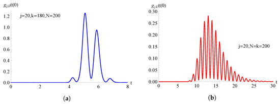
Figure 5. For the TNH-binomial birth process with $\lambda \left(t\right)=0.4[1+0.9cos(2\pi t\left)\right]$, the FPT pdf $g_{j,k}\left(t\right|0)$ is plotted as a function of t for $j=20$ and $N=200$. In (a) $k=180$ and in (b) $k=200$.

Remarks on the FPT Mean and Variance for the TH-Binomial Birth Process

For the TH-binomial birth process, with $\lambda \left(t\right)=\lambda$ and $t_0=0$, substituting ${\xi }_n=1$ into (36), one has the following:

$$\mathrm{E}\left[{\mathcal{T}}_{j,k}\right]=\frac{1}{\lambda }\sum _{i=j}^{k-1}\frac{1}{N-i},\mathrm{Var}\left[{\mathcal{T}}_{j,k}\right]=\frac{1}{{\lambda }^2}\sum _{i=j}^{k-1}\frac{1}{{(N-i)}^2},k=j+1,j+2,\dots ,N.$$

(51)

In Table 4, the mean $\mathrm{E}\left[{\mathcal{T}}_{j,k}\right]$, the variance $\mathrm{Var}\left[{\mathcal{T}}_{j,k}\right]$, and the coefficient of variation $\mathrm{Cv}\left[{\mathcal{T}}_{j,k}\right]=\sqrt{\mathrm{Var}\left[{\mathcal{T}}_{j,k}\right]}/\mathrm{E}\left[{\mathcal{T}}_{j,k}\right]$ of the FPT for the TH-binomial process are listed for $j=20$, $N=200$, $\lambda =0.4$, and for some choices of k. As shown in Table 4, the average time required for the entire population to become infected is $14.4324$.

Table 4. For the TH-binomial birth process, with ${\lambda }_n\left(t\right)=\lambda (N-n)$, the mean, the variance, and the coefficient of variation of the FPT are listed for $j=20$, $N=200$, $\lambda =0.4$, and for different values of k.

k	$\mathbf{E}\left[{\mathcal{T}}_{\mathit{j},\mathit{k}}\right]$	$\mathbf{Var}\left[{\mathcal{T}}_{\mathit{j},\mathit{k}}\right]$	$\mathbf{Cv}\left[{\mathcal{T}}_{\mathit{j},\mathit{k}}\right]$
40	0.293591	0.00431473	0.223735
60	0.626306	0.00985785	0.158527
80	1.01020	0.0172410	0.129979
100	1.46393	0.0275626	0.113407
120	2.01867	0.0430128	0.102739
140	2.73269	0.0686775	0.0958995
160	3.73601	0.119687	0.0926010
180	5.43802	0.270192	0.0955862
200	14.4324	10.2462	0.221791

For the TH-binomial birth process, now we are interested in the behavior of the mean and the variance of ${\mathcal{T}}_{j,N}$ for large population size. For this purpose, we denote by

$$H_n^{\left(m\right)}=\sum _{i=1}^n\frac{1}{i^m},n\in \mathbb{N},m=1,2,\dots$$

(52)

the generalized harmonic numbers and we assume that $H_0^{\left(m\right)}=0$ for $m>0$. In particular, by setting $m=1$ in (52), one obtains the harmonic numbers $H_n=H_n^{\left(1\right)}={\sum }_{i=1}^n(1/i)$.

For large population size, $\mathrm{E}\left[{\mathcal{T}}_{j,N}\right]$ and $\mathrm{Var}\left[{\mathcal{T}}_{j,N}\right]$ can be approximated using the following identities:

$$\underset{n\to +\infty }{lim}\left(H_n-lnn\right)=\gamma ,\underset{n\to +\infty }{lim}{H}_n^{\left(m\right)}=\zeta \left(m\right),m=1,2,\dots$$

(53)

where $\gamma =0.5772156649$ is the Euler–Mascheroni constant and $\zeta \left(m\right)={\sum }_{i=1}^{+\infty }(1/i^m)$ denotes the Riemann zeta function (cf. Abramowitz and Stegun [30], p. 807). Hence, recalling (51) and using (53), for large population size, the following approximations hold:

$$\begin{array}{cc}\hfill & \mathrm{E}\left[{\mathcal{T}}_{j,N}\right]=\frac{1}{\lambda }\sum _{k=1}^{N-j}\frac{1}{k}\simeq \frac{1}{\lambda }\left\{\gamma +ln(N-j)\right\}={\widehat{\mathrm{E}}}_{j,N},\hfill \\ \hfill & \mathrm{Var}\left[{\mathcal{T}}_{j,N}\right]=\frac{1}{{\lambda }^2}\sum _{k=1}^{N-j}\frac{1}{k^2}\simeq \frac{1}{{\lambda }^2}\frac{{\pi }^2}{6}={\widehat{\mathrm{V}}}_{j,N},\hfill \end{array}$$

(54)

being $\zeta \left(2\right)={\pi }^2/6$. We note that, for the TH-binomial birth process, $\mathrm{Var}\left[{\mathcal{T}}_{j,N}\right]$ admits a finite limit as $N\to +\infty$:

$$\underset{N\to +\infty }{lim}\mathrm{Var}\left[{\mathcal{T}}_{j,N}\right]=\frac{1}{{\lambda }^2}\frac{{\pi }^2}{6}·$$

In Table 5, the deterministic time $T^{*}$, given in (5) with ${\gamma }_1={\gamma }_2=1$, the mean $\mathrm{E}\left[{\mathcal{T}}_{j,N-1}\right]$, the mean $\mathrm{E}\left[{\mathcal{T}}_{j,N}\right]$, and the variance $\mathrm{Var}\left[{\mathcal{T}}_{j,N}\right]$, given in (51), and the asymptotic behaviors ${\widehat{\mathrm{E}}}_{j,N}$ and ${\widehat{\mathrm{V}}}_{j,N}$, given in (54), are listed for $j=20$, $\lambda =0.4$, and for increasing values of N. We observe a sufficient agreement between the values of $T^{*}$, obtained via the deterministic binomial model, and the values of $\mathrm{E}\left[{\mathcal{T}}_{j,N-1}\right]$, derived using the stochastic binomial birth process. Furthermore, a good agreement exists between the exact values of the FPT means and variances and their approximate values as N increases.

Table 5. For the TH-binomial birth process, with ${\lambda }_n\left(t\right)=\lambda (N-n)$, the deterministic time $T^{*}$, given in (5) with ${\gamma }_1={\gamma }_2=1$, the mean of ${\mathcal{T}}_{j,N-1}$, the mean and the variance of ${\mathcal{T}}_{j,N}$, and their asymptotic behaviors are listed for $j=20$, $\lambda =0.4$, and for different values of N.

N	${\mathit{T}}^{*}$	$\mathbf{E}\left[{\mathcal{T}}_{\mathit{j},\mathit{N}-1}\right]$	$\mathbf{E}\left[{\mathcal{T}}_{\mathit{j},\mathit{N}}\right]$	${\widehat{\mathbf{E}}}_{\mathit{j},\mathit{N}}$	$\mathbf{Var}\left[{\mathcal{T}}_{\mathit{j},\mathit{N}}\right]$	${\widehat{\mathbf{V}}}_{\mathit{j},\mathit{N}}$
50	8.50299	7.48747	9.98747	9.94603	10.0759	10.2808
100	10.9551	9.91370	12.4137	12.3981	10.2032	10.2808
200	12.9824	11.9324	14.4324	14.4254	10.2462	10.2808
300	14.0870	13.0345	15.5345	15.5300	10.2586	10.2808
400	14.8504	13.7968	16.2968	16.2935	10.2644	10.2808
500	15.4345	14.3801	16.8801	16.8775	10.2678	10.2808
1000	17.2189	16.1632	18.6632	18.6619	10.2745	10.2808
10000	23.0208	21.9640	24.4640	24.4639	10.2802	10.2808

4.2. Quadratic Birth Process

Let $M\left(t\right)$ be a TNH-quadratic birth process having birth intensity functions ${\lambda }_n\left(t\right)=\lambda \left(t\right){(N-n)}^2/N$ for $n=j,j+1,\dots ,N$. In this case, in (18) we set ${\xi }_n=(N-n)/N$.

Proposition 5.

For the TNH-quadratic birth process $M\left(t\right)$, one has the following:

$$\begin{array}{ccc}& & p_{j,n}\left(t\right|t_0)={\left[\frac{(N-j)!}{(N-n)!}\right]}^2\{\frac{(2N-2n)!}{(n-j)!(2N-j-n)!}{e}^{-[{(N-n)}^2/N]\Lambda \left(t\right|t_0)]}\hfill \\ & & +\sum _{r=j}^{n-1}{(-1)}^{n-r}\frac{2(N-r)}{2N-n-r}\frac{(2N-n-r)!e^{-[{(N-r)}^2/N]\Lambda \left(t\right|t_0)}}{(r-j)!(n-r)!(2N-j-r)!}\},n=j,j+1,\dots ,N.\hfill \end{array}$$

(55)

Proof. 

Equation (55) for $n=j$ immediately follows from (20). Moreover, since the assumptions of Proposition 1 are satisfied with ${\xi }_n=(N-n)/N$, from (26) for $r=j,j+1,\dots ,n-1$ one obtains

$$A_{j,n}^{\left(r\right)}=\left\{\begin{array}{cc}1,\hfill & n=j,\hfill \\ {\displaystyle {(-1)}^{n-r}{\left[\frac{(N-j)!}{(N-n)!}\right]}^2\frac{2(N-r)}{2N-n-r}\frac{(2N-n-r)!}{(r-j)!(n-r)!(2N-j-r)!},}\hfill & n=j+1,j+2,\dots ,N,\hfill \end{array}\right.$$

(56)

and, for $r=n$, this results in

$$A_{j,n}^{\left(n\right)}=\left\{\begin{array}{cc}1,\hfill & n=j,\hfill \\ {\displaystyle {\left[\frac{(N-j)!}{(N-n)!}\right]}^2\frac{(2N-2n)!}{(n-j)!(2N-j-n)!},}\hfill & n=j+1,j+2,\dots ,N.\hfill \end{array}\right.$$

(57)

From (57), we note that $A_{j,N}^{\left(N\right)}=1$. Making use of (56) and (57) in Equation (25), one obtains (55) for $n=j+1,j+2,\dots ,N$. □

For $k=j+1,j+2,\dots ,N$, the FPT pdf of the NTH-quadratic birth process is obtainable from (33) making use of (55):

$$\begin{array}{ccc}& & g_{j,k}\left(t\right|t_0)=\lambda \left(t\right)\frac{{(N-k+1)}^2}{N}{p}_{j,k-1}\left(t\right|t_0)\hfill \\ & & =\frac{2\lambda \left(t\right)}{N}{\left[\frac{(N-j)!}{(N-k)!}\right]}^2\sum _{r=j}^{k-1}{(-1)}^{k-1-r}(N-r)\frac{(2N-k-r)!e^{-[{(N-r)}^2/N]\Lambda \left(t\right|t_0)}}{(r-j)!(k-1-r)!(2N-j-r)!}·\hfill \end{array}$$

(58)

In Figure 6, we consider the TNH-quadratic birth process with $\lambda \left(t\right)=0.4[1+0.9cos(2\pi t/Q\left)\right]$, with $Q=5$; the FPT pdf $g_{j,k}\left(t\right|t_0)$, given in (58), is plotted as a function of t for $N=20$, $j=2$, and for $k=15$ on the left and $k=N=20$ on the right.

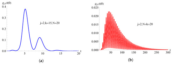
Figure 6. For the TNH-quadratic birth process with $\lambda \left(t\right)=0.4[1+0.9cos(2\pi t/Q\left)\right]$, with $Q=5$, the FPT pdf $g_{j,k}\left(t\right|0)$ is plotted as function of t for $j=2$ and $N=20$. In (a) $k=15$ and in (b) $k=20$.

Remarks on the FPT Mean and Variance for TH-Quadratic Birth Process

For the TH-quadratic birth process, with $\lambda \left(t\right)=\lambda$ and $t_0=0$, substituting ${\xi }_n=(N-n)/N$ into (36), one has

$$\mathrm{E}\left[{\mathcal{T}}_{j,k}\right]=\frac{N}{\lambda }\sum _{i=j}^{k-1}\frac{1}{{(N-i)}^2},\mathrm{Var}\left[{\mathcal{T}}_{j,k}\right]={\left(\frac{N}{\lambda }\right)}^2\sum _{i=j}^{k-1}\frac{1}{{(N-i)}^4},k=j+1,j+2,\dots ,N.$$

(59)

In Table 6, the mean $\mathrm{E}\left[{\mathcal{T}}_{j,k}\right]$, the variance $\mathrm{Var}\left[{\mathcal{T}}_{j,k}\right]$, and the coefficient of variation $\mathrm{Cv}\left[{\mathcal{T}}_{j,k}\right]$ of the FPT for the TH-quadratic birth process are listed for $j=20$, $N=200$, $\lambda =0.4$, and for some choices of k. As shown in Table 6, the average time required for the entire population to become infected is $819.697$.

Table 6. For the TH-quadratic birth process, with ${\lambda }_n\left(t\right)=\lambda {(N-n)}^2/N$, the mean, the variance, and the coefficient of variation of the FPT are listed for $j=20$, $N=200$, $\lambda =0.4$, and for different values of k.

k	$\mathbf{E}\left[{\mathcal{T}}_{\mathit{j},\mathit{k}}\right]$	$\mathbf{Var}\left[{\mathcal{T}}_{\mathit{j},\mathit{k}}\right]$	$\mathbf{Cv}\left[{\mathcal{T}}_{\mathit{j},\mathit{k}}\right]$
40	0.345179	0.00598477	0.224119
60	0.788628	0.0158751	0.159767
80	1.37928	0.0334555	0.132612
100	2.20501	0.0679213	0.118193
120	3.44102	0.145564	0.110876
140	5.49420	0.362094	0.109523
160	9.57498	1.23990	0.116293
180	21.6153	9.64726	0.143694
200	819.697	270581	0.634593

By comparing the results of Table 4 and Table 6, we note that the averages and the variances of the FPT for the TH-quadratic birth process are greater than those obtained for the TH-binomial birth process.

For the TH-quadratic birth process, we now take into account the behavior of the mean and the variance of ${\mathcal{T}}_{j,N}$ for large values of N. Recalling (59), for large population size, the following approximations hold:

$$\begin{array}{cc}\hfill & \mathrm{E}\left[{\mathcal{T}}_{j,N}\right]=\frac{N}{\lambda }\sum _{k=1}^{N-j}\frac{1}{k^2}\simeq \frac{N}{\lambda }\frac{{\pi }^2}{6}={\widehat{\mathrm{E}}}_{j,N},\hfill \\ \hfill & \mathrm{Var}\left[{\mathcal{T}}_{j,N}\right]={\left(\frac{N}{\lambda }\right)}^2\sum _{k=1}^{N-j}\frac{1}{k^4}\simeq {\left(\frac{N}{\lambda }\right)}^2\frac{{\pi }^2}{90}={\widehat{\mathrm{V}}}_{j,N},\hfill \end{array}$$

(60)

where (53) has been used with $\zeta \left(2\right)={\pi }^2/6$ and $\zeta \left(4\right)={\pi }^4/90$. Differently from the binomial birth process, for the quadratic birth process, the variance $\mathrm{Var}\left[{\mathcal{T}}_{j,N}\right]$ does not admit a finite limit and N increases.

In Table 7, the deterministic time $T^{*}$, given in (5) with ${\gamma }_1=0$ and ${\gamma }_2=1$, the mean $\mathrm{E}\left[{\mathcal{T}}_{j,N-1}\right]$, the mean $\mathrm{E}\left[{\mathcal{T}}_{j,N}\right]$, and the variance $\mathrm{Var}\left[{\mathcal{T}}_{j,N}\right]$, given in (59), and the asymptotic behaviors ${\widehat{\mathrm{E}}}_{j,N}$ and ${\widehat{\mathrm{V}}}_{j,N}$, given in (60), are listed for $j=20$, $\lambda =0.4$, and for increasing values of N. We observe a substantial discrepancy between the values of $T^{*}$, obtained via the deterministic quadratic model, and the values of $\mathrm{E}\left[{\mathcal{T}}_{j,N-1}\right]$, derived using the stochastic quadratic birth process. Instead, an excellent agreement exists between the exact values of the FPT means and variances and their approximate values as N increases.

Table 7. For the TH-quadratic birth process, with ${\lambda }_n\left(t\right)=\lambda {(N-n)}^2/N$, the deterministic time $T^{*}$, given in (5) with ${\gamma }_1=0$ and ${\gamma }_2=1$, the mean of ${\mathcal{T}}_{j,N-1}$, the mean and the variance of ${\mathcal{T}}_{j,N}$, and their asymptotic behaviors are listed for $j=20$, $\lambda =0.4$. and for different values of N.

N	${\mathit{T}}^{*}$	$\mathbf{E}\left[{\mathcal{T}}_{\mathit{j},\mathit{N}-1}\right]$	$\mathbf{E}\left[{\mathcal{T}}_{\mathit{j},\mathit{N}}\right]$	${\widehat{\mathbf{E}}}_{\mathit{j},\mathit{N}}$	$\mathbf{Var}\left[{\mathcal{T}}_{\mathit{j},\mathit{N}}\right]$	${\widehat{\mathbf{V}}}_{\mathit{j},\mathit{N}}$
50	120.833	76.5188	201.519	205.617	16,911.1	16,911.3
100	246.875	158.128	408.128	411.234	67,645.2	67,645.2
200	497.222	319.697	819.697	822.467	270,581	270,581
300	747.321	481.027	1231.03	1233.70	608,807	608,807
400	997.368	642.306	1642.31	1644.93	1,082,323	1,082,323
500	1247.40	803.566	2053.57	2056.17	1,691,130	1,691,130
1000	2497.45	1609.79	4109.79	4112.34	6,764,520	6,764,520
10,000	24,997.5	16,120.8	41,120.8	41,123.4	676,452,021	676,452,021

4.3. SI Birth Process

Let $M\left(t\right)$ be a TNH-SI birth process with birth intensity functions ${\lambda }_n\left(t\right)=(N-n)n\lambda \left(t\right)/N$ for $n=j,j+1,\dots ,N$. In this case, in (18), we set ${\xi }_n=n/N$. The TH-SI birth process, with $j=1$, is considered in studies by Allen [5] and Bailey [1,8,31]. The TNH-SI birth process, with $j=1$ and total population size $N+1$, is also taken in account in the study of Yang and Chiang [32,33].

For the SI birth process, considerable efforts are required to obtain general expressions of the transition probabilities $p_{j,n}\left(t\right|t_0)$ and of the FPT densities $g_{j,k}\left(t\right|t_0)$. In particular, for the TH-SI birth process, in which $t_0=0$ and $\lambda \left(t\right)=\lambda$, it is necessary to determine the inverse LT of (23), that is

$${\tilde{\Pi }}_{j,n}\left(s\right)=\frac{(N-j)!(n-1)!}{(N-n)!(j-1)!N^{n-j}}\frac{1}{Q_{j,n}\left(s\right)},n=j,j+1,\dots ,N,$$

(61)

where, due to (31),

$$Q_{j,n}\left(s\right)=\prod _{r=j}^n\left[s+\frac{(N-r)r}{N}\right],j\le n\le N,$$

(62)

is a polynomial in s of degree $n-j+1$, that depends on j, n, and N. For fixed j, n, and N, the roots of (62) can all be different or some of them are repeated twice. We remark that two roots $s_i=-(N-i)i/N$ and $s_k=-(N-k)k/N$, with $i,k=1,2,\dots ,n$ and $i\ne k$, are equal if and only if $N=i+k$. In the sequel, if the root $s_r=-(N-r)r/N$ of polynomial (62) is of single multiplicity, we define the coefficient

$$C_{j,n}^{\left(r\right)}=\underset{s\to -(N-r)r/N}{lim}\frac{[s+(N-r)r/N]}{Q_{j,n}\left(s\right)},$$

(63)

whereas, if $s_r$ is of multiplicity two, we consider the coefficients:

$$D_{j,n}^{(r,1)}=\underset{s\to -(N-r)r/N}{lim}\frac{{[s+(N-r)r/N]}^2}{Q_{j,n}\left(s\right)},D_{j,n}^{(r,2)}=\underset{s\to -(N-r)r/N}{lim}\frac{d}{ds}\frac{{[s+(N-r)r/N]}^2}{Q_{j,n}\left(s\right)}.$$

(64)

To determine the inverse LT of (61), we distinguish two cases: $N\le 2j$ and $N>2j$.

4.3.1. Case $N\le 2j$

Proposition 6.

For the TNH-SI birth process $M\left(t\right)$, the following results hold:

• For $N\le 2j-1$ one has the following:

  $$\begin{array}{ccc}& & p_{j,n}\left(t\right|t_0)=\frac{(N-j)!(n-1)!}{(N-n)!(j-1)!}\sum _{r=j}^n\frac{{(-1)}^{n-r}(2r-N)(j+r-N-1)!}{(r-j)!(n-r)!(n+r-N)!}{e}^{-[(N-r)r/N]\Lambda \left(t\right|t_0)},\hfill \\ & & n=j,j+1,\dots ,N;\hfill \end{array}$$

  (65)
• For $N=2j$, the result is as follows:

  $$\begin{array}{ccc}& & p_{j,n}\left(t\right|t_0)=\frac{j(n-1)!}{(2j-n)!}\frac{{(-1)}^{n-j}{e}^{-(j/2)\Lambda \left(t\right|t_0)}}{{[(n-j)!]}^2}\hfill \\ & & +\frac{2j(n-1)!}{(2j-n)!}\sum _{r=j+1}^n\frac{{(-1)}^{n-r}{e}^{-[(2j-r)r/\left(2j\right)]\Lambda \left(t\right|t_0)}}{(n-r)!(n+r-2j)!},n=j,j+1,\dots ,2j.\hfill \end{array}$$

  (66)

Proof. 

We assume that $N\le 2j$. For $i,k=j,j+1\dots ,N$, $i\ne k$, one has $N-i-k<N-2j\le 0$, so that $N-i-k<0$. Hence, the roots of polynomial (62) are all distinct for $j\le n\le N\le 2j$. The assumptions of Proposition 1 are satisfied, with ${\xi }_n=n/N$.

In particular, if $N\le 2j-1$, by virtue of (26), for $r=j,j+1,\dots ,n$ one obtains

$$A_{j,n}^{\left(r\right)}=\left\{\begin{array}{cc}1,\hfill & n=j,\hfill \\ {\displaystyle {(-1)}^{n-r}\frac{(N-j)!(n-1)!}{(N-n)!(j-1)!}\frac{(2r-N)(j+r-N-1)!}{(r-j)!(n-r)!(n+r-N)!},}\hfill & n=j+1,j+2,\dots ,N,\hfill \end{array}\right.$$

(67)

so that, making use of (67) in (25), we obtain (65) for $n=j,j+1,\dots ,N$.

Moreover, for $N=2j$, if $r=j$, the result is as follows:

$$A_{j,n}^{\left(j\right)}=\left\{\begin{array}{cc}1,\hfill & n=j,\hfill \\ {\displaystyle {(-1)}^{n-j}\frac{j(n-1)!}{(2j-n)!{[(n-j)!]}^2},}\hfill & n=j+1,j+2,\dots ,2j,\hfill \end{array}\right.$$

(68)

whereas, if $r=j+1,j+2,\dots ,2j$ one has the following:

$$A_{j,n}^{\left(r\right)}=\left\{\begin{array}{cc}1,\hfill & n=j,\hfill \\ {\displaystyle {(-1)}^{n-r}\frac{2j(n-1)!}{(2j-n)!(n-r)!(n+r-2j)!},}\hfill & n=j+1,j+2,\dots ,2j.\hfill \end{array}\right.$$

(69)

Hence, making use of (68) and (69) in (25), we obtain (66) for $n=j,j+1,\dots ,2j$. □

Under the assumptions of Proposition 6, by virtue of (33), the FPT pdf $g_{j,k}\left(t\right|t_0)$ of the TNH-SI birth process can be obtained. Indeed, from (65), for $N\le 2j-1$ and $k=j+1,j+2,\dots ,N$ one has the following:

$$\begin{array}{ccc}& & g_{j,k}\left(t\right|t_0)=\lambda \left(t\right)\frac{(N-k+1)(k-1)}{N}{p}_{j,k-1}\left(t\right|t_0)\hfill \\ & & =\frac{\lambda \left(t\right)(k-1)!(N-j)!}{N(j-1)!(N-k)!}\sum _{r=j}^{k-1}\frac{{(-1)}^{k-1-r}(2r-N)(j+r-N-1)!}{(r-j)!(k-1-r)!(k+r-N-1)!}{e}^{-[(N-r)r/N]\Lambda \left(t\right|t_0)},\hfill \end{array}$$

(70)

whereas for $N=2j$ and $k=j+1,j+2,\dots ,2j$ one obtains the following:

$$\begin{array}{ccc}& & g_{j,k}\left(t\right|t_0)=\lambda \left(t\right)\frac{(2j-k+1)(k-1)}{2j}{p}_{j,k-1}\left(t\right|t_0)\hfill \\ & & =\frac{\lambda \left(t\right)(k-1)!}{(2j-k)!}\left\{\frac{{(-1)}^{k-1-j}{e}^{-(j/2)\Lambda \left(t\right|t_0)}}{2{[(k-1-j)!]}^2}+\sum _{r=j+1}^{k-1}\frac{{(-1)}^{k-1-r}{e}^{-[(2j-r)r/\left(2j\right)]\Lambda \left(t\right|t_0)}}{(k-1-r)!(k-1+r-2j)!}\right\}·\hfill \end{array}$$

(71)

In Figure 7, we consider the TNH-SI birth process with $\lambda \left(t\right)=0.4[1+0.9cos(2\pi t\left)\right]$. In Figure 7a, the FPT pdf $g_{j,k}\left(t\right|t_0)$, given in (70), is plotted as a function of t for $N\le 2j-1$, with $j=10$, $k=15$, and $N=19$. Instead, in Figure 7b, the FPT pdf $g_{j,k}\left(t\right|t_0)$, given in (71), is plotted as a function of t for $N=2j$, with $j=10$, $k=15$, and $N=20$.

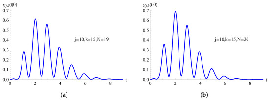
Figure 7. For the TNH-SI birth process with $\lambda \left(t\right)=0.4[1+0.9cos(2\pi t\left)\right]$, the FPT pdf $g_{j,k}\left(t\right|0)$ is plotted as a function of t for $j=10$ and $k=15$. In (a) $N=19$ and in (b) $N=20$.

4.3.2. Case $N>2j$

Let j, n, and N be fixed values, with $j\le n\le N$. When $N>2j$, it is necessary to distinguish the following cases:

• $N>2j$ and $j\le n\le N/2$ (see Proposition 7);
• $N>2j$, $N/2<n\le N$ and $n-j+1$ is odd (see Proposition 8);
• $N>2j$, $N/2<n\le N$ and $n-j+1$ is even (see Proposition 9).

Proposition 7.

Let j, n, and N be fixed values, with $N>2j$ and $j\le n\le N/2$. For the TNH-SI birth process, the result is as follows:

• If $j\le n<N/2$, one has the following:

  $$p_{j,n}\left(t\right|t_0)=\frac{(N-j)!(n-1)!}{(N-n)!(j-1)!}\sum _{r=j}^n\frac{{(-1)}^{r-j}(N-2r)(N-n-r-1)!}{(r-j)!(n-r)!(N-j-r)!}{e}^{-[(N-r)r/N]\Lambda \left(t\right|t_0)};$$

  (72)
• If $n=N/2$, one obtains the following:

  $$\begin{array}{ccc}& & p_{j,N/2}\left(t\right|t_0)=\frac{2(N-j)!}{N(j-1)!}\{2\sum _{r=j}^{N/2-1}\frac{{(-1)}^{r-j}}{(r-j)!(N-j-r)!}{e}^{-[(N-r)r/N]\Lambda \left(t\right|t_0)}\hfill \\ & & +\frac{{(-1)}^{N/2-j}}{{[(N/2-j)!]}^2}{e}^{-(N/4)\Lambda \left(t\right|t_0)}\}.\hfill \end{array}$$

  (73)

Proof. 

When j, n, and N are fixed values, with $N>2j$ and $j\le n\le N/2$, all the roots of the polynomial (62) have single multiplicity. Indeed, for each pair of distinct roots, $s_i$ and $s_k$, of (62), it results in $i+k<2n\le N$, so that $N-i-k>0$. From (63), for $j\le n<N/2$ one has the following:

$$C_{j,n}^{\left(r\right)}=\frac{N^{n-j}{(-1)}^{r-j}(N-2r)(N-n-r-1)!}{(r-j)!(n-r)!(N-j-r)!},r=j,j+1,\dots ,n,$$

whereas for $n=N/2$ one obtains the following:

$$C_{j,N/2}^{\left(r\right)}=\frac{2{(-1)}^{r-j}{N}^{N/2-j}}{(r-j)!(N-j-r)!},r=j,j+1,\frac{N}{2}-1,C_{j,N/2}^{(N/2)}=\frac{{(-1)}^{r-j}{N}^{N/2-j}}{{[(N/2-j)!]}^2}·$$

Hence, taking the inverse LT of (61), for j, n, and N fixed, with $N>2j$ and $j\le n\le N/2$, one obtains

$${\tilde{p}}_{j,n}\left(t\right)=\frac{(N-j)!(n-1)!}{(N-n)!(j-1)!N^{n-j}}\sum _{r=j}^n{C}_{j,n}^{\left(r\right)}{e}^{-\left[\right(N-r)r/N]t},$$

so that, by virtue of (21), Equations (72) and (73) follow. □

Note that (72) is in agreement with the result in the study of Yang and Chiang [32] for $t_0=0$, $j=1$, when the total population size is equal to $N+1$ and $\lambda \left(t\right)=(N+1)\beta \left(t\right)$.

Under the assumptions of Proposition 7, recalling (33), the FPT pdf $g_{j,k}\left(t\right|t_0)$ of the TNH-SI birth process can be obtained in the case $N>2j$ and $j+1\le k\le (N/2)+1$. Indeed, by virtue of (72), $N>2j$ and $j+1\le k<(N/2)+1$ one has the following:

$$g_{j,k}\left(t\right|t_0)=\frac{\lambda \left(t\right)(k-1)!(N-j)!}{N(j-1)!(N-k)!}\sum _{r=j}^{k-1}\frac{{(-1)}^{r-j}(N-2r)(N-k-r)!}{(r-j)!(k-1-r)!(N-j-r)!}{e}^{-[(N-r)r/N]\Lambda \left(t\right|t_0)},$$

(74)

whereas, for $N>2j$ and $k=N/2+1$, by using (73), one obtains the following:

$$\begin{array}{ccc}& & g_{j,N/2+1}\left(t\right|t_0)=\frac{\lambda \left(t\right)(N-j)!}{(j-1)!}\{\sum _{r=j}^{N/2-1}\frac{{(-1)}^{r-j}}{(r-j)!(N-j-r)!}{e}^{-[(N-r)r/N]\Lambda \left(t\right|t_0)}\hfill \\ & & +\frac{{(-1)}^{N/2-j}}{2{[(N/2-j)!]}^2}{e}^{-(N/4)\Lambda \left(t\right|t_0)}\}.\hfill \end{array}$$

(75)

In Figure 8, we consider the TNH-SI birth process with $\lambda \left(t\right)=0.4[1+0.9cos(2\pi t\left)\right]$. In Figure 8a, the FPT pdf $g_{j,k}\left(t\right|t_0)$, given in (74), is plotted as a function of t for $j=2$, $k=10$, and $N=20$. Instead, in Figure 8b, the FPT pdf $g_{j,k}\left(t\right|t_0)$, given in (75), is plotted as a function of t for $j=2$, $k=11$, and $N=20$.

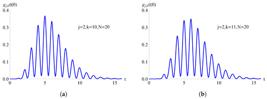
Figure 8. For the TNH-SI birth process with $\lambda \left(t\right)=0.4[1+0.9cos(2\pi t\left)\right]$, the FPT pdf $g_{j,k}\left(t\right|0)$ is plotted as function of t for $j=2$ and $N=20$. In (a) $k=10$ and in (b) $k=11$.

Proposition 8.

For the TNH-SI birth process, we assume that j, n, and N are fixed values, with $N>2j$, $N/2<n\le N$ and $n-j+1$ odd. Then,

$$p_{j,n}\left(t\right|t_0)=\left\{\begin{array}{c}{\displaystyle \frac{(N-j)!(n-1)!}{(N-n)!(j-1)!N^{n-j}}\{C_{j,n}^{\left(j\right)}{e}^{-[(N-j)j/N]\Lambda \left(t\right|t_0)}}\hfill \\ {\displaystyle +\sum _{r=j+1}^{(n+j)/2}\left[D_{j,n}^{(r,1)}\Lambda \left(t\right|t_0)+D_{j,n}^{(r,2)}\right]e^{-[(N-r)r/N]\Lambda \left(t\right|t_0)}\},}\hfill & n<N-j,\hfill \\ {\displaystyle \frac{(N-j)!(n-1)!}{(N-n)!(j-1)!N^{n-j}}\{\sum _{r=j}^{(N/2)-1}\left[D_{j,n}^{(r,1)}\Lambda \left(t\right|t_0)+D_{j,n}^{(r,2)}\right]e^{-[(N-r)r/N]\Lambda \left(t\right|t_0)}}\hfill \\ {\displaystyle +C_{j,n}^{(N/2)}{e}^{-(N/4)\Lambda \left(t\right|t_0)}\},}\hfill & n=N-j,\hfill \\ {\displaystyle \frac{(N-j)!(n-1)!}{(N-n)!(j-1)!N^{n-j}}\{\sum _{r=(n+j)/2}^{n-1}\left[D_{j,n}^{(r,1)}\Lambda \left(t\right|t_0)+D_{j,n}^{(r,2)}\right]e^{-[(N-r)r/N]\Lambda \left(t\right|t_0)}}\hfill \\ {\displaystyle +C_{j,n}^{\left(n\right)}{e}^{-[(N-n)n/N]\Lambda \left(t\right|t_0)}\},}\hfill & n>N-j,\hfill \end{array}\right.$$

(76)

where the coefficients $C_{j,n}^{\left(r\right)}$ and $D_{j,n}^{(r,\ell )}$$(\ell =1,2)$ are defined in (63) and (64), respectively.

Proof. 

Let $j,n$ and N be fixed values, with $N>2j$, $N/2<n\le N$, and $n-j+1$ odd. The polynomial (62) has $(n-j)/2$ roots of multiplicity two and one root of single multiplicity. From (62), one has the following:

$$Q_{j,n}\left(s\right)=\left\{\begin{array}{cc}{\displaystyle \left[s+\frac{(N-j)j}{N}\right]\prod _{r=j+1}^{(n+j)/2}{\left[s+\frac{(N-r)r}{N}\right]}^2,}\hfill & n<N-j,\hfill \\ {\displaystyle \prod _{r=j}^{(N/2)-1}{\left[s+\frac{(N-r)r}{N}\right]}^2\left(s+\frac{N}{4}\right),}\hfill & n=N-j,\hfill \\ {\displaystyle \prod _{r=(n+j)/2}^{n-1}{\left[s+\frac{(N-r)r}{N}\right]}^2\left[s+\frac{(N-n)n}{N}\right],}\hfill & n>N-j.\hfill \end{array}\right.$$

(77)

We note that, if $n<N-j$, one has $(N-j)j<(N-r)r$ for $r=j+1,\dots ,(n+j)/2$. Instead, $n=N-j$, it results in $N/4>(N-r)r/N$ for $r=j,j+1,\dots ,(N/2)-1$. Moreover, if $n>N-j$, we have $(N-n)n<(N-r)r$ for $r=(n+j)/2,\dots ,n-1$. Therefore, recalling (77) and making use of Proposition 2, Equation (76) follows. □

Proposition 9.

For the TNH-SI birth process, let j, n, and N be fixed values, with $N>2j$, $N/2<n\le N$, and $n-j+1$ even. Then,

$$p_{j,n}\left(t\right|t_0)=\left\{\begin{array}{c}{\displaystyle \frac{(N-j)!(n-1)!}{(N-n)!(j-1)!N^{n-j}}\{\sum _{r\notin U_1\cup U_2}{C}_{j,n}^{\left(r\right)}{e}^{-[(N-r)r/N]\Lambda \left(t\right|t_0)}}\hfill \\ {\displaystyle +\sum _{r\in U_1}\left[D_{j,n}^{(r,1)}\Lambda \left(t\right|t_0)+D_{j,n}^{(r,2)}\right]e^{-[(N-r)r/N]\Lambda \left(t\right|t_0)}\},}\hfill & n<N-j,\hfill \\ {\displaystyle \frac{(N-j)!(n-1)!}{(N-n)!(j-1)!N^{n-j}}\sum _{r=j}^{(N-1)/2}\left[D_{j,n}^{(r,1)}\Lambda \left(t\right|t_0)+D_{j,n}^{(r,2)}\right]e^{-[(N-r)r/N]\Lambda \left(t\right|t_0)},}\hfill & n=N-j,\hfill \\ {\displaystyle \frac{(N-j)!(n-1)!}{(N-n)!(j-1)!N^{n-j}}\{\sum _{r\in V_1}\left[D_{j,n}^{(r,1)}\Lambda \left(t\right|t_0)+D_{j,n}^{(r,2)}\right]e^{-[(N-r)r/N]\Lambda \left(t\right|t_0)}}\hfill \\ {\displaystyle +\sum _{r\notin V_1\cup V_2}{C}_{j,n}^{\left(r\right)}{e}^{-[(N-r)r/N]\Lambda \left(t\right|t_0)}\},}\hfill & n>N-j,\hfill \end{array}\right.$$

(78)

where the coefficients $C_{j,n}^{\left(r\right)}$ and $D_{j,n}^{(r,\ell )}$$(\ell =1,2)$ are defined in (63) and (64) and

$$\begin{array}{cc}\hfill & U_1=\left\{\frac{n+j+3}{2},\dots ,n\right\},U_2=\left\{N-n,\dots ,N-\frac{n+j+3}{2}\right\},\hfill \\ \hfill & V_1=\left\{j,\dots ,\frac{n+j-3}{2}\right\},V_2=\left\{N-\frac{n+j-3}{2},\dots ,N-j\right\},\hfill \end{array}$$

(79)

Proof. 

Let $N>2j$, $N/2<n\le N$, and $n-j+1$ even. The cardinality of $U_1\cup U_2$ and of $V_1\cup V_2$ is $n-j-1$. If $n\ne N-j$, in the polynomial (62) there are $(n-j-1)/2$ roots of multiplicity two and two roots of single multiplicity. Instead, if $n=N-j$, the roots of polynomial (62) all have multiplicity two. Indeed, in a fixed root $s_i$, with $j\le i\le n$, there always exists another equal root $s_{N-i}$ with $j=N-n\le N-i\le N-j=n$, being $N=n+j$. From (62), one has the following:

$$Q_{j,n}\left(s\right)=\left\{\begin{array}{cc}{\displaystyle \prod _{r\notin U_1\cup U_2}\left[s+\frac{(N-r)r}{N}\right]\prod _{r\in U_1}{\left[s+\frac{(N-r)r}{N}\right]}^2,}\hfill & n<N-j,\hfill \\ {\displaystyle \prod _{r=j}^{(N-1)/2}{\left[s+\frac{(N-r)r}{N}\right]}^2,}\hfill & n=N-j,\hfill \\ {\displaystyle \prod _{r\in V_1}{\left[s+\frac{(N-r)r}{N}\right]}^2\prod _{r\notin V_1\cup V_2}\left[s+\frac{(N-r)r}{N}\right],}\hfill & n>N-j,\hfill \end{array}\right.$$

(80)

with $U_1,U_2$ and $V_1,V_2$ defined in (79). Therefore, recalling (80) and making use of Proposition 2, Equation (78) follows. □

We remark that, due to (61), for the TH-SI birth process, the following function in Mathematica

$$\frac{Factorial[N-j]Factorial[n-1]}{Factorial[N-n]Factorial[j-1]N^{n-j}}InverseLaplaceTransform\left[\frac{1}{Product\left[s+\frac{(N-i)i}{N},\{i,j,n\}\right]},s,t\right]$$

immediately gives the symbolic inverse LT ${\tilde{p}}_{j,n}\left(t\right)$ of ${\tilde{\Pi }}_{j,n}\left(s\right)$, with $j\le n\le N$.

For the TNH-SI birth process with $\lambda \left(t\right)=0.4[1+0.9cos(2\pi t\left)\right]$, in Figure 9 we plot the FPT pdf $g_{j,k}\left(t\right|t_0)=\lambda \left(t\right)[(N-k+1)(k-1)/N]p_{j,k-1}\left(t\right|0)$ as a function of t for $j=2$, $N=20$, and $k=15,20$. In these cases, the probabilities $p_{j,k-1}\left(t\right|0)$ have been obtained making use of relation (21) and of the inverse LT of Mathematica.

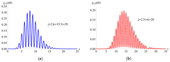
Figure 9. For the TNH-SI birth process with $\lambda \left(t\right)=0.4[1+0.9cos(2\pi t\left)\right]$, the FPT pdf $g_{j,k}\left(t\right|0)$ is plotted as function of t for $j=2$ and $N=20$. In (a) $k=15$ and in (b) $k=20$.

Remarks on the FPT Mean and Variance for the TH-SI Birth Process

For the TH-SI birth process, with $\lambda \left(t\right)=\lambda$ and $t_0=0$, substituting ${\xi }_n=n/N$ into (36), one has

$$\mathrm{E}\left[{\mathcal{T}}_{j,k}\right]=\frac{N}{\lambda }\sum _{i=j}^{k-1}\frac{1}{(N-i)i},\mathrm{Var}\left[{\mathcal{T}}_{j,k}\right]={\left(\frac{N}{\lambda }\right)}^2\sum _{i=j}^{k-1}\frac{1}{{\left[(N-i)i\right]}^2},k=j+1,j+2,\dots ,N.$$

(81)

In Table 8, the mean $\mathrm{E}\left[{\mathcal{T}}_{j,k}\right]$, the variance $\mathrm{Var}\left[{\mathcal{T}}_{j,k}\right]$, and the coefficient of variation $\mathrm{Cv}\left[{\mathcal{T}}_{j,k}\right]$ of the FPT for the TH-SI birth process are listed for $j=20$, $N=200$, $\lambda =0.4$, and for some choices of k. As shown in Table 8, the average time required for the entire population to become infected is $20.2456$.

Table 8. For the TH-SI birth process, with ${\lambda }_n\left(t\right)=\lambda (N-n)n/N$, the mean, the variance, and the coefficient of variation of the FPT are listed for $j=20$, $N=200$, $\lambda =0.4$, and for different values of k.

k	$\mathbf{E}\left[{\mathcal{T}}_{\mathit{j},\mathit{k}}\right]$	$\mathbf{Var}\left[{\mathcal{T}}_{\mathit{j},\mathit{k}}\right]$	$\mathbf{Cv}\left[{\mathcal{T}}_{\mathit{j},\mathit{k}}\right]$
40	2.05810	0.217990	0.226857
60	3.41497	0.310635	0.163207
80	4.52330	0.372151	0.134867
100	5.53802	0.423642	0.117529
120	6.55066	0.474921	0.105202
140	7.65155	0.535606	0.0956474
160	8.98982	0.625690	0.0879891
180	10.9872	0.830494	0.0829437
200	20.2456	11.04150	0.164128

For the TH-SI birth process, we consider the behavior of the mean and the variance of ${\mathcal{T}}_{j,N}$ for large population size. By virtue of (81), for large N, the following approximations hold:

$$\begin{array}{cc}\hfill & \mathrm{E}\left[{\mathcal{T}}_{j,N}\right]=\frac{1}{\lambda }\left\{\sum _{i=j}^{N-1}\frac{1}{i}+\sum _{i=1}^{N-j}\frac{1}{i}\right\}\simeq \frac{1}{\lambda }\left\{2\gamma -H_{j-1}+log\left[(N-1)(N-j)\right]\right\}={\widehat{E}}_{j,N},\hfill \\ \hfill & \mathrm{Var}\left[{\mathcal{T}}_{j,N}\right]=\frac{1}{{\lambda }^2}\left\{\sum _{i=j}^{N-1}\frac{1}{i^2}+\sum _{i=1}^{N-j}\frac{1}{i^2}+\frac{2\lambda }{N}\mathrm{E}\left[{\mathcal{T}}_{j,N}\right],\right\},\hfill \\ \hfill & \simeq \frac{1}{{\lambda }^2}\{\frac{{\pi }^2}{3}-H_{j-1}^{\left(2\right)}+\frac{2}{N}\left[2\gamma -H_{j-1}+log\left[(N-1)(N-j)\right]\right]\}={\widehat{V}}_{j,N},\hfill \end{array}$$

(82)

where (53) has been used with $\zeta \left(2\right)={\pi }^2/6$. Similarly to the binomial birth process, the variance of ${\mathcal{T}}_{j,N}$ has a finite limit for $N\to +\infty$:

$$\underset{N\to +\infty }{lim}\mathrm{Var}\left[{\mathcal{T}}_{j,N}\right]=\frac{1}{{\lambda }^2}\left\{\frac{{\pi }^2}{3}-H_{j-1}^{\left(2\right)}\right\}.$$

Results (81) and (82) are in agreement with those obtained in Allen’s study [5] for $j=1$.

In Table 9, the deterministic time $T^{*}$, given in (5) with ${\gamma }_1=1$ and ${\gamma }_2=0$, the mean $\mathrm{E}\left[{\mathcal{T}}_{j,N-1}\right]$, the mean $\mathrm{E}\left[{\mathcal{T}}_{j,N}\right]$, and the variance $\mathrm{Var}\left[{\mathcal{T}}_{j,N}\right]$, given in (81), and their asymptotic behaviors ${\widehat{\mathrm{E}}}_{j,N}$ and ${\widehat{\mathrm{V}}}_{j,N}$, given in (82), are listed for $j=20$, $\lambda =0.4$, and for increasing values of N. As for the binomial birth process, we observe a sufficient agreement between the values of $T^{*}$, obtained via the deterministic SI model, and the values of $\mathrm{E}\left[{\mathcal{T}}_{j,N-1}\right]$, derived using the stochastic SI birth process. Furthermore, a good agreement exists between the exact values of the FPT means and variances and their approximate values as N increases.

Table 9. For the TH-SI birth process, with ${\lambda }_n\left(t\right)=\lambda (N-n)n/N$, the deterministic time $T^{*}$, given in (5) with ${\gamma }_1=1$ and ${\gamma }_2=0$, the mean of ${\mathcal{T}}_{j,N-1}$, the mean and the variance of ${\mathcal{T}}_{j,N}$, and their asymptotic behaviors are listed for $j=20$, $\lambda =0.4$, and for different values of N.

N	${\mathit{T}}^{*}$	$\mathbf{E}\left[{\mathcal{T}}_{\mathit{j},\mathit{N}-1}\right]$	$\mathbf{E}\left[{\mathcal{T}}_{\mathit{j},\mathit{N}}\right]$	${\widehat{\mathbf{E}}}_{\mathit{j},\mathit{N}}$	$\mathbf{Var}\left[{\mathcal{T}}_{\mathit{j},\mathit{N}}\right]$	${\widehat{\mathbf{V}}}_{\mathit{j},\mathit{N}}$
50	10.7432	9.76511	12.3161	12.2493	11.5017	11.8262
100	14.9535	13.9625	16.4878	16.4596	11.2852	11.4243
200	18.7263	17.7330	20.2456	20.2324	11.0415	11.1071
300	20.8488	19.8551	22.3635	22.3548	10.9309	10.9739
400	22.3335	21.3397	23.8460	23.8396	10.8673	10.8993
500	23.4766	22.4828	24.9878	24.9827	10.8256	10.8511
1000	26.9964	26.0025	28.5050	28.5025	10.7312	10.7438
10000	38.5571	37.5632	40.0634	40.0632	10.6201	10.6213

For the TH-binomial, TH-quadratic, and TH-SI birth process, Table 5, Table 7, and Table 9 show that the deterministic time $T^{*}$ is always included in the interval $\left(\mathrm{E}\left[{\mathcal{T}}_{j,N-1}\right],\mathrm{E}\left[{\mathcal{T}}_{j,N}\right]\right)$.

5. Stochastic Hyper-Logistic Birth Process

Let $M\left(t\right)$ be a TNH-hyper-logistic birth process, having birth intensity functions ${\lambda }_n\left(t\right)=\lambda \left(t\right){(N-n)}^{1+p}{n}^{1-p}/N$, with $0\le p\le 1$ and $n=j,j+1,\dots ,N$. In this case, in (18), we set ${\xi }_n={(N-n)}^p{n}^{1-p}/N$. Note that the hyper-logistic birth process identifies with the SI birth process when $p=0$ and it becomes the quadratic birth process by setting $p=1$. Hence, in the sequel, we assume that $0<p<1$.

Proposition 10.

For the TNH-hyper-logistic birth process $M\left(t\right)$, with $0<p<1$, one has the following:

$$\begin{array}{ccc}& & p_{j,j}\left(t\right|t_0)=exp\left\{-\frac{{(N-j)}^{1+p}{j}^{1-p}}{N}\Lambda \left(t\right|t_0)\right\},\hfill \\ & & \hfill \\ & & {\displaystyle p_{j,n}\left(t\right|t_0)={\left[\frac{(N-j)!}{(N-n)!}\right]}^{1+p}{\left[\frac{(n-1)!}{(j-1)!}\right]}^{1-p}\sum _{r=j}^n\frac{exp\left\{-\frac{{(N-r)}^{1+p}{r}^{1-p}}{N}\Lambda \left(t\right|t_0)\right\}}{{\displaystyle \prod _{\begin{array}{c}i=j\\ i\ne r\end{array}}^n\left[{(N-i)}^{1+p}{i}^{1-p}-{(N-r)}^{1+p}{r}^{1-p}\right]}},n=j+1,j+2,\dots ,N.}\hfill \end{array}$$

(83)

Proof. 

The first equation in (83) immediately follows from (20). Moreover, if $0<p<1$, the assumptions of Proposition 1 are satisfied with ${\xi }_n={(N-n)}^p{n}^{1-p}/N$. Indeed, recalling (24), for $0<p<1$ one has

$${\left(\frac{N-i}{i}\right)}^p(N-i)i\ne {\left(\frac{N-k}{k}\right)}^p(N-k)k,i,k=j,j+1,\dots ,N-1,i\ne k.$$

Hence, making use of (26), for $r=j,j+1,\dots ,n$ one obtains

$$A_{j,n}^{\left(r\right)}=\left\{\begin{array}{cc}1,\hfill & n=j,\hfill \\ {\displaystyle \frac{{\left[\frac{(N-j)!}{(N-n)!}\right]}^{1+p}{\left[\frac{(n-1)!}{(j-1)!}\right]}^{1-p}}{{\displaystyle \prod _{\begin{array}{c}i=j\\ i\ne r\end{array}}^n\left[{(N-i)}^{1+p}{i}^{1-p}-{(N-r)}^{1+p}{r}^{1-p}\right]}}}\hfill & n=j+1,j+2,\dots ,N,\hfill \end{array}\right.$$

so that the second equation in (83) follows from (25).  □

The FPT pdf of the hyper-logistic birth process is obtainable from (33) by using (83):

$$\begin{array}{ccc}& & g_{j,j+1}\left(t\right|t_0)=\frac{\lambda \left(t\right)}{N}{(N-j)}^{1+p}{j}^{1-p}exp\left\{-\frac{{(N-j)}^{1+p}{j}^{1-p}}{N}\Lambda \left(t\right|t_0)\right\},\hfill \\ & & \hfill \\ & & {\displaystyle g_{j,k}\left(t\right|t_0)=\frac{\lambda \left(t\right)}{N}{\left[\frac{(N-j)!}{(N-k)!}\right]}^{1+p}{\left[\frac{(k-1)!}{(j-1)!}\right]}^{1-p}\sum _{r=j}^{k-1}\frac{exp\left\{-\frac{{(N-r)}^{1+p}{r}^{1-p}}{N}\Lambda \left(t\right|t_0)\right\}}{{\displaystyle \prod _{\begin{array}{c}i=j\\ i\ne r\end{array}}^{k-1}\left[{(N-i)}^{1+p}{i}^{1-p}-{(N-r)}^{1+p}{r}^{1-p}\right]}},k=j+2,j+3,\dots ,N.}\hfill \end{array}$$

(84)

In Figure 10, we consider the TNH-hyper-logistic birth process with $p=0.3$ and $\lambda \left(t\right)=0.4[1+0.9cos(2\pi t/Q\left)\right]$, with $Q=1$; the FPT pdf $g_{j,k}\left(t\right|t_0)$, given in (84), is plotted as function of t for $N=20$, $j=2$, and for $k=15$ on the left and $k=N=20$ on the right.

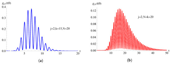
Figure 10. For the TNH-hyper-logistic birth process with $p=0.3$ and $\lambda \left(t\right)=0.4[1+0.9cos(2\pi t\left)\right]$, the FPT pdf $g_{j,k}\left(t\right|0)$ is plotted as function of t for $j=2$ and $N=20$. In (a) $k=15$ and in (b) $k=20$.

In Figure 11, we consider the TNH-hyper-logistic birth process with $p=0.7$ and $\lambda \left(t\right)=0.4[1+0.9cos(2\pi t/Q\left)\right]$, with $Q=5$; the FPT pdf $g_{j,k}\left(t\right|t_0)$, given in (84), is plotted as a function of t for $N=20$, $j=2$, and for $k=15$ on the left and $k=N=20$ on the right.

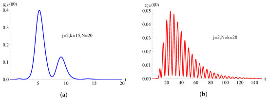
Figure 11. For the TNH-hyper-logistic birth process with $p=0.7$, $\lambda \left(t\right)=0.4[1+0.9cos(2\pi t/Q\left)\right]$, with $Q=5$, the FPT pdf $g_{j,k}\left(t\right|0)$ is plotted as function of t for $j=2$ and $N=20$. In (a) $k=15$ and in (b) $k=20$.

Remarks on the FPT Mean and Variance for the TH-Hyper-Logistic Birth Process

For the TH-hyper-logistic birth process, with $\lambda \left(t\right)=\lambda$ and $t_0=0$, substituting ${\xi }_n={(N-n)}^p{n}^{1-p}/N$ into (36), for $0<p<1$ one has the following:

$$\mathrm{E}\left[{\mathcal{T}}_{j,k}\right]=\frac{N}{\lambda }\sum _{i=j}^{k-1}\frac{1}{{(N-i)}^{1+p}{i}^{1-p}},\mathrm{Var}\left[{\mathcal{T}}_{j,k}\right]={\left(\frac{N}{\lambda }\right)}^2\sum _{i=j}^{k-1}\frac{1}{{\left[{(N-i)}^{1+p}{i}^{1+p}\right]}^2},k=j+1,j+2,\dots ,N.$$

(85)

In Table 10, the mean $\mathrm{E}\left[{\mathcal{T}}_{j,k}\right]$, the variance $\mathrm{Var}\left[{\mathcal{T}}_{j,k}\right]$, and the coefficient of variation $\mathrm{Cv}\left[{\mathcal{T}}_{j,k}\right]$ of the FPT for the TH-hyper-logistic birth process are listed for $j=20$, $N=200$, $\lambda =0.4$, and for different values of k, with $p=0.3$ (on the left) and $p=0.7$ (on the right). As shown in Table 10, the average time required for the entire population to become infected is $43.8655$ if $p=0.3$ and $208.389$ when $p=0.7$.

Table 10. For the TH-hyper-logistic birth process, with ${\lambda }_n\left(t\right)=\lambda {(N-n)}^{1+p}{n}^{1-p}/N$ the mean, the variance, and the coefficient of variation of the FPT are listed for $j=20$, $N=200$, $\lambda =0.4$, and for different values of p and k.

	$\mathit{p}=0.3$			$\mathit{p}=0.7$
$\mathit{k}$	$\mathrm{E}\left[{\mathcal{T}}_{\mathit{j},\mathit{k}}\right]$	$\mathrm{Var}\left[{\mathcal{T}}_{\mathit{j},\mathit{k}}\right]$	$\mathrm{Cv}\left[{\mathcal{T}}_{\mathit{j},\mathit{k}}\right]$	$\mathrm{E}\left[{\mathcal{T}}_{\mathit{j},\mathit{k}}\right]$	$\mathrm{Var}\left[{\mathcal{T}}_{\mathit{j},\mathit{k}}\right]$	$\mathrm{Cv}\left[{\mathcal{T}}_{\mathit{j},\mathit{k}}\right]$
40	1.19754	0.0724041	0.224693	0.586319	0.0171893	0.223612
60	2.16519	0.119272	0.159505	1.20496	0.0363428	0.158211
80	3.08125	0.161231	0.130316	1.91714	0.0617673	0.129636
100	4.03376	0.206619	0.112687	2.79428	0.100423	0.113409
120	5.10727	0.264364	0.100673	3.95689	0.168593	0.103768
140	6.43227	0.352653	0.092323	5.65705	0.315452	0.0992835
160	8.29745	0.529273	0.087679	8.57046	0.754576	0.101356
180	11.7024	1.14076	0.091269	15.5559	3.45829	0.119546
200	43.8655	198.557	0.321233	208.389	11893.5	0.523335

In Figure 12, the mean $\mathrm{E}\left[{\mathcal{T}}_{j,k}\right]$ and the coefficient of variation $\mathrm{Cv}\left[{\mathcal{T}}_{j,k}\right]$ of the FPT for the TH-hyper-logistic birth process are plotted as functions of $p\in (0,1)$ for $j=20$, $N=200$, $\lambda =0.4$, and for different values of k. We note that the behavior of the FPT mean and of the FPT coefficient of variation as a function of p depends on $k=j+1,j+2,\dots ,N$.

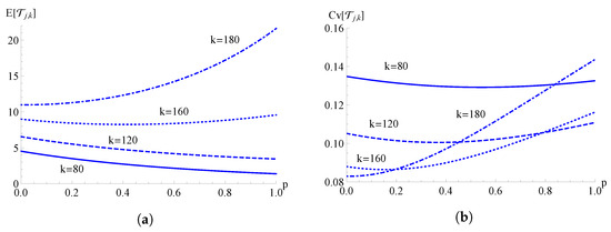
Figure 12. For the TH-hyper-logistic birth process, the mean in (a) and the coefficient of variation in (b) of the FPT are plotted as functions of $p\in (0,1)$ for $j=20$, $N=200$, $\lambda =0.4$, and for different values of k.

In Table 11, the deterministic time $T^{*}$, given in (16), the mean $\mathrm{E}\left[{\mathcal{T}}_{j,N-1}\right]$ and the mean $\mathrm{E}\left[{\mathcal{T}}_{j,N}\right]$, given in (85), are listed for $j=20$, $\lambda =0.4$, and for increasing values of N, with $p=0.3$ (on the left) and $p=0.7$ (on the right). We note that, as shown for the TH-binomial, in the TH-quadratic and TH-SI process, even for the TH-hyper-logistic birth processes, the deterministic time $T^{*}$ is always included in the interval $\left(\mathrm{E}\left[{\mathcal{T}}_{j,N-1}\right],\mathrm{E}\left[{\mathcal{T}}_{j,N}\right]\right)$.

Table 11. For the TH-hyper-logistic birth process, the deterministic time $T^{*}$, given in (16), the mean of ${\mathcal{T}}_{j,N-1}$ and of ${\mathcal{T}}_{j,N}$ are listed for $j=20$, $\lambda =0.4$, and for different values of p and N.

	$\mathit{p}=0.3$			$\mathit{p}=0.7$
$\mathit{N}$	${\mathit{T}}^{*}$	$\mathrm{E}\left[{\mathcal{T}}_{\mathit{j},\mathit{N}-\mathbf{1}}\right]$	$\mathrm{E}\left[{\mathcal{T}}_{\mathit{j},\mathit{N}}\right]$	${\mathit{T}}^{*}$	$\mathrm{E}\left[{\mathcal{T}}_{\mathit{j},\mathit{N}-\mathbf{1}}\right]$	$\mathrm{E}\left[{\mathcal{T}}_{\mathit{j},\mathit{N}}\right]$
50	19.4052	16.1976	24.3968	51.7587	37.2634	76.1546
100	27.5778	23.6011	33.6241	87.7280	64.1692	127.156
200	36.4719	31.5692	43.8655	144.457	106.221	208.389
300	42.3053	36.7659	50.6364	192.550	141.787	277.418
400	46.802	40.7617	55.8736	235.878	173.803	339.651
500	50.5221	44.0623	60.2148	275.998	203.439	397.296
1000	63.5814	55.624	75.4961	449.067	331.231	646.057
10,000	130.778	114.883	154.508	2253.22	1662.80	3240.24

6. Results and Discussion

In this paper, we have considered a finite population of total size N in which an individual can be in one of two states, either susceptible (S) or infectious (I). Specifically, we have described the growth of the infected population, making use of deterministic dynamics via stochastic birth processes. In the deterministic epidemic models with two states, we have introduced the transmission intensity function $\lambda \left(t\right)$ and an interaction term of the form $S\left(t\right)\phi \left[I\right(t\left)\right]$, where the dependence on the number of infected individuals occurs via a linear or nonlinear bounded function $\phi \left[I\right(t\left)\right]$. In the flexible model $\phi \left[I\left(t\right)\right]=[{\gamma }_{1}I\left(t\right)+{\gamma }_2[N-I\left(t\right)]/N$, with ${\gamma }_1\ge 0$, ${\gamma }_2\ge 0$, ${\gamma }_1+{\gamma }_2>0$. Special cases of the flexible model are the binomial model $({\gamma }_1={\gamma }_2=1)$, the quadratic model $({\gamma }_1=0,{\gamma }_2=1)$, and the SI model $({\gamma }_1=1,{\gamma }_2=0)$. The SI model leads to the Verhulst logistic growth curve for $I\left(t\right)$. Instead, in the hyper-logistic model $\phi \left[I\left(t\right)\right]={\left[I\left(t\right)\right]}^{1-p}{[N-I\left(t\right)]}^p/N$, with $0<p<1$. In general, the intensity function $\lambda \left(t\right)$, the parameters ${\gamma }_1$ and ${\gamma }_2$ in the flexible model, and the parameter p in the hyper-logistic model must be estimated by using real data related to the infection under consideration. We have analyzed the following TNH deterministic models and the corresponding stochastic finite birth processes: flexible, binomial, quadratic, SI, and hyper-logistic. We have determined the probability distribution of the number of infected individuals as a function of time, the expected duration until the infected population size reaches N, and we have obtained some asymptotic approximations for large values of N.

The study, carried out on deterministic and stochastic models, highlighted the following results:

• In the deterministic model, if ${lim}_{t\to +\infty }\Lambda \left(t\right|t_0)=+\infty$, at the end, all individuals of the population are infected, i.e., ${lim}_{t\to +\infty }I\left(t\right)=N$. In the stochastic finite birth process, describing the infected population, the state N is an absorbing boundary, so that if ${lim}_{t\to +\infty }\Lambda \left(t\right|t_0)=+\infty$ the process reaches the absorbing state in finite mean time.
• For the finite birth processes $M\left(t\right)$, we have determined the transition probabilities since their knowledge allows us to obtain the FPT densities and related moments.
• For the binomial birth process, the conditional mean $\mathrm{E}\left[M\left(t\right)\right|M\left(t_0\right)=j]$ identifies with the deterministic solution of the deterministic binomial birth model.
• For the flexible birth process, we have proved that $\mathrm{E}\left[M\left(t\right)\right|M\left(t_0\right)=j]\simeq NH\left(t\right)$ for large N, with $H\left(t\right)={lim}_{N\to +\infty }I\left(t\right)/N$.
• In the TH-deterministic model, we have calculated the duration $T^{*}$ required until $N-1$ individuals of a population are infected. Such parameters have been compared with the FPT averages $\mathrm{E}\left[{\mathcal{T}}_{j,N-1}\right]$ and $\mathrm{E}\left[{\mathcal{T}}_{j,N}\right]$ of the related finite birth process. Numerical computations have shown that the deterministic time $T^{*}$ is always included in the interval $\left(\mathrm{E}\left[{\mathcal{T}}_{j,N-1}\right],\mathrm{E}\left[{\mathcal{T}}_{j,N}\right]\right)$. We have observed a substantial discrepancy between the values of $T^{*}$ of the deterministic quadratic model and the average values in the quadratic birth process.
• For the TH-binomial, TH-quadratic, and TH-SI birth processes, we have obtained some asymptotic behaviors of the mean and variance of ${\mathcal{T}}_{j,N}$ for large N. Specifically, for large N one has the following:

  -

  For the TH-binomial birth process, $\mathrm{E}\left[{\mathcal{T}}_{j,N}\right]$ grows as $log(N-j)$, whereas the $\mathrm{Var}\left[{\mathcal{T}}_{j,N}\right]$ admits a finite limit as N increases;

  -

  For the TH-quadratic birth process, $\mathrm{E}\left[{\mathcal{T}}_{j,N}\right]$ grows linearly with N, whereas the $\mathrm{Var}\left[{\mathcal{T}}_{j,N}\right]$ grows quadratically with N;

  -

  For the TH-SI birth process, $\mathrm{E}\left[{\mathcal{T}}_{j,N}\right]$ grows as $log\left[\right(N-1\left)\right(N-j\left)\right]$ and the $\mathrm{Var}\left[{\mathcal{T}}_{j,N}\right]$ admits a finite limit as N increases.

• For the TH-hyper-logistic birth process, we have studied the behavior of the mean and coefficient of variation of FPT as functions of $p\in (0,1)$ for various choices of the state k, with $j<k\le N$; for k near to the initial state j, $\mathrm{E}\left[{\mathcal{T}}_{j,k}\right]$ is a decreasing function of p, whereas for k near to N the mean, $\mathrm{E}\left[{\mathcal{T}}_{j,k}\right]$ is an increasing function of p.

The results obtained can help in choosing a suitable model to study real data and make predictions on the possible developments of the epidemics.

References

- Bailey, N.T.J. The Elements of Stochastic Processes with Applications to the Natural Sciences; John Wiley & Sons, Inc.: New York, NY, USA, 1964. [Google Scholar]
- Bharucha-Reid, A.T. Elements of the Theory of Markov Processes and Their Applications; McGraw-Hill: New York, NY, USA, 1960. [Google Scholar]
- Cox, D.R.; Miller, H.D. The Theory of Stochastic Processes; Chapman & Hall/CRC: Boca Raton, FL, USA, 1996. [Google Scholar]
- Taylor, H.M.; Karlin, S. An Introduction to Stochastic Modeling; Academic Press: San Diego, CA, USA, 1998. [Google Scholar]
- Allen, L.J.S. An Introduction to Stochastic Processes with Applications to Biology; Chapman and Hall/CRC: Lubbock, TX, USA, 2010. [Google Scholar]
- Allen, L.J.S. Stochastic Population and Epidemic Models. Persistence and Extinction; Springer International Publishing: Cham, Switzerland, 2015. [Google Scholar]
- Dailey, D.J.; Gani, J. Epidemic Modelling: An Introduction; Cambridge University Press: Cambridge, UK, 1999. [Google Scholar]
- Bailey, N.T.J. The Mathematical Theory of Epidemics; Charles Griffin and Co. Ltd.: Glasgow, UK, 1957. [Google Scholar]
- Anggriani, N.; Panigoro, H.S.; Rahmi, E.; Peter, O.J.; Jose, S.A. A predator-prey model with additive Allee effect and intraspecific competition on predator involving Atangana-Balenu-Caputo derivative. Results Physic 2023, 49, 106489. [Google Scholar] [CrossRef]
- Joseph, D.; Ramachandran, R.; Alzabut, J.; Jose, S.A.; Khan, H. A fractional-order density-dependent mathematical model to find the better strain of Wolbachia. Symmetry 2023, 15, 845. [Google Scholar] [CrossRef]
- Jose, S.A.; Raja, R.; Dianavinnarasi, J.; Baleanu, D.; Jirawattanapanit, A. Mathematical modeling of chickenpox in Phuket: Efficacy of precautionary measures and bifurcation analysis. Biomed. Signal Process. Control 2023, 84, 104714. [Google Scholar] [CrossRef]
- Jose, S.A.; Raja, R.; Omede, B.I.; Agarwal, R.P.; Alzabut, J.; Cao, J.; Balas, V.E. Mathematical modeling on co-infection: Transmission dynamics of Zika virus and Dengue fever. Nonlinear Dyn. 2023, 111, 4879–4914. [Google Scholar] [CrossRef]
- Mahajan, V.; Muller, E.; Bass, F.M. New product diffusion models in marketing: A review and direction for research. J. Mark. 1990, 54, 1–26. [Google Scholar] [CrossRef]
- Guidolin, M.; Manfredi, P. Innovation Diffusion Processes: Concepts, Models, and Predictions. Annu. Rev. Stat. Its Appl. 2023, 10, 451–473. [Google Scholar] [CrossRef]
- Dong, L.; Li, B.; Zhang, G. Analysis on a diffusive SI epidemic model with logistic source and saturation infection mechanism. Bull. Malays. Math. Sci. Soc. 2022, 45, 1111–1140. [Google Scholar] [CrossRef]
- Turner, M.E.; Bradley, E.L.; Kirk, K.A.; Pruitt, K.M. A theory of growth. Math. Biosci. 1976, 29, 367–373. [Google Scholar] [CrossRef]
- Anguelov, R.; Kyurkchiev, N.; Markov, S. Some properties of the Blumberg’s hyper-log-logistic curve. BioMath 2018, 7, 1807317. [Google Scholar] [CrossRef]
- Albano, G.; Giorno, V.; Román-Román, P.; Torrez-Ruiz, F. Study of a general growth model. Commun. Nonlinear Sci. Numer. Simul. 2022, 107, 106100. [Google Scholar] [CrossRef]
- Blumberg, A.A. Logistic growth rate functions. J. Theor. Biol. 1968, 21, 42–44. [Google Scholar] [CrossRef] [PubMed]
- Rocha, J.L.; Aleixo, S.M. Dynamical analysis in growth models: Blumberg’s equation. Discret. Contin. Dyn. Syst.-Ser. B 2013, 18, 783–795. [Google Scholar] [CrossRef][Green Version]
- Faddy, M.J.; Fenlon, J.S. Stochastic modelling of the invasion process of nematodes in fly larvae. Appl. Statist. 1999, 48, 31–37. [Google Scholar] [CrossRef]
- Marrec, L.; Bank, C.; Bertrand, T. Solving the stochastic dynamics of population growth. Ecol. Evol. 2023, 13, E10295. [Google Scholar] [CrossRef]
- Erdèlyi, A.; Magnus, W.; Oberthettinger, F.; Tricomi, F.G. Tables of Integral Transforms; Mc Graw-Hill: New York, NY, USA, 1954; Volume 1. [Google Scholar]
- Giorno, V.; Nobile, A.G. First-passage times and related moments for continuous-time birth-death chains. Ric. Di Mat. 2019, 68, 629–659. [Google Scholar] [CrossRef]
- Giorno, V.; Nobile, A.G. On some integral equations for the evaluation of first-passage-time densities of time-inhomogeneous birth-death processes. Appl. Math. Comput. 2022, 422, 126993. [Google Scholar] [CrossRef]
- Giorno, V.; Negri, C.; Nobile, A.G. A solvable model for a finite-capacity queueing system. J. Appl. Probab. 1985, 22, 903–911. [Google Scholar] [CrossRef]
- Zheng, Q. Note on the non-homogeneous Prendiville process. Math. Biosci. 1998, 148, 1–5. [Google Scholar] [CrossRef]
- Giorno, V.; Nobile, A.G. A time-inhomogeneous Prendiville model with failures and repairs. Mathematics 2022, 10, 251. [Google Scholar] [CrossRef]
- Usov, I.; Satin, Y.; Zeifman, A.; Korolev, V. Ergodicity bounds and limiting characteristics for a modified Prendiville model. Mathematics 2022, 10, 4401. [Google Scholar] [CrossRef]
- Abramowitz, M.; Stegun, I.A. Handbook of Mathematical Functions with Formulas, Graphs, and Mathematical Tables; U.S. Government Printing Office: Washington, DC, USA, 1972.
- Bailey, N.T.J. The simple stochastic epidemic: A complete solution in terms of known functions. Biometrika 1963, 50, 235–240. [Google Scholar] [CrossRef]
- Yang, G.L.; Chiang, C.L. A time dependent simple stochastic epidemic. In Proceedings of the Sixth Berkeley Symposium on Mathematical Statistics and Probability, Vol IV: Biology and Health; Le Cam, L.M., Neyman,, J., Scott,, E.L., Eds.; University of California Press: Berkeley/Los Angeles, CA, USA, 1972. [Google Scholar]
- Yang, G.; Chiang, C.L. On Interarrival times in simple stochastic epidemic models. J. Appl. Probab. 1982, 19, 835–841. [Google Scholar] [CrossRef]
Disclaimer/Publisher’s Note: The statements, opinions and data contained in all publications are solely those of the individual author(s) and contributor(s) and not of MDPI and/or the editor(s). MDPI and/or the editor(s) disclaim responsibility for any injury to people or property resulting from any ideas, methods, instructions or products referred to in the content. |
© 2023 by the authors. Licensee MDPI, Basel, Switzerland. This article is an open access article distributed under the terms and conditions of the Creative Commons Attribution (CC BY) license (https://creativecommons.org/licenses/by/4.0/).