Global Asymptotic Stability Analysis of Fixed Points for a Density-Dependent Single-Species Population Growth Model

Abstract

In a density-dependent single-species population growth model, a simple method is proposed to explicitly and directly derive the analytic expressions of reliable regions for local and global asymptotic stability. Specifically, first, a reliable region ${\mathsf{\Lambda }}_{\mathrm{LAS}}$ is explicitly represented by solving the fixed point and utilizing the asymptotic stability criterion, over which the fixed point is locally asymptotically stable. Then, two types of auxiliary Liapunov functions are constructed, where the variation of the Liapunov function is decomposed into the product of two functions and is always negative at the non-equilibrium state. Finally, based on the Liapunov stability theorem, a closed-form expression of reliable region ${\mathsf{\Lambda }}_{\mathrm{GAS}}$ is obtained, where the fixed point is globally asymptotically stable in the sense that all the solutions tend to fixed point. Numerical results show that our analytic expressions of reliable regions are accurate for both local and global asymptotic stability.

1. Introduction

In the field of mathematical ecology, it is important to investigate the population ecology, in particular population dynamics. A population is a group of organisms that has a cohesiveness in which growth and reproduction take place. It contains a variety of individuals in terms of age, sex, and physiological characteristics. Obviously, the population increases or decreases by reproduction or death, and communicates with other populations by migration and dispersion. Its dynamics are greatly influenced by not only physical environmental factors but also other organisms such as food resources, predators, parasites, and so on.

In the exploration of population dynamics, Malthus [1] argued that population growth is outpacing the availability of resources. This idea has attracted a lot of interest in the dynamics of biological populations in modern ecological discussions. Nicholson [2] investigated the ecological balance within populations and the factors that measure the growth or death of species. His efforts pointed to the importance of the complex dynamics of single-species populations in ecology. As research progressed, May [3] provided an insight into the behavior of ecosystems and revealed complex and chaotic behaviors in simple ecosystem models. This work investigated the stability–complexity trade-off problem in ecosystems, and advanced the dynamics of ecosystem models.

The population dynamics of a single species that exhibit density-dependent [4] behaviors were first formulated by M. P. Hassell [5] as a difference equation. This form of model is commonly referred to as density-limited population growth (DLPG) model [6]. In this study, we further explore the DLPG model represented by difference equation

$$\begin{array}{cc}\hfill X_t=\frac{\lambda X_{t-1}}{{\left(1+a{X}_{t-1}\right)}^b}& (\lambda >1,a>0,b>0,X_t>0),\end{array}$$

(1)

where $X_t$ denotes the population density of the tth generation, $\lambda$ is the growth rate, a is the reciprocal of the threshold density, and b is a constant representing the relationship between the mortality rate, birth rate, and the density. Clearly, the behavior of solutions of DLPG difference Equation (1) changes depending on the parameters above. Thus, there exist various behavior patterns, which includes the monotone convergence to the equilibrium state, the eventual convergence to the equilibrium state via damped oscillation, a periodic orbit, the oscillating irregular case, and so on.

A number of works focused on the first two behavior patterns, i.e., local asymptotic stability. In [7], Mathur investigated the dynamical behavior of a pest-dependent consumption pest–natural enemy model. Considering the dynamics of a second-order rational difference equation, Din [8] offered parametric conditions for the local asymptotic stability of the equilibrium state. For a general class of difference equations, Moaaz [9] stated new necessary and sufficient conditions for the local asymptotic stability in these equations. In [10], a system-theoretic treatment of certain continuous-time homogeneous polynomial dynamical systems was provided via tensor algebra to analyze the asymptotic stability properties of those systems. Based on the trace statistics of random matrices, a solution was presented to determine the asymptotic stability properties of the community matrix for large complex random matrix systems [11]. These works provide some intuition regarding the stability properties in the field of population dynamics, but only address the local asymptotic stability.

It is well known that global asymptotic stability is an important consideration in the analysis of discrete systems [12]. For a community of interacting species, which is formulated by a system of first-order integro-differential equations, a sufficient stability of a fixed point was derived in [13]. Moreover, the result was applied to a predator–prey system with continuous time delays. Considering one-dimensional discrete-time model, a new formula was presented to obtain sharp global stability results [14]. Hoang [15] presented a mathematically rigorous analysis for the global asymptotic stability of the disease endemic equilibrium state of a hepatitis B epidemic model with saturated incidence rate. Based on nonstandard techniques of mathematical analysis, a new and simple approach was proposed to establish the global asymptotic stability of a general fractional-order single-species model [16].

In this paper, we consider a population growth model in the form of DLPG difference Equation (1). In this model, we propose a simple method to explicitly and directly derive the analytic expressions of reliable regions for local and global asymptotic stability. Specifically, we explicitly represent first a reliable region ${\mathsf{\Lambda }}_{\mathrm{LAS}}$, over which the fixed point is locally asymptotically stable, by solving the fixed point equation and utilizing the asymptotic stability criterion. Then, we construct two types of the auxiliary Liapunov function, whose variation is decomposed into the product of two functions and is always negative at the non-equilibrium state. Since one function is a monotone decreasing function that becomes zero at the fixed point, it is required to consider the increasing function that becomes zero at the fixed point. Finally, based on the Liapunov stability theorem [6,17], we obtain a closed-form expression of reliable region ${\mathsf{\Lambda }}_{\mathrm{GAS}}$, where the fixed point is globally asymptotically stable in the sense that all the solutions tend to it. Numerical results show that our analytic expressions of reliable regions are accurate for both local and global asymptotic stability.

The remainder of this paper is organized as follows. Some preliminaries are given in Section 2. Section 3 explicitly and directly provides the analytic expressions of reliable regions for both local and global asymptotic stability. Numerical results are shown in Section 4, and Section 5 presents our conclusion.

2. Preliminaries

In this section, we present some basic knowledge about the asymptotic stability analysis of the fixed points.

For the population growth model of Equation (1), since the population has discrete generations, the size of the tth generation $X_t$ is a function of the $(t-1)$th generation $X_{t-1}$. This relation expresses itself in the following form:

$$\begin{array}{c}\hfill X_t=F\left(X_{t-1}\right),F\left(X\right)=\frac{\lambda X}{{\left(1+aX\right)}^b}.\end{array}$$

(2)

Obviously, this iterative procedure above is an example of a discrete dynamical system.

The notion of equilibrium states, i.e., fixed points, is of great importance for investigating the system above. It is desirable that all solutions of a given system tend to its fixed point. Thus, we provide the definition of a fixed point.

Definition 1.

The constant $X_e$ is said to be a fixed point, i.e., an equilibrium state of System (2), if and only if $X_e=F\left(X_e\right)$.

One of the main objectives for the system is to analyze the dynamical behavior of its solutions near a fixed point. This investigation constitutes the stability theory. Next, we introduce the basic definitions of stability.

Definition 2.

The fixed point $X_e$ of System (2) is said to be

(1) 

(locally) stable if, for every $ϵ>0$, there exists $\delta >0$ such that

$$\begin{array}{c}\hfill |X_0-X_e|<\delta implies|X_t-X_e|<ϵ\end{array}$$

(3)

for all $t>0$.

(2) 

locally attracting if there exist $\delta >0$ such that

$$\begin{array}{c}\hfill |X_0-X_e|<\delta implies\underset{t\to \infty }{lim}{X}_t=X_e.\end{array}$$

(4)

(3) 

globally attracting if for all $X_0>0$ such that

$$\begin{array}{c}\hfill |X_0-X_e|<\infty implies\underset{t\to \infty }{lim}{X}_t=X_e.\end{array}$$

(5)

(4) 

locally asymptotically stable if it is stable and locally attracting.

(5) 

globally asymptotically stable if it is stable and globally attracting.

(6) 

unstable if it is not locally stable.

Definition 3.

The function $V\left(X\right)$ is said to be a Liapunov function [6,17] if $V\left(X_e\right)=0$ and $V\left(X\right)>0$ for $X\ne X_e$.

It may be impossible to determine the stability of a fixed point from the above definitions in many cases, since it may not be able to find the solution in a closed form. Thus, we present some of the simplest but most powerful tools to understand the behavior of solutions for System (2) in the vicinity of a fixed point.

Lemma 1.

Assume that

$$\begin{array}{c}\hfill \left|\frac{dF}{dX}\left(X_e\right)\right|<1;\end{array}$$

(6)

then, $X_e$ is locally asymptotically stable [6,17].

Lemma 2

(Liapunov stability theorem [6,17]). Let $V\left(X\right)$ be a Liapunov function. If $V\left(X\right)$ satisfies the following conditions,

(1) 

$V\left(X\right)\to \infty$ as $X\to \infty$.

(2) 

$\mathsf{\Delta }V=V\left(F\right(X)-V(X\left)\right)<0$ for $X\ne X_e$,

then $X_e$ is globally asymptotically stable.

3. Asymptotic Stability Analysis

In this section, we mainly investigate the local and global asymptotic stability of the fixed point $X_e$ for System (2). Based on Lemma 1, we first offer a reliable region ${\mathsf{\Lambda }}_{\mathrm{LAS}}$ of $(\lambda ,b)$, where the fixed point $X_e$ is locally asymptotically stable. Then, by constructing auxiliary Liapunov functions and Lemma 2, we propose a global asymptotic stability theorem. In this theory, we obtain a reliable region ${\mathsf{\Lambda }}_{\mathrm{GAS}}$ of $(\lambda ,b)$, where $X_e$ is globally asymptotically stable in the sense that all the solutions $X_t$ of System (2) tend to $X_e$.

Theorem 1.

Assume that there exist $\delta >0$ such that $|X_0-X_e|<\delta$, i.e., the initial value $X_0$ is in a neighborhood of the fixed point $X_e$. If a reliable region ${\mathsf{\Lambda }}_{LAS}$ of $(\lambda ,b)$ is

$$\begin{array}{c}\hfill {\mathsf{\Lambda }}_{LAS}=\left\{(\lambda ,b)\right|-2<b{\lambda }^{-\frac{1}{b}}-b<0\},\end{array}$$

(7)

then $X_e$ is locally asymptotically stable.

Proof. 

By solving equation $X_e=F\left(X_e\right)$, the fixed point of (2) can be easily obtained:

$$\begin{array}{c}\hfill X_e=\frac{{\lambda }^{\frac{1}{b}}-1}{a}.\end{array}$$

(8)

Taking the derivatives of (2) with respect to X, we obtain

$$\begin{array}{ccc}\hfill \frac{dF}{dX}& =& \frac{\lambda {\left(1+aX\right)}^b-\lambda X·ab{\left(1+aX\right)}^{b-1}}{{\left(1+aX\right)}^{2b}}=\lambda ·\frac{1-aX\left(b-1\right)}{{\left(1+aX\right)}^{b+1}}.\hfill \end{array}$$

(9)

Then, substituting $X_e$ of (8) into (9), we have

$$\begin{array}{c}\hfill \frac{dF}{dX}\left(X_e\right)=\lambda ·\frac{1-a{X}_e\left(b-1\right)}{{\left(1+a{X}_e\right)}^{b+1}}=b{\lambda }^{-\frac{1}{b}}-(b-1).\end{array}$$

(10)

Based on Lemma 1, i.e., the criterion for the asymptotic stability of fixed point, Equation (10) becomes

$$\begin{array}{c}\hfill |b{\lambda }^{-\frac{1}{b}}-(b-1)|<1.\end{array}$$

(11)

Therefore, we obtain a reliable region ${\mathsf{\Lambda }}_{\mathrm{LAS}}$ of $(\lambda ,b)$,

$$\begin{array}{c}\hfill {\mathsf{\Lambda }}_{\mathrm{LAS}}=\left\{(\lambda ,b)\right|-2<b{\lambda }^{-\frac{1}{b}}-b<0\},\end{array}$$

(12)

where the fixed point $X_e$ is locally asymptotically stable. The proof is completed. □

Each pair of $(\lambda ,b)\in {\mathsf{\Lambda }}_{\mathrm{LAS}}$ from Theorem 1 guarantees that all the solutions $X_t$ oscillate around $X_e$ with the increment of generations t and eventually converge to $X_e$, as long as the initial value $X_0$ is in a neighborhood of $X_e$. That is,

$$\begin{array}{c}\hfill \forall ϵ>0,(\lambda ,b)\in {\mathsf{\Lambda }}_{\mathrm{LAS}},\exists \delta >0,|X_0-X_e|<\delta ;\end{array}$$

(13)

we have

$$\begin{array}{c}\hfill |X_t-X_e|<ϵ\mathrm{and}\underset{t\to \infty }{lim}{X}_t=X_e\end{array}$$

(14)

for all $t>0$.

Theorem 2.

Assume that a reliable region ${\mathsf{\Lambda }}_{GAS}$ of $(\lambda ,b)$ is

$$\begin{array}{c}\hfill {\mathsf{\Lambda }}_{GAS}=\left\{(\lambda ,b)\right|b+1+\lambda (1-b)>0or0<b<2\}.\end{array}$$

(15)

Then, $X_e$ is globally asymptotically stable.

Proof. 

We set an auxiliary Liapunov function

$$\begin{array}{c}\hfill V_1\left(X\right)={\left(X-X_e\right)}^2.\end{array}$$

(16)

It is clear that $V_1\left(X\right)$ satisfies the first condition of Lemma 2, i.e., $V_1\left(X\right)\to \infty$ when $X\to \infty$. The second condition gives

$$\begin{array}{c}\hfill \mathsf{\Delta }{V}_1\left(X\right)=V_1\left(F\left(X\right)\right)-V_1\left(X\right)={\left(\frac{\lambda X}{{\left(1+aX\right)}^b}-X_e\right)}^2-{\left(X-X_e\right)}^2<0\end{array}$$

(17)

for $X\ne X_e$. By the factorization of polynomial, $\mathsf{\Delta }{V}_1\left(X\right)$ of (17) can be simplified as

$$\begin{array}{ccc}\hfill \mathsf{\Delta }{V}_1\left(X\right)& =& \left(\frac{\lambda X}{{\left(1+aX\right)}^b}+X-2X_e\right)\left(\frac{\lambda X}{{\left(1+aX\right)}^b}-X\right)\hfill \\ & =& X\left(\frac{\lambda X}{{\left(1+aX\right)}^b}+X-2X_e\right)\left(\frac{\lambda }{{\left(1+aX\right)}^b}-1\right)=X{A}_1\left(X\right)B_1\left(X\right)<0,\hfill \end{array}$$

(18)

where

$$\begin{array}{c}\hfill A_1\left(X\right)\triangleq \frac{\lambda X}{{\left(1+aX\right)}^b}+X-2X_e\end{array}$$

(19)

and

$$\begin{array}{c}\hfill B_1\left(X\right)\triangleq \frac{\lambda }{{\left(1+aX\right)}^b}-1.\end{array}$$

(20)

Notice that $B_1\left(X\right)$ is a monotone decreasing function of X, and $B_1\left(X_e\right)=0$. Thus, we have

$$\begin{array}{c}\hfill \left\{\begin{array}{c}0<X<X_e\Rightarrow B_1\left(X\right)>0\hfill \\ X_e<X\Rightarrow B_1\left(X\right)<0.\hfill \end{array}\right.\end{array}$$

(21)

In fact, $A_1\left(X_e\right)=0$. Thus, $\mathsf{\Delta }{V}_1\left(X\right)<0$ in (18) if the following inequality holds:

$$\begin{array}{c}\hfill \left\{\begin{array}{c}0<X<X_e\Rightarrow A_1\left(X\right)<0\hfill \\ X_e<X\Rightarrow A_1\left(X\right)>0.\hfill \end{array}\right.\end{array}$$

(22)

Taking the derivatives of $A_1\left(X\right)$ in (19) with respect to X, we obtain

$$\begin{array}{c}\hfill \frac{d{A}_1}{dX}=\frac{\lambda {\left(1+aX\right)}^b-\lambda Xab{\left(1+aX\right)}^{b-1}}{{\left(1+aX\right)}^{2b}}+1=\frac{\lambda +(1-b)a\lambda X+{\left(1+aX\right)}^{b+1}}{{\left(1+aX\right)}^{b+1}}.\end{array}$$

(23)

Obviously, the denominator of ${\displaystyle \frac{d{A}_1}{dX}}$ is a positive. We denote by $g\left(X\right)\triangleq \lambda +(1-b)a\lambda X+{\left(1+aX\right)}^{b+1}$ the numerator of ${\displaystyle \frac{d{A}_1}{dX}}$. It can be readily shown:

$$\begin{array}{c}\hfill g\left(0\right)=\lambda +1>0.\end{array}$$

(24)

After taking the derivatives of $g\left(X\right)$ with respect to X, the corresponding tangent equation is derived as

$$\begin{array}{c}\hfill \frac{dg}{dX}=(1-b)a\lambda +a(b+1){\left(1+aX\right)}^b.\end{array}$$

(25)

It is interesting to observe that ${\displaystyle \frac{dg}{dX}}$ is a monotone increasing function of X. Here,

$$\begin{array}{c}\hfill \frac{dg}{dX}\left(0\right)=a\left(b+1+\lambda (1-b)\right).\end{array}$$

(26)

We assume that

$$\begin{array}{c}\hfill b+1+\lambda (1-b)>0.\end{array}$$

(27)

It is easy to see that $g\left(X\right)$ is a monotone increasing function of X. We consider (24) again; we have $g\left(X\right)>0$ for all $X>0$. Thus, we deduce that the derivatives of $A_1\left(X\right)$ in (23) are greater than zero, which implies that $A_1\left(X\right)$ is also a monotone increasing function of X. It follows that Equation (22) is satisfied. It is evident that $\mathsf{\Delta }{V}_1\left(X\right)<0$ in (18) and the second condition in Lemma 2 is fulfilled. Consequently, the assumption of (27) holds and $X_e$ is globally asymptotically stable.

On the other hand, we let

$$\begin{array}{c}\hfill V_2\left(X\right)={\left(log\frac{X}{X_e}\right)}^2\end{array}$$

(28)

be a new auxiliary Liapunov function. Clearly, $V_2\left(X\right)$ satisfies the first condition of Lemma 2. The variation of $V_2$ is

$$\begin{array}{c}\hfill \mathsf{\Delta }{V}_2\left(X\right)=V_2\left(F\left(X\right)\right)-V_2\left(X\right)={\left(log\frac{\lambda X}{{\left(1+aX\right)}^b}-log{X}_e\right)}^2-{\left(log\frac{X}{X_e}\right)}^2<0.\end{array}$$

(29)

We now consider a sufficient condition satisfying (29). By transforming (29), we have

$$\begin{array}{c}\hfill \mathsf{\Delta }{V}_2\left(X\right)=log\frac{\lambda X^2}{X_e^2{(1+aX)}^b}·log\frac{\lambda }{{(1+aX)}^b}=A_2\left(X\right)B_2\left(X\right)<0\end{array}$$

(30)

with

$$\begin{array}{c}\hfill A_2\left(X\right)\triangleq log\frac{\lambda X^2}{X_e^2{(1+aX)}^b}\end{array}$$

(31)

and

$$\begin{array}{c}\hfill B_2\left(X\right)\triangleq log\frac{\lambda }{{(1+aX)}^b}.\end{array}$$

(32)

We note that $B_2\left(X\right)$ is a monotone decreasing function of X, and $B_2\left(X_e\right)=0$. Thus, we have

$$\begin{array}{c}\hfill \left\{\begin{array}{c}0<X<X_e\Rightarrow B_2\left(X\right)>0\hfill \\ X_e<X\Rightarrow B_2\left(X\right)<0.\hfill \end{array}\right.\end{array}$$

(33)

Similarly, for $A_2\left(X_e\right)=0$, $\mathsf{\Delta }{V}_2\left(X\right)<0$ in (30) if

$$\begin{array}{c}\hfill \left\{\begin{array}{c}0<X<X_e\Rightarrow A_2\left(X\right)<0\hfill \\ X_e<X\Rightarrow A_2\left(X\right)>0.\hfill \end{array}\right.\end{array}$$

(34)

Taking the derivatives of $A_2\left(X\right)$ with respect to X yields

$$\begin{array}{ccc}\hfill \frac{d{A}_2}{dX}& =& \frac{X_e^2{(1+aX)}^b}{\lambda X^2}·\frac{2\lambda X{X}_e^2{(1+aX)}^b-\lambda X^2{X}_e^{2}ab{(1+aX)}^{b-1}}{X_e^4{(1+aX)}^{2b}}\hfill \\ & =& \frac{2(1+aX)-Xab}{X(1+aX)}=\frac{2+aX(2-b)}{X(1+aX)}.\hfill \end{array}$$

(35)

Clearly, the denominator is a positive, since $X>0$ and $a>0$. We assume that

$$\begin{array}{c}\hfill 0<b<2;\end{array}$$

(36)

the numerator of (35) is greater than zero, i.e., $2+aX(2-b)>0$, for all $X>0$. It follows that the derivatives of $A_2\left(X\right)$ in (35) are greater than zero, which implies $A_2\left(X\right)$ is monotonically increasing. Consequently, Equation (34) is satisfied, which leads to $\mathsf{\Delta }{V}_2\left(X\right)<0$ in (30) and the second condition in Lemma 2 is fulfilled. This means that the assumption of (36) also holds and $X_e$ is globally asymptotically stable.

Based on the discussions above, we obtain a united region of (27) and (36), called a reliable region,

$$\begin{array}{c}\hfill {\mathsf{\Lambda }}_{GAS}=\left\{(\lambda ,b)\right|b+1+\lambda (1-b)>0or0<b<2\},\end{array}$$

(37)

which is a sufficient condition for the globally asymptotical stability of difference Equation (2). The proof is completed. □

Note that for each pair $(\lambda ,b)\in {\mathsf{\Lambda }}_{\mathrm{G}\mathrm{A}\mathrm{S}}$ from Theorem 2, all the solutions $X_t$ are oscillating around $X_e$ and eventually tend to $X_e$ as $t\to \infty$, regardless of whether the initial value $X_0$ is in a neighborhood of $X_e$ or not. That is,

$$\begin{array}{c}\hfill \forall ϵ>0,X_0>0,(\lambda ,b)\in {\mathsf{\Lambda }}_{\mathrm{G}\mathrm{A}\mathrm{S}};\end{array}$$

(38)

we have

$$\begin{array}{c}\hfill |X_t-X_e|<ϵ\mathrm{and}\underset{t\to \infty }{lim}{X}_t=X_e\end{array}$$

(39)

for all $t>0$.

Remark 1.

The work in this paper can be extended to the DLPG model with time delay. The validity of our Theorems 1 and 2 are not affected by time delay. That is, the reliable regions ${\mathsf{\Lambda }}_{LAS}$ and ${\mathsf{\Lambda }}_{GAS}$ are exactly the same as the Equations (7) and (15). This is because $F(·),X_e,\mathsf{\Delta }{V}_1\left(X\right)$, and $\mathsf{\Delta }{V}_2\left(X\right)$ remain constant, even if time delay is taken into account. This well confirms the robustness of the DLPG model.

4. Numerical Results

In this section, we present some numerical results by our asymptotic stability analysis in Section 3. In our numerical computation, the reciprocal of the density of the threshold is set to $a=0.1$.

We obtain reliable regions ${\mathsf{\Lambda }}_{\mathrm{LAS}}$ of $(\lambda ,b)$ by (7). We plot the boundary of ${\mathsf{\Lambda }}_{\mathrm{LAS}}$ in Figure 1a, where the lower left is the reliable region ${\mathsf{\Lambda }}_{\mathrm{LAS}}$ and the upper right is the unreliable region ${\overline{\mathsf{\Lambda }}}_{\mathrm{LAS}}$, i.e., the complementary region of ${\mathsf{\Lambda }}_{\mathrm{LAS}}$. From Theorem 1, we know that each pair of $(\lambda ,b)\in {\mathsf{\Lambda }}_{\mathrm{LAS}}$ guarantees the local asymptotic stability of fixed point $X_e$. Obviously, the pair of $(\lambda ,b)=(4,1)$ is in the reliable region ${\mathsf{\Lambda }}_{\mathrm{LAS}}$, over which that all the solutions $X_t$ oscillate around $X_e$ with the increment of generations t and eventually converge to $X_e$, as long as the initial value $X_0$ is in a neighborhood of $X_e$. Also, we see that $(\lambda ,b)=(14,3)\in {\mathsf{\Lambda }}_{\mathrm{LAS}}$. On the other hand, we observe that the point $(\lambda ,b)=(30,4)$ is in the unreliable region ${\overline{\mathsf{\Lambda }}}_{\mathrm{LAS}}$, where all the solutions $X_t$ are divergent, regardless of whether the initial value $X_0$ is in a neighborhood of $X_e$ or not. We also mark that $(\lambda ,b)=(45,6)\in {\overline{\mathsf{\Lambda }}}_{\mathrm{LAS}}$.

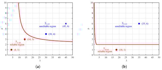
Figure 1. Reliable and unreliable regions for local and global asymptotic stability. (a) ${\mathsf{\Lambda }}_{\mathrm{L}\mathrm{A}\mathrm{S}}$ and ${\overline{\mathsf{\Lambda }}}_{\mathrm{L}\mathrm{A}\mathrm{S}}$ for local asymptotic stability; (b) ${\mathsf{\Lambda }}_{\mathrm{G}\mathrm{A}\mathrm{S}}$ and ${\overline{\mathsf{\Lambda }}}_{\mathrm{G}\mathrm{A}\mathrm{S}}$ for global asymptotic stability.

Similarly, we obtain a reliable region ${\mathsf{\Lambda }}_{\mathrm{GAS}}$ of $(\lambda ,b)$ by (15), and plot the corresponding boundary in Figure 1b. Based on Theorem 2, each pair of $(\lambda ,b)\in {\mathsf{\Lambda }}_{\mathrm{G}\mathrm{A}\mathrm{S}}$ guarantees the global asymptotic stability of fixed point $X_e$. It is obvious that the point $(\lambda ,b)=(18,1)$ is in ${\mathsf{\Lambda }}_{\mathrm{GAS}}$, over which all the solutions $X_t$ are oscillating around $X_e$ and eventually tends to $X_e$. Clearly, $(\lambda ,b)=(35,6)\in {\overline{\mathsf{\Lambda }}}_{\mathrm{G}\mathrm{A}\mathrm{S}}$, in the sense that all the solutions $X_t$ are divergent.

4.1. Locally Asymptotically Stable

We performed some numerical examples to analyze the dynamic behavior of solutions of system Equation (2). For $(\lambda ,b)=(4,1)\in {\mathsf{\Lambda }}_{\mathrm{L}\mathrm{A}\mathrm{S}}$, the fixed point $X_e=30$ is obtained by (8). Given an initial value $X_0=25$ in the vicinity of fixed point $X_e=30$, we obtain the dynamic behavior of $X_t$ with time series t, as shown in Figure 2a. We see that the solution $X_t$ is monotonically increasing to $X_e$ with the increment of t. Similarly, for $(\lambda ,b)=(14,3)\in {\mathsf{\Lambda }}_{\mathrm{L}\mathrm{A}\mathrm{S}}$, the corresponding fixed point of (8) is $X_e=14.1014$. Starting with an initial value $X_0=10$ near $X_e=14.1014$, the corresponding dynamic behavior of $X_t$ is illustrated in Figure 2b. It is interesting to see that solution $X_t$ is oscillating around $X_e$ and converging to $X_e$. The phenomena observed from Figure 2a,b coincide with our Theorem 1, in the sense that $X_e$ is locally asymptotically stable if $(\lambda ,b)\in {\mathsf{\Lambda }}_{\mathrm{L}\mathrm{A}\mathrm{S}}$.

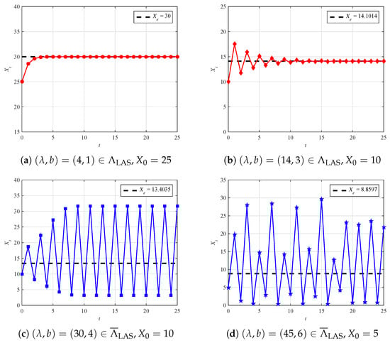
Figure 2. Locally asymptotically stable and unstable solution.

For comparison, for $(\lambda ,b)=(30,4)$ and $(45,6)$, both in the unreliable region ${\overline{\mathsf{\Lambda }}}_{\mathrm{LAS}}$, the fixed points are $X_e=13.4035$ and $8.8597$, respectively. Correspondingly, we also provide the dynamic behavior of $X_t$ in Figure 2c,d. From Figure 2c, it is easy to see that $X_t$ is periodic with Period 2 for $t\ge 9$. Figure 2d shows that $X_t$ is irregular for all t. These phenomena imply that $X_t$ is oscillatory and eventually divergent, in the sense that $X_e$ is unstable if $(\lambda ,b)\in {\overline{\mathsf{\Lambda }}}_{\mathrm{L}\mathrm{A}\mathrm{S}}$, no matter how close $X_0$ is to $X_e$.

4.2. Globally Asymptotically Stable

To verify our global asymptotic stability analysis results, we also offer some numerical examples to analyze the dynamic behavior of solutions $X_t$. For a given pair of $(\lambda ,b)=(18,1)\in {\mathsf{\Lambda }}_{\mathrm{GAS}}$, we calculate the fixed point $X_e=170$ by (8). When the initial value is given by $X_0=165$ near $X_e=170$, we provide the dynamic behavior of $X_t$ with time series t in Figure 3a. For comparison, for $X_0=280$ far away from $X_e=170$, we also plot $X_t$ in Figure 3b.

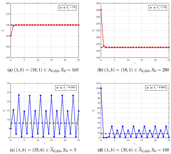
Figure 3. Globally asymptotically stable and unstable solution.

Figure 3a,b show that each solution $X_t$ converges monotonically to the fixed point $X_e$ for all $X_0$ with the increment of t. This verifies that our Theorem 2 is accurate, in the sense that $X_e$ is globally asymptotically stable if $(\lambda ,b)\in {\mathsf{\Lambda }}_{\mathrm{GAS}}$, regardless of whether the $X_0$ is close to $X_e$.

On the other hand, taking a pair of $(\lambda ,b)=(35,6)\in {\overline{\mathsf{\Lambda }}}_{\mathrm{GAS}}$, the fixed point is $X_e=8.0861$. For $X_0=5$ near $X_e=8.0861$ and $X_0=100$ far away from $X_e=8.0861$, we also offer the corresponding dynamic behavior of $X_t$, as depicted in Figure 3c,d, respectively. It is easy to show that all solutions $X_t$ oscillate infinitely about the fixed point $X_e$, but do not eventually converge to $X_e$. This occurrence makes the fixed point $X_e$ unstable. The reason is that Theorem 2 is not satisfied, i.e., $(\lambda ,b)\notin {\mathsf{\Lambda }}_{\mathrm{GAS}}$.

4.3. Time Delay

For the DLPG model with time delay T, it is represented by difference equation $X_t=\frac{\lambda X_{t-T}}{{\left(1+a{X}_{t-T}\right)}^b}$. We also present some numerical results to investigate the effect of time delay for asymptotic stability and species dynamics. The time delay is set to $T=5$.

For local asymptotic stability, the same parameters are set with Section 4.1. The corresponding dynamic behavior of $X_t$ with time series t are plotted in Figure 4. These phenomena observed from Figure 4 coincide with our Theorem 1. That is, if $(\lambda ,b)\in {\mathsf{\Lambda }}_{\mathrm{L}\mathrm{A}\mathrm{S}}$, $X_e$ is locally asymptotically stable. Otherwise, $X_e$ is unstable.

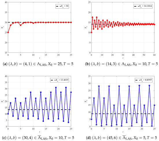
Figure 4. Locally asymptotically stable and unstable solution with time delay.

Similarly, for global asymptotic stability, the parameters are set the same as in Section 4.2. We obtain the corresponding results as shown in Figure 5. Clearly, if $(\lambda ,b)\in {\mathsf{\Lambda }}_{\mathrm{G}\mathrm{A}\mathrm{S}}$, $X_e$ is globally asymptotically stable, and vice versa. This is consistent with our Theorem 2.

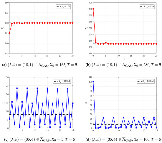
Figure 5. Globally asymptotically stable and unstable solution with time delay.

We note that, although the factor of time delay leads to slight perturbations for the curves of population dynamics, these variations do not affect the validity of our Theorems 1 and 2.

5. Conclusions

For a density dependent single-species population growth model, we proposed a simple method to explicitly and directly derive the analytic expressions of reliable regions for local and global asymptotic stability. Specifically, we explicitly represented first a reliable region ${\mathsf{\Lambda }}_{\mathrm{LAS}}$, over which the fixed point is locally asymptotically stable, by solving the fixed point equation and utilizing the asymptotic stability criterion. Then, we constructed two types of the auxiliary Liapunov function whose variation is decomposed into the product of two functions and is always negative at the non-equilibrium state. Finally, based on the Liapunov stability theorem, we obtained a closed-form expression of reliable region ${\mathsf{\Lambda }}_{\mathrm{GAS}}$, where the fixed point is globally asymptotically stable in the sense that all the solutions tend to it. Numerical results show that our analytic expressions of reliable regions were accurate for both local and global asymptotic stability.

In this paper, we mainly focused on the analytic expression of reliable region for global asymptotic stability by constructing relatively simple auxiliary Liapunov functions, such as the squared form of the difference and the logarithm. There are other more complicated forms of the Liapunov function. Moreover, the DLPG model can be applied to some specific species which are characterized by discrete reproductive cycles, such as zebrafish [18] and Pink salmon [19]. This paves the way to investigate the intricacies of population dynamics in the specific species. How to extend our method to them is an interesting issue for further investigation.

References

- Malthus, T.R. An Essay on the Principle of Population; 12th Media Services: Suwanee, GA, USA, 1798. [Google Scholar]
- Nicholson, A.J.; Bailey, V.A. The balance of animal populations. Part I. Proc. Zool. Soc. Lond. 1935, 105, 551–598. [Google Scholar] [CrossRef]
- May, R. Stability and Complexity in Model Ecosystems; Princeton University Press: Princeton, Hong Kong, 1973. [Google Scholar]
- Wang, L. Improvement of conditions for boundedness in a chemotaxis consumption system with density-dependent motility. Appl. Math. Lett. 2022, 125, 107724. [Google Scholar] [CrossRef]
- Hassell, M.P. Density dependence in single-species population. J. Anim. Ecol. 1975, 44, 283–295. [Google Scholar] [CrossRef]
- Elaydi, S. Discrete Chaos: With Applications in Science and Engineering, 2nd ed.; CRC Press: Boca Raton, FL, USA, 2008. [Google Scholar]
- Mathur, K.S.; Dhar, J. Stability and permanence of an eco-epidemiological SEIN model with impulsive biological control. Comp. Appl. Math. 2018, 37, 675–692. [Google Scholar] [CrossRef]
- Din, Q.; Elsadany, A.A.; Ibrahim, S. Bifurcation analysis and Chaos control in a second-order rational difference equation. Int. J. Nonlinear Sci. Numer. Simul. 2018, 19, 53–68. [Google Scholar] [CrossRef]
- Moaaz, O.; Chalishajar, D.; Bazighifan, O. Some qualitative behavior of solutions of general class of difference equations. Mathematics 2019, 7, 585. [Google Scholar] [CrossRef]
- Chen, C. Explicit solutions and stability properties of homogeneous polynomial dynamical systems. IEEE Trans. Autom. Control 2022, 68, 4962–4969. [Google Scholar] [CrossRef]
- Stone, L. The feasibility and stability of large complex biological networks: A random matrix approach. Sci. Rep. 2018, 8, 8246. [Google Scholar] [CrossRef] [PubMed]
- Wu, J.W.; Brown, D.P. Global asymptotic stability in discrete systems. J. Math. Anal. Appl. 1989, 140, 224–227. [Google Scholar] [CrossRef]
- Wörz-Busekros, A. Global stability in ecological systems with continuous time delay. SIAM J. Appl. Math. 1978, 35, 123–134. [Google Scholar] [CrossRef]
- Liz, E.; Buedo-Fernández, S. A new formula to get sharp global stability criteria for one-dimensional discrete-time models. Qual. Theory Dyn. Syst. 2019, 18, 813–824. [Google Scholar] [CrossRef]
- Hoang, M.T.; Egbelowo, O.F. On the global asymptotic stability of a hepatitis B epidemic model and its solutions by nonstandard numerical schemes. Bol. Soc. Mat. Mex. 2020, 26, 1113–1134. [Google Scholar] [CrossRef]
- Hoang, M.T. Global asymptotic stability of a general fractional-order single-species model. Bol. Soc. Mat. Mex. 2022, 28, 2. [Google Scholar] [CrossRef]
- Elaydi, S. An Introduction to Difference Equations, 3rd ed.; Springer Science & Business Media: Berlin/Heidelberg, Germany, 2005. [Google Scholar]
- Beaudouin, R.; Goussen, B.; Piccini, B.; Augustine, S.; Devillers, J.; Brion, F.; Péry, A.R. An individual-based model of zebrafish population dynamics accounting for energy dynamics. PLoS ONE 2015, 10, e0125841. [Google Scholar] [CrossRef] [PubMed]
- Krkošek, M.; Drake, J.M. On signals of phase transitions in salmon population dynamics. Proc. R. Soc. Biol. Sci. 2014, 281, 20133221. [Google Scholar] [CrossRef] [PubMed]
Disclaimer/Publisher’s Note: The statements, opinions and data contained in all publications are solely those of the individual author(s) and contributor(s) and not of MDPI and/or the editor(s). MDPI and/or the editor(s) disclaim responsibility for any injury to people or property resulting from any ideas, methods, instructions or products referred to in the content. |
© 2023 by the authors. Licensee MDPI, Basel, Switzerland. This article is an open access article distributed under the terms and conditions of the Creative Commons Attribution (CC BY) license (https://creativecommons.org/licenses/by/4.0/).