Minimum Residual Sum of Squares Estimation Method for High-Dimensional Partial Correlation Coefficient

Abstract

The partial correlation coefficient (Pcor) is a vital statistical tool employed across various scientific domains to decipher intricate relationships and reveal inherent mechanisms. However, existing methods for estimating Pcor often overlook its accurate calculation. In response, this paper introduces a minimum residual sum of squares Pcor estimation method (MRSS), a high-precision approach tailored for high-dimensional scenarios. Notably, the MRSS algorithm reduces the estimation bias encountered with positive Pcor. Through simulations on high-dimensional data, encompassing both sparse and non-sparse conditions, MRSS consistently mitigates the arithmetic bias for positive Pcors, surpassing other algorithms discussed. For instance, for large sample sizes ($n\ge 100$) with Pcor > 0, the MRSS algorithm reduces the MSE and RMSE by about 30–70% compared to other algorithms. The robustness and stability of the MRSS algorithm is demonstrated by the sensitivity analysis with variance and sparsity parameters. Stocks data in China’s A-share market are employed to showcase the MRSS methodology’s practicality.

1. Introduction

The partial correlation coefficient (Pcor) measures the correlation between two random variables, X and Y, after accounting for the effects of controlling variables Z, denoted by ${\rho }_{XY|Z}$. The Pcor essentially quantifies the unique relationship between X and Y, after removing the correlations between X and Z, and between Y and Z [1]. This correlation coefficient provides a more thorough comprehension of the connection between variables, untainted by the influence of confounding factors. Unlike the Pearson correlation coefficient, which only captures the direct correlation between random variables, the Pcor enables the identification of whether correlations stem from intermediary variables. This distinction enhances the precision and validity of statistical analyses.

The Pcor is a fundamental statistical tool for investigating intricate relationships and gaining a more profound comprehension of the underlying mechanisms in a variety of scientific fields, such as psychology, biology, economics, and social sciences. When examining genetic markers and illness outcomes, biologists used the Pcor to identify correlations while accounting for potential confounding factors [2,3,4]. Marrelec et al. utilised the partial correlation matrix to explore large-scale functional brain networks through functional MRI [5]. In the field of economics, Pcor assists in comprehending complex connections, including the interplay between interest rates and inflation, while considering other variables’ influence [6]. The financial industry also employs Pcor to interpret connections and relationships between stocks in the financial markets [7,8]. For example, Michis proposed a wavelet procedure for estimating Pcor between stock market returns over different time scales and implemented it for portfolio diversification [9]. Using partial correlations within a complex network framework, Singh et al. examined the degree of globalisation and regionalisation of stock market linkages and how these linkages vary across different economic or market cycles [10]. Meanwhile, the employment of the Gaussian graphical model (GGM) technique in psychology has recently gained popularity for defining the relationships between observed variables. This technique employs Pcors to represent pairwise interdependencies, controlling the influence of all other variables [11,12,13]. In the field of geography, a correlation analysis based on the Pcor of the fractal dimension of the variations of HZD components is implemented to study the geomagnetic field component variations in Russian [14].

Several methodologies have been proposed over the years to estimate the Pcor in statistical analyses. For instance, Peng et al. introduced a Pcor estimation technique that relies on the sparsity property of the partial correlation matrix and utilises sparse regression methods [3]. Khare et al. suggested a high-dimensional graphical model selection approach based on the use of pseudolikelihood [15]. Kim provided an R package “ppcor” for a fast calculation to semi-Pcor [16]. Huang et al. introduced the kernel partial correlation coefficient as a measure of the conditional dependence between two random variables in various topological spaces [17]. Van Aert and Goos focused on calculating the sampling variance of Pcor [18]. Hu and Qiu proposed a statistical inference procedure for Pcor under the high-dimensional nonparanormal model [19]. However, these methods mainly centre around determining whether or not the partial correlation coefficient is zero, without adequate regard for the precision of the Pcor calculation and the algorithm’s efficacy. We analysed multiple high-dimensional algorithms and discovered notable Pcor estimation biases, particularly for positive Pcor. Even with larger sample sizes, these biases persisted. Motivated by these findings, our primary goal is to put forward a Pcor estimation algorithm to increase the precision of the Pcor estimation algorithm and diminish the estimation bias for positive Pcor values.

This paper reviews current methods for estimating Pcor in high-dimensional data. We introduce a novel minimum residual sum of squares (MRSS) Pcor estimation method under high-dimensional conditions, aiming to mitigate the estimation bias for positive Pcor. The algorithm’s effectiveness is validated through simulation studies under sparse and non-sparse conditions and real data analysis on stock markets.

The sections are structured as follows: Section 2 outlines definitions and corresponding formulae for calculating Pcor, and examines common algorithms for estimating Pcor. Section 3 presents our Minimum Residual Sum of Squares Pcor estimation, designed to mitigate estimation bias for positive Pcor. In Section 4, we demonstrate the effectiveness of our proposed algorithm through simulation studies on high-dimensional data under both sparse and non-sparse conditions. Section 5 provides an analysis of real data related to stock markets, while Section 6 contains the conclusion.

2. Estimation for Partial Correlation Coefficient

2.1. Definition of Pcor

The classical definition of the partial correlation coefficient is defined by the correlation coefficient between the regression residuals from the linear models of two variables with the controlling variable, respectively. Let X and Y be two random variables, and $Z=[Z_1, Z_2, \cdots , Z_p]$ be p-dimensional controlling variables. Consider the linear regression models of X and Y, respectively, with the controlling variable Z,

$$\begin{array}{cc}\hfill X& ={\alpha }_0+{\sum }_{i=1}^p{\alpha }_i{Z}_i+\epsilon , \hfill \\ \hfill Y& ={\beta }_0+{\sum }_{i=1}^p{\beta }_i{Z}_i+\zeta , \hfill \end{array}$$

where $\epsilon$ and $\zeta$ are error terms. The partial correlation coefficient between X and Y is conditional on Z, denoted by ${\rho }_{XY|Z}$, and defined by the correlation coefficient between the regression residuals $\epsilon$ and $\zeta$, as follows  

$${\rho }_{XY|Z}=cor(\epsilon , \zeta )=\frac{cov(\epsilon , \zeta )}{\sqrt{var\left(\epsilon \right)}\sqrt{var\left(\zeta \right)}}.$$

(1)

where $cor(., .)$ is the correlation coefficient of two random variables; $cov(., .)$ is the covariance of two random variables; $var(.)$ is the variance of a random variable. Let the sample size be n. In conventional low-dimensional cases ($p<n$), the ordinary least squares (OLS) is used to compute the residuals $\epsilon$ and $\zeta$. Subsequently, the Pcor is computed from the correlation coefficient of residuals. However, the OLS method is not practical for high-dimensional cases ($p>n$). Regularisation methods are introduced to deal with such cases later.

2.2. Calculation Formulae of Pcor

2.2.1. Based on Concentration Matrix

The concentration matrix can also be used to calculate Pcor. Let $U_1=[X, Y]$, $U_2=Z$$=[Z_1, \cdots , Z_p]$, $U=[U_1, U_2]=[X, Y, Z]$ and $\mathsf{\Sigma }=cov\left(U\right)$ be the covariance matrix. When assuming that $\mathsf{\Sigma }$ is a non-singular matrix, the concentration matrix is denoted as $\mathsf{\Omega }={\left({\omega }^{ij}\right)}_{i, j=1}^{p+2}={\mathsf{\Sigma }}^{-1}$. Consider the following linear regression,

$$U_1=U_{2}b+e,$$

where $b=(b_1, b_2)$ is the regression coefficient and $e=(e_1, e_2)$ is the regression error. We have

$$\widehat{e}=({\widehat{e}}_1, {\widehat{e}}_2)=U_1-U_2\widehat{b}=U_1-{\widehat{U}}_1,$$

where $\widehat{b}$ is the estimator of b and ${\widehat{U}}_1$ is the estimator of $U_1$. The regression residual $\widehat{e}\sim N(0, V)$ is independent of ${\widehat{U}}_1$. The covariance matrix of $\widehat{e}$ can be computed by

$$\begin{array}{cc}\hfill cov\left(\widehat{e}\right)& =cov\left(U_1\right)+cov\left({\widehat{U}}_1\right)-2cov(U_1, {\widehat{U}}_1)\hfill \\ \hfill & ={\mathsf{\Sigma }}_{11}+{\mathsf{\Sigma }}_{12}{\mathsf{\Sigma }}_{22}^{-1}{\mathsf{\Sigma }}_{22}{\mathsf{\Sigma }}_{22}^{-1}{\mathsf{\Sigma }}_{21}-2{\mathsf{\Sigma }}_{12}{\mathsf{\Sigma }}_{22}^{-1}{\mathsf{\Sigma }}_{21}\hfill \\ \hfill & ={\mathsf{\Sigma }}_{11}-{\mathsf{\Sigma }}_{12}{\mathsf{\Sigma }}_{22}^{-1}{\mathsf{\Sigma }}_{21}={\mathsf{\Omega }}_{11}^{-1}.\hfill \end{array}$$

According to the definition in Equation (1) and ${\mathsf{\Omega }}_{11}^{-1}=\frac{1}{{\omega }^{11}{\omega }^{22}-{\omega }^{12}{\omega }^{21}}\left[\begin{array}{cc}{\omega }^{22}& -{\omega }^{12}\\ -{\omega }^{21}& {\omega }^{11}\end{array}\right],$ the partial correlation coefficient can be computed by

$${\rho }_{XY|Z}=cor({\widehat{e}}_1, {\widehat{e}}_2)=\frac{cov({\widehat{e}}_1, {\widehat{e}}_2)}{\sqrt{var\left({\widehat{e}}_1\right)}\sqrt{var\left({\widehat{e}}_2\right)}}=-\frac{{\omega }^{12}}{\sqrt{{\omega }^{11}}\sqrt{{\omega }^{22}}}.$$

(2)

2.2.2. Based on Additional Regression Models

Additional linear regression models are introduced to calculate the Pcor. Consider new linear regression models of X with $[Y, Z]$ and Y with $[X, Z]$, respectively,

$$\begin{array}{cc}\hfill X& ={\lambda }_{0}Y+{\sum }_{i=1}^p{\lambda }_i{Z}_i+\eta , \hfill \end{array}$$

(3)

$$\begin{array}{cc}\hfill Y& ={\gamma }_{0}X+{\sum }_{i=1}^p{\gamma }_i{Z}_i+\tau , \hfill \end{array}$$

(4)

where $\eta$ and $\tau$ are regression error terms. Peng et al. [3] established the correlation between the aforementioned regression coefficients and Pcor, while verifying that formulas ${\lambda }_0={\rho }_{XY|Z}\sqrt{\frac{{\omega }^{22}}{{\omega }^{11}}}, {\gamma }_0={\rho }_{XY|Z}\sqrt{\frac{{\omega }^{11}}{{\omega }^{22}}}$, $var\left(\eta \right)=\frac{1}{{\omega }^{11}}$ and $var\left(\tau \right)=\frac{1}{{\omega }^{22}}$ hold. Then, we derive ${\lambda }_0{\gamma }_0={\rho }_{XY|Z}^2$. Thus, the partial correlation coefficient between X and Y can be calculated by the formula below,

$$\begin{array}{cc}\hfill {\rho }_{XY|Z}& ={\lambda }_0\sqrt{var\left(\tau \right)/var\left(\eta \right)}, \hfill \end{array}$$

(5)

$$\begin{array}{cc}\hfill & =sign\left({\lambda }_0\right)\sqrt{{\lambda }_0{\gamma }_0}, \hfill \end{array}$$

(6)

where $sign(·)$ is the sign function.

Consider linear regression models of Y with $[1, Z]$ and Y with $[1, X, Z]$, respectively,

$$\begin{array}{cc}\hfill Y& ={\beta }_0+{\sum }_{i=1}^p{\beta }_i{Z}_i+\zeta , \hfill \\ \hfill Y& ={\gamma }_{-1}+{\gamma }_{0}X+{\sum }_{i=1}^p{\gamma }_i{Z}_i+\tau , \hfill \end{array}$$

where $\zeta$ and $\tau$ are error terms. The partial correlation coefficient can also be calculated as follows [20]

$${\rho }_{XY|Z}=sign\left({\gamma }_0\right)\sqrt{\frac{var\left(\zeta \right)-var\left(\tau \right)}{var\left(\zeta \right)}}.$$

(7)

Here, we present five distinct formulae, (1), (2), (5), (6), and (7), for calculating Pcor based on diverse regression models. Specific algorithms applicable to high-dimensional scenarios will be presented in the following section.

2.3. Regularisation Regression for High-Dimensional Cases

Suppose we have centralised samples ${\{x_j, y_j, z_{j1}, \dots , z_{jp}\}}_{j=1}^n$ i.i.d. observed from $[X, Y, Z]$ with $Z=[Z_1, \dots , Z_p]$. Let $\mathbf{X}={[x_1, \dots , x_n]}^T$, $\mathbf{Y}={[y_1, \cdots , y_n]}^T$ and $\mathbf{Z}=[{\mathbf{Z}}_1, \dots , {\mathbf{Z}}_p]=$${\left(z_{ji}\right)}_{n\times p}$. We consider matrix-type linear regression models as follows,

$$\begin{array}{cc}\hfill \mathbf{X}& ={\sum }_{i=1}^p{\alpha }_i{\mathbf{Z}}_i+\epsilon , \hfill \end{array}$$

(8)

$$\begin{array}{cc}\hfill \mathbf{Y}& ={\sum }_{i=1}^p{\beta }_i{\mathbf{Z}}_i+\zeta , \hfill \end{array}$$

(9)

where $\epsilon ={[{\epsilon }_1, \dots , {\epsilon }_n]}^T$ and $\zeta ={[{\zeta }_1, \dots , {\zeta }_n]}^T$ are error terms. If we estimate regression coefficients $\widehat{\alpha }={[{\widehat{\alpha }}_1, \dots , {\widehat{\alpha }}_p]}^T$ and $\widehat{\beta }={[{\widehat{\beta }}_1, \dots , {\widehat{\beta }}_p]}^T$, then we can calculate the estimated residuals $\widehat{\epsilon }=\mathbf{X}-\widehat{\mathbf{X}}$ and $\widehat{\zeta }=\mathbf{Y}-\widehat{\mathbf{Y}}$, with $\widehat{\mathbf{X}}=\mathbf{Z}\widehat{\alpha }={\sum }_{i=1}^p{\widehat{\alpha }}_i{\mathbf{Z}}_i$ and $\widehat{\mathbf{Y}}=\mathbf{Z}\widehat{\beta }={\sum }_{i=1}^p{\widehat{\beta }}_i{\mathbf{Z}}_i$. According to the definition of Pcor, we can estimate the Pcor as follows

$$\widehat{\rho }=\frac{cov(\widehat{\epsilon }, \widehat{\zeta })}{\sqrt{var\left(\widehat{\epsilon }\right)var\left(\widehat{\zeta }\right)}},$$

(10)

where $cov(\widehat{\epsilon }, \widehat{\zeta })={\sum }_{j=1}^n({\widehat{\epsilon }}_j-\overline{\epsilon })({\widehat{\zeta }}_j-\overline{\zeta })$, $var\left(\widehat{\epsilon }\right)={\sum }_{j=1}^n{({\widehat{\epsilon }}_j-\overline{\epsilon })}^2$ and $var\left(\widehat{\zeta }\right)={\sum }_{j=1}^n{({\widehat{\zeta }}_j-\overline{\zeta })}^2$ with $\overline{\epsilon }=\frac{1}{n}{\sum }_{j=1}^n{\widehat{\epsilon }}_j$, $\overline{\zeta }=\frac{1}{n}{\sum }_{j=1}^n{\widehat{\zeta }}_j$.

In high-dimensional ($p>n$) situations, the penalty function and regularisation regression methods can be introduced to estimate the regression coefficients for regression models. Regularisation regression methods address overfitting in statistical modelling by adding a penalty to the loss function, constraining the coefficient magnitudes. Let $p_{\lambda }\left(\beta \right)$ be the penalty function with a tuning parameter $\lambda$, for example, the regularisation estimate of model (8) is given by

$$\widehat{\alpha }=\underset{\alpha }{arg\; min}\frac{1}{n}{\left|\right|\mathbf{X}-\mathbf{Z}\alpha \left|\right|}^2+p_{\lambda }\left(\alpha \right),$$

where the penalty $p_{\lambda }\left(\alpha \right)$ could widely choose the Lasso penalty [21], the Ridge penalty [22], the SCAD penalty [23], the Elastic net [24], the Fused lasso [25], the MCP penalty [26], and other penalty functions. In this paper, the Lasso regularisation with penalty as $p_{\lambda }\left(\alpha \right)={\lambda \left|\right|\alpha \left|\right|}_1$ is implemented by the R-package “glmnet” [27], and the MCP with penalty as $p_{\lambda }\left(\alpha \right)=\frac{1}{t}{(t\lambda -\alpha )}_{+}$, $(t>1)$ is implemented by the R-package “ncvreg”.

2.4. Existing Pcor Estimation Algorithms

To investigate high-dimensional Pcor estimation methods, we present some existing methods that are suitable for both sparse and non-sparse conditions. Combining the advantages and disadvantages of these methods, we propose a new high-dimensional Pcor estimation method: MRSS—minimum residual sum of squares partial correlation coefficient estimation algorithm.

2.4.1. Res Algorithm

The Res algorithm is primarily defined by the Pcor definition. This algorithm is implemented as follows. First, we use the regularisation regression (Lasso and MCP) on linear models (8) and (9) to obtain the estimated regression coefficients $\widehat{\alpha }$ and $\widehat{\beta }$; then calculate estimated residuals $\widehat{\epsilon }=\mathbf{X}-\widehat{\mathbf{X}}$ and $\widehat{\zeta }=\mathbf{Y}-\widehat{\mathbf{Y}}$, with $\widehat{\mathbf{X}}=\mathbf{Z}\widehat{\alpha }$ and $\widehat{\mathbf{Y}}=\mathbf{Z}\widehat{\beta }$; at last, estimate Pcor ${\widehat{\rho }}_{res}$ by formula (10).

2.4.2. Reg2 Algorithm

The Reg2 algorithm can more effectively remove the influence of Z in X and Y using the new regressions below. Consider new linear regression models as follows

$$\begin{array}{cc}\hfill \mathbf{X}& =a_1\widehat{\mathbf{X}}+a_2\widehat{\mathbf{Y}}+{\eta }_1, \hfill \end{array}$$

(11)

$$\begin{array}{cc}\hfill \mathbf{Y}& =b_1\widehat{\mathbf{X}}+b_2\widehat{\mathbf{Y}}+{\tau }_1, \hfill \end{array}$$

(12)

where ${\eta }_1$ and ${\tau }_1$ are error terms, the estimators $\widehat{\mathbf{X}}={\sum }_{i=1}^p{\widehat{\alpha }}_i{\mathbf{Z}}_i$ and $\widehat{\mathbf{Y}}={\sum }_{i=1}^p{\widehat{\beta }}_i{\mathbf{Z}}_i$ are estimated by the Lasso or MCP regularisation regressions of models (8) and (9). Then, we implement the ordinary least squares (OLS) on models (11) and (12), and denote new estimators of $\mathbf{X}$ and $\mathbf{Y}$ by ${\widehat{\mathbf{X}}}_{Reg2}$ and ${\widehat{\mathbf{Y}}}_{Reg2}$. Computing new residuals ${\widehat{\eta }}_1=\mathbf{X}-{\widehat{\mathbf{X}}}_{Reg2}$ and ${\widehat{\tau }}_1=\mathbf{Y}-{\widehat{\mathbf{Y}}}_{Reg2}$, we finally estimate Pcor by the Reg2 algorithm as ${\widehat{\rho }}_{reg2}=cor({\widehat{\eta }}_1, {\widehat{\tau }}_1)$.

2.4.3. Coef and Var Algorithm

The Coef and Var algorithm is generated through the introduction of novel regression coefficients based on the Pcor definition formula (5) and (6). Consider linear regression models as follows

$$\begin{array}{cc}\hfill \mathbf{X}& ={\lambda }_0\mathbf{Y}+{\sum }_{i=1}^p{\lambda }_i{\mathbf{Z}}_i+{\eta }_2, \hfill \end{array}$$

(13)

$$\begin{array}{cc}\hfill \mathbf{Y}& ={\gamma }_0\mathbf{X}+{\sum }_{i=1}^p{\gamma }_i{\mathbf{Z}}_i+{\tau }_2, \hfill \end{array}$$

(14)

where ${\eta }_2$ and ${\tau }_2$ are error terms. Then, we implement MCP regularisation on these models (13) and (14) and obtain estimated first-term regression coefficients ${\widehat{\lambda }}_0$, ${\widehat{\gamma }}_0$ and the estimated variance $var\left({\widehat{\eta }}_2\right)$, $var\left({\widehat{\tau }}_2\right)$. Finally, we can obtain the Pcor estimate by Coef algorithm as ${\widehat{\rho }}_{coef}=sign\left({\widehat{\lambda }}_0\right)\sqrt{{\widehat{\lambda }}_0{\widehat{\gamma }}_0}$ and the Pcor estimate by Var algorithm as ${\widehat{\rho }}_{var}={\widehat{\lambda }}_0\sqrt{var\left({\widehat{\tau }}_2\right)/var\left({\widehat{\eta }}_2\right)}$.

2.4.4. RSS2 Algorithm

The RSS2 algorithm is given by the residual sum of squares in formula (7). First, we implement the MCP regularisation on model (9): $\mathbf{Y}=\mathbf{Z}\beta +\zeta$ and estimate the residual $\widehat{\zeta }$ and the residual sum of squares (RSS) $R_1=\left|\right|\widehat{\zeta }{\left|\right|}_2^2$. Similarly, we implement the MCP regularisation on model (14): $\mathbf{Y}={\gamma }_0\mathbf{X}+{\sum }_{i=1}^p{\gamma }_i{\mathbf{Z}}_i+\tau$ and estimate the first-term regression coefficient ${\widehat{\gamma }}_0$, the residual $\widehat{\tau }$, and the RSS $R_2=\left|\right|\widehat{\tau }{\left|\right|}_2^2$. Then, we obtain the Pcor estimate ${\widehat{\rho }}_Y=sign\left({\widehat{\gamma }}_0\right)\sqrt{max(0, R_1-R_2)/R_1}$. Switch the position of $\mathbf{X}$ and $\mathbf{Y}$ similarly as the above steps. Then, we implement the MCP regularisation on model (8): $\mathbf{X}=\mathbf{Z}\alpha +\epsilon$ and model (13): $\mathbf{X}={\lambda }_0\mathbf{Y}+{\sum }_{i=1}^p{\lambda }_i{\mathbf{Z}}_i+\eta$ and obtain the RSS $R_3=\left|\right|\widehat{\epsilon }{\left|\right|}_2^2$, $R_4=\left|\right|\widehat{\eta }{\left|\right|}_2^2$ and the estimated first-term coefficient ${\widehat{\lambda }}_0$. We obtain another Pcor estimate ${\widehat{\rho }}_X=sign\left({\widehat{\lambda }}_0\right)\sqrt{max(0, R_3-R_4)/R_3}$. Finally, we have the estimate Pcor by RSS2 algorithm as ${\widehat{\rho }}_{rss2}=({\widehat{\rho }}_X+{\widehat{\rho }}_Y)/2$.

3. Minimum Residual Sum of Squares Pcor Estimation Algorithm

3.1. Motivation

From the comprehensive simulations in this paper, it is evident that the Pcor estimation methods discussed exhibit significant bias. This bias becomes more pronounced as the true Pcor increases, especially when the Pcor is positive. Therefore, further research is necessary to address this estimation bias in positive Pcor scenarios. While each algorithm has its merits, the Reg2 algorithm performs notably well when Pcor is below approximately $0.5$. In contrast, the Coef and Var algorithm stands out with minimal bias when Pcor exceeds roughly $0.5$. Our goal is to develop a method that synergises the strengths of both the Reg2 and Var algorithms.

The models introduced in the Reg2 algorithm, (11) and (12), can be represented as,

$$\begin{array}{cc}\hfill \mathbf{X}& =a_1\widehat{\mathbf{X}}+a_2{\sum }_{i=1}^p{\widehat{\beta }}_i{\mathbf{Z}}_i+{\eta }_1, \hfill \end{array}$$

(15)

$$\begin{array}{cc}\hfill \mathbf{Y}& =b_2\widehat{\mathbf{Y}}+b_1{\sum }_{i=1}^p{\widehat{\alpha }}_i{\mathbf{Z}}_i+{\tau }_1, \hfill \end{array}$$

(16)

When compared to models (13) and (14) from the Coef and Var algorithm, it is evident that the residuals ${\eta }_1$ and ${\eta }_2$ share commonalities. Both provide insights into the information in X after the exclusion of Y and Z effects in some sense. Similarly, ${\tau }_1$ and ${\tau }_2$ capture the essence of Y after removing for X and Z influences. If we choose a ${\eta }_i$ and ${\tau }_i$ with a smaller residual sum of squares, then this will lead to a better estimation for the corresponding regression models. A reduced residual sum of squares in the corresponding regression models signifies enhanced precision in eliminating controlling variables effects, leading to a more accurate Pcor estimator. Guided by the objective of minimising the residual sum of squares, we introduce a novel algorithm for high-dimensional Pcor estimation in the subsequent subsection.

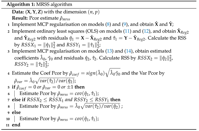
3.2. MRSS Algorithm and Its Implementation

We propose a novel Minimum Residual Sum of Squares partial correlation coefficient estimation algorithm, denoted by MRSS. This algorithm aims to diminish the estimation bias for positive Pcor values under high-dimensional situations. Our MRSS algorithm amalgamates the strengths of the Reg2, Coef, and Var algorithms, effectively curtailing bias in Pcor estimation.

Define $RSSX=\parallel {\eta }_k{\parallel }_2^2$ and $RSSY=\parallel {\tau }_k{\parallel }_2^2$ as the residual sum of squares of X after removing the effects of X and Z, and the residual sum of squares of Y after removing the effects of X and Z, respectively. The tuning parameter k is chosen by minimising the sum of squares of the residuals, so as to remove more associated effects and ensure a more efficient Pcor estimator. For $k=1$, the pair $({\eta }_1, {\tau }_1)$ represents the residuals from the Reg2 algorithm’ models (11) and (12). For $k=2$, $({\eta }_2, {\tau }_2)$ corresponds to the residuals from the Coef and Var algorithms’ models (13) and (14). Then, the residuals estimated by the MRSS algorithm satisfy the minimum residual sum of squares of both X and Y for a more efficient Pcor estimator as follows

$$\begin{array}{cc}\hfill {\eta }_{mrss}& =\underset{k=1, 2}{arg\; min}RSSX=\underset{k=1, 2}{arg\; min}{\parallel {\eta }_k\parallel }_2^2, \hfill \\ \hfill {\tau }_{mrss}& =\underset{k=1, 2}{arg\; min}RSSY=\underset{k=1, 2}{arg\; min}{\parallel {\tau }_k\parallel }_2^2.\hfill \end{array}$$

(17)

The Pcor estimated by MRSS is then given by

$${\rho }_{mrss}=cor({\eta }_{mrss}, {\tau }_{mrss})I_{k=1}+{\lambda }_0\sqrt{var\left({\tau }_{mrss}\right)/var\left({\eta }_{mrss}\right)}{I}_{k=2}$$

(18)

where I is the indicator function and ${\lambda }_0$ is the primary regression coefficient in model (13). If $k=1$, then ${\rho }_{mrss}$ is estimated following the idea of Reg2 algorithm; if $k=2$, then ${\rho }_{mrss}$ is estimated following the idea of the Coef and Var algorithm. If the two k estimates in (17) differ, the more stable Reg2 algorithm is preferred, setting $k=1$ in (18). Given that MRSS integrates two existing algorithms, its convergence should align with their rates.

During the implementation of the MRSS algorithm (Algorithm 1), the Coef and Var algorithm often misestimates Pcor as 0 or $\pm 1$ when the true Pcor is close to 0 or $\pm 1$, affecting the algorithms’ precision. To address this, we incorporate a discriminative condition in the MRSS pseudo-code. If the estimated Pcor ${\widehat{\rho }}_{coef}$ or ${\widehat{\rho }}_{var}$ is zero or $\pm 1$, the Coef and Var algorithm is deemed unreliable, and the Reg2 algorithm’s estimate is adopted.

The proposed MRSS algorithm selects the most suitable residuals by minimising RSS and removing the impact of control variables to optimise the estimation of residuals in the regression model. As such, the estimated Pcor generated by the MRSS algorithm combines the advantages of both algorithms, resulting in a more accurate estimate. Notably, our MRSS algorithm effectively addresses the Pcor estimation bias in cases where $\mathrm{Pcor}\ge 0$. For instance, when the Coef and Var algorithms estimate Pcor as 0 for true Pcor near 0, the MRSS algorithm utilises the minimum RSS principle to select the Reg2 algorithm, which performs better in the vicinity of $\mathrm{Pcor}=0$, and thereby efficiently avoids such misestimations. Around Pcor $=0.5$, the MRSS algorithm employs the minimum RSS principle to determine the more accurate method between Reg2 and Var for exact selection. This selection conforms to the minimum RSS principle, where the regression model and accompanying residuals are selected to provide optimal estimation accuracy, leading to a more precise Pcor estimate. When Pcor lies close to 1, the Reg2 algorithm’s estimates are typically lower with a high RSSs. Thereafter, the MRSS method selects the Var algorithm with small RSSs, which performs better based on the minimum RSS principle. In essence, the MRSS method amalgamates the merits of the Reg2 and Var algorithms. By reducing the sum of squares of the residuals, MRSS can choose the algorithm with a smaller estimation error for $\mathrm{Pcor}\ge 0$, which allows for the proficient regulation of the estimation bias of Pcor.

4. Simulation

4.1. Data Generation

To study the estimation efficiency of Pcor estimation algorithms under high-dimensional conditions, we generate n centralised samples ${\{x_j, y_j, z_{j1}, \dots , z_{jp}\}}_{j=1}^n$ i.i.d from $[X, Y, Z]$ with $Z=[Z_1, \dots , Z_p]$. Let $\mathbf{X}={[x_1, \dots , x_n]}^T$, $\mathbf{Y}={[y_1, \dots , y_n]}^T$ and $\mathbf{Z}=[{\mathbf{Z}}_1, \dots , {\mathbf{Z}}_p]={\left(z_{ji}\right)}_{n\times p}$. Initially, we produce n controlling samples ${\left\{{\mathbf{Z}}_i\right\}}_{i=1}^p$ independently and identically by

$${\mathbf{Z}}_i=0.5\mathbf{u}+{\mathbf{e}}_i$$

where $\mathbf{u}={[u_1, \dots , u_n]}^T$ and ${\mathbf{e}}_i={[e_{1i}, \dots , e_{ni}]}^T$ with $u_j$ and $e_{ji}$ generated independently from the normal distribution $N(0, {\sigma }^2)$ with variance ${\sigma }^2$ for $i=1, \dots , p$. The samples $\mathbf{X}$ and $\mathbf{Y}$ are then generated by

$$\mathbf{X}=\sum _{i=1}^p{\alpha }_i{\mathbf{Z}}_i+\epsilon , \mathrm{and}\mathbf{Y}=\sum _{i=1}^p{\beta }_i{\mathbf{Z}}_i+\zeta ,$$

where $\epsilon ={[{\epsilon }_1, \dots , {\epsilon }_n]}^T$ and $\zeta ={[{\zeta }_1, \dots , {\zeta }_n]}^T$ with ${\zeta }_j=\frac{\omega {\epsilon }_j+{\eta }_j}{\sqrt{1+{\omega }^2}}$ and ${\epsilon }_j$, ${\eta }_j$ drawn i.i.d. from $N(0, {\sigma }^2)$. The Pearson correlation of $\epsilon$ and $\zeta$ gives the partial correlation coefficient Pcor ${\rho }_{XY|Z}=\frac{\omega }{\sqrt{1-{\omega }^2}}$. Notably, there is a one-to-one mapping between the true Pcor and the $\omega$ parameter.

Since our MRSS algorithm and the Reg2 algorithm perform essentially the same for $\mathrm{Pcor}<0$, our simulation focuses on real Pcor values in the range $[0, 1]$, an interval prone to significant biases with existing methods. Let the true partial correlation coefficient vary as $Pcor=0, 0.05, 0.1, \dots , 0.95$ with the sample size $n=50, 100, \dots , 400$, the controlling variable size $p=200, 500, 1000$, $2000, 4000$ and the normal distribution variance ${\sigma }^2=1, 10, 40$. For each $n, p$ combination, we estimate the partial correlation coefficient for 200 replications using the aforementioned estimation algorithms. We use the software R (4.3.1) for our simulation.

Recognising that both sparse and non-sparse conditions are prevalent in real-world applications [3,28], we present examples under both conditions. To ensure comparability between the examples, the initial l coefficients of $\alpha$ and $\beta$ are fixed under both conditions, where we select the high-correlated numbers of controlling variables as $l=6, 10, 14$. For non-sparse examples, the coefficients of $\alpha$ and $\beta$ asymptotically converge to 0 at varying rates, with coefficients beyond the $(l+1)$-th starting at $0.05$, which is significantly smaller than the initial l coefficients.

• Example 1: under sparse conditions
  Let the coefficients $\alpha$ and $\beta$ be non-zero for the initial l elements and zero for the rest as follows
  $$\alpha =-\beta =(-0.1, -0.2, \dots , -\frac{l}{20}, 0.1, 0.2, \dots , \frac{l}{20}, 0, ..., 0).$$
• Example 2: under non-sparse conditions
  Let the coefficients $\alpha$ and $\beta$ be the same as Example 1 for the initial l elements with a convergence rate of $O(1/2^p)$ for the remaining elements as follows
  $$\alpha =-\beta =(-0.1, -0.2, \dots , \frac{l}{20}, \frac{r}{2^{l/2+1}}, \frac{r}{2^{l/2+2}}, \dots , \frac{r}{2^{p/2}}, -\frac{r}{2^{l/2+1}}, \dots , -\frac{r}{2^{p/2}}),$$

  where r is a tuning parameter to make the $(l+1)$-th element close to $0.05$.
• Example 3: under non-sparse conditions
  Let the coefficients $\alpha$ and $\beta$ be the same as Example 1 for the initial l elements with a convergence rate of $O(1/p)$ for the remaining elements as follows,
  $$\alpha =-\beta =(-0.1, -0.2, \dots , \frac{l}{20}, \frac{r}{l/2+1}, \frac{r}{l/2+2}, \dots , \frac{r}{p/2}, -\frac{r}{l/2+1}, \dots , -\frac{r}{p/2}),$$

  where r is a tuning parameter to make the $(l+1)$-th element close to $0.05$.
• Example 4: under non-sparse conditions
  Let the coefficients $\alpha$ and $\beta$ be the same as Example 1 for the initial l elements with a convergence rate of $O(1/\sqrt{p})$ for the remaining elements as follows,
  $$\alpha =-\beta =(-0.1, -0.2, \dots , \frac{l}{20}, \frac{r}{\sqrt{l/2+1}}, \frac{r}{\sqrt{l/2+2}}, \dots , \frac{r}{\sqrt{p/2}}, -\frac{r}{\sqrt{l/2+1}}, \dots , -\frac{r}{\sqrt{p/2}}),$$

  where r is a tuning parameter to make the $(l+1)$-th element close to $0.05$.

4.2. Simulation Results

4.2.1. By MSE and RMSE

We will assess the efficacy of the Pcor estimation algorithms using the mean square error (MSE) and root mean square error (RMSE) indices as follows. These evaluation indicators may indicate the performance of Pcor estimation algorithms from various perspectives.

$$MSE\left({\rho }_0\right)=\frac{1}{R}\sum _{i=1}^R{({\widehat{\rho }}_{\left(i\right)}-{\rho }_0)}^2, \mathrm{and}RMSE\left({\rho }_0\right)=\sqrt{\frac{1}{R}{\sum }_{i=1}^R{({\widehat{\rho }}_{\left(i\right)}-{\rho }_0)}^2},$$

where ${\rho }_0$ is the true Pcor, and ${\widehat{\rho }}_{\left(i\right)}$ is the estimated Pcor in the $\left(i\right)$-th replication of $R=200$ replications.

Table 1 displays the mean of MSE and RMSE ($\times {10}^2$) for the estimated Pcors of the true $\mathrm{Pcor}=0, 0.05$, $\dots , 0.95$ with $l=10$, ${\sigma }^2=1$, $n=50, 100, 200, 400$ and $p=200, 500, 1000, 2000, 4000$ across Examples 1–4 using various methods. Table A1 and Table A2, which consider the means of MSE and RMSE ($\times {10}^2$) for the estimated Pcors for high correlation controlling variables number $l=6, 14$, can be found in the Appendix.

Table 1. The mean of MSE ($\times {10}^2$) and RMSE ($\times {10}^2$) for estimated Pcors of real $\mathrm{Pcor}=0, 0.05, \dots , 0.95$ with $l=10$, ${\sigma }^2=1$, $n=50, 100, 200, 400$ and $p=200, 500, 1000, 2000, 4000$ in Examples 1–4.

		MSE ($\times {10}^2$)								RMSE ($\times {10}^2$)
Example 1		Lasso		MCP						Lasso		MCP
$\mathit{n}$	$\mathit{p}$	Res	Reg2	Res	Reg2	Coef	Var	RSS2	MRSS	Res	Reg2	Res	Reg2	Coef	Var	RSS2	MRSS
50	200	36.7	21.7	37.6	27.4	34.6	35.4	34.6	27.1	59.2	44.4	59.9	50.8	55.2	56.3	55.6	50.5
	500	46.8	29.6	47.2	36.0	34.4	35.3	36.4	35.5	66.9	51.9	67.2	58.2	54.9	56.0	57.3	57.5
	1000	51.4	33.0	50.7	39.3	34.1	34.8	36.6	38.8	70.2	54.8	69.7	60.8	54.3	55.3	57.5	60.3
100	500	22.1	11.7	15.2	9.5	24.2	21.5	14.0	7.7	45.9	32.4	38.1	29.9	47.9	46.0	35.5	27.3
	1000	29.6	16.1	22.4	13.9	32.5	30.0	22.6	13.4	53.1	37.8	46.1	36.1	54.5	53.5	45.2	35.4
	2000	36.1	19.7	29.6	18.4	35.0	34.3	29.4	18.2	58.8	41.7	53.2	41.5	56.1	56.3	51.1	41.3
200	500	6.6	3.1	1.7	1.5	2.4	2.6	1.8	0.7	25.1	17.3	12.8	12.1	12.7	13.3	11.5	7.6
	1000	9.6	5.2	2.5	2.2	3.8	4.3	2.4	0.9	30.2	22.1	15.6	14.5	16.4	17.1	13.1	8.9
	2000	13.0	7.9	3.6	3.1	6.0	6.6	3.3	1.4	35.3	27.0	18.6	17.3	21.0	21.5	15.3	10.5
400	1000	2.7	1.3	0.5	0.5	0.7	0.6	0.7	0.2	16.1	11.3	6.7	6.8	6.3	6.0	6.7	4.4
	2000	3.8	2.2	0.6	0.6	0.8	0.7	0.9	0.3	19.2	14.6	7.8	8.0	6.8	6.4	7.5	4.9
	4000	5.2	3.5	0.8	0.9	1.0	0.9	1.1	0.4	22.3	18.4	9.0	9.3	7.7	7.5	8.7	5.6
Example 2
50	200	37.0	21.8	38.3	28.1	34.7	35.8	34.9	27.9	59.4	44.4	60.4	51.3	55.3	56.7	56.0	51.2
	500	47.1	29.5	47.6	36.5	34.5	35.4	36.4	36.0	67.1	51.7	67.4	58.5	55.0	56.1	57.2	58.0
	1000	51.7	33.6	51.3	39.8	34.1	34.8	36.9	39.2	70.4	55.4	70.1	61.2	54.4	55.2	57.8	60.5
100	500	22.6	12.0	15.7	9.9	25.1	22.6	14.9	8.1	46.5	32.8	38.7	30.5	48.8	47.1	36.7	28.0
	1000	30.0	16.5	23.0	14.4	33.3	30.8	23.4	13.9	53.5	38.1	46.8	36.6	55.1	54.1	45.8	36.2
	2000	36.6	20.1	30.3	19.2	35.3	34.7	30.0	19.0	59.2	42.1	53.8	42.4	56.4	56.6	51.6	42.2
200	500	6.9	3.4	1.9	1.7	2.6	2.8	1.9	0.8	25.8	17.9	13.7	12.9	13.5	14.0	11.8	8.2
	1000	9.9	5.6	2.8	2.4	4.1	4.6	2.6	1.1	30.8	22.8	16.4	15.4	17.0	17.9	13.4	9.5
	2000	13.5	8.3	3.9	3.4	6.4	6.9	3.5	1.5	35.9	27.6	19.5	18.1	21.6	22.3	15.8	11.2
400	1000	2.9	1.5	0.6	0.6	0.7	0.6	0.7	0.3	16.8	12.1	7.5	7.5	6.7	6.4	6.9	4.9
	2000	4.1	2.5	0.8	0.8	0.9	0.8	0.9	0.4	19.9	15.4	8.6	8.8	7.3	7.0	7.8	5.5
	4000	5.5	3.9	1.0	1.1	1.1	1.0	1.2	0.5	23.0	19.3	9.8	10.3	8.3	8.1	9.1	6.3
Example 3
50	200	38.5	23.0	39.9	29.5	35.1	36.2	35.5	29.4	60.6	45.7	61.6	52.7	55.7	57.2	56.5	52.5
	500	48.7	30.6	49.2	37.9	34.8	35.7	37.1	37.3	68.3	52.7	68.5	59.6	55.4	56.5	58.0	59.0
	1000	53.4	34.5	53.0	41.4	34.5	35.4	37.4	40.9	71.5	56.0	71.2	62.4	54.9	56.1	58.4	61.9
100	500	24.4	13.3	17.8	11.5	27.9	25.5	17.3	10.1	48.3	34.6	41.2	32.8	51.3	50.0	39.6	31.1
	1000	31.9	17.5	25.2	16.1	34.6	33.1	26.5	15.8	55.2	39.3	49.0	38.8	56.2	55.9	48.6	38.5
	2000	38.8	21.5	32.4	20.7	36.0	35.8	31.7	20.6	61.0	43.6	55.6	44.1	57.1	57.6	53.0	44.0
200	500	8.3	4.4	2.8	2.6	3.6	3.9	2.5	1.3	28.1	20.3	16.5	15.8	17.1	17.7	14.0	11.1
	1000	11.6	6.9	4.0	3.5	5.5	6.2	3.3	1.7	33.3	25.2	19.5	18.3	21.1	22.1	16.0	12.8
	2000	15.4	9.7	5.4	4.7	8.3	8.9	4.6	2.3	38.3	29.8	22.6	21.1	26.2	26.8	18.8	14.6
400	1000	4.0	2.3	1.1	1.2	1.2	1.0	1.0	0.6	19.6	15.1	10.6	10.6	9.5	9.2	8.9	7.7
	2000	5.4	3.6	1.4	1.5	1.4	1.3	1.2	0.8	22.8	18.6	11.9	12.0	10.4	10.1	9.9	8.5
	4000	7.0	5.2	1.8	1.9	1.7	1.6	1.6	0.9	25.9	22.3	13.1	13.5	11.6	11.5	11.2	9.4
Example 4
50	200	41.7	25.4	43.6	32.8	36.3	37.6	37.2	32.6	63.1	48.1	64.4	55.6	57.2	58.7	58.3	55.4
	500	53.8	34.3	54.3	42.6	36.1	37.2	38.9	41.9	71.7	56.0	72.0	63.3	57.0	58.2	60.0	62.6
	1000	58.9	38.3	58.9	46.8	35.9	36.9	39.9	45.7	75.2	59.3	75.1	66.4	56.7	57.8	61.1	65.3
100	500	30.4	17.3	24.8	16.9	35.5	34.6	25.9	16.6	53.9	39.4	48.6	39.9	57.6	57.8	48.1	39.7
	1000	39.7	22.5	34.6	23.5	38.4	39.5	33.6	23.4	61.6	44.8	57.4	46.8	59.8	61.1	54.5	46.8
	2000	48.0	27.1	43.2	29.7	39.5	40.8	37.0	29.5	67.8	49.3	64.3	52.9	60.9	62.1	57.9	52.7
200	500	12.9	8.1	6.8	6.3	8.7	9.3	5.5	4.5	35.1	27.4	25.5	24.4	28.7	29.8	22.1	21.1
	1000	18.5	12.4	9.8	8.8	13.9	15.0	8.2	6.7	42.1	33.7	30.6	28.9	36.5	38.0	26.9	25.6
	2000	24.6	16.6	13.5	11.8	21.6	22.1	12.3	9.7	48.5	38.9	36.0	33.5	45.8	46.5	32.7	30.7
400	1000	9.1	7.0	5.2	5.2	5.2	5.0	4.0	4.2	29.6	25.9	22.3	22.4	22.2	21.9	19.7	20.4
	2000	12.7	10.4	7.0	7.1	7.2	7.1	5.8	5.8	34.9	31.4	25.9	26.0	26.2	26.2	23.7	24.0
	4000	16.5	14.1	8.9	9.2	9.7	9.9	7.8	7.8	39.8	36.3	29.3	29.6	30.4	31.1	27.2	27.6

For small sample sizes ($n<100$), all algorithms tend to underperform due to the limited data information, with the mean MSE and RMSE being approximately ten times higher than that of large sample size $n>100$. And, our MRSS algorithm remains competitive, with both MSE and RMSE in the same order of magnitude as the best performance Lasso.Reg2. However, for large sample size ($n\ge 100$), the MRSS algorithm’s performance becomes notably superior. Specifically, the MRSS reduces the MSE by around $40\%$ compared to the suboptimal MCP.Reg2, and this percentage grows with increasing n. The MRSS represents a significant improvement in algorithmic performance. Additionally, the MSE of the MRSS algorithm exhibits a slower increase with increasing controlling size p, implying improved stability to some extent.

To compare the performance of different algorithms more intuitively, we calculated the percentage difference of MSE by $\frac{MS{E}_{MRSS}-MS{E}_{ALG}}{MS{E}_{ALG}}\times 100\%$ with $ALG$ be algorithms listed above. Similarly, the percentage difference of RMSE can be calculated. And, Table 2 shows the average percentage difference of MSE and RMSE compared to the MRSS algorithm for a small sample size ($n=50$) and large sample size($n=100, 200, 400$) with the same settings in Table 1. For a small sample size ($n=50$), we observe a 10–20% decrease in MSE and RMSE for an MRSS algorithm relative to the Res algorithm, a 10–20% increase relative to Lasso.Reg2, and a slight change relative to other algorithms. For large sample size ($n=100, 200, 400$), the MRSS algorithm reduces MSE by about 30–70% and RMSE by 20–60% relative to other algorithms, achieving effective control of the Pcor estimation error. These results further illustrate the superiority of the MRSS algorithm. For optimal Pcor estimation performance, we suggest using the MRSS algorithm with a minimum sample size of $n=100$.

Table 2. The average percentage difference of the MSE and RMSE compared to the MRSS algorithm for a small sample size ($n=50$) and a large sample size ($n=100, 200, 400$) with the same settings in Table 1.

(%)	For MSE							For RMSE
	Lasso		MCP					Lasso		MCP
Example	Res	Reg2	Res	Reg2	Coef	Var	RSS2	Res	Reg2	Res	Reg2	Coef	Var	RSS2
Small sample size ($n=50$)
Example 1	−25	21	−25	−1	−2	−4	−6	−14	12	−15	−1	2	0	−1
Example 2	−24	22	−25	−1	0	−3	−5	−14	12	−14	−1	3	1	−1
Example 3	−23	23	−24	−1	3	0	−2	−13	12	−14	−1	4	2	0
Example 4	−22	23	−23	−1	11	8	3	−13	12	−13	−1	7	5	2
Large sample size ($n=100, 200, 400$)
Example 1	−79	−62	−52	−39	−65	−63	−56	−60	−44	−34	−27	−36	−35	−30
Example 2	−78	−61	−51	−39	−63	−61	−53	−58	−43	−34	−26	−34	−34	−27
Example 3	−74	−55	−47	−34	−56	−55	−42	−52	−35	−28	−20	−30	−30	−18
Example 4	−53	−28	−27	−14	−37	−38	−15	−31	−14	−14	−6	−20	−21	−6

For Examples 1–4, shifting from sparse to non-sparse conditions with increasing non-sparsity, we observe that all algorithms exhibit a higher MSE and RMSE under non-sparse conditions compared to sparse conditions, and the MSE and RMSE increase with increasing non-sparsity. This could be attributed to the greater impact and more complicated correlations of the controlling variables, resulting in a less accurate estimate of the partial correlation. However, even in Example 4 with the strongest non-sparsity, the MRSS algorithm still performs well, possessing the smallest MSE and RMSE and outperforming conventional algorithms. Especially under non-sparse conditions, the MRSS algorithm provides a dependable and accurate estimation of Pcor despite the influence of complex controlling variables.

4.2.2. For Pcor Values on $[0, 1]$

To investigate the effectiveness of Pcor estimation algorithms for various Pcor values, we set a constant ratio of the dimension of controlling variables to the sample size (i.e., a fixed $p/n=2, 10$). Figure 1 displays the average estimated Pcor of 200 repetitions compared to the true Pcor for $n=100, 200, 400$ and $l=6$ in Example 1. The MRSS, MCP.Reg2, and MCP.Var are denoted in red, green and blue, respectively. When Pcor is small around Pcor < 0.5, the MRSS accurately simulates the true Pcor, performing similarly to the MCP.Reg2. When Pcor is large, like about Pcor > 0.5, the MRSS performs sub-optimally and comparable to the MCP.Var, falling slightly behind the RSS2. Essentially, the MRSS effectively amalgamates the strengths of both MCP.Reg2 and MCP.Var algorithms, reducing potential weaknesses for Pcor estimation. For a small sample size $n=100$, the MRSS leads to a significant improvement in the estimation for a large Pcor in $[0, 1]$, but still a considerable estimation bias for small Pcor in $[0, 1]$ owing to the limited sample size and information. For a large sample size $n\ge 200$, the MRSS effectively reduces the Pcor estimation bias for Pcor $>0$. Consequently, greatly enhancing the sample size substantially boosts the MRSS estimation accuracy, even if the ratio of the controlling variables dimension to the sample size $p/n$ increases from 2 to 10.

Figure 1. Average Pcor against true Pcor of each true Pcor $=0, 0.1, \dots , 0.95$ for $p=2n$ in first row and $p=10n$ in second row with $n=100, 200, 400$ and $l=6$ in Example 1.

4.3. Parameter Sensitivity

We investigate the sensitivity of the performance of the MRSS algorithm to different parameter settings, such as variance and sparsity. This allows us to explore the robustness of algorithms under different parameter configurations.

4.3.1. For Variance

We set a variance parameter ${\sigma }^2$ in data generation to test the stability of our algorithm under varying variance. Table 3 shows the mean of MSE ($\times {10}^2$) and RMSE ($\times {10}^2$) for the estimated Pcors of real $\mathrm{Pcor}=0, 0.05, \dots , 0.95$ with different variances ${\sigma }^2=1, 10, 40$ and $l=10$ for a large sample size ($n=50, 100$) and small sample size ($n=200, 400$) in Examples 1–4. We discover that, as the variance increases ${\sigma }^2$ from 1 to 40, the MSE and RMSE remain consistent for various examples and sample sizes. This indicates that our MRSS algorithm is highly robust to variance and retains good stability.

Table 3. The means of MSE ($\times {10}^2$) and RMSE ($\times {10}^2$) for the estimated Pcors of real $\mathrm{Pcor}=0, 0.05, \dots , 0.95$ with different variances ${\sigma }^2=1, 10, 40$ and $l=10$ for large sample size ($n=50, 100$) and small sample size ($n=200, 400$) in Examples 1–4.

Small Sample Size			MSE ($\times {10}^2$)							RMSE ($\times {10}^2$)
		Lasso		MCP						Lasso		MCP
Example	${\mathbf{\sigma }}^{\mathbf{2}}$	Res	Reg2	Res	Reg2	Coef	Var	RSS2	MRSS	Res	Reg2	Res	Reg2	Coef	Var	RSS2	MRSS
Example 1	1	37.10	21.99	33.79	24.08	32.47	31.89	28.93	23.44	59.01	43.83	55.70	46.21	53.82	53.89	50.38	45.38
	10	37.04	21.74	33.66	24.02	32.33	31.84	28.73	23.47	58.96	43.64	55.58	46.13	53.70	53.88	50.16	45.39
	40	37.02	21.84	33.80	24.17	32.40	31.88	28.83	23.57	58.97	43.68	55.68	46.20	53.68	53.82	50.23	45.43
Example 2	1	37.51	22.24	34.36	24.62	32.86	32.34	29.39	24.03	59.36	44.11	56.21	46.76	54.17	54.31	50.85	46.00
	10	37.54	22.18	34.25	24.49	32.74	32.16	29.17	23.84	59.39	44.06	56.11	46.63	54.12	54.19	50.63	45.82
	40	37.40	22.16	34.29	24.64	32.80	32.27	29.15	24.08	59.27	44.00	56.15	46.75	54.08	54.22	50.50	46.05
Example 3	1	39.28	23.39	36.25	26.19	33.82	33.62	30.91	25.70	60.80	45.34	57.87	48.40	55.11	55.55	52.35	47.83
	10	39.26	23.31	36.14	26.10	33.73	33.63	30.70	25.59	60.81	45.26	57.83	48.36	55.06	55.61	52.15	47.77
	40	39.16	23.26	36.35	26.31	33.88	33.71	30.73	25.82	60.71	45.20	57.94	48.47	55.13	55.58	52.16	47.91
Example 4	1	45.40	27.50	43.23	32.04	36.97	37.76	35.42	31.63	65.54	49.50	63.65	54.16	58.21	59.28	56.64	53.76
	10	45.43	27.40	43.20	32.00	36.98	37.76	35.50	31.65	65.56	49.40	63.65	54.10	58.21	59.34	56.77	53.76
	40	45.38	27.42	43.15	31.89	37.06	37.94	35.30	31.59	65.49	49.36	63.56	53.98	58.23	59.43	56.50	53.68
Large Sample Size			MSE ($\times {10}^2$)							RMSE ($\times {10}^2$)
		Lasso		MCP						Lasso		MCP
Example	${\mathbf{\sigma }}^{\mathbf{2}}$	Res	Reg2	Res	Reg2	Coef	Var	RSS2	MRSS	Res	Reg2	Res	Reg2	Coef	Var	RSS2	MRSS
Example 1	1	6.81	3.87	1.62	1.47	2.46	2.60	1.71	0.65	24.70	18.44	11.77	11.34	11.80	11.97	10.47	6.98
	10	6.80	3.84	1.65	1.49	2.51	2.71	1.76	0.68	24.68	18.39	11.85	11.41	11.87	12.18	10.55	7.08
	40	6.77	3.88	1.64	1.46	2.43	2.55	1.70	0.66	24.61	18.43	11.78	11.29	11.65	11.86	10.34	6.98
Example 2	1	7.16	4.17	1.83	1.67	2.63	2.78	1.80	0.75	25.38	19.18	12.58	12.16	12.42	12.60	10.80	7.60
	10	7.15	4.13	1.87	1.69	2.72	2.89	1.85	0.77	25.36	19.11	12.68	12.20	12.62	12.81	10.88	7.66
	40	7.14	4.15	1.84	1.67	2.63	2.76	1.80	0.75	25.32	19.10	12.59	12.11	12.32	12.55	10.77	7.56
Example 3	1	8.60	5.34	2.75	2.55	3.62	3.82	2.37	1.28	28.00	21.88	15.69	15.22	15.99	16.23	13.12	10.69
	10	8.58	5.30	2.78	2.57	3.61	3.82	2.37	1.31	27.97	21.79	15.76	15.26	15.93	16.18	13.01	10.74
	40	8.57	5.33	2.76	2.53	3.59	3.76	2.33	1.28	27.94	21.84	15.68	15.14	15.93	16.13	12.84	10.63
Example 4	1	15.73	11.44	8.53	8.07	11.05	11.40	7.27	6.45	38.31	32.27	28.25	27.46	31.62	32.26	25.37	24.88
	10	15.71	11.43	8.56	8.07	11.04	11.40	7.22	6.44	38.29	32.25	28.29	27.45	31.61	32.24	25.28	24.86
	40	15.70	11.42	8.56	8.05	11.09	11.36	7.29	6.43	38.28	32.25	28.28	27.42	31.68	32.20	25.39	24.83

4.3.2. For Sparsity

To evaluate the effectiveness of algorithms under different sparsity conditions, we set the data generation conditions to develop from sparse to non-sparse, with an increasingly non-sparse convergence rate from Example 1 to Example 4. This suggests a greater inclusion of controlling variables as we progress through the examples. From the above Table 1, Table 2 and Table 3, our observations show that the MRSS algorithm performs well for all examples. For moderate non-sparse convergence rates, as witnessed in Examples 2–3, MRSS demonstrates both low MSE and RMSE, comparable to the sparse conditions of Example 1. As the rate of non-sparsity convergence and the impact of controlling variables increase in Example 4, the best-performing MRSS also encounters difficulties in reducing the estimation bias. Therefore, the best-performing MRSS algorithm remains the most favoured choice for estimating Pcor under both sparse and non-sparse conditions. If it is possible to analyse the degree of non-sparsity the initial data, then we can obtain a better understanding of the algorithm’s error margin.

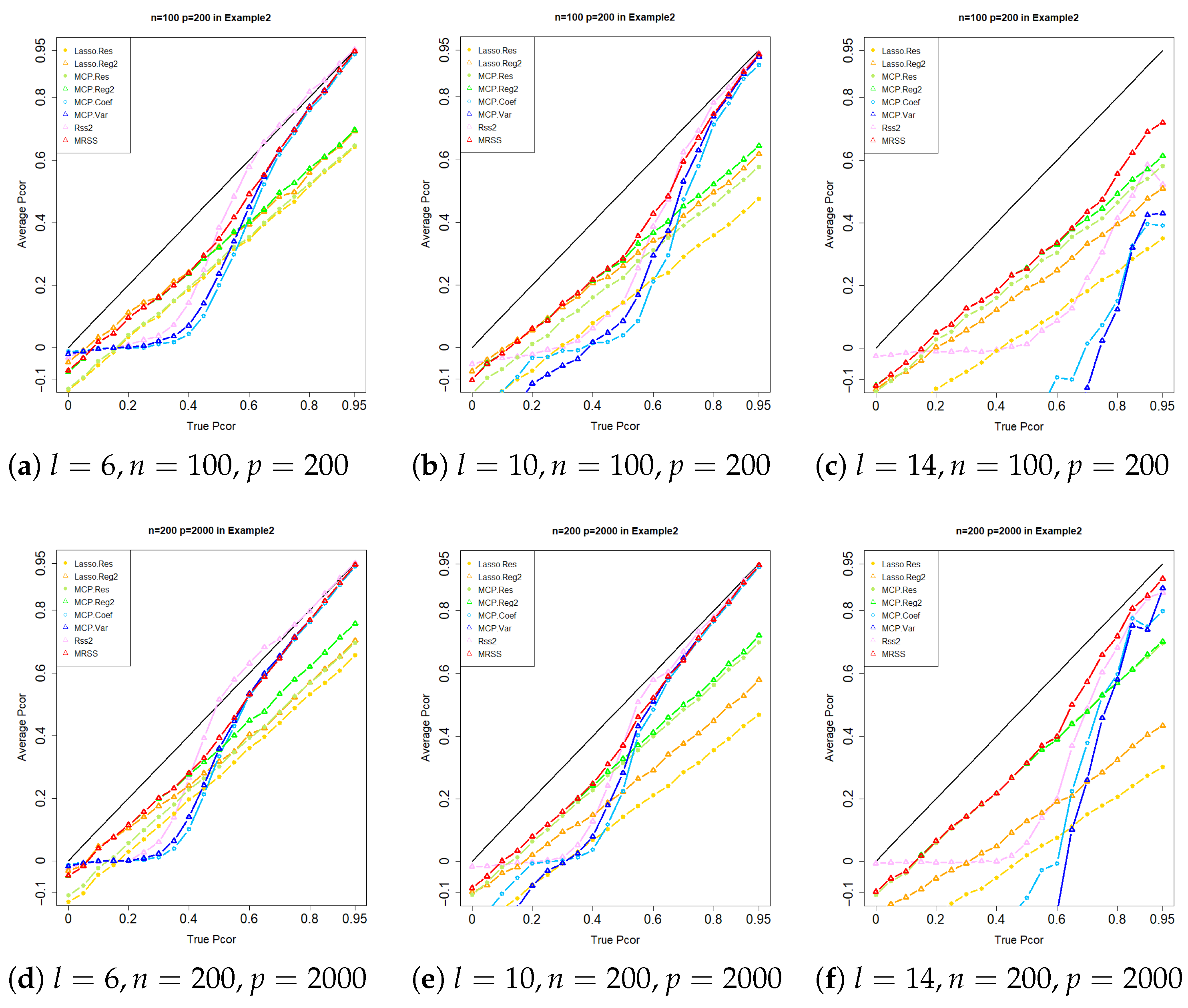
Another indication of the sparsity strength is the number of high correlation controlling variables l. Figure 2 illustrates the performance of the featured algorithms for varying numbers $l=6, 10, 14$. The figure contrasts the average Pcor with the true Pcor for $l=6, 10, 14$ in Example 2 with the first row $n=100, p=200$ and the second $n=200, p=2000$. As l increases, the interference from controlling variables in the estimation process becomes more pronounced, leading to a heightened estimation bias. However, the MRSS algorithm consistently showcases an optimal performance throughout the entire $[0, 1]$ interval. Remarkably, despite encountering a high interference level at $l=14$, MRSS keeps the bias in close alignment with the diagonal, in contrast to its counterparts. Table 4 shows the mean of the MSE and RMSE for $l=6, 10, 14$. As l increases, both the MSE and RMSE of the MRSS algorithm increase, but always remain slightly weaker than optimal in small samples and significantly more optimal than the other algorithms in large samples. These results demonstrate the robustness, stability, and precision advantages of the MRSS algorithm.

Figure 2. Average Pcor against true Pcor for $n=100, p=200$ in the first row and $n=200, p=2000$ in the second row with $l=6, 10, 14$ in Example 2.

Table 4. The mean of MSE ($\times {10}^2$) and RMSE ($\times {10}^2$) for estimated Pcors of real $\mathrm{Pcor}=0, 0.05, \dots , 0.95$ with $l=6, 10, 14$ and ${\sigma }^2=1$ for a large sample size ($n=50, 100$) and small sample size ($n=200, 400$) in Examples 1–4.

Small Sample Size			MSE ($\times {10}^2$)							RMSE ($\times {10}^2$)
		Lasso		MCP						Lasso		MCP
Example	$\mathit{l}$	Res	Reg2	Res	Reg2	Coef	Var	RSS2	MRSS	Res	Reg2	Res	Reg2	Coef	Var	RSS2	MRSS
Example 1	6	9.8	11.2	9.9	9.5	14.4	13.2	11.3	7.4	30.7	31.4	30.8	29.6	32.2	30.9	28.9	25.2
	10	37.1	22.0	33.8	24.1	32.5	31.9	28.9	23.4	59.0	43.8	55.7	46.2	53.8	53.9	50.4	45.4
	14	70.6	37.8	59.6	46.1	91.2	98.5	55.0	47.1	81.2	58.2	72.6	63.6	94.6	98.2	69.6	64.5
Example 2	6	10.2	11.6	10.3	9.9	15.1	13.8	11.6	7.8	31.3	31.9	31.4	30.2	33.1	31.8	29.5	25.9
	10	37.5	22.2	34.4	24.6	32.9	32.3	29.4	24.0	59.4	44.1	56.2	46.8	54.2	54.3	50.8	46.0
	14	71.0	38.2	60.1	46.6	91.5	98.8	55.3	47.5	81.5	58.4	73.0	64.0	94.7	98.4	69.8	64.9
Example 3	6	11.1	12.3	11.3	10.8	16.4	15.1	12.9	9.0	32.6	33.0	32.9	31.6	35.0	33.6	31.4	28.1
	10	39.3	23.4	36.2	26.2	33.8	33.6	30.9	25.7	60.8	45.3	57.9	48.4	55.1	55.5	52.3	47.8
	14	73.0	39.5	62.6	48.8	93.2	100.3	56.7	49.9	82.7	59.6	75.0	65.9	95.6	99.1	70.8	66.9
Example 4	6	15.3	15.6	15.6	14.7	22.1	20.8	18.3	13.8	38.3	37.3	38.6	37.0	41.5	40.4	38.6	35.7
	10	45.4	27.5	43.2	32.0	37.0	37.8	35.4	31.6	65.5	49.5	63.6	54.2	58.2	59.3	56.6	53.8
	14	78.9	43.5	70.9	56.0	98.9	105.3	61.0	57.5	86.3	62.8	80.7	71.5	98.3	101.4	73.9	72.8
Large Sample Size			MSE ($\times {10}^2$)							RMSE ($\times {10}^2$)
		Lasso		MCP						Lasso		MCP
Example	$\mathit{l}$	Res	Reg2	Res	Reg2	Coef	Var	RSS2	MRSS	Res	Reg2	Res	Reg2	Coef	Var	RSS2	MRSS
Example 1	6	2.9	1.9	1.8	1.1	1.6	1.4	1.4	0.5	16.3	12.8	12.4	9.9	9.5	9.0	9.7	6.5
	10	6.8	3.9	1.6	1.5	2.5	2.6	1.7	0.6	24.7	18.4	11.8	11.3	11.8	12.0	10.5	7.0
	14	11.7	6.8	1.6	1.6	12.6	17.9	3.2	0.9	32.2	24.3	11.8	11.9	25.3	29.9	14.1	8.1
Example 2	6	3.1	2.1	2.0	1.3	1.8	1.5	1.5	0.6	17.0	13.5	13.2	10.6	10.2	9.6	9.9	7.1
	10	7.2	4.2	1.8	1.7	2.6	2.8	1.8	0.7	25.4	19.2	12.6	12.2	12.4	12.6	10.8	7.6
	14	12.1	7.2	1.8	1.8	13.1	18.3	3.4	1.0	32.8	25.0	12.7	12.7	26.2	30.7	14.6	8.8
Example 3	6	3.8	2.6	2.6	1.7	2.2	1.9	1.7	0.9	18.8	15.2	15.1	12.4	12.2	11.5	11.0	8.9
	10	8.6	5.3	2.7	2.5	3.6	3.8	2.4	1.3	28.0	21.9	15.7	15.2	16.0	16.2	13.1	10.7
	14	14.4	9.1	3.2	3.1	15.6	21.4	4.5	1.9	36.0	28.5	16.9	16.9	31.0	35.7	17.7	13.0
Example 4	6	8.1	6.1	6.5	5.0	6.0	5.6	4.2	3.9	27.6	23.5	24.7	21.7	22.8	22.2	19.2	19.3
	10	15.7	11.4	8.5	8.1	11.0	11.4	7.3	6.4	38.3	32.3	28.2	27.5	31.6	32.3	25.4	24.9
	14	23.8	17.6	10.7	10.6	29.9	37.4	12.6	9.4	47.0	40.0	31.7	31.5	50.0	55.2	32.6	29.9

4.4. Summaries

Based on numerous simulations, our study examines the practicality and effectiveness of the MRSS algorithm in a variety of scenarios. Through extensive simulations, we provide valuable insights into the accuracy and effectiveness of the MRSS algorithm. We provide empirical evidence that MRSS effectively incorporates the strengths of the MCP.Reg2 and MCP.Var algorithms and reduces the potential weaknesses of Pcor estimation, especially in challenging environments with high-dimensional sparse and non-sparse conditions. For larger sample sizes ($n\ge 100$), the MRSS algorithm reduces the MSE and RMSE by approximately 30–70% compared to other algorithms and effectively controls Pcor estimation errors. For small sample sizes ($n<100$), a reduction of 10–20% is observed in MSE and RMSE for the MRSS algorithm compared to the Res algorithm, an increase of 10–20% compared to Lasso.Reg2, and a slight change compared to other algorithms.

Conducting a sensitivity analysis with various variance and sparsity parameters, the outcomes demonstrate the benefits of the MRSS algorithm in terms of robustness, stability, and accuracy. As the variance increases from 1 to 40, the MSE and RMSE remain consistent for distinct examples and sample sizes. This demonstrates that our MRSS algorithm is remarkably resilient to variability and maintains excellent stability. As the level of sparsity decreases (from Examples 1–4, or from $l=6$ to 14), it is noticeable that the MSE and RMSE of the MRSS algorithm increase, but remain within the same order of magnitude. Even the optimal MRSS algorithms undergo a significant rise in MSE and RMSE for Example 4 and $l=14$, as an escalation of non-sparse and intricate controlling variables brings forth certain systematic errors.

5. Real Data Analysis

A distinguishing feature of financial markets is the observed correlation among the price movements of various financial assets. A prevalent feature entails the existence of a substantial cross-correlation between stock returns’ simultaneous time evolution [29]. In numerous instances, a strong correlation does not necessarily imply a significant direct relationship. For instance, two stocks in the same market may be subject to shared macroeconomic or investor psychology influences. Therefore, to examine the direct correlation between these stocks, it is necessary to eliminate the common drivers represented by the market index. The Pcor meets this requirement by assessing the direct relationship between the two stocks after removing the market impacts of controlling variables. When accurately estimating the Pcor, it is possible to evaluate the impact of diverse factors (e.g., economic sectors, other markets, or macroeconomic factors) on a specific stock. The resulting partial correlation data may be utilised in fields, such as stock market risk management, stock portfolio optimisation, and financial control [7,8]. Moreover, the Pcor can also indicate the interdependence and influence of industries in the context of global integration. These techniques for analysing Pcor can provide valuable information on the correlations between different assets and different sectors of the economy, as they are generalisable and can be applied to other asset types and cross-asset relationships in financial markets. This information is beneficial for practitioners and policymakers.

We chose 100 stocks with substantial market capitalisation and robust liquidity from the Shanghai Stock Exchange (SSE) market. These stocks can comprehensively represent the overall performance of listed stock prices in China’s A-share market. We then downloaded their daily adjusted closing prices from Yahoo Finance from January 2018 to August 2023 and removed the missing data. Here, a sufficient sample size of $n=1075$ was chosen to ensure the effectiveness of algorithms and limit the bias in Pcor estimation. For each pair of the 100 stocks, we estimate their Pcor by setting the remaining stocks as the corresponding controlling variables and construct the estimated Pcor matrix. The Pcor matrix shows the better internal correlation between two stocks after removing the influence of the stock market.

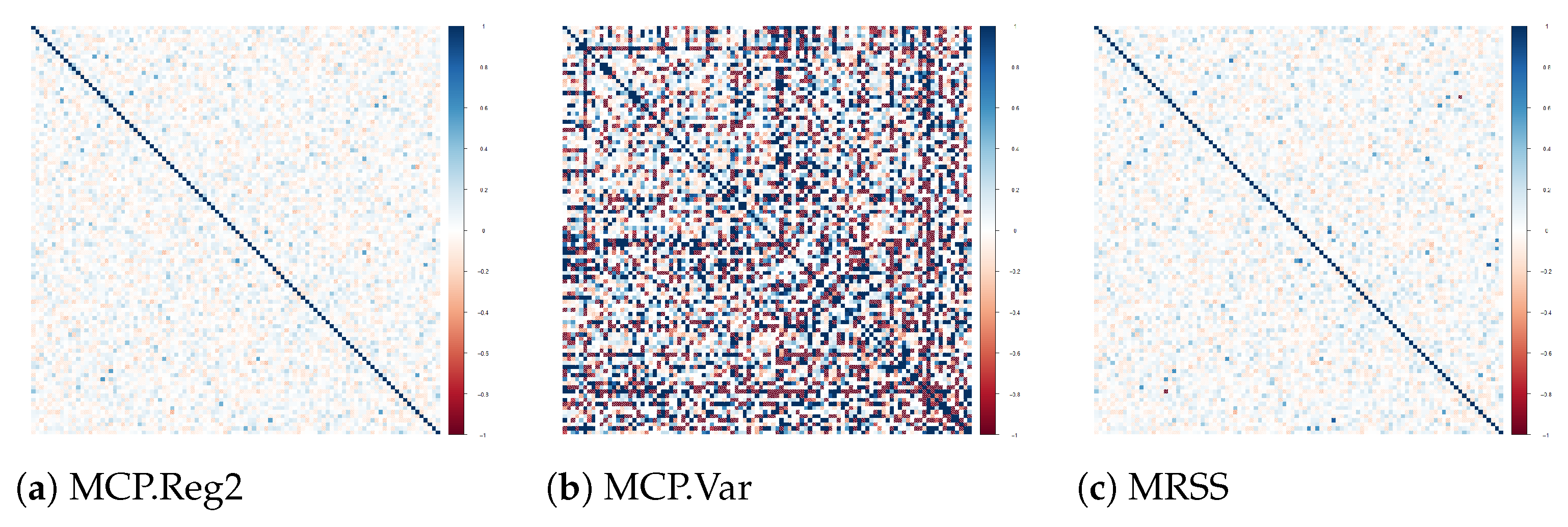
Figure 3 presents the estimated Pcor matrices for 100 stocks from SSE markets using MCP.Reg2, MCP.Var and MRSS algorithms. Blue signifies $\mathrm{Pcor}=1$, while red represents $\mathrm{Pcor}=-1$. Whilst the MCP.Coef, MCP.Var, and RSS2 algorithms all estimate Pcor as 0 when true Pcor approaches 0, our proposed MRSS algorithm resembles the MCP.Reg2, which estimates an accurate Pcor for weak partial correlation. Thus, the MRSS is capable of effectively estimating weak partial correlations. When dealing with high Pcor values and strong partial correlation, we find that the MCP.Var algorithm overestimates Pcor as a result of the divergence in stock prices. For two stocks with a higher stock price, the Pcor estimated by the Var algorithm to be overestimated or even most at 1. MRSS effectively solves this problem. Notably, as a result of incorporating the MCP.Var algorithm, the MRSS algorithm amplifies certain partial correlations that are not significant by MCP.Reg2. These results can also be seen in Table 5. The MRSS estimates these correlations to be stronger partial correlations resulting in improved clarity in the partial correlations.

Figure 3. Estimated Pcor matrix of 100 HKSE stocks, with blue representing $\mathrm{Pcor}=1$ and red representing $\mathrm{Pcor}=-1$.

Table 5. Stock pairs with their sector and Pcor estimates for all the MRSS estimated Pcor $>0.4$ by different algorithms from 100 SSE stocks.

Stock1		Stock2		Lasso		MCP
Symbol	Sector	Symbol	Sector	Res	Reg2	Res	Reg2	Coef	Var	RSS2	MRSS
601398	Financials	601939	Financials	0.526	0.526	0.535	0.535	0.533	0.840	0.527	0.840
600022	Materials	601005	Materials	0.569	0.569	0.581	0.581	0.580	0.769	0.590	0.769
601186	Industrials	601390	Industrials	0.589	0.589	0.566	0.566	0.587	0.748	0.584	0.748
600012	Industrials	601099	Financials	0.405	0.405	0.399	0.399	0.404	0.697	0.414	0.697
601288	Financials	601988	Financials	0.473	0.473	0.476	0.476	0.490	0.646	0.473	0.646
600028	Energy	601857	Energy	0.550	0.550	0.545	0.545	0.569	0.607	0.534	0.607
601098	C.D.	601801	C.D.	0.468	0.468	0.474	0.474	0.475	0.606	0.476	0.606
601328	Financials	601988	Financials	0.357	0.357	0.316	0.316	0.369	0.600	0.322	0.600
600017	Industrials	601880	Industrials	0.372	0.372	0.382	0.382	0.384	0.574	0.394	0.574
600026	Industrials	601872	Industrials	0.590	0.590	0.572	0.573	0.590	1	0.593	0.573
601866	Industrials	601919	Industrials	0.552	0.552	0.545	0.545	0.562	1	0.554	0.545
601179	Industrials	601390	Industrials	0.291	0.291	0.275	0.275	0.285	0.543	0.284	0.543
600011	Utilities	600021	Utilities	0.535	0.535	0.522	0.522	0.535	0.543	0.529	0.543
601333	Industrials	601801	C.D.	0.526	0.526	0.526	0.526	0.525	1	0.528	0.526
600011	Utilities	600027	Utilities	0.514	0.514	0.517	0.517	0.514	1	0.501	0.517
601088	Energy	601666	Energy	0.289	0.289	0.326	0.326	0.359	0.492	0.349	0.492
601288	Financials	601398	Financials	0.353	0.353	0.338	0.338	0.349	0.491	0.339	0.491
601168	Materials	601899	Materials	0.515	0.515	0.490	0.490	0.535	1	0.497	0.490
601186	Industrials	601618	Industrials	0.260	0.260	0.245	0.245	0.250	0.488	0.249	0.488
600018	Industrials	601018	Industrials	0.480	0.480	0.483	0.483	0.486	1	0.485	0.483
600008	Utilities	600012	Industrials	0.319	0.319	0.309	0.309	0.312	0.436	0.304	0.436
601009	Financials	601166	Financials	0.300	0.300	0.298	0.298	0.303	0.427	0.307	0.427
600020	Industrials	601177	Industrials	0.431	0.431	0.430	0.430	0.421	0.422	0.429	0.422
601001	Energy	601137	Materials	0.268	0.268	0.261	0.261	0.283	0.421	0.260	0.421
601519	I.T.	601700	Industrials	0.224	0.224	0.219	0.219	0.217	0.410	0.203	0.410
600017	Industrials	601008	Industrials	0.404	0.404	0.405	0.405	0.403	0.979	0.407	0.405
601318	Financials	601601	Financials	0.414	0.414	0.403	0.403	0.414	1	0.414	0.403

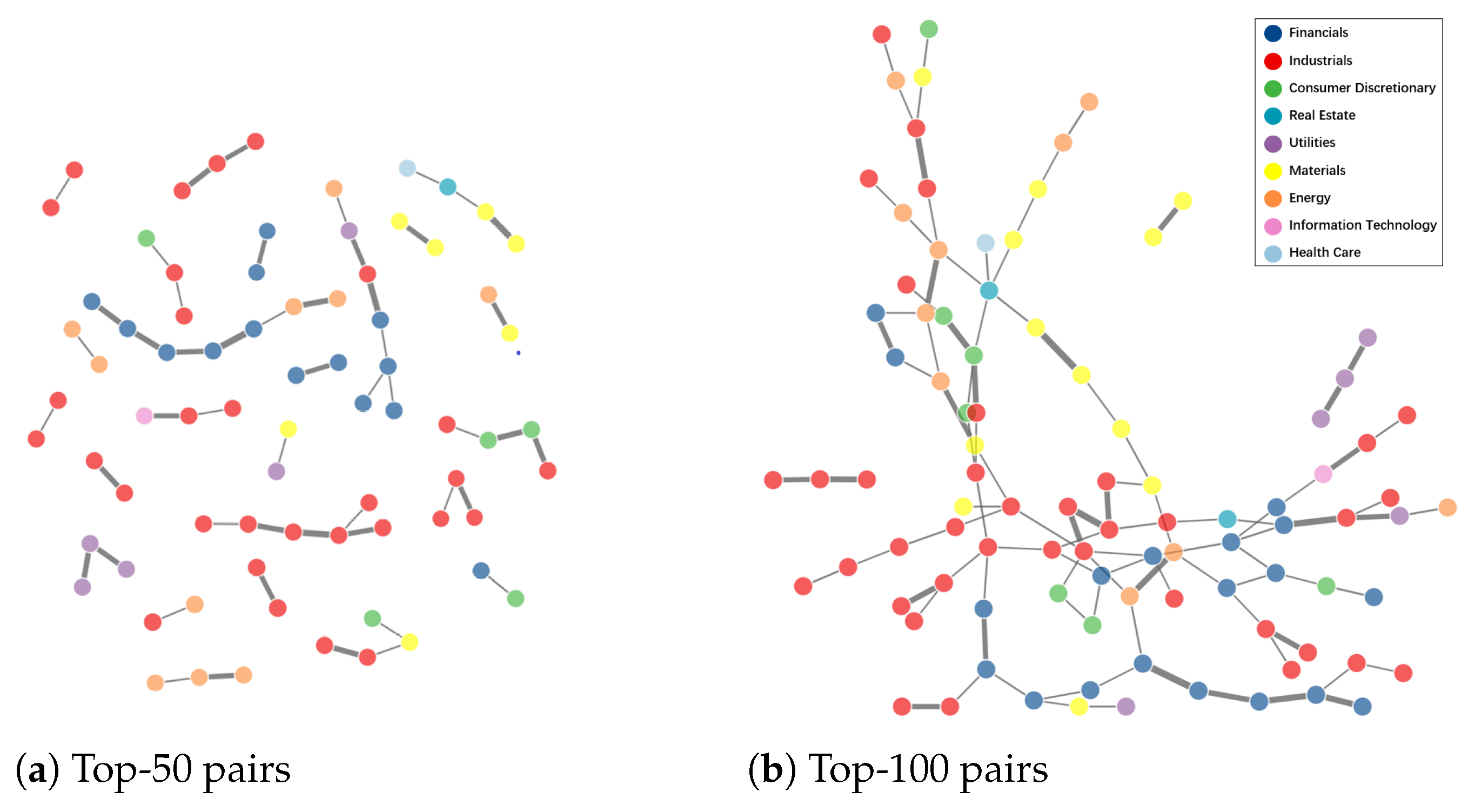
Figure 4 shows the stocks’ Pcor network for the top-100 and top-50 pairs of Pcor estimates by the MRSS algorithm from 100 SSE stocks. The node represents the stock, coloured with its sector. The edge thickness represents the Pcor estimate between two nodes, with the thick-edge Pcor $>0.4$ and the thin-edge Pcor $<0.4$. Table 5 shows the stock pairs with their sector and Pcor estimates for all the MRSS estimated Pcor $>0.4$ from 100 SSE stocks, and Table 6 shows the corresponding stock pairs with their company name, business, and sector. Here, we use industry classifications from the Global Industry Classification Standard (GICS) with Communication Services, Consumer Discretionary (C.D.), Consumer Staples, Energy, Financials, Health Care, Industrials, Information Technology (I.T.), Materials, Real Estate and Utilities. We find that two stocks connected in the partial correlation network with a high Pcor are almost in the same sector and operate in the same business. In addition, high Pcor values may indicate shareholding relationships between companies. For instance, the highly correlated 601398–601939–601288–601988–601328 (financials) are all state-controlled banks that do not have a direct high Pcor link with the city banks 601009–601166 (financials). And, stocks that do not belong to the same industry under a high Pcor may have certain other links behind them, such as 601519 (I.T.)–601700 (industrials) having a common major shareholder. After stripping out the other factors influencing the market, Pcor represents the inherent and intrinsic correlation between two stocks because they are in the same sector.

Figure 4. Stocks’ Pcor network for the top-100 and top-50 pairs of Pcor estimates by MRSS algorithm from 100 SSE stocks. The node represents the stock, coloured with its sector. The edge thickness represents the Pcor estimate between two nodes, with the thick edge Pcor $>0.4$ and the thin edge Pcor $<0.4$.

Table 6. Stock pairs with their company name, business, and sector for all the MRSS estimated Pcor $>0.4$ from 100 SSE stocks.

Symbol	Company	Business	Sector	Symbol	Company	Business	Sector
601098	South central Media	Media	C.D.	601801	Anhui Xinhua Media	publishing	C.D.
600028	Sinopec	Refining and Trading	Energy	601857	PetroChina	Refining and Trading	Energy
601088	China Shenhua Energy	Coal Mining	Energy	601666	Pingdingshan Tianan Coal Mining	Coal Mining	Energy
601001	Datong Coal Industry	Coal Mining	Energy	601137	Ningbo Boway Alloy Material	Industrial Metals	Materials
601398	Industrial and Commercial Bank of China	Banks	Financials	601939	China Construction Bank	Banks	Financials
601288	Agricultural Bank of China	Banks	Financials	601988	Bank of China	Banks	Financials
601328	Bank of Communications	Banks	Financials	601988	Bank of China	Banks	Financials
601288	Agricultural Bank of China	Banks	Financials	601398	Industrial and Commercial Bank of China	Banks	Financials
601009	Bank of Nanjing	Banks	Financials	601166	Industrial Bank of China	Banks	Financials
601318	Ping An Insurance of China	Insurance	Financials	601601	China Pacific Insurance	Insurance	Financials
601186	China Railway Construction	Infrastructure	Industrials	601390	China Railway Engineering Group	Infrastructure	Industrials
600012	Anhui Expressway	Railway and Highway	Industrials	601099	China Pacific Insurance	certificate	Financials
600017	Rizhao Port	Shipping Ports	Industrials	601880	Dalian Port	Shipping Ports	Industrials
600026	China Shipping Development	Shipping Ports	Industrials	601872	China Merchants Energy Shipping	Shipping Ports	Industrials
601866	China Shipping Container Lines	Shipping Ports	Industrials	601919	China Ocean Shipping	Shipping Ports	Industrials
601179	China Xidian Electric	Grid Equipment	Industrials	601390	China Railway Engineering	Infrastructure	Industrials
601333	Guangshen Railway	Railway and Highway	Industrials	601801	Anhui Xinhua Media	publishing	C.D.
601186	China Railway Construction	Infrastructure	Industrials	601618	Metallurgical Corporation of China	Professional Engineering	Industrials
600018	Shanghai International Port Group	Shipping Ports	Industrials	601018	Ningbo Port	Shipping Ports	Industrials
600020	Zhongyuan Expressway	Railway and Highway	Industrials	601177	Hangzhou Advance Gearbox	machine	Industrials
600017	Rizhao Port	Shipping Ports	Industrials	601008	Lianyungang Port	Shipping Ports	Industrials
601519	Shanghai DZH	Software Development	I.T.	601700	Changshu Fengfan Power Equipment	Grid Equipment	Industrials
600022	Jinan Iron and Steel	Plain Steel	Materials	601005	Chongqing Iron and Steel	Plain Steel	Materials
601168	Western Mining	Industrial Metals	Materials	601899	Zijin Mining	Industrial Metals	Materials
600011	Huaneng Power International	Electricity	Utilities	600021	Shanghai Electric Power	Electricity	Utilities
600011	Huaneng Power International	Electricity	Utilities	600027	Huadian Power International	Electricity	Utilities
600008	Beijing Capital	Water	Utilities	600012	Anhui Expressway	Railway and Highway	Industrials

As societies become increasingly integrated, the productive activities of different industries become interdependent and interact with each other. Categorising a company into only one industry does not reflect its overall performance and associated risks. Many listed companies in the stock market belong to conglomerates and operate in different industry sectors, so it is natural for the performance of these companies to be affected by multiple industries. Therefore, we will also find that Pcor, apart from showing the correlation between industries, will also reveal the correlation between two industries that are linked together by two stocks in different industries. For example, the partial correlation between the Bank of Communications (601328) and PetroChina (601857) with Pcor $=0.258$ links the Energy (600028–601857 in orange) and Financial (601398–601939–601288–601988–601328 in dark blue) sectors of state-owned assets.

Overall, the MRSS algorithm amalgamates the characteristics of MCP.Reg2 and MCP.Var, enhancing the estimation of strong partial correlations, while effectively estimating those weak partial correlations, ultimately revealing the stock correlations.

6. Conclusions

This paper presents a novel minimum residual sum of squares (MRSS) algorithm for estimating partial correlation coefficients. Its purpose is to reduce the estimation bias of positive partial correlation coefficients in high-dimensional settings under both sparse and non-sparse conditions. The MRSS algorithm is effective in mitigating a Pcor estimation bias by synergistically harnessing the strengths of the Coef, Reg2, and Var algorithms. We also discuss the MRSS algorithm mathematical foundation and its performance in various scenarios compared to some existing algorithms. Through rigorous simulations and real data analysis, it becomes evident that the MRSS algorithm consistently outperforms its constituent and listed algorithms, particularly in challenging environments characterised by non-sparse conditions and high dimensionality. The sensitivity analysis with variance and sparsity parameters demonstrate the robustness, stability, and precision advantages of the MRSS algorithm. Further evidence of the effectiveness of the MRSS algorithm in the correlation analysis of stock data is provided by real data analyses.

7. Future Work

Our proposed MRSS algorithm combines the benefits of two existing algorithms by reducing the total squared residuals and enhancing the accuracy of Pcor estimation. In upcoming studies, we may explore the integration of additional algorithms by minimising the RSS to achieve a greater amalgamation of benefits from various algorithms and improve the estimation accuracy of the integrated algorithm. Reducing the computational complexity of our minimised RSS integration algorithm to decrease computing time represents a core issue in future research. Additionally, conducting in-depth theoretical research on MRSS algorithms, including a proof analysis of consistency and convergence, will be an essential direction for our next steps. Further refinement of theoretical proofs and an in-depth investigation of error convergence speed may uncover reasons for the systematic estimation bias that cannot be ignored when Pcor is positive in all current algorithms. Meanwhile, expanding the use of the MRSS algorithm to a wider range of fields is a focal point of our future research. Concerning financial data, we intend to thoroughly examine the biased correlations between financial data besides stocks and advise on relevant policies.

References

- Tabachnick; Barbara, G.; Linda, S.F.; Jodie, B.U. Using Multivariate Statistics, 6th ed.; Pearson: Boston, MA, USA, 2013. [Google Scholar]
- Huang, Y.; Chang, X.; Zhang, Y.; Chen, L.; Liu, X. Disease characterization using a partial correlation-based sample-specific network. Brief. Bioinform. 2021, 22, bbaa062. [Google Scholar] [CrossRef]
- Peng, J.; Wang, P.; Zhou, N.; Zhu, J. Partial correlation estimation by joint sparse regression models. J. Am. Stat. Assoc. 2009, 104, 735–746. [Google Scholar] [CrossRef] [PubMed]
- De La Fuente, A.; Bing, N.; Hoeschele, I.; Mendes, P. Discovery of meaningful associations in genomic data using partial correlation coefficients. Bioinformatics 2004, 20, 3565–3574. [Google Scholar] [CrossRef] [PubMed]
- Marrelec, G.; Kim, J.; Doyon, J.; Horwitz, B. Large-scale neural model validation of partial correlation analysis for effective connectivity investigation in functional MRI. Hum. Brain Mapp. 2009, 30, 941–950. [Google Scholar] [CrossRef] [PubMed]
- Wang, G.J.; Xie, C.; Stanley, H.E. Correlation structure and evolution of world stock markets: Evidence from Pearson and partial correlation-based networks. Comput. Econ. 2018, 51, 607–635. [Google Scholar] [CrossRef]
- Kenett, D.Y.; Tumminello, M.; Madi, A.; Gur-Gershgoren, G.; Mantegna, R.N.; Ben-Jacob, E. Dominating clasp of the financial sector revealed by partial correlation analysis of the stock market. PLoS ONE 2010, 5, e15032. [Google Scholar] [CrossRef]
- Kenett, D.Y.; Huang, X.; Vodenska, I.; Havlin, S.; Stanley, H.E. Partial correlation analysis: Applications for financial markets. Quant. Finance 2015, 15, 569–578. [Google Scholar] [CrossRef]
- Michis, A.A. Multiscale partial correlation clustering of stock market returns. J. Risk Financ. Manag. 2022, 15, 24. [Google Scholar] [CrossRef]
- Singh, V.; Li, B.; Roca, E. Global and regional linkages across market cycles: Evidence from partial correlations in a network framework. Appl. Econ. 2019, 51, 3551–3582. [Google Scholar] [CrossRef]
- Epskamp, S.; Fried, E.I. A tutorial on regularized partial correlation networks. Psychol. Methods 2018, 23, 617–634. [Google Scholar] [CrossRef]
- Williams, D.R.; Rast, P. Back to the basics: Rethinking partial correlation network methodology. Brit. J. Math. Stat. Psy. 2020, 73, 187–212. [Google Scholar] [CrossRef] [PubMed]
- Waldorp, L.; Marsman, M. Relations between networks, regression, partial correlation, and the latent variable model. Multivariate Behav. Res. 2022, 57, 994–1006. [Google Scholar] [CrossRef]
- Gvozdarev, A.; Parovik, R. On the relationship between the fractal dimension of geomagnetic variations at Altay and the space weather characteristics. Mathematics 2023, 11, 3449. [Google Scholar] [CrossRef]
- Khare, K.; Oh, S.Y.; Rajaratnam, B. A convex pseudolikelihood framework for high dimensional partial correlation estimation with convergence guarantees. J. R. Stat. Soc. B 2015, 77, 803–825. [Google Scholar] [CrossRef]
- Kim, S. ppcor: An R package for a fast calculation to semi-partial correlation coefficients. Commun. Stat. Appl. Methods 2015, 22, 665. [Google Scholar] [CrossRef] [PubMed]
- Huang, Z.; Deb, N.; Sen, B. Kernel partial correlation coefficient—A measure of conditional dependence. J. Mach. Learn. Res. 2022, 23, 9699–9756. [Google Scholar]
- Van Aert, R.C.; Goos, C. A critical reflection on computing the sampling variance of the partial correlation coefficient. Res. Synth. Methods 2023, 14, 520–525. [Google Scholar] [CrossRef]
- Hu, H.; Qiu, Y. Inference for nonparanormal partial correlation via regularized rank based nodewise regression. Biometrics 2023, 79, 1173–1186. [Google Scholar] [CrossRef]
- Cox, D.R.; Wermuth, N. Multivariate Dependencies–Models, Analysis and Interpretation; Chapman and Hall: London, UK, 1996. [Google Scholar]
- Tibshirani, R. Regression shrinkage and selection via the lasso. J. R. Stat. Soc. B 1996, 58, 267–288. [Google Scholar] [CrossRef]
- Owen, A.B. A robust hybrid of lasso and ridge regression. Contemp. Math. 2007, 443, 59–72. [Google Scholar]
- Fan, J.; Li, R. Variable selection via nonconcave penalized likelihood and its oracle properties. J. Am. Stat. Assoc. 2001, 96, 1348–1360. [Google Scholar] [CrossRef]
- Zou, H.; Hastie, T. Regularization and variable selection via the elastic net. J. R. Stat. Soc. B. 2005, 67, 301–320. [Google Scholar] [CrossRef]
- Tibshirani, R.; Saunders, M.; Rosset, S.; Zhu, J.; Knight, K. Sparsity and smoothness via the fused lasso. J. R. Stat. Soc. B. 2005, 67, 91–108. [Google Scholar] [CrossRef]
- Zhang, C.H. Nearly unbiased variable selection under minimax concave penalty. Ann. Stat. 2010, 38, 894–942. [Google Scholar] [CrossRef] [PubMed]
- Wang, H. Coordinate descent algorithm for covariance graphical lasso. Stat. Comput. 2014, 24, 521–529. [Google Scholar] [CrossRef]
- Fan, J.; Fan, Y.; Lv, J. High dimensional covariance matrix estimation using a factor model. JoE. 2008, 147, 186–197. [Google Scholar] [CrossRef]
- Elton, E.J.; Gruber, M.J.; Brown, S.J.; Goetzmann, W.N. Modern Portfolio Theory and Investment Analysis; John Wiley and Sons: Hoboken, NJ, USA, 2009. [Google Scholar]
Disclaimer/Publisher’s Note: The statements, opinions and data contained in all publications are solely those of the individual author(s) and contributor(s) and not of MDPI and/or the editor(s). MDPI and/or the editor(s) disclaim responsibility for any injury to people or property resulting from any ideas, methods, instructions or products referred to in the content. |
© 2023 by the authors. Licensee MDPI, Basel, Switzerland. This article is an open access article distributed under the terms and conditions of the Creative Commons Attribution (CC BY) license (https://creativecommons.org/licenses/by/4.0/).