Generalized de Boor–Cox Formulas and Pyramids for Multi-Degree Spline Basis Functions

Abstract

The conventional B-splines possess the de Boor–Cox formula, which relates to a pyramid algorithm. However, for multi-degree splines, a de Boor–Cox-type evaluation algorithm only exists in some special cases. This paper considers any multi-degree spline with arbitrary degree and continuity, and provides two generalized de Boor–Cox-type relations. One uses several lower degree polynomials to build a combination to evaluate basis functions, whose form is similar to using the de Boor–Cox formula several times. The other is a linear combination of two functions out of the recursive definition, which keeps the combination coefficient polynomials of degree 1, so it is more similar to the de Boor–Cox formula and can be illustrated by several pyramids with different heights. In the process of calculating the recursions, a recursive representation using the Bernstein basis is used and numerically analyzed.

1. Introduction

B-splines are well-established tools in computer-aided geometric design. Their basic functions build the unique normalized B-basis in their spanned space of piecewise polynomials, which has optimal shape-preserving properties [1]. Multi-degree splines (MD-splines for short), also called changeable-degree splines, allow different degrees for different segments. In their spanned space of piecewise polynomials with varying degrees, their basic functions also construct the unique normalized B-basis [2]. Therefore, they can be viewed as a direct extension of B-splines.

For MD-splines, the use of splines with varying degrees were investigated by [3] as a tool for approximation. Some variable-degree polynomial functions in [4,5] were constructed for shape-preserving interpolation and more theories were proposed in [6,7,8], in [9] the concept of multi-degree splines was proposed and some MD-spline curves of degree 1, 2 and 3 were built. In [10], a two-degree-spline basis is provided for dividing the process of degree elevation of B-spline into corner-cutting form. In [2,11], two types of MD-splines with different continuities were defined, and [12] deals with an explicit expression for MD-splines. The MD-spline degree-elevation property is provided in [13]. The definition of MD-splines is improved in [14]; two extended partitions are made ingeniously to unify the two types of MD-splines. Such extended partitions for B-splines were proposed in [15]. The support of each basis function is easily determined by the indexes of two extended partitions, and, using this configuration, arbitrary continuity MD-splines can be created. Recent references offer several numerical algorithms due to the inefficiency of the integral definition for MD-splines in numerical calculation. They employ simpler bases to express MD-splines and to compute the representation matrix. In [16], the continuity constraints between spline pieces were collected in a matrix and then its null space was computed by recurrence. In [17], it was proven that the output of this algorithm is exactly the basis of MDB-splines and a Chebyshevian extension of the construction was presented in [18]. The algorithm in [19] repeats the reverse knot insertion (RKI) process to evaluate the transition matrix. An improved version of the algorithm in [19] is outlined in [20]. it is a numerically stable method, because it avoids the derivative operations and minimizes the number of floating-point operations.

B-splines $F_{i,n}$ are recursively computed by applying the de Boor–Cox formula in [21,22], which is related to a pyramid algorithm in [23], namely,

$$F_{i,n}\left(t\right)=\frac{t-t_i}{t_{i+n}-t_i}{F}_{i,n-1}\left(t\right)+\frac{t_{i+n+1}-t}{t_{i+n+1}-t_{i+1}}{F}_{i+1,n-1}\left(t\right)$$

(1)

In the formula, a B-spline of degree n is represented by two B-splines of degree $n-1$, where the combination coefficients are both polynomials of degree 1. According to [24,25], the MD-splines build a de Boor–Cox-type formula if the continuity orders between neighboring pieces of different degrees are no more than 1. For general cases, the de Boor–Cox-type formula does not exist [14].

Our work is focused on more generalized de Boor–Cox-type relations for arbitrary-degree MD-splines with any continuity orders and provides two generalized forms. The first form uses the de Boor–Cox formula several times. A B-spline basis function of degree n is represented as a combination of $s+1$ B-splines of degree $n-s$ with polynomial coefficients ${\sigma }_{i,n-s}\left(t\right),{\sigma }_{i+1,n-s}\left(t\right),\dots ,{\sigma }_{i+s,n-s}\left(t\right)$ of degree s, i.e.

$$F_{i,n}\left(t\right)={\sigma }_{i,n-s}\left(t\right)F_{i,n-s}\left(t\right)+{\sigma }_{i+1,n-s}\left(t\right)F_{i+1,n-s}\left(t\right)+\dots +{\sigma }_{i+s,n-s}\left(t\right)F_{i+s,n-s}\left(t\right)$$

(2)

For MD-splines, each function $N_{i,n},i=D-n+1,\dots ,\mathcal{K}$ at level n can be represented by functions at recursive level $n-s$, where these functions should be $C^0$ continuous or discontinuous at knots in their support intervals. On each interval, the sum of the degree of a function involved in the recurrence is similar to (2) and that of its coefficient polynomial is equal to the degree of $N_{i,n}$. We provide an algorithm to calculate these coefficient polynomials. In the meantime, functions at recursive level $n-1$ can also be represented by these functions at recursive level $n-s$, allowing the first form to be translated into a new form. In this new form, a function $N_{i,n}$ at recursive level n is represented by a combination of $N_{i,n-1}$, $N_{i+1,n-1}$ and functions at recursive level $n-s$, where the coefficient polynomials of $N_{i,n-1}$, and $N_{i+1,n-1}$ are bothpolynomials of degree 1. In the second form, a function $N_{i,n}$ at recursive level n is represented by two functions with combination coefficient polynomials of degree 1. The left coefficient polynomial is the result of subtracting the left endpoint of $N_{i,n}$ from t, and the right coefficient polynomial is the result of subtracting t from the right endpoint of $N_{i,n}$. Two representation functions are not in the integral recursion, but they can be constructed using knots derivative information of functions at recursive level $n-1,n-2,...,1$. We present a building method based on the Taylor expansion of polynomials which demonstrates the theoretical viability of this form. If we replace functions that are not applicable to de Boor–Cox-type formulas with their construction polynomials in the recursion of MD-spline basis, then any function can be evaluated using this form formula. Multiple pyramids of varying heights can be used to depict this recurrence. To obtain the two forms for MD-splines, we offer a recursive method to evaluate the representation matrix between the MD-spline basis and Bernstein basis, and design some numerical experiments for it. This method utilizes the integral property of Bernstein polynomials and possesses sufficient numerical accuracy and efficiency.

The remainder of this paper is organized as follows: Section 2 reviews the necessary definitions of MD-splines. Section 3 provides a recursive method by Bernstein representation and contains some numerical experiments. Section 4 reveals general recursive relations of the MD-spline basis and constructs de Boor–Cox-type formula. Finally, this paper is concluded with some conclusion.

2. MD-Spline Basis Review

In the following, we will recall some concepts of MD-splines given in [9,14]. MD-spline basis functions are piecewise polynomials defined on a partition of an interval, which is determined by a breakpoint sequence $\mathit{T}$, a degree sequence $\mathit{G}$, and a sequence $\mathit{K}$ containing the orders of regularity.

Let $\mathit{T}:={\left\{t_i\right\}}_{i=0}^{q+1}$, $a=t_0<t_1<\dots <t_q<t_{q+1}=b$ be a strictly increasing partition of a given interval $\mathit{I}:=[a,b]$. If $d_i>0,i=0,\dots ,q$ is the degree of the MD-spline on $[t_i,t_{i+1})$, then let $\mathit{G}:={\left\{d_i\right\}}_{i=0}^q$ be the degree sequence and $D=\max \left\{d_i\right\},0⩽i⩽q$. Finally, the entries of the order sequence $\mathit{K}:={\left\{k_i\right\}}_{i=1}^q$, which describe the required continuity at breakpoints $t_i,i=1,2,\dots ,q$, are defined as follows:

$$k_i⩽\left\{\begin{array}{cc}{d}_{i-1},\hfill & \hfill if{d}_{i-1}=d_i,\\ \min \left\{d_i,d_{i-1}\right\},\hfill & \hfill if{d}_{i-1}\ne d_i.\end{array}\right.$$

(3)

There are two extended partitions of $\mathit{T}$ to determine the support intervals. The left extended partition is

$$\mathit{S}:=\left\{s_1,s_2,\dots ,s_{\mathcal{K}}\right\}:=\{\underset{d_0+1times}{\underbrace{t_0,\dots ,t_0}},\underset{d_1-k_{1}times}{\underbrace{t_1,\dots ,t_1}},\dots ,\underset{d_q-k_{q}times}{\underbrace{t_q,...,t_q}}\},$$

(4)

and the right one is

$$\mathit{X}:=\left\{x_1,x_2,\dots ,x_{\mathcal{K}}\right\}:=\{\underset{d_0-k_{1}times}{\underbrace{t_1,\dots ,t_1}},\dots ,\underset{d_{q-1}-k_{q}times}{\underbrace{t_q,\dots ,t_q}},\underset{d_q+1times}{\underbrace{t_{q+1},\dots ,t_{q+1}}}\},$$

(5)

where $\mathcal{K}:=d_0+{\sum }_{i=1}^q(d_i-k_i)+1=d_q+{\sum }_{i=1}^q(d_{i-1}-k_i)+1$.

Figure 1 shows an example for illustrating the left and right extended partitions. Here, $\mathit{T}:={\left\{t_i\right\}}_{i=0}^5$, $\mathit{G}:=\left\{3,3,4,5,5\right\}$, $\mathit{K}:=\left\{2,2,3,4\right\}$, and $\mathcal{K}=10$.

Figure 1. Original partition $\mathit{T}$, left and right extended partitions $\mathit{S}$ and $\mathit{X}$, respectively.

The relation of indexes is noted by function p. In detail, $p\left(s_i\right)$ is the index of the corresponding breakpoint of $s_i$ in $\mathit{T}$ and $p\left(x_i\right)$ is the index of the corresponding breakpoint $x_i$ in $\mathit{T}$. That is, $t_{p\left(s_i\right)}=s_i$, and $t_{p\left(x_i\right)}=x_i$. For example, in Figure 1, since $s_6=s_7=t_2$, $p\left(s_6\right)=p\left(s_7\right)=2$. Since $x_3=t_3$, $p\left(x_3\right)=3$.

Definition 1

(Multi-degree spline basis). For $n=0,1,...,D$, functions in ${\left\{N_{i,n}\left(t\right)\right\}}_{i=D-n+1}^{\mathcal{K}}$ are generated recursively over $\mathit{T}$, $\mathit{G}$ and $\mathit{K}$. The final sequence ${\left\{N_{i,D}\left(t\right)\right\}}_{i=1}^{\mathcal{K}}$ is a MD-spline basis, given by

$$N_{i,n}\left(t\right)=\left\{\begin{array}{cc}0,\hfill & d_j<D-n,\hfill \\ \left\{\begin{array}{cc}1\hfill & t\in [t_j,t_{j+1})\hfill \\ 0\hfill & otherwise\hfill \end{array}\right.,\hfill & d_j=D-n,\hfill \\ {\int }_{-\infty }^t({\delta }_{i,n-1}{N}_{i,n-1}\left(y\right)-{\delta }_{i+1,n-1}{N}_{i+1,n-1}\left(y\right))dy,\hfill & d_j>D-n.\hfill \end{array}\right.$$

(6)

for each nontrivial interval $[t_j,t_{j+1})\subseteq [s_i,x_{i-D+n})=[t_{p\left(s_i\right)},t_{p\left(x_{i-D+n}\right)})$, where

$${\delta }_{i,n}:={\left({\int }_{-\infty }^{+\infty }{N}_{i,n}\left(y\right)dy\right)}^{-1}$$

In addition, when $N_{i,n}=0$, we set

$${\int }_{-\infty }^t{\delta }_{i,n}{N}_{i,n}\left(y\right)dy=\left\{\begin{array}{cc}0\hfill & t<s_i,\hfill \\ 1\hfill & t\ge s_i.\hfill \end{array}\right.$$

MD-spline basis ${\left\{N_{i,D}\left(t\right)\right\}}_{i=1}^{\mathcal{K}}$ possesses some properties such as a B-spline basis:

• Local support: $N_{i,D}\left(t\right)=0$ for $t\notin [s_i,x_i]$.
• Positivity: $N_{i,D}\left(t\right)>0$ for $t\in (s_i,x_i)$.
• End point: $N_{i,D}\left(t\right)$ vanishes exactly $d_{p\left(s_i\right)}-max\left\{j\ge 0|s_i=s_{i+j}\right\}$ times at $s_i$, and $d_{p\left(x_i\right)-1}-max\left\{j\ge 0|x_{i-j}=x_i\right\}$ at $x_i$.
• Partition of unity: ${\sum }_i^{\mathcal{K}}{N}_{i,D}\left(t\right)\equiv 1$ for all $t\in [a,b].$

Some properties of functions $N_{i,n}$, $i=D-n+1,D-n+2,\dots ,\mathcal{K}$ for any $0⩽n⩽D$ are as follows:

• Support interval: the support interval of $N_{i,n}\left(t\right)$ is $[s_i,x_{i-D+n}).$
• Degree: on interval $[t_j,t_{j+1})\subseteq [s_i,x_{i-D+n})$ with $s_i<x_{i-D+n}$, the degree of $N_{i,n}\left(t\right)$ equals to $d_j+n-D$ when $n\ge D-d_j$.
• Continuity: at knot $t_j$, $t_j\in (s_i,x_{i-D+n})$ with $s_i<x_{i-D+n}$, $N_{i,n}\left(t\right)$ is $C^{k_j+n-D}$-continuous when $n\ge D-k_j$.

In [24], $C^k$ MD-splines are defined to describe some particular MD-spline bases, such as $C^0$, $C^1$ MD-splines.

Definition 2

($C^k$ multi-degree spline basis). An MD-spline basis is said to be a $C^k$ MD-spline basis if its functions are, at most, $C^k$ continuous at the joins between pieces of different degrees.

In the example of Figure 1, as $d_0=d_1$, $d_3=d_4$, we do not need to consider the continuity at $t_1$ and $t_4$. Therefore, functions in this basis will be $C^2$-continuous at the join between $[t_0,t_2)$ and $[t_2,t_3)$, and be $C^3$-continuous at the join between $[t_2,t_3)$ and $[t_3,t_5)$. Therefore, the corresponding MD-spline basis will be a $C^3$ MD-spline basis.

3. Recursive Method

As Bernstein polynomials of degree n form a basis of the space ${\mathcal{P}}_n$ of polynomials of degree at most n, functions in ${\left\{N_{i,n}\left(t\right)\right\}}_{i=D-n+1}^{\mathcal{K}}$ can be represented by Bernstein polynomials with different degrees. Thus, the recursive process for defining an MD-spline basis can be performed from these Bernstein polynomials.

3.1. Bernstein Representation

Bernstein polynomials [26] of degree n on interval $[t_j,t_{j+1}]$ are defined as

$$b_{i,n}^j\left(t\right):=\frac{\left(\begin{array}{c}n\\ i\end{array}\right){\left(t-t_j\right)}^i{\left(t_{j+1}-t\right)}^{n-i}}{{\left(t_{j+1}-t_j\right)}^n},i=0,1,\dots ,n.$$

(7)

Let

$${\mathit{B}}_n^j\left(t\right):={\left(b_{0,n}^j\left(t\right),b_{1.n}^j\left(t\right),\dots ,b_{n,n}^j\left(t\right)\right)}^T.$$

(8)

Then, each function $N_{i,n}$, $i=D-n+1,D-n+2,\dots ,\mathcal{K}$ and $n=0,1,\dots ,D$ can be linearly represented as

$$N_{i,n}\left(t\right)=a_{i,n}^{0,j}{b}_{0,n}^j\left(t\right)+a_{i,n}^{1,j}{b}_{1,n}^j\left(t\right)+\dots +a_{i,n}^{n,j}{b}_{n,n}^j\left(t\right),$$

(9)

where $a_{i,n}^{0,j},a_{i,n}^{1,j},\dots ,a_{i,n}^{n,j}$ are some constants that are not all zero, and this equation can also be written as

$$N_{i,n}\left(t\right)={\mathit{A}}_{i,n}^j{\mathit{B}}_{d_j+n-D}^j\left(t\right),t\in [t_j,t_{j+1}),j=p\left(s_i\right),p\left(s_i\right)+1,\dots ,p\left(x_{i+D-n}\right)-1,$$

(10)

where ${\mathit{A}}_{i,n}^j=\left(a_{i,n}^{0,j},a_{i,n}^{1,j},\dots ,a_{i,n}^{n,j}\right)$ is called the Bernstein representation vector of function $N_{i,n}$ on $[t_j,t_{j+1})$.

On the support interval of $N_{i,n}$, consistent with the previous settings, the number of elements in $\mathit{T}$ is $q+2$. For each n, ${\mathbb{B}}_n$ stands for the whole set of Bernstein polynomials:

$${\mathbb{B}}_n:=\left(\begin{array}{c}{\mathit{B}}_{d_1+n-D}^1\left(t\right)\\ {\mathit{B}}_{d_2+n-D}^2\left(t\right)\\ ⋮\\ {\mathit{B}}_{d_{l-1}+n-D}^{q+1}\left(t\right)\end{array}\right).$$

(11)

Let

$${\overrightarrow{\mathcal{A}}}_{i,n}:=\left(\mathbf{0},\dots ,\mathbf{0},{\mathit{A}}_{i,n}^{p\left(s_i\right)},{\mathit{A}}_{i,n}^{p\left(s_i\right)+1},\dots ,{\mathit{A}}_{i,n}^{p\left(x_{i-D+n}\right)-1},\mathbf{0},\dots ,\mathbf{0}\right).$$

(12)

Then

$$N_{i,n}\left(t\right)={\overrightarrow{\mathcal{A}}}_{i,n}{\mathbb{B}}_n,$$

(13)

and the corresponding representation matrix is

$$\mathit{N}=\mathit{M}{\mathbb{B}}_n,$$

(14)

where

$$\begin{array}{cc}\hfill & \mathit{N}:={\left(N_{D-n+1,n}\left(t\right),N_{D-n+2,n}\left(t\right),\dots ,N_{\mathcal{K},n}\left(t\right)\right)}^T,\hfill \\ \hfill & \mathit{M}:={\left(\begin{array}{c}{\overrightarrow{\mathcal{A}}}_{D-n+1,n}\\ ⋮\\ {\overrightarrow{\mathcal{A}}}_{\mathcal{K},n}\end{array}\right)}_{(\mathcal{K}-D+n)\times {\sum }_{j=1}^{q+1}(d_j+n-D+1)}\hfill \end{array}$$

(15)

Compared with the representation matrix in [19], matrix $\mathit{M}$ represents functions in ${\left\{N_{i,n}\right\}}_{i=D-n+1}^{\mathcal{K}}$ at each recursive level n.

Definition 3

($C^k$ function). A function defined over $\mathit{T}$, $\mathit{G}$ and $\mathit{K}$ is called a $C^k$ function if it is at most $C^k$ continuous at breakpoints within its support interval.

$C^k$ functions are not equivalent to functions in a $C^k$ MD-spline basis, a $C^k$ MD-spline basis only requires continuity at the join of different degrees. For example, a $C^0$ MD-spline basis may contain B-splines; however, B-splines are not $C^0$ continuous at their internal breakpoints. A $C^0$ MD-spline basis has some particular properties, such as the integrals of functions in it can be computed easily, which is used in [20]. $C^0$ functions are also particularly to be used in this section, as their Bernstein presentation vectors are easily expressed.

Example 1.

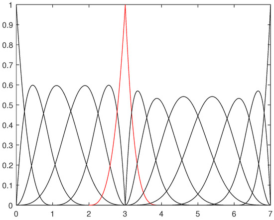
Consider a $C^0$ MD-spline basis with $\mathit{T}:=\left\{0,1,2,3,4,5,6,7\right\}$, $\mathit{G}:=\left\{3,3,3,4,4,\right.$$\left.4,4\right\}$ and $\mathit{K}:=\left\{2,2,0,3,3,3\right\}$. The first function $N_{1,4}$ and the last function $N_{13,4}$ are Bernstein polynomials. Function $N_{6,4}$ is $C^0$ continuous at $t=3$, and it is plotted in red in Figure 2. Other functions are all B-spline functions, where $N_{i,4},i=2,3,4,5$ are $C^2$ functions and $N_{i,4},i=7,...,12$ are $C^3$ functions. In addition, all functions $N_{i,4},i=1,...,13$ define a $C^0$ MD-spline basis. It holds

$$N_{6,4}\left(t\right)=\left((0,0,0,1),(1,0,0,0,0)\right)\left(\begin{array}{c}{b}_{0,3}^2\left(t\right)\\ ⋮\\ b_{3,3}^2\left(t\right)\\ b_{0,4}^3\left(t\right)\\ ⋮\\ b_{4,4}^3\left(t\right)\end{array}\right).$$

(16)

Figure 2. An example of $C^0$ multi-degree spline basis functions.

$N_{6,4}$ is a $C^0$ function, and its Bernstein representation vector on each interval is composed of an entry equal to 1 and the rest are equal to 0, while the Bernstein representation vectors of B-spline functions include several nonzero entries.

3.2. Recursive Process

The recursion of Bernstein representation vectors is determined by Equation (6) and the integral property of Bernstein polynomial [26]. Each vector ${\mathit{A}}_{i,n}^j$ is affected not only by ${\mathit{A}}_{r,n-1}^j,r=i,i+1$, but also by ${\mathit{A}}_{i,n}^r,r=p\left(s_i\right),\dots ,j-1$ and ${\mathit{A}}_{i,n}^r,r=j+1,\dots ,p\left(x_{i-D+n}\right)-1$; hence, the recursive relationship should be evaluated on distinct intervals.

On interval $[t_j,t_{j+1})\subseteq [t_{p\left(s_i\right)},t_{p\left(x_{i+D-n}\right)})$, consider the following $(d_j+n-D+1)\times (d_j+n-D+2)$ matrix

$$\mathit{H}:=\left(\begin{array}{ccccc}0& 1& 1& \cdots & 1\\ 0& 0& 1& \cdots & 1\\ ⋮& ⋮& \ddots & \ddots & ⋮\\ 0& 0& 0& \cdots & 1\end{array}\right).$$

(17)

The integral of Bernstein polynomials satisfy the equality

$$\left(\begin{array}{c}{\int }_{t_j}^t{b}_{0,d_j+n-D}^j\left(y\right)dy\\ ⋮\\ {\int }_{t_j}^t{b}_{d_j+n-D,d_j+n-D}^j\left(y\right)dy\end{array}\right)=\frac{t_{j+1}-t_j}{d_j+n-D+1}\mathit{H}{\mathit{B}}_{d_j+n-D+1}^j\left(t\right),$$

(18)

According to the integral formula, the integral of $N_{i,n}$ is determined as follows:

$${\int }_{t_j}^t{N}_{i,n}\left(y\right)dy={\mathit{A}}_{i,n}^j\frac{t_{j+1}-t_j}{d_j+n-D+1}\mathit{H}{\mathit{B}}_{d_j+n-D+1}^j\left(t\right).$$

(19)

Similarly, another part of the integral is

$${\int }_t^{t_{j+1}}{N}_{i,n}\left(y\right)dy={\mathit{A}}_{i,n}^j\frac{t_{j+1}-t_j}{d_j+n-D+1}\left(\begin{array}{ccccc}1& 0& \cdots & 0& 0\\ 1& 1& \cdots & 0& 0\\ ⋮& \ddots & \ddots & ⋮& ⋮\\ 1& 1& \cdots & 1& 0\end{array}\right){\mathit{B}}_{d_j+n-D+1}^j\left(t\right).$$

(20)

The integral recursion can be substituted by the recursive process of Bernstein representation vectors according to Equation (19). The matrix H is just presented in (18) for simplicity of expression. A cumulative-sum operation can be used to describe the recursion of a representation vector in calculation.

Without loss of generality, assuming that ${\mathit{A}}_{i,n}^j=(a_0,a_1,\dots ,a_{d_j+n-D})$ on interval $[t_j,t_{j+1}),j=p\left(s_i\right),\dots ,p\left(x_{i+n-D}\right)-1$, it holds that

$$N_{i,n}\left(t\right)=(a_0,a_1,\dots ,a_{d_j+n-D}){\mathit{B}}_{d_j+n-D}^j\left(t\right).$$

(21)

We indicates the cumulative-sum operation by an operator $\Gamma$:

$$\Gamma \left({\mathit{A}}_{i,n}^j\right):=\frac{t_{j+1}-t_j}{d_j+n-D+1}(0,a_0,a_0+a_1,\dots ,a_0+a_1+\dots +a_{d_j+n-D}).$$

(22)

Thus,

$${\int }_{t_j}^t{N}_{i,n}\left(y\right)dy=\Gamma \left({\mathit{A}}_{i,n}^j\right){\mathit{B}}_{d_j+n-D+1}^j\left(t\right).$$

(23)

Then, we use an operator $\mathsf{\Lambda }$ to extract the last element of a vector. For example, $\mathsf{\Lambda }\left({\mathit{A}}_{i,n}^j\right)=a_{d_j+n-D}$. Then,

$${\int }_{t_j}^{t_{j+1}}{N}_{i,n}\left(y\right)dy=\mathsf{\Lambda }\left(\Gamma ({\mathit{A}}_{i,n}^j)\right).$$

(24)

Consider $t\in [t_j,t_{j+1}),j=p\left(s_i\right)+1,...,p\left(x_{i+n-D}\right)-1$. The integral starting from $t_{p\left(s_i\right)}$ is

$$\begin{array}{cc}\hfill {\int }_{t_{p\left(s_i\right)}}^t{N}_{i,n}\left(y\right)dy=& \sum _{r=p\left(s_i\right)}^{j-1}\left[\left(\mathsf{\Lambda }\left(\Gamma \left({\mathit{A}}_{i,n}^r\right)\right)\right)\right]+\Gamma \left({\mathit{A}}_{i,n}^j\right){\mathit{B}}_{d_j+n-D+1}^j\left(t\right),\hfill \\ \hfill =& \left[\sum _{r=p\left(s_i\right)}^{j-1}\left[\left(\mathsf{\Lambda }\left(\Gamma \left({\mathit{A}}_{i,n}^r\right)\right)\right)\right]\oplus \Gamma \left({\mathit{A}}_{i,n}^j\right)\right]{\mathit{B}}_{d_j+n-D+1}^j\left(t\right),\hfill \end{array}$$

(25)

where ${\sum }_{r=p\left(s_i\right)}^{j-1}\left[\left(\mathsf{\Lambda }\left(\Gamma \left({\mathit{A}}_{i,n}^r\right)\right)\right)\right]$ is a constant, and $\Gamma \left({\mathit{A}}_{i,n}^j\right)$ is a vector. The symbol ⊕ means that ${\sum }_{r=p\left(s_i\right)}^{j-1}\left[\left(\mathsf{\Lambda }\left(\Gamma \left({\mathit{A}}_{i,n}^r\right)\right)\right)\right]$ is added to each element in $\Gamma \left({\mathit{A}}_{i,n}^j\right)$.

Using the two operators above, ${\delta }_{i,n}$ can be calculated as follows:

$$\frac{1}{{\delta }_{i,n}}={\int }_{-\infty }^{+\infty }{N}_{i,n}\left(y\right)dy=\sum _{r=p\left(s_i\right)}^{p\left(x_{i-D+n}\right)-1}\left[\mathsf{\Lambda }\left(\Gamma \left({\mathit{A}}_{i,n}^r\right)\right)\right].$$

(26)

Consistent with the conventional B-splines, functions in an MD-spline basis can be independently calculated using a recursive method. According to the Bernstein representation, once the vector ${\overrightarrow{\mathcal{A}}}_{i,D}$ is calculated, function $N_{i,D}$ is determined. Consequently, Bernstein representation vectors can replace functions in the recursive process.

The support interval of $N_{i,D}$, $i=1,\dots ,\mathcal{K}$ is $[s_i,x_i)$; therefore, there are $p\left(x_i\right)-p\left(s_i\right)$ intervals in it. Therefore, we establish an initial $(D+1)\times (p\left(x_i\right)-p\left(s_i\right))$ matrix $\mathit{M}$; each entry is 0 and indicates a vector ${\mathit{A}}_{k,0}^j=0,k=i,\dots ,i+D,j=p\left(s_i\right),\dots ,p\left(x_i\right)-1$.

Matrix $\mathit{M}$ has $D+1$ rows, which means that there are $D+1$ corresponding functions on $[s_i,x_i)$ when $n=0$. However, the indexes of these $D+1$ functions may exceed the limit range $[D+1,\mathcal{K}]$. There are two solutions for this. One does not generate rows whose indexes surpass the maximum allowed range. The other one disregards these rows because all of their elements equal 0. In order to make the algorithm more understandable, we employ the second solution. In the recursive process, we use these vectors ${\mathit{A}}_{k,n}^j,n=0,...,D$ to explain the recursion of matrix $\mathit{M}$ in the algorithm.

There are some details in this procedure.

• The operation (line 12) causes vectors ${\mathit{A}}_{i,n}^j$ with the same index j have the same length, hence allowing these vectors can bulid the matrix $\mathit{M}$.
• ${\mathit{M}}_k$ (line 15) indicates the $k-th$ row of the matrix $\mathit{M}$, and ${\left({\delta }_{k,n}\right)}^{-1}={\mathit{A}}_{k,n}^{p\left(x_{k+n-D}\right)-1}$. Thus each row is normalized.
• There are only two cases of subtraction without considering the subtraction of zero rows (line 19 and 21).
• The subtraction is performed in range (lines 20, 22 and 23).

Algorithm 1 only calculates one function in MD-spline basis. If vectors in the initial matrix are changed to be ${\mathit{A}}_{k,0}^j,k=1,\dots ,\mathcal{K}+D,j=p\left(s_1\right),\dots ,p\left(x_{\mathcal{K}}\right)-1$, all basis functions are produced.

The following is an example for Algorithm 1.

Example 2.

Consider a MD-spline basis with $\mathit{T}:=\left\{0,1,4,7,10\right\}$, $\mathit{G}:=\left\{2,3,4,3\right\}$, and $\mathit{K}:=\left\{1,2,3\right\}$. Two extended partition are $\mathit{S}:=\left\{0,0,0,1,1,4,4\right\}$ and $\mathit{X}:=\left\{1,4,7,10,10,10,10\right\}$. We are aming to calculate function $N_{3,4}$. These partitions are shown in Figure 3.

Figure 3. The setting of Example 2, and the support interval of $N_{3,4}$ is plotted in red.

The support interval of $N_{3,4}$ is $[s_3,x_3)=[0,7)$, and $p\left(s_3\right)=0,p\left(x_3\right)=3$. Thus the order of the initial matrix $\mathit{M}$ is $5\times 3$, then

$$\mathit{M}=\left(\begin{array}{ccc}{\mathit{A}}_{3,0}^0& {\mathit{A}}_{3,0}^1& {\mathit{A}}_{3,0}^2\\ {\mathit{A}}_{4,0}^0& {\mathit{A}}_{4,0}^1& {\mathit{A}}_{4,0}^2\\ {\mathit{A}}_{5,0}^0& {\mathit{A}}_{5,0}^1& {\mathit{A}}_{5,0}^2\\ {\mathit{A}}_{6,0}^0& {\mathit{A}}_{6,0}^1& {\mathit{A}}_{6,0}^2\\ {\mathit{A}}_{7,0}^0& {\mathit{A}}_{7,0}^1& {\mathit{A}}_{7,0}^2\end{array}\right)=\left(\begin{array}{ccc}0& 0& 0\\ 0& 0& 0\\ 0& 0& 0\\ 0& 0& 0\\ 0& 0& 0\end{array}\right).$$

(27)

At the beginning of each loop, value 1 is assigned to the vector that satisfies the condition in line 5 in Algorithm 1. Therefore, ${\mathit{A}}_{7,0}^2=1$.

Algorithm 1 Recursive process of Bernstein representation vectors.

Input:$\mathit{T}$, $\mathit{G}$, $\mathit{K}$, i Output:${\overrightarrow{\mathcal{A}}}_{i,D}$ 1: Initial $\mathit{M}=\left({\mathit{A}}_{k,0}^j\right)$, ${\mathit{A}}_{k,0}^j=0,k=i,...,i+D,j=p\left(s_i\right),...,p\left(x_i\right)-1$; 2: for n $\leftarrow 0$ to $D-1$ do 3:     for k $\leftarrow i$ to $i+D-n$ do 4:         for j $\leftarrow p\left(s_k\right)$ to $p\left(x_{k+n-D}\right)-1$ do 5:            if$(d_j==D-n)$then${\mathit{A}}_{k,n}^j\leftarrow 1$ 6:            end if 7:         end for 8:         for j $\leftarrow p\left(s_k\right)$ to $p\left(x_{k+n-D}\right)-1$ do 9:            ${\mathit{A}}_{k,n}^j\leftarrow {\sum }_{k=p\left(s_i\right)}^{j-1}\left(\mathsf{\Lambda }\left(\Gamma \left({\mathit{A}}_{k,n}^r\right)\right)\right)\oplus \Gamma \left({\mathit{A}}_{k,n}^j\right)$ 10:         end for 11:         for j ←$p\left(s_i\right)$ to $p\left(x_i\right)-1$ do 12:            if ($d_j>=0$) and ($\mathsf{\Lambda }({\mathit{A}}_{k,n}^j==0)$) then ${\mathit{A}}_{k,n}^j\leftarrow \Gamma \left({\mathit{A}}_{k,n}^j\right)$ 13:            end if 14:         end for 15:         if$\mathsf{\Lambda }\left({\mathit{A}}_{k,n}^{p\left(x_{k+n-D}\right)-1}\right)\ne 0$then${\mathit{M}}_k\leftarrow {\left(\mathsf{\Lambda }\left({\mathit{A}}_{k,n}^{p\left(x_{k+n-D}\right)-1}\right)\right)}^{-1}{\mathit{M}}_k$ 16:         end if 17:     end for 18:     for k $\leftarrow i$ to $i+D-n-1$ do 19:         if$\mathsf{\Lambda }\left({\mathit{A}}_{k,n}^{p\left(x_{k+n-D}\right)-1}\right)==0$ and $\mathsf{\Lambda }\left({\mathit{A}}_{k+1,n}^{p\left(x_{k+1+n-D}\right)-1}\right)\ne 0$ then 20:            ${\mathit{M}}_k\leftarrow 1-{\mathit{M}}_{k+1}$$(p\left(s_k\right),p\left(x_{k+1+n-D}\right)-1)$ 21:         else if$\mathsf{\Lambda }\left({\mathit{A}}_{k,n}^{p\left(x_{k+n-D}\right)-1}\right)\ne 0$ and $\mathsf{\Lambda }\left({\mathit{A}}_{k+1,n}^{p\left(x_{k+1+n-D}\right)-1}\right)\ne 0$ then 22:            ${\mathit{M}}_k\leftarrow {\mathit{M}}_k-{\mathit{M}}_{k+1}$$(p\left(s_k\right),p\left(x_{k+n-D}\right)-1)$ 23:            ${\mathit{M}}_k\leftarrow 1-{\mathit{M}}_{k+1}$$(p\left(x_{k+n-D}\right),p\left(x_{k+1+n-D}\right)-1)$ 24:         end if 25:     end for 26:     Delete the last row of $\mathit{M}$; 27: end for

Because there is no $C^0$ function when $n=0,1$. In order to be concise, we start the calculation from $n=2$. In this case, it is easy to get $\mathit{M}$:

$$\mathit{M}=\left(\begin{array}{ccc}{\mathit{A}}_{3,2}^0& {\mathit{A}}_{3,2}^1& {\mathit{A}}_{3,2}^2\\ {\mathit{A}}_{4,2}^0& {\mathit{A}}_{4,2}^1& {\mathit{A}}_{4,2}^2\\ {\mathit{A}}_{5,2}^0& {\mathit{A}}_{5,2}^1& {\mathit{A}}_{5,2}^2\end{array}\right)=\left(\begin{array}{ccc}1& (0,0)& (0,0,0)\\ 0& (1,0)& (0,0,0)\\ 0& (0,1)& (1,0,0)\end{array}\right).$$

(28)

In the third row of M, the results of cumulative sum and normalization operations are as follows:

$$\Gamma \left({\mathit{A}}_{5,2}^1\right)=(0,0,\frac{3}{2});\mathsf{\Lambda }(\Gamma \left({\mathit{A}}_{5,2}^1\right))=\frac{3}{2},$$

(29)

and

$$\Gamma \left({\mathit{A}}_{5,2}^2\right)=(0,1,1,1);\mathsf{\Lambda }(\Gamma \left({\mathit{A}}_{5,2}^1\right))\oplus \Gamma \left({\mathit{A}}_{5,2}^2\right)=(\frac{3}{2},\frac{5}{2},\frac{5}{2},\frac{5}{2}).$$

(30)

Thus ${\delta }_{5,2}=\frac{2}{5}$. Note that $\Gamma \left({\mathit{A}}_{5,2}^0\right)=(0,0)$. After normalization, this row changes into

$${\mathit{M}}_3=\left(\begin{array}{ccc}(0,0)& (0,0,\frac{3}{5})& (\frac{3}{5},1,1,1)\end{array}\right).$$

(31)

Similarly, the second row changes into

$${\mathit{M}}_2=\left(\begin{array}{ccc}(0,0)& (0,1,1)& (0,0,0,0)\end{array}\right).$$

(32)

According to the substraction in Algorithm 1, ${\mathit{M}}_2\leftarrow {\mathit{M}}_2-{\mathit{M}}_3$ equals to $(0,1,1)-(0,0,\frac{3}{5})$ on interval $[t_1,t_2)$ and $(1,1,1,1)-(\frac{3}{5},1,1,1)$ on interval $[t_2,t_3)$. After substraction

$${\mathit{M}}_2=\left(\begin{array}{ccc}(0,0)& (0,1,\frac{2}{5})& (\frac{2}{5},0,0,0)\end{array}\right).$$

(33)

${\mathit{M}}_1\leftarrow {\mathit{M}}_1-{\mathit{M}}_2$ can be computed in the same manner. Then, remove the third row and $\mathit{M}$ change into the subsequent one:

$$\mathit{M}=\left(\begin{array}{ccc}{\mathit{A}}_{3,3}^0& {\mathit{A}}_{3,3}^1& {\mathit{A}}_{3,3}^2\\ {\mathit{A}}_{4,3}^0& {\mathit{A}}_{4,3}^1& {\mathit{A}}_{4,3}^2\end{array}\right)=\left(\begin{array}{ccc}(0,1)& (1,0,0)& (0,0,0,0)\\ (0,0)& (0,1,\frac{2}{5})& (\frac{2}{5},0,0,0)\end{array}\right).$$

(34)

By repeating these operations, then the final vector will be

$$\mathit{M}=\left(\begin{array}{ccc}{\mathit{A}}_{3,4}^0& {\mathit{A}}_{3,4}^1& {\mathit{A}}_{3,4}^2\end{array}\right)=\left(\begin{array}{ccc}(0,0,\frac{1}{3})& (\frac{1}{3},1,\frac{7}{17},\frac{3}{17})& (\frac{3}{17},0,0,0,0)\end{array}\right).$$

(35)

Therefore,

$$N_{3,4}\left(t\right)={\overrightarrow{\mathcal{A}}}_{3,4}{\mathbb{B}}_4=\left(\begin{array}{cccc}{\mathit{A}}_{3,4}^0& {\mathit{A}}_{3,4}^1& {\mathit{A}}_{3,4}^2& \mathbf{0}\end{array}\right){\mathbb{B}}_4=\mathit{M}\left(\begin{array}{c}{\mathbf{B}}_2^0\left(t\right)\\ {\mathbf{B}}_3^1\left(t\right)\\ {\mathbf{B}}_4^2\left(t\right)\end{array}\right).$$

(36)

This example can aid comprehension of this section. Although only a portion of the calculation is displayed, the entire recursion is similar. The representation matrix may be calculated directly, and this method is quite intuitive and straightforward to comprehend.

3.3. Algorithm Analysis

The numerical stability of Algorithm 1 is influenced by the floating point operations. There are three types of operations in the algorithm.

1

Cumulative sum operation: the operation in Algorithm 1 (line 9) is composed of addition and multiplication. All elements in the vector are positive and increasing. If the length of an interval is excessively long, the number of bits of elements may vary significantly. This procedure frequently executes this operation, resulting in numerical inaccuracies.

2

Normalized operation: this operation restricts all elements in ${\overrightarrow{\mathcal{A}}}_{i,n}$ to the range $[0,1]$. Since the denominator is the largest number in this vector and all members are positive, this operation will not result in a significant amount of numerical inaccuracy.

3

Subtraction operation: Equation (19) prevents the scenario where two approximate floating point-numbers are subtracted.

The complexity of Algorithm 1 depends on the settings of the sequences $\mathit{T},\mathit{G},\mathit{K}$, so, like reference [20], we only count the number of operations.

At each recursive level in Algorithm 1, there are no more than $\mathcal{K}-D+n$ non-zero rows of each $\mathit{M}$. Therefore, the total number of non-zero rows will not exceed $\mathcal{K}D$ in the whole recursive process.

• Cumulative sum operation: the number of elements in $\mathit{G}$ is $q+1$; thus, the number of this operation will not exceed $\mathcal{K}D(q+1)$.
• Normalized operation: each non-zero row will be normalized, so the maximum number of this operation is $\mathcal{K}D(q+1)$.
• Subtraction operation: similarly, there are $\mathcal{K}D$ subtraction operations, at most.

Thus, the number of operations will not exceed $\mathcal{K}D(2q+3)$, which is used to estimate the numerical complexity of Algorithm 1.

Due to the recursive nature of Algorithm 1, the cyclical calculation of floating-point numbers may lead to error accumulation. Based on the preceding research, the cumulative sum operation is the primary source of mistake. This error can be reduced by a bidirectional algorithm, and Equation (6) is reformed as follows:

$$N_{i,n}\left(t\right)=\left\{\begin{array}{cc}{\delta }_{i,n-1}{\int }_{-\infty }^t{N}_{i,n-1}\left(s\right)ds,\hfill & \hfill t\in [s_i,s_{i+1}),\\ {\delta }_{i,n-1}{\int }_{-\infty }^t{N}_{i,n-1}\left(s\right)ds-{\delta }_{i+1,n-1}{\int }_{-\infty }^t{N}_{i+1,n-1}\left(s\right)ds,\hfill & \hfill t\in [s_{i+1},\xi ),\\ {\delta }_{i+1,n-1}{\int }_t^{+\infty }{N}_{i+1,n-1}\left(s\right)ds-{\delta }_{i,n-1}{\int }_t^{+\infty }{N}_{i,n-1}\left(s\right)ds,\hfill & \hfill t\in [\xi ,x_{i+n-D-1}),\\ {\delta }_{i+1,n-1}{\int }_t^{+\infty }{N}_{i+1,n-1}\left(s\right)ds,\hfill & \hfill t\in [x_{i+n-D-1},x_{i+n-D}),\end{array}\right.$$

(37)

   where $\xi :=s_{i+1}+\lfloor (x_{i+n-D-1}-s_{i+1})/2\rfloor$. The symbol $\lfloor \rfloor$ means rounding down operation.

Then, Algorithm 1 is modified, and the subsequent Algorithm 2 is more numerically stable in calculation.

To represent the reverse integral, we define two reverse operators. Consistent with the prior setting ${\mathit{A}}_{i,n}^j=(a_0,a_1,\dots ,a_{d_j+n-D})$, then $\overline{\Gamma }\left({\mathit{A}}_{i,n}^j\right)=(a_0+\dots +a_{d_j+n-D},a_1+\dots +a_{d_j+n-D},\dots ,a_{d_j+n-D},0)$ and $\overline{\mathsf{\Lambda }}\left({\mathit{A}}_{i,n}^j\right)=a_0$. Algorithm 2 is as follows:

Algorithm 2 Revised recursive method.

1: Same setting as Algorithm 1; 2: for n $\leftarrow 0$ to $D-1$ do 3:     for k $\leftarrow i$ to $i+D-n$ do 4:         for j $\leftarrow p\left(s_k\right)$ to $p\left(x_{k+n-D}\right)-1$ do 5:            if $(d_j==D-n)$then${\mathit{A}}_{k,n}^j\leftarrow 1$ 6:            end if 7:         end for 8:     end for 9:     ${\mathit{M}}^L\leftarrow \mathit{M},{\mathit{M}}^R\leftarrow \mathit{M}$; 10:     for j $\leftarrow p\left(s_k\right)$ to $p\left(x_{k+n-D}\right)-1$ do 11:         ${\mathit{M}}_{k,j}^L\leftarrow {\sum }_{r=p\left(s_i\right)}^{j-1}\left(\mathsf{\Lambda }\left(\Gamma \left({\mathit{A}}_{k,n}^r\right)\right)\right)+\Gamma \left({\mathit{A}}_{k,n}^j\right)$; 12:         ${\mathit{M}}_{k,j}^R\leftarrow {\sum }_{r=j+1}^{p\left(x_{k-D+n}\right)-1}\left(\overline{\mathsf{\Lambda }}\left(\overline{\Gamma }\left({\mathit{A}}_{k,n}^r\right)\right)\right)+\overline{\Gamma }\left({\mathit{A}}_{k,n}^j\right)$; 13:     end for 14:     Extend zero vectors; 15:     if $\mathsf{\Lambda }\left({\mathit{M}}_{k,p\left(x_{k+n-D}\right)-1}^L\right)\ne 0$ then ${\mathit{M}}_k^L\leftarrow {\left(\mathsf{\Lambda }\left({\mathit{M}}_{k,p\left(x_{k+n-D}\right)-1}^L\right)\right)}^{-1}{\mathit{M}}_k^L$ 16:     end if 17:     if $\overline{\mathsf{\Lambda }}\left({\mathit{M}}_{k,p\left(s_k\right)}^R\right)\ne 0$ then ${\mathit{M}}_k^R\leftarrow {\left(\overline{\mathsf{\Lambda }}\left({\mathit{M}}_{k,p\left(s_k\right)}^R\right)\right)}^{-1}{\mathit{M}}_k^R$ 18:     end if 19:     for k $\leftarrow i$ to $i+D-n-1$ do 20:         for j $\leftarrow p\left(s_k\right)$ to $p\left(s_{k+1}\right)$ do 21:            ${\mathit{M}}_{k,j}\leftarrow {\mathit{M}}_{k,j}^L$; 22:         end for 23:         for j $\leftarrow p\left(s_{k+1}\right)$ to $p\left(s_{k+1}\right)+\lfloor (p\left(x_{k+n-D}\right)-1-p\left(s_{k+1}\right))/2\rfloor$ do 24:            ${\mathit{M}}_{k,j}\leftarrow {\mathit{M}}_{k,j}^L-{\mathit{M}}_{k+1,j}^L$; 25:         end for 26:         for j←$p\left(s_{k+1}\right)+\lfloor (p\left(x_{k+n-D}\right)-1-p\left(s_{k+1}\right))/2\rfloor +1$ to $p\left(x_{k+n-D}\right)-1$ do 27:            ${\mathit{M}}_{k,j}\leftarrow {\mathit{M}}_{k+1,j}^R-{\mathit{M}}_{k,j}^R$; 28:         end for 29:         for j $\leftarrow p\left(x_{k+n-D}\right)-1$ to $p\left(x_{k+n-D+1}\right)-1$ do 30:            ${\mathit{M}}_{k,j}={\mathit{M}}_{k+1,j}^R$ 31:         end for 32:     end for 33:     Delete the last row of $\mathit{M}$; 34: end for

3.4. Numerical Experiment

In [20], three typical methods for calculating an MD-spline basis are compared, which are named RKI/Greville, RKI/Derivative and H-Operator. Due to the higher order derivative operations, RKI/Derivative and H-Operator are not numerically stable, while RKI/ Greville avoids these operations and it is numerically stable.

Then, we will design some experiments in Table 1 to test Algorithms 1 and 2. Calculation results are divided into ’Exact’ and ’Numerical’. The ’Exact’ results rely on the symbolic computation in MATLAB, while the ’Numerical’ results are determined by the standard precision in MATLAB (rounding unit $e\approx {10}^{-16}$).

Table 1. Sequences $\mathit{T},\mathit{G},\mathit{K}$ for Tests.

	T	G	K
Test 1	$\left\{0,1,3,7,9,10\right\}$	$\left\{6,5,5,4,5\right\}$	$\left\{5,4,3,4\right\}$
Test 2	$\left\{-{10}^6,-{10}^6+1,0,{10}^6-1,{10}^6\right\}$	$\left\{5,3,3,5\right\}$	$\left\{3,2,3\right\}$
Test 3	$\left\{3^j\right\},j=0,...,12$	$\left\{j\right\},j=10,...,21$	$\left\{j\right\},j=8,...,18$
Test 4	$\left\{2\times j\right\},j=0,...,40$	$\left\{j\right\},j=1,...,40$	$\left\{j\right\},j=0,...,38$

Example 3.

Values in Table 2 are calculated from Algorithm 1, where ’Exact’ in the second column indicates that the Bernstein representation matrix $\mathit{M}$ is calculated through symbolic computation. Exact MD-spline basis and Bernstein basis are also calculated by symbolic computation. The absence of relative error in the third column demonstrates that Algorithm 1 is correct.

Table 2. Algorithm 1 numerical results of Example 3 in Test 1.

t	’Exact’ ${\mathit{N}}_5\left(\mathit{t}\right)$	Relative Error	’Numerical’ ${\mathit{N}}_5\left(\mathit{t}\right)$	Relative Error
2	$1.673419034377224\times {10}^{-1}$	0	$1.673419034377223\times {10}^{-1}$	$3.1616\times {10}^{-16}$
3	$3.951056203260072\times {10}^{-1}$	0	$3.951056203260071\times {10}^{-1}$	$3.0341\times {10}^{-16}$
5	$3.797960943382186\times {10}^{-1}$	0	$3.797960943382184\times {10}^{-1}$	$5.0188\times {10}^{-16}$
7	$5.419134913010994\times {10}^{-2}$	0	$5.419134913010981\times {10}^{-2}$	$2.3148\times {10}^{-15}$

Example 4.

This experiment demonstrates that Algorithm 1 requires revision. The addition of two floating integers with significantly dissimilar digits will result in significant numerical errors. In Table 3, the value produced by Algorithm 1 on the third row has a large relative error and does not symmetric with the first value, whereas the problem is avoided by Algorithm 2.

Table 3. Comparison of Algorithm 1 and Algorithm 2 numerical results in Test 2.

t	Alg 2 ${\mathit{N}}_5\left(\mathit{t}\right)$	Relative Error	Alg 1 ${\mathit{N}}_5\left(\mathit{t}\right)$	Relative Error
−999,999	4.500002750000809 $\times {10}^{-13}$	2.2439 $\times {10}^{-16}$	4.500002750000810 $\times {10}^{-13}$	4.4877 $\times {10}^{-16}$
0	5.000000833333360 $\times {10}^{-1}$	2.2204 $\times {10}^{-16}$	5.000000833333362 $\times {10}^{-1}$	2.2204 $\times {10}^{-16}$
999,999	4.500002750000809 $\times {10}^{-13}$	2.2439 $\times {10}^{-16}$	4.499733918805759 $\times {10}^{-13}$	5.9740 $\times {10}^{-5}$

Example 5.

Table 4 illustrates the values and relative errors of $N_{17,21}$ for Test 3. The RKI/Greville method is unquestionably stable. Algorithm 2 has adequate numerical precision in this instance, where the highest degree exceeds 20. This algorithm is typically stable in experiments below this degree.

Table 4. Comparison of Algorithm 2 and RKI/Greville method numerical results in Test 3.

t	Alg 2 ${\mathit{N}}_{17}\left(\mathit{t}\right)$	Relative Error	RKI/Greville ${\mathit{N}}_{17}\left(\mathit{t}\right)$	Relative Error
27	2.015443122101803 $\times {10}^{-15}$	3.5939 $\times {10}^{-15}$	2.015443122101811 $\times {10}^{-15}$	1.9570 $\times {10}^{-16}$
243	6.858212462569680 $\times {10}^{-4}$	3.1905 $\times {10}^{-15}$	6.858212462569703 $\times {10}^{-4}$	1.5809 $\times {10}^{-16}$
729	1.743353153410859 $\times {10}^{-1}$	7.3071 $\times {10}^{-16}$	1.743353153410862 $\times {10}^{-1}$	6.3683 $\times {10}^{-16}$
2187	3.858286138702032 $\times {10}^{-1}$	3.6662 $\times {10}^{-16}$	3.858286138702034 $\times {10}^{-1}$	8.6325 $\times {10}^{-16}$
6561	2.453976654577640 $\times {10}^{-3}$	3.9579 $\times {10}^{-16}$	2.453976654577639 $\times {10}^{-3}$	1.7672 $\times {10}^{-16}$

Example 6.

This experiment shows that the efficiency of different methods, as measured by MATLAB execution time. Results in Table 4 are calculated using the same point values for four tests. All tests are performed on an environment consisting of MATLAB 2020a and the AMD Ryzen 5 4600U.

Calculating the values of basis functions at the internal knots yields the running time. Note that Algorithm 2 can calculate a single function in the MD-spline basis; its experiment is divided into two separate instances. The information displayed in the second column of Table 4 represents the duration of a single basis function. In order to ensure that values of this function are not zero at most knots, we select the middle basis function. A second scenario involves calculating the values of all basis functions at knots.

Based on the data in Table 5, it is evident that the efficacy of Algorithm 2 is assured. When the degree of basis is low, as in Test 1 and Test 2, there is little difference between the computation times of single functions and whole functions. However, as the degree increases, so does the efficiency gap.

Table 5. Running time in different tests.

Test	Alg 2 (s)	Alg 2 Global (s)	RKI/Greville (s)
Test 1	0.091	0.106	0.117
Test 2	0.088	0.098	0.101
Test 3	0.105	0.254	0.301
Test 4	0.205	1.294	3.070

In some extreme cases, such as Test 4, the degrees of the basis functions are extremely high, making it inefficient to calculate the values of all functions. As the RKI/Greville method is calculated on separate pieces, it needs longer running time.

Compared to the RKI/Greville method, Algorithm 2 is less accurate numerically but more efficient in its calculations. Using a B-spline basis instead of a Bernstein basis as representation functions can improve the numerical precision due to the smaller representation matrix reducing the number of floating-point operations.

Recursive Bernstein representation is not only meaningful for calculation, but it also provides a tool for investigating the recursive relations of MD-spline.

4. Generalized de Boor–Cox-Type Recursive Relations

In this section, we will discuss two generalized de Boor–Cox-type relations of MD-splines.

4.1. The First Form of Generalized de Boor–Cox-Type Relation

A de Boor–Cox-type formula for $C^1$ MD-spline bases exists because $C^0$ functions are formed by two or three Bernstein polynomial segments, and vectors corresponding to $C^0$ functions on each interval are composed of an entry equal to 1 and the rest equal to several elements at 0. Therefore, $C^1$ functions can always be represented by two $C^0$ functions. However, this type of relation does not exist between $C^k$, $k>1$, functions and $C^{k-1}$ functions.

Theorem 1.

There is no de Boor–Cox-type recursive relation for $C^k$ MD-spline basis for $k>1$.

Proof of Theorem 1.

For a $C^k$, $k>1$, function $N_{i,D}$, assume that the following equation holds:

$$N_{i,D}\left(t\right)=f_1\left(t\right)N_{i,D-1}\left(t\right)+f_2\left(t\right)N_{i+1,D-1}\left(t\right)$$

(38)

where $f_1\left(t\right)$ and $f_2\left(t\right)$ are two polynomials of degree 1. Without loss of generality, on a single interval $[t_j,t_{j+1})$, let ${\mathit{A}}_{i,D-1}^j=(a_{11},a_{12},\dots ,a_{1s})$ and ${\mathit{A}}_{i+1,D-1}^j=(a_{21},a_{22},\dots ,a_{2s})$. Both vectors ${\mathit{A}}_{i,D-1}^j$ and ${\mathit{A}}_{i+1,D-1}^j$ contain more than one non-zero element. Using ${\mathit{A}}_{i,D}^j\left(h\right)$ to indicate the h-th element of ${\mathit{A}}_{i,D}^j$, it should be satisfied that

$$\begin{array}{cc}\hfill {\mathit{A}}_{i,D}^j\left(h\right)=& c+\frac{t-t_j}{t_{j+1}-t_j}\sum _{p=1}^h({\delta }_{i,D-1}{a}_{1p}-{\delta }_{i+1,D-1}{a}_{2p})+\frac{t_{j+1}-t}{t_{j+1}-t_j}\sum _{p=1}^{h-1}({\delta }_{i,D-1}{a}_{1p}-{\delta }_{i+1,D-1}{a}_{2p})\hfill \\ \hfill =& C_h+\frac{t-t_j}{t_{j+1}-t_j}({\delta }_{i,D-1}{a}_{1h}-{\delta }_{i+1,D-1}{a}_{2h})\hfill \\ \hfill =& f_1\left(t\right)a_{1h}+f_2\left(t\right)a_{2h},\hfill \end{array}$$

(39)

where c and $C_h$ are two constants. Then, functions $f_1\left(t\right)$ and $f_2\left(t\right)$ will be

$$f_1\left(t\right)=\frac{t-t_j}{t_{j+1}-t_j}{\delta }_{i,D-1}+\alpha ;f_2\left(t\right)=-\frac{t-t_j}{t_{j+1}-t_j}{\delta }_{i+1,D-1}+\beta ;\alpha a_{1h}+\beta a_{2h}=C_h,$$

(40)

where $\alpha$ and $\beta$ are two unknown real numbers. As h is arbitrary, we have

$$\alpha a_{11}+\beta a_{21}=C_1;\dots \alpha a_{1h}+\beta a_{2h}=C_h;\dots \alpha a_{1s}+\beta a_{2s}=C_s.$$

(41)

Since there are more than one non-zero element in ${\mathit{A}}_{i,D-1}^j$ and ${\mathit{A}}_{i+1,D-1}^j$, system (41) is overdetermined and has no solution in most cases. Thus, Equation (38) does not hold.    □

Any $C^k,k>1$, MD-spline basis function can be represented as several $C^0$ functions.

Theorem 2.

For $C^k,k>1$ MD-spline basis, assume that functions ${\left\{N_{i,s}\right\}}_{i=D-s+1}^{\mathcal{K}}$ are all $C^0$ functions or Bernstein polynomials. Then, function $N_{i,n},n>s$, can be represented as

$$N_{i,n}\left(t\right)=f_{i,s}\left(t\right)N_{i,s}\left(t\right)+f_{i+1,s}\left(t\right)N_{i+1,s}\left(t\right)+...+f_{i+n-s,s}\left(t\right)N_{i+n-s,s}\left(t\right).$$

(42)

Proof. 

Proof of Theorem 2 Since each piece of $C^0$ functions equals to Bernstein polynomial, coefficient polynomials ${\left\{f_{j,s}\right\}}_{j=i}^{i+n-s}$ can be determined by Bernstein representation vectors. Since ${\left\{{\mathit{B}}_{d_j+n-D}^j\right\}}_{j=p\left(s_i\right)}^{p\left(x_{i+D-n}\right)-1}$ can be expressed by ${\left\{{\mathit{B}}_{d_j+s-D}^j\right\}}_{j=p\left(s_i\right)}^{p\left(x_{i+D-n}\right)-1}$ as

$${\mathit{B}}_{d_j+n-D}^j={\mathit{L}}_{s,n}^j{\mathit{B}}_{d_j+s-D}^j,$$

(43)

where

$${\mathit{L}}_{s,n}^j=\left(\begin{array}{cc}{b}_{0,n-s}^j\left(t\right)& \\ b_{1,n-s}^j\left(t\right)& b_{0,n-s}^j\left(t\right)& \\ ⋮& ⋮& \ddots \\ b_{n-s,n-s}^j\left(t\right)& b_{n-s,n-s-1}^j\left(t\right)& \ddots & b_{0,n-s}^j\left(t\right)\\ & b_{n-s,n-s}^j\left(t\right)& \ddots & ⋮\\ & & & b_{n-s-1,n-s}^j\left(t\right)\\ & & & b_{n-s,n-s}^j\left(t\right)\end{array}\right),$$

(44)

$N_{i,n}$ can also be expressed by ${\{{\mathit{B}}_{d_j+s-D}^j\}}_{j=p\left(s_i\right)}^{p\left(x_{i+D-n}\right)-1}$. Therefore, Equation (42) always holds in the inner interval $[t_{p\left(s_i\right)+1},t_{p\left(x_{i-D+n}\right)-1})$, and we only need to focus on the first interval $[t_{p\left(s_i\right)},t_{p\left(s_i\right)+1})$ and the last interval $[t_{p\left(x_{i-D+n}\right)-1},t_{p\left(x_{i-D+n}\right)})$.

On the first one $[t_{p\left(s_i\right)},t_{p\left(s_i\right)+1})$, assume that ${\mathit{A}}_{i,s}^{p\left(s_i\right)}\left(j\right)=1$; then, elements from the first to $(j+s-1)$th in ${\mathit{A}}_{i,n}^{p\left(s_i\right)}$ are 0, and ${\mathit{A}}_{i,n}^{p\left(s_i\right)}(j+s)$ is nonzero according to the integral property of Bernstein polynomials. Thus, elements from the first to the $(j-1)$th in ${\mathit{A}}_{i,n}^{p\left(s_i\right)}{\mathit{L}}_{s,n}^{p\left(s_i\right)}$ are 0, which means that ${\mathit{A}}_{i,n}^{p\left(s_i\right)}{\mathit{L}}_{s,n}^{p\left(s_i\right)}={\sum }_{j=i}^{i+n-s}{f}_{j,s}\left(t\right){\mathit{A}}_{j,s}^{p\left(s_i\right)}$.

Similarly, on the last one $[t_{p\left(x_{i-D+n}\right)-1},t_{p\left(x_{i-D+n}\right)})$, this relationship can be determined, then $N_{i,n}$ is expressed as Equation (42).    □

Based on the recursive property of Bernstein polynomials, Theorem 2 reveals a relationship between functions in the recursive process, which is the first form of generalized de Boor–Cox-type relation. The coefficient polynomials ${\left\{f_{j,s}\right\}}_{j=i}^{i+n-s}$ are piecewise, but not unique. Moreover, their domains must fall inside the support intervals of the corresponding functions.

The recursive method of Bernstein representation vectors provides a tool for calculating the coefficient polynomials. Since $C^0$ functions and Bernstein polynomials have unique Bernstein representation vectors, all $\left\{f_{j,s}\right\}{)}_{j=i}^{i+n-s}$ in Equation (42) will be computed from ${\mathit{A}}_{i,n}^j{\mathit{L}}_{s,n}^j$, $j=p\left(s_i\right),...,p\left(x_{i+n-D}\right)-1$.

Note that ${\overrightarrow{\mathcal{A}}}_{j,s},j=i,\dots ,i+n-s$ has a single non-zero element 1 and has the same length as ${\overrightarrow{\mathcal{A}}}_{i,n}$ (line 6) on each interval. Therefore, coefficient $f_{j,s}$ is the corresponding element in ${\overrightarrow{\mathcal{A}}}_{i,n}$, which can be obtained by the element-wise division operation in Algorithm 3 (line 6).

Algorithm 3 Coefficient polynomials calculation.

Input:${\{{\overrightarrow{\mathcal{A}}}_{j,s}\}}_{j=i}^{i+n-s}$ Output:${\{f_{j,s}\}}_{j=i}^{i+n-s}$ 1: Compute ${\overrightarrow{\mathcal{A}}}_{i,n}$ by Algorithm 2 2: for k $\leftarrow p\left(s_i\right)$ to $p\left(x_{i+D}\right)-1$ do 3:     ${\mathit{A}}_{i,n}^k\leftarrow {\mathit{A}}_{i,n}^k{\mathit{L}}_{s,n}^k$; 4: end for 5: for j $\leftarrow i$ to $i+n-s$ do 6:     ${\overrightarrow{\mathcal{A}}}_{j,s}\leftarrow {\overrightarrow{\mathcal{A}}}_{j,s}./{\overrightarrow{\mathcal{A}}}_{i,n}$; 7:     for k $\leftarrow p\left(s_j\right)$ to $p\left(x_{i+s-D}\right)-1$ do 8:         $f_{j,s}^k\left(t\right)\leftarrow {\left({\sum }_{q=1}^{d_k+s-D+1}{\mathit{A}}_{j,s}^k\left(q\right)\right)}^{-1}$; 9:     end for 10: end for

Typically, functions $N_{i,s},N_{i+1,s},\dots ,N_{i+n-s,s}$ are situated at a lower recursive level. Some $C^0$ functions occur at subsequent recursive levels. For instance, $N_{i,s+1}$ is a $C^0$ function and the representation functions of $N_{i,n}$ can be $N_{i,s+1},N_{i+1,s},\dots ,N_{i+n-s,s}$, which are situated at various recursive levels.

Example 7.

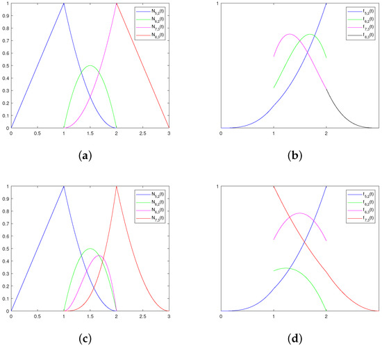
Assume that $\mathit{T}:=\left\{0,1,2,3,5,8\right\}$, $\mathit{G}:=\left\{4,5,4,3,5\right\}$, $\mathit{K}:=\left\{3,2,3,2\right\}$. Then, ${\left\{N_{i,2}\right\}}_{i=5}^8$ are all $C^0$ functions or Bernstein polynomials. Function $N_{5,5}\left(t\right)$ can be represented as follows:

$$N_{5,5}\left(t\right)=f_{5,2}\left(t\right)N_{5,2}\left(t\right)+f_{6,2}\left(t\right)N_{6,2}\left(t\right)+f_{7,2}\left(t\right)N_{7,2}\left(t\right)+f_{8,2}\left(t\right)N_{8,2}\left(t\right),$$

(45)

considering the following diagonally chunked matrix:

$$\mathit{L}=\left(\begin{array}{ccc}{\mathit{L}}_{2,5}^0& & \\ & {\mathit{L}}_{2,5}^1& \\ & & {\mathit{L}}_{2,5}^2\end{array}\right),$$

(46)

where ${\mathit{L}}_{2,5}^0$, ${\mathit{L}}_{2,5}^1$ and ${\mathit{L}}_{2,5}^2$ can be obtained by Equation (44). Then, coefficient polynomials are determined by

$${\mathit{A}}_{5,5}\mathit{L}=\left((0,f_{5,2}^0\left(t\right)),(f_{5,2}^1\left(t\right),f_{6,2}\left(t\right),f_{7,2}\left(t\right)),(f_{8,2}\left(t\right),0)\right).$$

(47)

Next, a distinct set of functions is employed to represent $N_{5,5}$. Note that $N_{7,3}$ is a $C^0$ function, and functions $f_{7,2}$, $f_{8,2}$ in Equation (45) can be replaced by $N_{7,3}$. Over three intervals, the coefficient polynomials must be computed successively. On interval $[2,3)$, it holds that

$${\mathit{A}}_{5,5}^2{\mathit{L}}_{3,5}^2=\left(f_{7,3}^2\left(t\right),0,0\right).$$

(48)

On interval $[1,2)$, it holds that

$${\mathit{A}}_{5,5}^1{\mathit{L}}_{3,5}^1=\left(g_1\left(t\right),g_2\left(t\right),f_{6,3}\left(t\right),f_{7,3}^1\left(t\right)\right),$$

(49)

for the same functions $g_1$ and $g_2$. Then,

$$\left(g_1\left(t\right),g_2\left(t\right),0,0\right){\mathit{L}}_{2,3}^2=\left(f_{5,2}^1\left(t\right),f_{6,2}\left(t\right),0\right).$$

(50)

On interval $[0,1)$, it holds that

$${\mathit{A}}_{5,5}^0{\mathit{L}}_{2,5}^0=\left(0,f_{5,2}^0\left(t\right)\right).$$

(51)

Thus,

$$N_{5,5}\left(t\right)=f_{5,2}\left(t\right)N_{5,2}\left(t\right)+f_{6,2}\left(t\right)N_{6,2}\left(t\right)+f_{6,3}\left(t\right)N_{6,3}\left(t\right)+f_{7,3}\left(t\right)N_{7,3}\left(t\right),$$

(52)

where functions $N_{5,2}$, $N_{6,2}$, $N_{6,3}$, ad $N_{7,3}$ are not at the same level, and the coefficient polynomials $f_{5,2}$ and $f_{6,2}$ are not equivalent to them in Equation (45).

Here, two distinct representations of this function are shown, and Figure 4 depicts the coefficient polynomials. These relationships are prevalent throughout the recursive procedure.

Figure 4. (a) Representation functions $N_{5,2}$, $N_{6,2}$, $N_{7,2}$, $N_{8,2}$. (b) Corresponding coefficient polynomials $f_{5,2}$, $f_{6,2}$, $f_{7,2}$, $f_{8,2}$. (c) Representation functions $N_{5,2}$, $N_{6,2}$, $N_{6,3}$, $N_{7,3}$. (d) Corresponding coefficient polynomials $f_{5,2}$, $f_{6,2}$, $f_{6,3}$, $f_{7,3}$.

Based on the above discussion, functions at the recursive levels n and $n-1$ can all be represented by several $C^0$ functions or Bernstein polynomials. Consequently, $N_{i,n}$ can be represented as follows:

$$N_{i,n}\left(t\right)=f_{i,n-1}\left(t\right)N_{i,n-1}\left(t\right)+f_{i+1,n-1}\left(t\right)N_{i+1,n-1}\left(t\right)+\sum _{j=i}^{i+n-s}{f}_{j,s}\left(t\right)N_{j,s}\left(t\right),$$

(53)

where functions ${\left\{N_{j,s}\right\}}_{j=i}^{i+n-s}$ refer to $C^0$ functions or Bernstein polynomials; $f_{i,n-1}$, $f_{i+1,n-1}$ are polynomials of degree 1. This equation is a general relationship for functions in the MD-spline recursive process.

This subsection summarizes several broad relationships that exist in the recursion; nonetheless, there is no law for generating coefficient polynomials. Consequently, the first generalized de Boor–Cox-type formula lacks practical relevance.

4.2. The Second Form of Generalized de Boor–Cox-Type Relation

Since Equation (38) cannot be found in the recursion of MD-spline basis, we must resort to functions outside of the recursion process in order to obtain this type of formula. If we design two suitable functions that can substitute two functions in the linear combination (42), we have a generalized de Boor–Cox-type formula.

For each $N_{i,n},i=D-n+1,\dots ,\mathcal{K},n=0,\dots ,D$, we have the following result.

Theorem 3.

It holds that

$$N_{i,n}\left(t\right)=(t-t_{p\left(s_i\right)}){\mathcal{L}}_{i,n}\left(t\right)+(t_{p\left(x_{i+n-D}\right)}-t){\mathcal{R}}_{i,n}\left(t\right),$$

(54)

where ${\mathcal{L}}_{i,n}$ and ${\mathcal{R}}_{i,n}$ are both piecewise polynomials.

Proof of Theorem 3.

On interval $[t_j,t_{j+1})\subset [s_i,x_{i+D-n})$, the Taylor expansion of function $N_{i,n}$ is given by all its derivatives. For convenience, let $f\left(t\right)=N_{i,n}\left(t\right),t\in [t_j,t_{j+1})$. Then

$$\begin{array}{cc}\hfill f\left(t\right)=& f\left(t_j\right)+\sum _{r=1}^{d_j+n-D}\frac{1}{r!}{(t-t_j)}^r{f}^{\left(r\right)}\left(t_j\right)\hfill \\ \hfill =& f\left(t_{j+1}\right)+\sum _{r=1}^{d_j+n-D}\frac{1}{r!}{(t_{j+1}-t)}^r{f}^{\left(r\right)}\left(t_{j+1}\right)\hfill \\ \hfill =& f\left(t_j\right)+\sum _{r=1}^{d_j+n-D}\frac{1}{r!}{(t-t_{p\left(s_i\right)}-t_j+t_{p\left(s_i\right)})}^r{f}^{\left(r\right)}\left(t_j\right)\hfill \\ \hfill =& f\left(t_j\right)+\sum _{r=1}^{d_j+n-D}\frac{1}{r!}\left(\sum _{k=0}^r\left(\begin{array}{c}r\hfill \\ k\hfill \end{array}\right){(t-t_{p\left(s_i\right)})}^k{(t_{p\left(s_i\right)}-t_j)}^{r-k}\right)f^{\left(r\right)}\left(t_j\right)\hfill \\ \hfill =& \sum _{r=0}^{d_j+n-D}{(t_{p\left(s_i\right)}-t_j)}^r{f}^{\left(r\right)}\left(t_j\right)\hfill \\ \hfill +& (t-t_{p\left(s_i\right)})\sum _{r=1}^{d_j+n-D}\frac{1}{r!}\left(\sum _{k=0}^{r-1}\left(\begin{array}{c}r\hfill \\ k\hfill \end{array}\right){(t-t_{p\left(s_i\right)})}^k{(t_{p\left(s_i\right)}-t_j)}^{r-1-k}\right)f^{\left(r\right)}\left(t_j\right)\hfill \\ \hfill =& \sum _{r=0}^{d_j+n-D}{(t_{j+1}-t_{p\left(x_{i+n-D}\right)})}^r{f}^{\left(r\right)}\left(t_{j+1}\right)\hfill \\ \hfill +& (t_{p\left(x_{i+n-D}\right)}-t)\sum _{r=1}^{d_j+n-D}\frac{1}{r!}\left(\sum _{k=0}^{r-1}\left(\begin{array}{c}r\hfill \\ k\hfill \end{array}\right){(t_{p\left(x_{i+n-D}\right)}-t)}^k{(t_{j+1}-t_{p\left(x_{i+n-D}\right)})}^{r-1-k}\right)f^{\left(r\right)}\left(t_{j+1}\right).\hfill \end{array}$$

(55)

Let

$$\begin{array}{cc}\hfill {\mathcal{L}}_{i,n}\left(t\right)=& \frac{1}{2}\sum _{r=1}^{d_j+n-D}\frac{1}{r!}\left(\sum _{k=0}^{r-1}\left(\begin{array}{c}r\hfill \\ k\hfill \end{array}\right){(t-t_{p\left(s_i\right)})}^k{(t_{p\left(s_i\right)}-t_j)}^{r-1-k}\right)f^{\left(r\right)}\left(t_j\right)\hfill \\ \hfill +& \frac{1}{2(t_{p\left(x_{i+n-D}\right)}-t_{p\left(s_i\right)})}\sum _{r=0}^{d_j+n-D}\left({(t_{p\left(s_i\right)}-t_j)}^r{f}^{\left(r\right)}\left(t_j\right)+{(t_{j+1}-t_{p\left(x_{i+n-D}\right)})}^r{f}^{\left(r\right)}\left(t_{j+1}\right)\right),\hfill \end{array}$$

(56)

and

$$\begin{array}{cc}\hfill {\mathcal{R}}_{i,n}\left(t\right)=& \frac{1}{2}\sum _{r=1}^{d_j+n-D}\frac{1}{r!}\left(\sum _{k=0}^{r-1}\left(\begin{array}{c}r\hfill \\ k\hfill \end{array}\right){(t_{p\left(x_{i+n-D}\right)}-t)}^k{(t_{j+1}-t_{p\left(x_{i+n-D}\right)})}^{r-1-k}\right)f^{\left(r\right)}\left(t_{j+1}\right)\hfill \\ \hfill +& \frac{1}{2(t_{p\left(x_{i+n-D}\right)}-t_{p\left(s_i\right)})}\sum _{r=0}^{d_j+n-D}\left({(t_{p\left(s_i\right)}-t_j)}^r{f}^{\left(r\right)}\left(t_j\right)+{(t_{j+1}-t_{p\left(x_{i+n-D}\right)})}^r{f}^{\left(r\right)}\left(t_{j+1}\right)\right).\hfill \end{array}$$

(57)

Then, Equation (54) holds. □

Functions ${\mathcal{L}}_{i,n}$ and ${\mathcal{R}}_{i,n}$, here, are constructed by $N_{i,n}^{\left(r\right)}\left(t_j\right)$ and $N_{i,n}^{\left(r\right)}\left(t_{j+1}\right),r=0,\dots ,d_j+n-D$. Due to the integral definition of the MD-spline basis, the values of derivatives at $t_j,t_{j+1}$ can be calculated by the functions in previous recursive levels. The derivative equation is as follows:

$$N_{i,n}^{{}^{\prime }}\left(t\right)={\delta }_{i,n-1}{N}_{i,n-1}\left(t\right)-{\delta }_{i+1,n-1}{N}_{i+1,n-1}\left(t\right).$$

(58)

In addition, the values of $N_{i,n}\left(t_j\right)$ and $N_{i,n}\left(t_{j+1}\right)$ can be calculated by the integral of $N_{i,n-1}$ and $N_{i+1,n-1}$.

Consequently, this form of the formula is conceptually similar to the de Boor–Cox formula. Despite the fact that new functions ${\mathcal{L}}_{i,n}$ and ${\mathcal{R}}_{i,n}$ must be generated, they are all constructed using information from previous functions. Only the intricacy of construction needs to be considered. Taylor expansions are only used for theoretical exposition and cannot be implemented in practice. The coefficient polynomials need only be guaranteed to be polynomials of degree 1; they need not be identical to them in Equation (54). It is even feasible to employ piecewise coefficients to lessen the complexity of construction.

The generalized de Boor–Cox-type formula will employ a generalized pyramid structure, which will be contrasted to the pyramid for B-spline in the accompanying illustration.

Example 8.

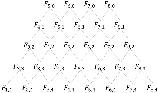
For B-spline basis ${\left\{F_{i,n}\left(t\right)\right\}}_{i=1}^{\mathcal{K}}$, all the basis functions possess similar pyramids; hence, often only one pyramid is depicted. Several pyramids may be utilized to describe the de Boor–Cox recursion for B-splines if the entire basis is used, as shown in Figure 5. The knot sequence is $\mathit{T}:=\left\{0,1,2,3,4\right\}$ and the degree is 4. All pyramids have the same height beginning with the degree 0 functions, i.e., the functions at level 0 in the de Boor–Cox-type recursion.

Figure 5. Pyramids for B-spline basis.

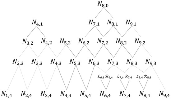
For a MD-spline basis with $\mathit{T}:=\left\{0,1,2,3,4\right\}$, $\mathit{G}:=\left\{3,2,4,3\right\}$, and $\mathit{K}:=\left\{1,1,2\right\}$, the recursive process in Theorem 3 is shown in Figure 6. For a MD-spline basis, pyramids might have varying heights.

Figure 6. Pyramids for MD-spline basis.

Compared with the B-spline basis, the recursive process for the MD-spline basis is determined not only by the degrees but also by the continuous orders.

Although Theorem 3 provides an illustration of the theoretical plausibility of this design, the reality of the building itself is quite complicated. The Bernstein representation approach enables the construction of a structure, but because it is still sophisticated, it is not shown here. If a suitable construction approximation method exists, this theory will be practical.

5. Conclusions

In the paper, we present an evaluation approach for MD-splines. Unlike prior algorithms for evaluating MD-spline bases, this one is non-global, and its intermediate outcomes correspond to functions in the recursive process. Due to the absence of complicated operations, it is efficient in most cases. In addition, its numerical precision in normal degrees is comparable to that of the RKI/Greville approach. In addition to being useful for numerical evaluation, it offers a method for calculating coefficient polynomials in generalized de Boor–Cox-type relations.

Then, we provide two forms of the generalized de Boor–Cox-type formula for MD-splines. Both forms attempt to approximate the de Boor–Cox formula. The first form summarizes the majority of relationships that may appear in the recursion. The second form is a constructed structure. It is theoretically feasible, but requires a computationally cheap building technique.

It is important to note that the present value of the generalized de Boor–Cox-type formula is theoretical, but the preceding numerical algorithm has practical applicability. The second form of the generalized formula has potential because it simply has to address the construction problem. Future work might be devoted to the optimization of the numerical algorithm and the search for better construction techniques.

References

- Carnicer, J.; Peña, J.M. Totally positive bases for shape preserving curve design and optimality of B-splines. Comput. Aided. Geom. Design 1994, 11, 633–654. [Google Scholar] [CrossRef]
- Shen, W.; Wang, G. Changeable degree spline basis functions. J. Comput. Appl. Math. 2010, 234, 2516–2529. [Google Scholar] [CrossRef]
- Nürnberger, G.; Schumaker, L.L.; Sommer, M.; Strauss, H. Generalized Chebyshevian splines. SIAM J. Math. Anal. 1984, 15, 790–804. [Google Scholar] [CrossRef]
- Costantini, P.; Goodman, T.N.T.; Manni, C. Constructing C³ shape-preserving interpolating space curves. Adv. Comput. Math. 2001, 14, 103–127. [Google Scholar] [CrossRef]
- Costantini, P.; Manni, C. Shape-preserving C³ Interpolation: The Curve Case. Adv. Comput. Math. 2003, 18, 41–63. [Google Scholar] [CrossRef]
- Kaklis, P.D.; Pandelis, D.G. Convexity-preserving polynomial splines of non-uniform degree. IMA J. Numer. Anal. 1990, 10, 455–468. [Google Scholar] [CrossRef]
- Costantini, P. Variable degree polynomial splines. In Curves and Surfaces with Applications in CAGD; Vanderbilt University Press: Nashville, TN, USA, 1997; pp. 85–94. [Google Scholar]
- Costantini, P. Curve and surface construction using variable degree polynomial splines. Comput. Aided. Geom. Design 2000, 17, 419–446. [Google Scholar] [CrossRef]
- Sederberg, T.W.; Zheng, J.; Song, X. Knot intervals and multi-degree splines. Comput. Aided. Geom. Design 2003, 20, 455–468. [Google Scholar] [CrossRef]
- Wang, G.Z.; Deng, C.Y. On the degree elevation of B-spline curves and corner cutting. J Comput. Aided. Geom. Design 2007, 24, 90–98. [Google Scholar] [CrossRef]
- Shen, W.; Wang, G. A basis of multi-degree splines. Comput. Aided. Geom. Design 2010, 27, 23–35. [Google Scholar] [CrossRef]
- Shen, W.; Wang, G.; Yin, P. Explicit representations of changeable degree spline basis functions. J. Comput. Appl. Math. 2013, 238, 39–50. [Google Scholar] [CrossRef]
- Shen, W.; Yin, P.; Tang, C. Degree elevation of changeable degree spline. J. Comput. Appl. Math. 2016, 300, 56–67. [Google Scholar] [CrossRef]
- Beccari, C.V.; Casciola, G.; Morigi, S. On multi-degree splines. Comput. Aided. Geom. Design 2017, 58, 8–23. [Google Scholar] [CrossRef]
- Buchwald, B.; Mühlbach, G. Construction of B-splines for generalized spline spaces generated from local ECT-systems. J. Comput. Appl. Math. 2003, 159, 249–267. [Google Scholar] [CrossRef]
- Speleers, H. Algorithm 999: Computation of multidegree B-splines. ACM. Trans. Math. Softw. 2019, 45, 1–15. [Google Scholar] [CrossRef]
- Toshniwal, D.; Speleers, H.; Hiemstra, R.R.; Manni, C.; Hughes, T.J. Multi-degree B-splines: Algorithmic computation and properties. Comput. Aided. Geom. Design 2020, 76, 101792. [Google Scholar] [CrossRef]
- Hiemstra, R.R.; Hughes, T.J.; Manni, C.; Speleers, H.; Toshniwal, D. A Tchebycheffian extension of multi-degree B-splines: Algorithmic computation and properties. SIAM. J. Numer. Anal. 2020, 2, 1138–1163. [Google Scholar] [CrossRef]
- Beccari, C.V.; Casciola, G. Matrix representations for multi-degree B-splines. J. Comput. Appl. Math. 2021, 381, 113007. [Google Scholar] [CrossRef]
- Beccari, C.V.; Casciola, G. Stable numerical evaluation of multi-degree B-splines. J. Comput. Appl. Math. 2022, 400, 113743. [Google Scholar] [CrossRef]
- De Boor, C. On calculating with B-splines. J. Abbr. 1972, 6, 50–62. [Google Scholar] [CrossRef]
- Cox, M. The numerical evaluation of B-splines. J. Inst. Math. Appl. 1972, 10, 134–149. [Google Scholar] [CrossRef]
- Goldman, R. Pyramid Algorithms: A Dynamic Programming Approach to Curves and Surfaces for Geometric Modeling. In The Morgan Kaufmann Series in Computer Graphics; Morgan Kaufmann Publishers, Academic Press: San Diego, CA, USA, 2002; pp. 347–443. [Google Scholar]
- Beccari, C.V.; Casciola, G.A. Cox-de Boor-type recurrence relation for C¹ multi-degree splines. Comput. Aided. Geom. Design 2019, 75, 101784. [Google Scholar] [CrossRef]
- Li, X.; Huang, Z.J.; Liu, Z. A geometric approach for multi-degree spline. J. Comput. Sci. Tech. 2012, 27, 841–850. [Google Scholar] [CrossRef]
- Farouki, R.T. The Bernstein polynomial basis: A centennial retrospective. Comput. Aided. Geom. Design 2012, 29, 379–419. [Google Scholar] [CrossRef]
Disclaimer/Publisher’s Note: The statements, opinions and data contained in all publications are solely those of the individual author(s) and contributor(s) and not of MDPI and/or the editor(s). MDPI and/or the editor(s) disclaim responsibility for any injury to people or property resulting from any ideas, methods, instructions or products referred to in the content. |
© 2023 by the authors. Licensee MDPI, Basel, Switzerland. This article is an open access article distributed under the terms and conditions of the Creative Commons Attribution (CC BY) license (https://creativecommons.org/licenses/by/4.0/).