Abstract
In this paper, we propose an enhanced model for pricing vulnerable options. Specifically, our model assumes that parameters such as interest rates, jump intensity, and asset value volatility are governed by an observable continuous-time finite-state Markov chain. We take into account European vulnerable options that are exposed to both default risk and rare shocks from underlying and counterparty assets. We also consider stochastic default barriers driven by a regime-switching model and geometric Brownian motion, thus improving upon the assumption of fixed default barriers. The risky assets follow a related jump-diffusion process, whereas the default barriers are influenced by a geometric Brownian motion correlated with the risky assets. Within the framework of our model, we derive an explicit pricing formula for European vulnerable options. Furthermore, we conduct numerical simulations to examine the effects of default barriers and other related parameters on option prices. Our findings indicate that stochastic default barriers increase credit risk, resulting in a decrease in option prices. By considering the aforementioned factors, our research contributes to a better understanding of pricing vulnerable options in the context of counterparty credit risk in over-the-counter trading.
MSC:
91G40; 91G80
1. Introduction
The over-the-counter (OTC) market represents a significant portion of the financial market, with many financial institutions actively trading options on it. Unlike exchange-traded markets, OTC transactions are unorganized and lack transparency, which increases the risk of counterparty default. This means that one party may fail to fulfill its contractual obligations. Since the global financial crisis of 2007–2008, participants in the OTC market have become increasingly concerned about the credit default risk associated with options. The structural model, also known as the firm value model, is a key tool for pricing options with credit risk. This article explores option pricing within the framework of the firm value model. Johnson and Stulz [1] were the first to define options with credit risk as vulnerable options.
There are several models for vulnerable option pricing in the literature. Klein [2,3] proposed a model that allows for correlation between the underlying asset of the option and the counterparty’s asset and assumes that the default barrier is the fixed liability of the option writer. He also proposed an improved method that includes both the fixed liabilities of the option writer and losses from vulnerable option shorts in the default barrier. Hui [4] proposed a European vulnerable option pricing model with a stochastic default barrier representing the option writer’s liability. Wang [5] assumed that both the counterparty’s assets and related assets were driven by a related jump-diffusion process and derived a pricing formula for vulnerable options. These studies suggest that the default barrier has an impact on the pricing of European vulnerable options. However, they only consider the impact of barriers on options and do not take into account how a country’s economic status at different times affects option prices.
Since the dynamics of risky asset values are not continuous, some literature introduces jumping processes, compound Poisson processes, or self-exciting Hawkes processes to better describe their value models. These studies discuss the pricing formula for European vulnerable options (see XU [6], TIAN [7], Ma [8], and Zhou [9]). Wang [10] proposed decomposing the underlying asset risk and counterparty assets into systemic and non-systemic risks and used the obtained pricing formula to discuss the difference between vulnerable option prices. In addition, many empirical analyses have concluded that the volatility of risky assets is not fixed. Therefore, some literature assumes that the underlying asset is driven by stochastic volatility models such as the Heston model and mean reversion process and discusses the pricing formula for European vulnerable options (see Liu [11], Yang [12], Lee [13], Wang [14]). Yoon [15] uses double Merlin transforms to obtain closed-form pricing formulas for European vulnerable options under constant and Hull–White interest rate models (see Liu [16]). Huang [17] investigated the pricing of European-style vulnerable options in the presence of non-affine stochastic volatility and double exponential jumps in the underlying asset price process.
Most option pricing models are within the framework of Brownian motion, which makes it difficult to capture external factors such as the state of the national economy. The literature also incorporates vulnerable option pricing under the regime-switching model. Elliott [18,19] was the first to consider introducing regime switching into the option pricing model. Wang [20] uses the local risk minimization method to obtain the optimal hedging strategy for European vulnerable call options. When the option writer’s asset value is depressed by other financial institutions due to poor sales, Yang [21] used polynomial change numerical techniques to obtain a semi-analytical pricing formula for European vulnerable options. Assuming that the default barrier in the vulnerable option model is fixed, Wang [22] assumes that risk assets are driven by regime-switching geometric Brownian motion and obtains a European vulnerable option pricing formula. NIU [23] assumes that the value of risk assets is driven by a relevant regime-switching double exponential jump-diffusion model and uses two-dimensional Laplace transforms to obtain a European vulnerable option pricing formula. Han [24] assumes that the value of risk assets is driven by a relevant regime-switching jump-diffusion model and uses the Esscher transform to select an equivalent martingale measure to obtain a European vulnerable option pricing formula and discusses the impact of jump risk on European vulnerable option pricing. Capponi [25] presents an efficient method for pricing vulnerable contingent claims in a regime-switching market using a suitable change of probability measure and a Poisson series representation. Damircheli [26] investigated the modeling of default probability for publicly traded companies using a synchronous-jump regime-switching model and incorporating tempered stable processes. They proposed an efficient meshfree collocation method to solve the partial integro-differential equations associated with the credit risk model.
However, based on the above literature, we can see that the factors affecting the pricing of European vulnerable options include default barriers, risk asset value models, and national economic conditions. We found that there is currently no study on the pricing of European vulnerable options under a regime-switching model with stochastic default barriers. In light of this, we naturally consider proposing a model that is closer to the actual situation. This article assumes that risky assets are driven by a relevant regime-switching jump-diffusion model and that the default barrier follows a regime-awitching geometric Brownian motion. We obtain an explicit solution for the European vulnerable option pricing formula. In addition, we use numerical simulation to explore the impact of default barriers and parameters on option prices and find that stochastic default barriers increase credit risk, leading to lower option prices. We differ from Han [24] in that they assume that the default barrier is constant. We assume that the dynamics of the default barrier are regime-switching geometric Brownian motions related to the underlying assets and counterparty assets.
The structure of this paper is as follows: Section 2 establishes a regime-switching model for risk assets and default barriers. Section 3 uses the Esscher transform to select an equivalent martingale measure. Section 4 uses the risk-neutral pricing principle to obtain a pricing formula for European vulnerable options. Section 5 presents a numerical analysis of the proposed model using Monte Carlo simulation methods. The conclusion is given in Section 6.
2. Model Description
We construct a continuous-time financial market on a probability space . We assume that all risky assets can be continuously traded in time [0, T]. Let denote a continuous-time Markov process on probability space with a finite state space , where with the -th element is ‘1’. We assume that the states of the economy are modelled by a continuous-time Markov process . According to Elliott [27] semi-martingale decomposition for X, we have , where is Q- matrix of and is a -valued martingale with respect to the natural filtration generated by .
Assumption 1.
The risk-free rate is related to the state of the economy. Let , where . For any , we have ; denotes the inner product of the vector. When ; otherwise, .
Assumption 2.
Suppose that is the market value of the underlying assets at time t, and denote the value of the counterparty’s company assets at time t. and are driven by the following jump-diffusion processes:
For we suppose that denotes the underlying asset’s jump amplitude when the jump happens, following a normal distribution with mean and variance . At any time, and are independent of each other; represents the average jump of the asset. and are the expected return rate of the underlying asset and the volatility of the underlying asset , respectively. and are the expected return rate of the value of the counterparty’s company assets and the volatility of the value of the counterparty’s company assets , respectively. We assume that , , , , , and all depend on the economic state X. Let , , , , , , , where , , , , , , and . For any , and there are .
Assumption 3.
The value of the counterparty’s company liabilities, also called the default barrier, is represented by , and is driven by the following geometric Brownian motion:
Assumption 4.
We assume that the covariance matrix of the Brownian motion on probability space is as follows:
We assume that , , , and are independent of each other. Moreover, we assume that , , , and are independent of . In addition, for the convenience of calculation in the following chapters, we express the relevant three-dimensional Brownian motion , and as
where , and are independent Brownian motions.
Assumption 5.
At the option maturity T, if the value of the counterparty’s company assets is not greater than the value of the counterparty’s company liabilities, we believe that the option has defaulted. The option holder will receive times the notional amount from the option writer, where is the recovery rate. Therefore, at the maturity T, the payment function of the vulnerable European call option with a strike price of is as follows:
3. Selection of Equivalent Martingale Measures
Due to the presence of jumps and the uncertainty introduced by regime switching, the market is incomplete and there are infinitely many equivalent martingale measures. Furthermore, it is not easy to obtain an equivalent martingale measure for two jump-diffusion processes with correlated jumps. It is important to note that while systemic risks can be hedged, non-systematic risks are specific to individual risk assets and cannot be hedged, so their premiums need not be considered. In this paper, we assume that the jump component represents systemic risk and its risk premium must be taken into account. We should measure changes in the jump component. In this section, we apply the regime-switching Esscher transform to select equivalent martingale measures for three stochastic processes with associated jump risks under regime switching.
Using Ito’s theorem, the solutions of Equations (1)–(3) are given by
where is the return process of the underlying asset , is the return process of the underlying asset , and is the return process of the underlying asset . According to the above Equations (7)–(9), we have the three process , and as follows:
Let and be the natural -filtrations generated by and , respectively. For any and , define a filtration such that is the - algebra with . For any , let . Let , , , , , and be the regime-switching Esscher transform parameters, and they are all related to the economic state of . For any , , and , we assume that , , and , where , , and . For the regime-switching Esscher transform parameter , we assume that , where .
Under the given condition , we use the regime-switching Esscher transform proposed by Elliott [18] to select an equivalent martingale measure. Define the equivalent measure of as , the Radon-Nikodym derivative of the regime-switching Esscher transform can be written as follows:
By Equation (5) and calculation, we have
Delbaen [28] showed that the absence of arbitrage is essentially equivalent to the existence of equivalent martingale measures. Under an equivalent martingale measure, the price process of a risky asset is a martingale, which is known as the martingale condition. Due to the uncertainty introduced by the economic state X, the discount process must be defined on a larger filtration R. From the principles of asset pricing and no-arbitrage, it follows that under the equivalent martingale measures , the discount process of risky assets is a martingale.
Theorem 1.
The discounting process of risk assets satisfies the following formula:
if and only if the regime-switching Esscher transform parameters satisfy the following conditions:
where , , , , , , .
Proof.
By Bayes’ rule, we have
So, if and only if the following formula holds, the risk asset discounting process is martingale
Similarly, for the risk asset , the following conditions can be proved:
The following proves the conditions for the equivalent martingale measures of the risk asset . According to Baye’s rule, we also know
We have .
The proof of Theorem 1 is complete. □
Theorem 2.
Under the equivalent martingale measure , , and are driven by the following formula:
where , and are the standard Brownian motion under the equivalent martingale measure , and satisfyes the following relationship:
The covariance matrix of the Brownian motion is the same as that of . , and are Poisson processes with respective intensities , and , respectively. , , and are normal random variables, and , , and . , , and are expressed as the average jumps of , , and , respectively.
Proof.
According to the multi-dimensional Girsanov theorem, under the given conditions and the equivalent martingale measure , we know that and are Brownian motion such that Equations (29)–(31) are established.
Using the theorem T10 [29] (p. 241), we observe that , , and are normal random variables, i.e., , , and . We can calculate , , and .
The proof of Theorem 2 is complete. □
According to Theorem 1, we obtain the martingale condition, but from algebraic knowledge, we know that there are infinite solutions to Equations (18)–(20). In order to facilitate the numerical simulation in Section 5, we provide a set of special solutions. Let
Solving the above equation can obtain the regime-switching Esscher transform parameters as
, , , , , , where , and .
4. Pricing Vulnerable Options
In this section, we derive an explicit formula for pricing vulnerable options. Due to the similarity between call and put options, we only provide detailed calculations for vulnerable European call options.
Theorem 3.
Under the proposed model framework, we obtain the pricing formula of European vulnerable call options as
where is the joint distribution of accumulated stay time given under the equivalent martingale measure . Under the equivalent martingale measure , the characteristic function of satisfies the following formula:
where , , and is a N order diagonal matrix generated by ;
Proof.
According to the principle of risk-neutral pricing, under the equivalent martingale measures , , , and the initial state of the national economy , the European vulnerable options can be written as follows:
where . Under the equivalent martingale measure , the expression of and are expressed by Equations (22)–(24), and the expression of is
The model parameters we propose include the interest rate, jump intensity, and volatility of asset value, which are governed by an observable continuous-time finite-state Markov chain. To facilitate calculations, we need to determine the residence time of each state in the finite-state Markov chain (which can be interpreted as the duration of “good” and “bad” states in the market economy). We assume that represents the staying time of the market economy state in state within [0, T] time, we have
We need to calculate the European call vulnerable options under condition , , and , and first calculate the European call vulnerable option under the given conditions , , , and , i.e.,
In order to calculate the European call vulnerable option under conditions , , and , we need to know the joint conditional distribution of and under the equivalent martingale measure . But and are regulated by the observable continuous-time finite state Markov chain, so the joint conditional distribution of and under the equivalent martingale measure is determined by the conditional joint distribution of the cumulative stay time under conditions , , and under the equivalent martingale measure . Thus, we have
where is the joint distribution of cumulative stay time under the equivalent martingale measure and . Under the equivalent martingale measure , the characteristic function of satisfies the following formula:
where , , and is an N order diagonal matrix generated by . See Buffmgton [26] for proof of theoretical properties.
We next calculate , given the condition and , all jumps are and all jumps are , we have
By calculation, we have
By observing , we find that is a bivariate normal distribution under the equivalent martingale measure . In order to calculate , we first obtain the properties of the bivariate normal distribution as follows:
In order to simplify the calculation, we can rewrite as
where is a two-dimensional standard normal distribution, and the correlation coefficient is . Next, we have
Therefore, given the condition , we can obtain:
The proof of Theorem 3 is complete. □
5. Numerical Simulation
In this section, we present the numerical results of European vulnerable call options prices given by Equations (1)–(3). To facilitate our analysis, we use the set of baseline parameters given in Table 1 and Table 2, and we assume that there are 252 trading days in a year. To facilitate our simulation, we assume that for there are only two regimes, i.e., N = 2. The first regime can be interpreted as a good economic state. The second plan can be interpreted as a bad economic state. We refer to relevant literature (such as Han [24]) to choose the initial state of the economy , and the generation matrix of the Markov chain process

Table 1.
Parameter values of vulnerable European call options in the base case.
Table 2.
Parameter values of vulnerable European call options in the base case.
From Figure 1, it can be observed that as the initial price of the underlying asset, S_0, increases, the price of the European fragile option also increases. This is because as the price of the underlying asset rises, the potential profit for the option holder increases, thereby increasing the value of the option.
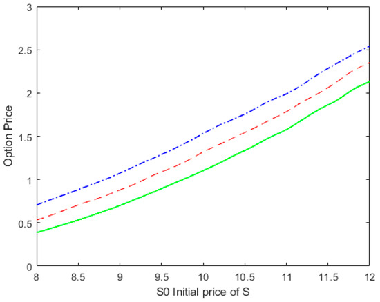
Figure 1.
Vulnerable European call option price against the initial price of the underlying assets S. The solid, dashed, and dot-dashed lines correspond to State 1, the proposed model, and State 2, respectively.
Additionally, we can observe that under State 1 (good economy), the price of the call option is relatively low, whereas under State 2 (bad economy), the price of the call option is relatively high. This is mainly because in a bad economy, the volatility of the risky asset increases, leading to an increase in the risk value of the option. Therefore, investors need to pay a higher price to purchase options under adverse economic conditions.
Furthermore, when considering a mixed state of the economy, i.e., during a transitional period, the value of the option lies between State 1 and State 2. This is because in a mixed state, the economic conditions are uncertain, and the value of the option is influenced by different economic states. As a result, the price of the option falls between the prices observed in a good economy and a bad economy.
In light of these observations, we propose the switching model to better explain the impact of economic conditions on option valuation. In the switching model, the parameters of the risky asset value model evolve under two different economic states, allowing for a more accurate reflection of the changing economic conditions on option values. By introducing the switching model, our model can more flexibly capture changes in economic conditions, thereby better reflecting the pricing of fragile options in practice.
Now, let us turn to Figure 2. Figure 2 shows that as the initial value of the default barrier (counterparty’s debt), D_0, increases, the price of the European fragile option exhibits a decreasing trend. This is because a larger D_0 increases the risk of credit default, reducing the demand for options from investors and leading to a decline in option prices.
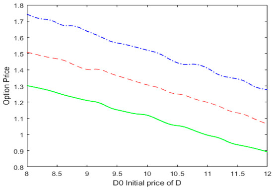
Figure 2.
Vulnerable European call option price against the initial price of the default barrier D. The solid, dashed, and dot-dashed lines correspond to State 1, the proposed model, and State 2, respectively.
Furthermore, by examining Figure 3, we compare the prices of the European fragile option under four different models with the initial price of the underlying asset, S_0. Compared to the Han [24] model, our proposed model has lower prices. This indicates that our model, which considers the dynamic changes in the default barrier, more accurately reflects the increase in default risk, resulting in lower option values. Compared to the Hui [4] model, our model has higher option prices. This is because our model incorporates a jump process of the risky asset, increasing the prices of options and better capturing the impact of economic conditions on options. Compared to the Wang [22] model, when S_0 is between 8 and 9, our model has similar prices to the Wang [22] model. However, when S_0 is between 9 and 12, our model has higher prices.
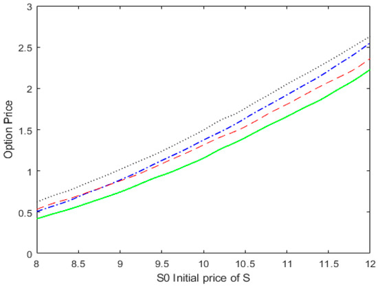
Figure 3.
Vulnerable European call option price against the initial price of the underlying assets S. The solid, dashed, dotted, and dot-dashed lines correspond to Hui’s [4] model, the proposed model, Han’s [22] model, and Wang’s [20] model, respectively.
Figure 4 shows the price of European Vulnerable options plotted against the initial value of the default barrier (D_0) for four different models. As D_0 increases, the price of European Vulnerable options decreases. Notably, our proposed model exhibits lower prices compared to the Han [24] model, indicating that the uncertainty of the default barrier increases over time, resulting in higher default risk and lower option prices. To provide a more comprehensive explanation of these findings, let us delve into the observed models, starting with the Han [24] and Wang [22] models. In these models, as the fixed default barrier (representing the initial value of the counterparty’s liabilities) increases, the option holder assumes higher credit risk. This suggests that if the default barrier is significantly smaller than the counterparty’s assets, the likelihood of default diminishes, leading to higher option prices. Next, let us consider our proposed model and the Hui [4] model. Both models exhibit a similar rate of decline in option prices, indicating that they share a comparable sensitivity to changes in the default barrier. As D_0 increases, the prices of options in both models decline proportionally. Lastly, we compare our proposed model with the Wang [22] model. When D_0 is small, we find that the Wang [22] model yields lower prices compared to our proposed model. This discrepancy arises because, in such instances, the impact of the jump process on credit risk outweighs the effect of the default barrier. These observations provide a detailed explanation of the relationship between the price of European Vulnerable options and the initial value of the default barrier across different models. As D_0 increases, default risk amplifies, leading to a decrease in option prices. Moreover, the influence of the default barrier and the jump process on option prices and credit risk varies among the different models. These findings contribute to a better understanding and assessment of pricing and risk management for vulnerable options.
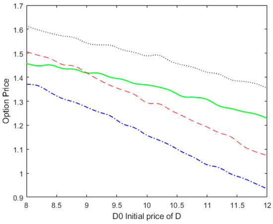
Figure 4.
Vulnerable European call option price against the initial price of the default barrier D. The solid, dashed, dotted, and dot-dashed lines correspond to Wang’s [22] model, the proposed model, Han’s [24] model, and Hui’s [4] model, respectively.
Figure 5, Figure 6, Figure 7 and Figure 8 show the impact of basic parameters on vulnerable option prices, including time to maturity, recovery rate, the correlation coefficient between the underlying asset and the counterparty’s assets, and common jump intensity. These figures display the option prices calculated using our proposed model plotted against the initial price of the underlying asset S_0 from 8 to 12 with alternative basic parameters.
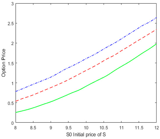
Figure 5.
The option price with different maturity T for , , and . The solid, dashed, and dot-dashed lines correspond to T = 0.5, T = 1, and T = 1.5, respectively.
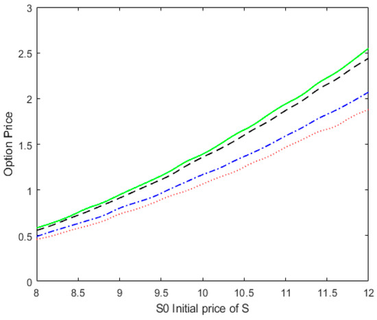
Figure 6.
The option price with different recovery rate for T = 1, , and . The solid, dashed, dotted, and dot-dashed lines correspond to , , , and , respectively.
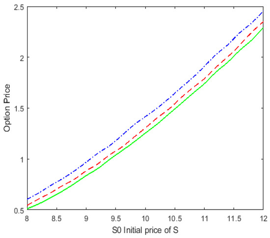
Figure 7.
The option price with a correlation coefficient between the underlying asset and the assets of the counterparty for , , and T = 1. The solid, dashed, and dot-dashed lines correspond to , , and , respectively.
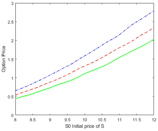
Figure 8.
The option price with different common jump intensity for T = 1, , and . The solid, dashed, and dot-dashed lines correspond to , and , respectively.
As shown in Figure 5, as the option’s time to maturity increases, the option price also increases. This indicates that a longer time to maturity increases the risk of counterparty default and, therefore, increases the value of the option. Figure 6 shows that the option price increases as the recovery rate ω increases. This is because a higher recovery rate results in a higher return at maturity. In Figure 7, we can see that the option price decreases as the correlation coefficient ρ_13 increases. The correlation coefficient reflects the relationship between two assets that move together. This means that as the initial value of the underlying asset S_0 increases, the distance between the three lines also increases. A stronger correlation between the underlying assets and the default barrier means that default risk has a greater impact on vulnerable option prices and results in lower option prices. Figure 8 shows that the option price increases as common jump intensity increases. This result is consistent with our intuitive understanding.
6. Conclusions
This paper discusses the pricing of vulnerable European options using a regime-switching jump-diffusion model. In the structured model, it is assumed that the counterparty’s asset-liability structure (or default barrier) is driven by a geometric Brownian motion under a regime-switching model, and there exists a correlation among all risk assets. By applying the Esscher transform to select an equivalent martingale measure, a pricing formula for vulnerable options is derived. The results of numerical simulations show that the European vulnerable option prices in the proposed model are lower than those in the model assuming a fixed counterparty’s asset–liability structure. This result is intuitive because the counterparty’s liability level is stochastic, increasing the risk of option default and thus lowering the option prices.
This paper mainly investigates the pricing problem of options with random default barriers and credit risk under a regime-switching model. Several research findings are obtained. However, there are still some gaps between the proposed model and the real financial market. Further research can be conducted in the following aspects:
- More data on OTC option trading can be collected to discuss the parameter estimation issues of the relevant pricing models for vulnerable options, referring to existing literature.
- As both models in this paper assume fixed volatility of risk assets and risk-free interest rates, further research directions can consider introducing stochastic volatility and risk-free interest rates into the proposed models to make them adhere to more general models. Additionally, with the advancement of computer performance, alternative methods can be considered to numerically solve the option pricing formulas.
Author Contributions
Methodology, X.L.; Software, Z.Z.; Formal analysis, X.L.; Data curation, Z.Z.; Writing—original draft, Z.Z. All authors have read and agreed to the published version of the manuscript.
Funding
This work was supported by the National Natural Science Foundation of China (No.71471075), Fundamental Research Funds for the Central University (No.19JNLH09), Innovation Team Project in Guangdong Province, P.R. China (No.2016WCXTD004) and Industry -University- Research Innovation Fund of Science and Technology Development Center of Ministry of Education, P.R. China (No.2019J01017).
Data Availability Statement
Not applicable.
Conflicts of Interest
The authors declare that they have no competing interest.
References
- Johnson, H.; Stulz, R. The pricing of options with default risk. J. Financ. 1987, 42, 267–280. [Google Scholar] [CrossRef]
- Klein, P. Pricing Black-Scholes options with correlated credit risk. J. Bank. Financ. 1996, 20, 1211–1229. [Google Scholar] [CrossRef]
- Klein, P.; Inglis, M. Pricing vulnerable European options when the option’s payoff can increase the risk of financial distress. J. Bank. Financ. 2001, 25, 993–1012. [Google Scholar] [CrossRef]
- Hui, C.H.; Lo, C.F.; Ku, K.C. Pricing vulnerable European options with stochastic default barriers. IMA J. Manag. Math. 2007, 18, 315–329. [Google Scholar] [CrossRef]
- Wang, X. Pricing vulnerable options with stochastic default barriers. Financ. Res. Lett. 2016, 19, 305–313. [Google Scholar] [CrossRef]
- Xu, W.; Xu, W.; Li, H.; Xiao, W. A jump-diffusion approach to modelling vulnerable option pricing. Financ. Res. Lett. 2012, 9, 48–56. [Google Scholar] [CrossRef]
- Tian, L.H.; Wang, G.Y.; Wang, X.C. Pricing vulnerable options with correlated credit risk under jump-diffusion processes. J. Futures Mark. 2014, 34, 957–979. [Google Scholar] [CrossRef]
- Ma, Y.; Shrestha, K.; Xu, W. Pricing vulnerable options with jump clustering. J. Futures Mark. 2017, 37, 1155–1178. [Google Scholar] [CrossRef]
- Zhou, Q.; Wang, Q.; Wu, W.X. Pricing vulnerable options with variable default boundary under jump-diffusion processes. Adv. Differ. Equ. 2018, 2018, 465. [Google Scholar] [CrossRef]
- Wang, X. Differences in the prices of vulnerable options with different counterparties. J. Futures Mark. 2017, 37, 148–163. [Google Scholar] [CrossRef]
- Liu, S.I.; Liu, Y.C. Pricing Vulnerable Options under Stochastic Asset and Liability. Prog. Appl. Math. 2011, 1, 12–29. [Google Scholar] [CrossRef]
- Yang, S.J.; Lee, M.K.; Kim, J.H. Pricing vulnerable options under a stochastic volatility model. Appl. Math. Lett. 2014, 34, 7–12. [Google Scholar] [CrossRef]
- Lee, M.K.; Yang, S.J.; Kim, J.H. A closed form solution for vulnerable options with Heston’s stochastic volatility. Chaos Solitons Fractals 2016, 86, 23–27. [Google Scholar] [CrossRef]
- Wang, G.; Wang, X.; Zhou, K. Pricing vulnerable options with stochastic volatility. Phys. A Stat. Mech. Appl. 2017, 485, 91–103. [Google Scholar] [CrossRef]
- Yoon, J.H.; Kim, J.H. The pricing of vulnerable options with double Mellin transforms. J. Math. Anal. Appl. 2015, 422, 838–857. [Google Scholar] [CrossRef]
- Huang, S.; Guo, X. Valuation of European-style vulnerable options under the non-affine stochastic volatility and double exponential jump. Chaos Solitons Fractals 2022, 158, 112003. [Google Scholar] [CrossRef]
- Capponi, A.; Figueroa-López, J.E.; Nisen, J. Pricing and Semimartingale Representations of Vulnerable Contingent Claims in Regime-Switching Markets. Math. Financ. 2014, 24, 250–288. [Google Scholar] [CrossRef]
- Elliott, R.J.; Chan, L.; Siu, T.K. Option pricing and Esscher transform under regime switching. Ann. Financ. 2005, 1, 423–432. [Google Scholar] [CrossRef]
- Elliott, R.J.; Osakwe, C.J.U. Option pricing for pure jump processes with Markov switching compensators. Financ. Stoch. 2006, 10, 250–275. [Google Scholar] [CrossRef]
- Wang, W.; Jin, Z.; Qian, L.; Su, X. Local risk minimization for vulnerable European contingent claims on nontradable assets under regime switching models. Stoch. Anal. Appl. 2016, 34, 662–678. [Google Scholar] [CrossRef]
- Yang, Q.Q.; Ching, W.K.; He, W.; Siu, T.K. Pricing vulnerable options under a Markov-modulated jump-diffusion model with fire sales. J. Ind. Manag. Optim. 2019, 15, 293–318. [Google Scholar] [CrossRef]
- Wang, W.; Wang, W.S. Pricing vulnerable options under a Markov-modulated regime-switching model. Commun. Stat.-Theory Methods 2010, 39, 3421–3433. [Google Scholar] [CrossRef]
- Niu, H.W.; Wang, D.C. Pricing vulnerable options with correlated jump-diffusion processes depending on various states of the economy. Quant. Financ. 2016, 16, 1129–1145. [Google Scholar] [CrossRef]
- Han, M.; Song, X.; Niu, H. Pricing Vulnerable Options with Market Prices of Common Jump Risks under Regime-Switching Models. Discret. Dyn. Nat. Soc. 2018, 2018, 8545841. [Google Scholar] [CrossRef]
- Buffington, J.; Elliott, R.J. Regime switching and European options. In Stochastic Theory and Control-Proceedings of a Workshop held in Lawrence, Kansas, Volume 280 of Lecture Notes in Control and Information Sciences; Springer: Berlin/Heidelberg, Germany, 2002; pp. 73–82. [Google Scholar]
- Damircheli, D.; Razzaghi, M.; Bastani, A.F. A de-singularized meshfree approach to default probability estimation under a regime-switching synchronous-jump tempered stable Lévy model. Eng. Anal. Bound. Elem. 2023, 150, 364–373. [Google Scholar] [CrossRef]
- Elliott, R.J.; Aggoun, L.; Moore, J.B. Hidden Markov Models: Estimation and Control; Springer: New York, NY, USA, 1994. [Google Scholar]
- Delbaen, F.; Schachermayer, W. A general version of the fundamental theorem of asset pricing. Math. Ann. 1994, 300, 463–520. [Google Scholar] [CrossRef]
- Brémaud, P. Point Processes and Queues: Martingale Dynamics; Springer: New York, NY, USA, 1981. [Google Scholar]
Disclaimer/Publisher’s Note: The statements, opinions and data contained in all publications are solely those of the individual author(s) and contributor(s) and not of MDPI and/or the editor(s). MDPI and/or the editor(s) disclaim responsibility for any injury to people or property resulting from any ideas, methods, instructions or products referred to in the content. |
© 2023 by the authors. Licensee MDPI, Basel, Switzerland. This article is an open access article distributed under the terms and conditions of the Creative Commons Attribution (CC BY) license (https://creativecommons.org/licenses/by/4.0/).