New Monotonicity and Infinite Divisibility Properties for the Mittag-Leffler Function and for Stable Distributions

Abstract

Hyperbolic complete monotonicity property ($\mathrm{HCM}$) is a way to check if a distribution is a generalized gamma ($\mathrm{GGC}$), hence is infinitely divisible. In this work, we illustrate to which extent the Mittag-Leffler functions $E_{\alpha },\alpha \in (0,2]$, enjoy the $\mathrm{HCM}$ property, and then intervene deeply in the probabilistic context. We prove that for suitable $\alpha$ and complex numbers z, the real and imaginary part of the functions $x\mapsto E_{\alpha }\left(zx\right)$, are tightly linked to the stable distributions and to the generalized Cauchy kernel.

1. Introduction and First Results

The Mittag-Leffler function,

$$E_a\left(z\right)=\sum _{k\ge 0}\frac{z^k}{\mathsf{\Gamma }(1+ka)},z\in \mathbb{C},a>0,$$

(1)

is a widely studied special function; see [1] and the references therein. The essence of this work is to unveil several probabilistic interpretation for the functions $E_{\alpha },\alpha \in (0,2]$. To this end, we need some setting.

1.1. Bernstein Functions and Infinite Divisibility

A function $f:(0,\infty )\to (0,\infty )$ is completely monotone (we denote $f\in \mathcal{CM}$) if it is infinitely differentiable and it satisfies ${(-1)}^n{f}^{\left(n\right)}\left(x\right)\ge 0,\mathrm{for\; all}n\in \mathbb{N},x>0.$ By Bernstein characterization, $f\in \mathcal{CM}$ if and only if, it is the Laplace transform of some measure

$$f\left(\lambda \right):={\mathfrak{L}}_{\tau }\left(\lambda \right)={\int }_{[0,\infty )}{e}^{-\lambda x}\tau \left(dx\right),\lambda >0.$$

A subset of $\mathcal{CM}$ is the class ${\mathcal{S}}_a$ of generalized Stieltjes transforms of order $a>0$, viz. of functions f represented by

$$f\left(\lambda \right)=\mathrm{d}+\frac{\mathrm{q}}{{\lambda }^a}+{\int }_{(0,\infty )}\frac{1}{{(\lambda +x)}^a}U\left(dx\right),\lambda >0,$$

(2)

where $\mathrm{q},\mathrm{d}\ge 0$ and U is a Radon measure on $(0,\infty )$ such that ${\int }_{(0,\infty )}{(1+u)}^{-a}U\left(du\right)<\infty .$ Stieltjes transforms of order 1 are usually called Stieltjes functions. The class $\mathcal{BF}$ of Bernstein functions consists of functions of the form

$$\begin{array}{ccc}\hfill \varphi \left(\lambda \right)& =& \mathrm{q}+\mathrm{d}\lambda +{\int }_{(0,\infty )}(1-e^{-\lambda x})\Pi \left(dx\right)\hfill \\ & =& \mathrm{q}+\mathrm{d}\lambda +\lambda {\int }_{(0,\infty )}{e}^{-\lambda x}\Pi (x,\infty )dx,\lambda \ge 0,\hfill \end{array}$$

(3)

where $\mathrm{q}\ge 0$ is the so-called killing rate, $\mathrm{d}\in \mathbb{R}$ is the drift, and $\Pi$ is the Lévy measure of $\varphi$, i.e., a positive measure on $(0,\infty )$, which satisfies ${\int }_{(0,\infty )}\left(x\wedge 1\right)\Pi \left(dx\right)<\infty$. Two important subclasses of $\mathcal{BF}$ are the ones of Thorin Bernstein functions and of complete Bernstein functions, denoted by $\mathcal{TBF}$ and $\mathcal{CBF}$, respectively. A function $\varphi$ belongs to $\mathcal{TBF}$ (respectively, $\mathcal{CBF}$) .... if it is represented, for all $\lambda \ge 0,$ by

$$\varphi \left(\lambda \right)=\mathrm{q}+\mathrm{d}\lambda +{\int }_{(0,\infty )}log\left(1+\frac{\lambda }{u}\right)U\left(du\right),\left(\mathrm{resp}.\mathrm{q}+\mathrm{d}\lambda +{\int }_{(0,\infty )}\frac{\lambda }{\lambda +u}V\left(du\right)\right),$$

(4)

where the positive measures U and V satisfy

$${\int }_{(0,1)}|logu|U\left(du\right)+{\int }_{[1,\infty )}{u}^{-1}U\left(du\right)<\infty ,$$

(5)

$\mathrm{and}\frac{V\left(du\right)}{u}\mathrm{is}\mathrm{a}\mathrm{Lévy}\mathrm{measure}.$

Note the equivalences

$$\varphi \in \mathcal{BF}(\mathrm{respectively},\mathcal{TBF},\mathcal{CBF})⟺\varphi \ge 0\mathrm{and}{\varphi }^{\prime }\in \mathcal{CM}(\mathrm{respectively},{\mathcal{S}}_1,{\mathcal{S}}_2).$$

(6)

The book of Hirschman and Widder [2] is a good reference for the classes ${\mathcal{S}}_a$ and, especially for ${\mathcal{S}}_1$, we refer to [3] (Chapter 2). The books of Schilling, Song, and Vondraçek [3] and the one of Steutel and van Harn [4] are our main references for the class $\mathcal{BF}$ and its subclasses, and for infinitely divisible measures as well. The distribution of a nonnegative random variable X is said to be infinitely divisible, and we denote $X\sim \mathrm{I}\mathrm{D}$, if there exists an i.i.d. sequence ${\left(X_i^n\right)}_{1\le i\le n}$, such that $X\stackrel{\mathrm{d}}{=}{X}_1^n+\dots +X_n^n$. The celebrated Lévy-Khintchine formula gives the following characterization through the cumulant function of $X\ge 0$:

$$\begin{array}{ccc}\hfill X\sim \mathrm{I}\mathrm{D}& ⟺& \mathbb{E}{\left[e^{-\lambda X}\right]}^t={\left({\int }_{[0,\infty )}{e}^{-\lambda x}\mathbb{P}(X\in dx)\right)}^t\in \mathcal{CM},\forall t>0\hfill \\ & ⟺& {\varphi }_X\left(\lambda \right):=-log\mathbb{E}\left[e^{-\lambda X}\right]\in \mathcal{BF}.\hfill \end{array}$$

(7)

1.2. The HCM Property and GGC Distributions

The class of infinitely divisible distributions behind $\mathcal{TBF}$ (respectively, $\mathcal{CBF}$) is known as the generalized gamma convolutions $\mathrm{GGC}$ (respectively, the Bondesson class $\mathrm{BO}$), and it corresponds to the smallest class of sub-probability measures on $[0,\infty )$ which contains mixtures of gamma (respectively, exponential) distributions and which is closed under convolutions and vague limits. See [3] (Theorem 9.7 and Proposition 9.11). These classes were introduced by Olaf Thorin, and were widely developed by Lennart Bondesson in [5]; see also [3,4]. We will now introduce an important subclass of $\mathrm{GGC}$. A function $f:(0,+\infty )\to (0,+\infty )$ is said to be hyperbolically completely monotone, and we denote $f\in \mathcal{HCM}$ if, for every $u>0$, the function

$$H_u\left(w\right):=f\left(uv\right)f(u/v),$$

$\mathrm{is}\mathrm{completely}\mathrm{monotone}\mathrm{in}\mathrm{the}\mathrm{variable}w=v+1/v\ge 2,$

(it is easy to see that $H_u$ is always a function of w). In [5] (Theorem 5.3.1), it is shown that the class $\mathcal{HCM}$ corresponds to pointwise limits of functions of the form

$$x\mapsto C{x}^{a-1}\prod _{i=1}^N{(x+c_i)}^{-t_i},N\in \mathbb{N},C,c_i,t_i>0,0<a<\sum _{i=1}^N{c}_i.$$

(8)

Property [5] ((iv) p. 68) asserts that

$$f\in \mathcal{HCM}⟺x^{a}f\left(x^b\right)\in \mathcal{HCM},\mathrm{for}\mathrm{all}a\in \mathbb{R},\mathrm{and}\left|b\right|\le 1.$$

(9)

By Bondessons’s definition [3] (Definition 9.10), and by [3] (Theorem 6.1.1), we have

$$X\sim \mathrm{GGC}⟺{\varphi }_X\in \mathcal{TBF}⟺e^{-{\varphi }_X}\in \mathcal{HCM}.$$

(10)

The class of $\mathcal{HCM}$ functions are stable under multiplicative convolution [5] (property vii, p. 68), then the Laplace transform of an $\mathcal{HCM}$ function is itself $\mathcal{HCM}$. If the p.d.f. of a continuous and positive r.v. X is $\mathcal{HCM}$, we denote $X\sim \mathrm{HCM}$. Clearly, we have the classification

$$\mathrm{HCM}\subset \mathrm{GGC}\subset \mathrm{BO},\mathrm{GGC}\subset \mathrm{SD}\subset \mathrm{I}\mathrm{D},$$

where $\mathrm{SD}$ denotes the well-known class of self-decomposable distributions; see [4] for this class. Note that all previous classes of distributions are stable by additive convolution. The importance of the classes $\mathrm{HCM}$ and $\mathrm{GGC}$ is due to their specific stability properties, one can find in [6]: if X and Y are independent and $X,Y\sim \mathrm{GGC}$ (respectively $\mathrm{HCM}$), then

$$X+Y,X\times Y\sim \mathrm{GGC}(\mathrm{resp}.X^q,q>1,X\times Y,X/Y\sim \mathrm{HCM}).$$

(11)

Note that the above stability properties are not shared by general distribution of the half real line. Moreover, by (7), the $\mathrm{I}\mathrm{D}$ property reads only on the level of the cumulant function, whereas the $\mathrm{HCM}$ one reads on the level of the probability density function, cf. the examples of next subsection. For a better comprehension of the above classes, see Figure 1.

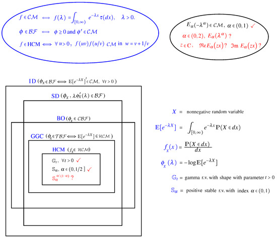
Figure 1. Classes of infinitely divisible distributions, and motivations.

1.3. Gamma and Positive Stable Distributions

In what follows, ${\mathbb{G}}_t$ denotes a standard gamma distributed random variable with shape with parameter $t>0$, i.e., with Laplace transform, Mellin transform, and p.d.f.

$$\begin{array}{ccc}\hfill \mathbb{E}\left[e^{-\lambda {\mathbb{G}}_t}\right]& =& {\left(\frac{1}{1+\lambda }\right)}^t,\lambda \ge 0,\mathbb{E}\left[{\mathbb{G}}_t^s\right]=\frac{\mathsf{\Gamma }(t+s)}{\mathsf{\Gamma }\left(t\right)}s>-t,\hfill \\ \hfill f_{{\mathbb{G}}_t}\left(x\right)& =& \frac{x^{t-1}}{\mathsf{\Gamma }\left(t\right)}{e}^{-x},x>0.\hfill \end{array}$$

(12)

The last p.d.f. form and (8) ensure that all gamma distributions are $\mathrm{HCM}$. Another example of a $\mathrm{GGC}$ distribution is given by the positive stable r.v. ${\mathbb{S}}_{\alpha },\alpha \in (0,1)$, which is associated to the Thorin–Bernstein function

$$\begin{array}{ccc}\hfill {\varphi }_{{\mathbb{S}}_{\alpha }}\left(\lambda \right)& =& -log\mathbb{E}\left[e^{-\lambda {\mathbb{S}}_{\alpha }}\right]=-log{\int }_0^{\infty }{e}^{-\lambda x}{f}_{{\mathbb{S}}_{\alpha }}\left(x\right)dx\hfill \\ & =& {\lambda }^{\alpha }=\frac{\alpha sin\left(\alpha \pi \right)}{\pi }{\int }_0^{\infty }log\left(1+\frac{\lambda }{x}\right)\frac{dx}{x^{1-\alpha }},\lambda \ge 0.\hfill \end{array}$$

(13)

Note that the p.d.f. $f_{{\mathbb{S}}_{\alpha }}$ is not explicit except for $\alpha =1/2$;

$${\mathbb{S}}_{1/2}\stackrel{\mathrm{d}}{=}\frac{1}{4{\mathbb{G}}_{1/2}}\mathrm{and}{f}_{{\mathbb{S}}_{1/2}}\left(x\right)=\frac{1}{2\sqrt{\pi x^3}}{e}^{-1/4x},x>0,$$

(14)

nevertheless, the Mellin transform of ${\mathbb{S}}_{\alpha }$ is explicitly given by

$$\mathbb{E}\left[{\mathbb{S}}_{\alpha }^{-s}\right]=\frac{\mathsf{\Gamma }(1+\frac{s}{\alpha })}{\mathsf{\Gamma }(1+s)},s>-\alpha ,$$

(15)

which gives the convergence in distribution

$$\frac{1}{{\left({\mathbb{S}}_{\alpha }\right)}^{\alpha }}\stackrel{\mathrm{d}}{⟶}1,\mathrm{as}\alpha \to 1,\mathrm{and}\frac{1}{{\left({\mathbb{S}}_{\alpha }\right)}^{\alpha }}\stackrel{\mathrm{d}}{⟶}{\mathbb{G}}_1,\mathrm{as}\alpha \to 0.$$

(16)

It is then natural to adopt the conventions ${\mathbb{S}}_0=0,{\mathbb{S}}_1$. Related literature for the stable distribution is referenced on Nolan’s website [7]. The monograph of Zolotarev [8] is one of the major references for general stable distributions. By representation (13), and by the main result of [9], we know that

$${\mathbb{S}}_{\alpha }\sim \mathrm{GGC},\mathrm{for}\mathrm{all}\alpha \in (0,1),\mathrm{and}{\mathbb{S}}_{\alpha }\sim \mathrm{HCM}⟺\alpha \le 1/2.$$

(17)

Additionally, in [10], it was shown that if $t>0$, then

$${\mathbb{S}}^{-\frac{\alpha }{t}}\sim \mathrm{I}\mathrm{D}⟺t\le 1-\alpha .$$

(18)

Using (16), and taking ${\mathbb{S}}_{\alpha }^{\prime }$ an independent version of ${\mathbb{S}}_{\alpha }$, let us define the quotient,

$${\mathbb{T}}_{\alpha }:={\left(\frac{{\mathbb{S}}_{\alpha }}{{\mathbb{S}}_{\alpha }^{\prime }}\right)}^{\alpha },\alpha \in (0,1),{\mathbb{T}}_1=1,\mathrm{and}{\mathbb{T}}_0\stackrel{\mathrm{d}}{=}\frac{{\mathbb{G}}_1}{{\mathbb{G}}_1^{\prime }},$$

(19)

where ${\mathbb{G}}_1,{\mathbb{G}}_1^{\prime }$ are i.i.d. and standard exponentially distributed. The p.d.f. of ${\mathbb{T}}_{\alpha }$ is explicitly given by the generalized Cauchy form

$$f_{{\mathbb{T}}_{\alpha }}\left(x\right)=\frac{sin\left(\pi \alpha \right)}{\pi \alpha }\frac{1}{1+2cos\left(\pi \alpha \right)x+x^2},x>0,$$

(20)

see (75) below for instance. Bosch [11] completed (18) by showing

$$\alpha \in (0,1/2]\mathrm{and}\left|t\right|\le 1-\alpha ⟺{\mathbb{T}}_{\alpha }^{1/t}={\left(\frac{{\mathbb{S}}_{\alpha }^{\prime }}{{\mathbb{S}}_{\alpha }}\right)}^{\alpha /t}\sim \mathrm{HCM}.$$

(21)

With the above information, Bosch and Simon found it natural to raise the following open question in [9]:

$${\mathbb{S}}_{\alpha }^{\alpha /(1-\alpha )}\sim \mathrm{HCM}⟺{\mathbb{S}}_{\alpha }^{-\alpha /t}\sim \mathrm{HCM} \mathit{if}, \mathit{and} \mathit{only} \mathit{if}, \alpha \le \mathit{1}/\mathit{2} \mathit{and} \left|t\right|\le 1-\alpha ?$$

(22)

This open question extends Bondesson’s conjecture [5], which was stated in 1977. This conjecture, which is identical to (22) with $t=\alpha$, was investigated in [10] and solved in [9].

1.4. First Results on the Mittag-Leffler Functions

From (15), one obtains a first link of the Mittag-Leffler function with the positive stable distribution:

$$\mathbb{E}\left[e^{z/{\left({\mathbb{S}}_{\alpha }\right)}^{\alpha }}\right]=E_{\alpha }\left(z\right),\alpha \in (0,1),z\in \mathbb{C}.$$

(23)

By (13), it is clear that

$$\mathbb{E}\left[e^{-\lambda {\mathbb{T}}_{\alpha }^{1/\alpha }}\right]=\mathbb{E}\left[e^{-\lambda {\mathbb{S}}_{\alpha }^{\prime }/{\mathbb{S}}_{\alpha }}\right]=\mathbb{E}\left[e^{-{(\lambda /{\mathbb{S}}_{\alpha })}^{\alpha }}\right]=E_{\alpha }(-{\lambda }^{\alpha }),\lambda \ge 0.$$

(24)

In [10], if was shown that

$$0<\alpha \le \frac{1}{2}⟺{\mathbb{T}}_{\alpha }^{1/\alpha }\sim \mathrm{HCM}⟹E_{\alpha }(-{\lambda }^{\alpha })\in \mathcal{HCM}.$$

Note that the r.v.

$${\mathbb{R}}_{\alpha }:=1+{\mathbb{T}}_{|\alpha -1|}^{1/\alpha },\alpha \in [0,2],$$

(25)

appeared in [12] ((184) and (223)), in a $\mathrm{GGC}$ context without noticing its $\mathrm{GGC}$ property: by (21), we have

$$\frac{1}{2}\le \alpha \le 1⟺{\mathbb{T}}_{|\alpha -1|}^{1/\alpha }={\mathbb{R}}_{\alpha }-1\sim \mathrm{HCM}⟹{\mathbb{R}}_{\alpha }\sim \mathrm{GGC}.$$

(26)

Another monotonicity property of the Mittag-Leffler functions can be found in [13]:

$$0<\alpha \le \frac{1}{2}⟺\lambda E_{\alpha }(-\lambda )\in \mathcal{BF}⟺1-\mathsf{\Gamma }(1-\alpha )\lambda E_{\alpha }(-\lambda )\in \mathcal{CM},$$

and results in case $\alpha \in (1/2,1)$ are also shown there. Note that the function $E_{\alpha }(-\lambda )$ is completely monotone, contrary to $E_{\alpha }\left(\lambda \right)$. In [14] (Theorem 1.2, (a) and (c)), Simon showed that

$$\lambda \mapsto F_{\alpha }\left(\lambda \right):=\frac{e^{\lambda }-\alpha E_{\alpha }\left({\lambda }^{\alpha }\right)}{1-\alpha }\in \mathcal{CM},\mathrm{for}\mathrm{all}\alpha \in (0,1)\cup (1,2].$$

(27)

The choice of the function $F_{\alpha }$ is intuitive because $e^{\lambda }=E_1\left(\lambda \right)={lim}_{\alpha \to 1}\alpha E_{\alpha }\left({\lambda }^{\alpha }\right)$.

The main objective of this work is to exhibit new monotonicity properties of the $\mathrm{GGC}$ and $\mathrm{HCM}$ type for the Mittag-Leffler functions. To give a taste of our results, we start by improving Simon’s results (27).

Theorem 1.

For $\alpha \in (0,1)\cup (1,2]$, the following holds.

(1) 

With ${\mathbb{T}}_{|\alpha -1|}$ given by (19), and $F_{\alpha }$ by (27), we have the Laplace representation:

$$F_{\alpha }\left(\lambda \right):=\mathbb{E}\left[e^{-\lambda {{\mathbb{T}}_{|\alpha -1|}}^{1/\alpha }}\right],\lambda \ge 0.$$

(28)

(2) 

Assume $\alpha \in (0,1)$.

(a) 

The functions $1-\alpha e^{-\lambda }{E}_{\alpha }\left({\lambda }^{\alpha }\right)$ and $e^{\lambda }/E_{\alpha }\left({\lambda }^{\alpha }\right)$ are completely monotone, and $e^{-\lambda }{E}_{\alpha }\left({\lambda }^{\alpha }\right)-1$ is Bernstein.

(b) 

The function $F_{\alpha }$ is Stieltjes. Moreover, $F_{\alpha }\in \mathcal{HCM}$, if and only if, $1/2\le \alpha <1$. In this case, $1-\alpha e^{-\lambda }{E}_{\alpha }\left({\lambda }^{\alpha }\right)\in \mathcal{HCM}$ and $-F_{\alpha }^{\prime }/F_{\alpha }\in {\mathcal{S}}_1$.

(3) 

Assume $\alpha \in (1,2]$.

(a) 

The function $\alpha e^{-\lambda }{E}_{\alpha }\left({\lambda }^{\alpha }\right)-1$ is completely monotone and $1-e^{-\lambda }{E}_{\alpha }\left({\lambda }^{\alpha }\right)$ is Bernstein.

(b) 

The function $F_{\alpha }$ is not $\mathcal{HCM}$ if $\alpha >4/3$.

(c) 

If $1<\alpha \le 3/2$ and $0<\gamma \le (2-\alpha )/\alpha$, then $F_{\alpha }\left({\lambda }^{\gamma }\right)$ is $\mathcal{HCM}$, and both functions $F_{\alpha }\left({\lambda }^{\gamma }\right)$ and $-{\lambda }^{\gamma -1}{F}_{\alpha }^{\prime }\left({\lambda }^{\gamma }\right)/F_{\alpha }\left({\lambda }^{\gamma }\right)$ are in ${\mathcal{S}}_1$.

In the same direction as (27), Simon considered in [14,15] the function

$$G_{\alpha }\left(x\right):=E_{\alpha }\left(x^{\alpha }\right)-\frac{d}{dx}\left(E_{\alpha }\left(x^{\alpha }\right)\right)=\frac{1-\alpha }{\alpha }\left(F_{\alpha }^{\prime }\left(x\right)-F_{\alpha }\left(x\right)\right),x>0.$$

(29)

From (25) and (28), we deduce the expressions

$$G_{\alpha }\left(x\right)=\frac{\alpha -1}{\alpha }\mathbb{E}\left[\left(1+{\mathbb{T}}_{|\alpha -1|}^{1/\alpha }\right)e^{-x{\mathbb{T}}_{|\alpha -1|}^{1/\alpha }}\right],\alpha \in (0,1)\cup (1,2].$$

(30)

and

$$\frac{\alpha }{\alpha -1}{e}^{-x}{G}_{\alpha }\left(x\right)=\mathbb{E}\left[{\mathbb{R}}_{\alpha }{e}^{-x{\mathbb{R}}_{\alpha }}\right]$$

(31)

$\mathrm{is}\mathrm{the}\mathrm{p.d.f.}\mathrm{of}\mathrm{the}\mathrm{independent}\mathrm{quotient}{\mathbb{G}}_1/{\mathbb{R}}_{\alpha }.$

Using (15), we see that

$$\alpha \in (1,2]⟹\mathbb{E}\left[{\mathbb{T}}_{\alpha -1}^{1/\alpha }\right]=\frac{1}{\alpha -1},$$

(32)

thus

$$⟹G_{\alpha }(0+)=\frac{\alpha -1}{\alpha }\mathbb{E}\left[1+{\mathbb{T}}_{\alpha -1}^{1/\alpha }\right]=1={\int }_0^{\infty }{G}_{\alpha }\left(x\right)dx,$$

which means that $G_{\alpha },\alpha \in (1,2],$ is a p.d.f. and is also the Laplace transform of a probability distribution; see (69) below. In case $\alpha \in (0,1)$, we have $\mathbb{E}\left[{\mathbb{T}}_{1-\alpha }^{1/\alpha }\right]=\infty$, and the function $-G_{\alpha }$ is not a p.d.f. We complete our previous discussion with the following result.

Theorem 2. 

The r.v. ${\mathbb{R}}_{\alpha }$ and the function $G_{\alpha }$, given in (29) and (25), satisfy the following.

(1) 

If $\alpha \in (1,2]$, then the p.d.f. $G_{\alpha }$ is the one of a $\mathrm{GGC}$ distribution but not a $\mathrm{HCM}$.

(2) 

If $\alpha \in (0,1)$, then the function $-G_{\alpha }$ is a widened $\mathrm{GGC}$, if and only if, $\alpha \ge 1/2$. In this case, ${\mathbb{G}}_1/{\mathbb{R}}_{\alpha }\sim \mathrm{GGC}$.

In [16], Simon was interested in the first passage time of the normalized spectrally positive $\alpha$-stable Lévy process ${\left(S_t^{\left(\alpha \right)}\right)}_{t\ge 0},\alpha \in (1,2]$, viz.

$$\mathbb{E}\left[e^{-\lambda S_t^{\left(\alpha \right)}}\right]=e^{t{\lambda }^{\alpha }},\lambda ,t\ge 0,$$

and

$${\widehat{\tau }}_x=inf\{t>0;S_t^{\left(\alpha \right)}=-x\}\mathrm{and}{\tau }_x=inf\{t>0;S_t^{\left(\alpha \right)}=x\},x>0.$$

(33)

The self-similarity property of ${\left(S_t^{\left(\alpha \right)}\right)}_{t\ge 0}$ with index $1=1/\alpha$ entails

$$S_t^{\left(\alpha \right)}\stackrel{\mathrm{d}}{=}{t}^{1/\alpha }{S}_1^{\left(\alpha \right)},({\widehat{\tau }}_x,{\tau }_x)\stackrel{\mathrm{d}}{=}{x}^{\alpha }({\widehat{\tau }}_1,{\tau }_1).$$

Additionally, it is well known that

$${\widehat{\tau }}_1\stackrel{\mathrm{d}}{=}inf\{t>0;S_t^{\left(\alpha \right)}>1\}\stackrel{\mathrm{d}}{=}{\mathbb{S}}_{1/\alpha },$$

and this explains our focus on ${\tau }_1$. To formalize our next results, we need to recall the biasing procedure for the distribution of a non-negative r.v. Z. For $u\in \mathbb{R}$ such that $\mathbb{E}\left[Z^u\right]<\infty$, we denote by $Z^{\left[u\right]}$ a version of the length-biased distribution of order u of Z, viz.

$$\mathbb{P}(Z^{\left[u\right]}\in dx)\stackrel{\mathrm{d}}{=}\frac{x^u}{\mathbb{E}\left[Z^u\right]}\mathbb{P}(Z\in dx).$$

(34)

We complete Simon’s main result in [16] by explaining (in (37) below) his factorization of ${\tau }_1$ obtained in his main theorem, and by the use of the function

$$H_{\alpha }\left(\lambda \right):=(1-\alpha )F_{\alpha }^{\prime }\left({\lambda }^{1/\alpha }\right)=e^{{\lambda }^{\frac{1}{\alpha }}}-{\alpha }^2{\lambda }^{1-\frac{1}{\alpha }}{E}_{\alpha }^{\prime }\left(\lambda \right),\alpha \in (1,2].$$

(35)

Corollary 1.

Let $\alpha \in (1,2]$. The r.v. ${\tau }_1$ given by (33), and $H_{\alpha }$ by (35), satisfy the following.

(1) 

We have the Laplace representation:

$$\mathbb{E}\left[e^{-\lambda {\tau }_1}\right]=H_{\alpha }\left(\lambda \right),\lambda \ge 0.$$

(36)

(2) 

With the convention (19), we have the independent factorizations in law:

$${\tau }_1\stackrel{\mathrm{d}}{=}{\mathbb{S}}_{1/\alpha }{\left({\mathbb{T}}_{\alpha -1}\right)}^{[1/\alpha ]}and{\left(\frac{{\mathbb{G}}_1}{{\tau }_1}\right)}^{1/\alpha }\stackrel{\mathrm{d}}{=}{\mathbb{G}}_1{\left({\mathbb{T}}_{\alpha -1}^{1/\alpha }\right)}^{\left[1\right]},$$

(37)

where the distributions of ${\left({\mathbb{T}}_{\alpha -1}\right)}^{[1/\alpha ]}$ and ${\left({\mathbb{T}}_{\alpha -1}^{1/\alpha }\right)}^{\left[1\right]}$ are given by the biasing procedure (34).

(3) 

${({\mathbb{G}}_1/{\tau }_1)}^{1/(2-\alpha )}\sim \mathrm{HCM}$.

(4) 

If $\alpha \le 3/2$, then ${\tau }_1\sim \mathrm{GGC}$, hence $H_{\alpha }\in \mathcal{HCM}.$

In addition to the above results, which are a continuation of Simon’s ones [14,15,16], we obtain the following ones that we divide, for sake of coherence, into Section 2 and Section 3:

• Proposition 1 is a key to illustrate several other links between the r.v.s ${\mathbb{T}}_{\alpha }$ (19), and the Mittag-Leffler functions;
• A consequence of Proposition 1 is Corollary 3, which builds a new class of $\mathcal{HCM}$ functions, similar to the shapes (8) and (20);
• In Corollary 2 (and also in Theorem 3), we obtain that for any complex number z in the first quadrant, and for $0<t\le 1-argz$, the real and imaginary part of $\lambda \mapsto E_t\left(-z{\lambda }^t\right)$ also enjoy $\mathcal{CM}$, $\mathrm{GGC}$ and $\mathrm{HCM}$ properties;
• With the help of Proposition 1, we characterize in Theorem 3 the distributions of a peculiar family of distributions, which might be helpful in solving the open question (22);
• We conclude with Corollary 4, which provides more information than

To the best of our knowledge, the results of Section 2 and Section 3 have not been addressed in the literature in a form even close to ours, and they constitute a contribution to infinite divisibility, especially in the Bondesson’s $\mathrm{HCM}$ and Mittag-Leffler contexts.

In Section 4, we give comments and perspectives on some of the above results and also settle a prerequisite on the positive stable distributions on the Bernstein functions. The proofs are postponed to Section 5.

2. A New Class of HCM Distributions and $\mathcal{CM}$ Property for $\mathbf{\lambda }\mapsto \mathfrak{Re}\left({\mathbf{E}}_{\mathbf{t}}(-\mathbf{z}{\mathbf{\lambda }}^{\mathbf{t}})\right),\mathbf{z}\in \mathbb{C}$

2.1. The Biasing and the Gamma-Mixture Procedure

Clearly,

$$\mathbb{E}\left[{\left(Z^{\left[u\right]}\right)}^{\lambda }\right]=\frac{\mathbb{E}\left[Z^{\lambda +u}\right]}{\mathbb{E}\left[Z^u\right]}\mathrm{and}{\left(Z^v\right)}^{\left[u\right]}\stackrel{\mathrm{d}}{=}{\left(Z^{\left[uv\right]}\right)}^v,\mathrm{if}\mathbb{E}\left[Z^{uv}\right]<\infty .$$

(38)

A useful result is the stochastic interpretation of property (9):

$$Z\sim \mathrm{HCM}⟺{\left(Z^q\right)}^{\left[u\right]}\stackrel{\mathrm{d}}{=}{\left(Z^{\left[qu\right]}\right)}^q\sim \mathrm{HCM},\mathrm{for}\left|q\right|\ge 1\mathrm{and}\mathrm{all}u\mathrm{s.t.}\mathbb{E}\left[Z^{uq}\right]<\infty .$$

(39)

A random variable ${\mathbb{B}}_{a,b},a,b>0$ has the beta distribution if it has the p.d.f.

$$\frac{\mathsf{\Gamma }(a+b)}{\mathsf{\Gamma }\left(a\right)\mathsf{\Gamma }\left(b\right)}{x}^{a-1}{(1-x)}^{b-1},0<x<1.$$

Observe that ${\mathbb{G}}_t^{\left[u\right]}\stackrel{\mathrm{d}}{=}{\mathbb{G}}_{t+u}$ and ${\mathbb{B}}_{a,b}^{\left[v\right]}\stackrel{\mathrm{d}}{=}{\mathbb{B}}_{a+v,b}$, if $u>-t$ and $v>-a$. By the beta-gamma algebra, we know that if ${\mathbb{B}}_{a,b}$ and ${\mathbb{G}}_{a+b}$ are independent, then

$$({\mathbb{B}}_{a,b},{\mathbb{G}}_{a+b})\stackrel{\mathrm{d}}{=}\left(\frac{{\mathbb{G}}_u}{{\mathbb{G}}_a+{\mathbb{G}}_b},{\mathbb{G}}_a+{\mathbb{G}}_b\right),$$

(40)

$\mathrm{where}{\mathbb{G}}_a\mathrm{and}{\mathbb{G}}_b\mathrm{are}\mathrm{independent}$.

The following fact will be used in the sequel to exhibit several factorizations in law. A positive r.v. X has p.d.f. of the form

$$f_X\left(x\right)=x^{t-1}g\left(x\right),t>0\mathrm{and}g\in \mathcal{CM},$$

(41)

if and only if, the distribution of X is a gamma-mixture of order t (shortly X is a ${\mathbb{G}}_t$-mixture). The latter is equivalent to the existence of a positive r.v. Y such that we have the independent factorization

$$X\stackrel{\mathrm{d}}{=}\frac{{\mathbb{G}}_t}{Y},$$

(42)

and in (42), necessarily

$$g\left(x\right)=\frac{1}{\mathsf{\Gamma }\left(t\right)}\mathbb{E}\left[Y^t{e}^{-xY}\right]\left(=\frac{\mathbb{E}\left[Y^t\right]}{\mathsf{\Gamma }\left(t\right)}\mathbb{E}\left[e^{-x{Y}^{\left[t\right]}}\right],\mathrm{if}\mathbb{E}\left[Y^t\right]<\infty \right).$$

An important result due to Kristiansen [17] asserts that

$$X\mathit{has}\mathit{a}{\mathbb{G}}_{\mathit{2}}-\mathit{mixture}\mathit{distribution}⟹X\sim \mathrm{I}\mathrm{D},$$

(43)

and the beta-gamma algebra ensures that the same holds if the distribution of X is a ${\mathbb{G}}_t$-mixture, $t<2$.

2.2. A Generalization of Property (21)

In this work, the functions, defined for $c\ge 0$ and $t>0$, by

$${\varphi }_{c,t}\left(\lambda \right):=log\left(1+2c{\lambda }^t+{\lambda }^{2t}\right),\lambda \ge 0,$$

(44)

turn out to be crucial, and their properties will unblock several of our problems. Notice that the necessity of the condition $c\ge 0$ is essential since we need ${\varphi }_{c,t}$ to be a Bernstein function in the sequel. Notice that ${\varphi }_{c,t}$ is the composition ${\varphi }_{c,t}\left(\lambda \right)=\phi \left({\psi }_{c,t}\left(\lambda \right)\right)$, where $\phi \left(\lambda \right):=log(1+\lambda )\in \mathcal{TBF}$, whereas

$${\psi }_{c,t}\left(\lambda \right):=2c{\lambda }^t+{\lambda }^{2t}\in \mathcal{TBF}$$

$\mathrm{if},\mathrm{and}\mathrm{only}\mathrm{if},t\le 1/2.$

On the other hand, the class $\mathcal{CBF}$ being stable by composition, we see that

$$\lambda \mapsto \frac{{\lambda }^{2t}}{2c{\lambda }^t+{\lambda }^{2t}}$$

$\mathrm{is}\mathrm{a}\mathrm{complete}\mathrm{Bernstein}\mathrm{function}\mathrm{if}t\le 1/2.$

By [3] (Theorem 7.3), we deduce that the logarithmic derivative

$$\frac{{\psi }_{c,t}^{\prime }\left(\lambda \right)}{{\psi }_{c,t}\left(\lambda \right)}=\frac{t}{\lambda }\left(1+\frac{{\lambda }^{2t}}{2c{\lambda }^t+{\lambda }^{2t}}\right)$$

$\mathrm{is}\mathrm{a}\mathrm{Stieljes}\mathrm{function}\mathrm{if}t\le 1/2,$

i.e., ${\psi }_{c,t}^{\prime }$ has the representation by (2). By (78) below, we easily deduce that ${\varphi }_{c,t}\in \mathcal{TBF}$, for any $c\ge 0$ and $t\le 1/2$. A larger range for t is provided by the following result.

Proposition 1.

Let $t>0$ and $c\ge 0$. Then, the following holds.

(1) 

The function

$${\varphi }_{c,t}\left(\lambda \right):=log(1+2c{\lambda }^t+{\lambda }^{2t}),\lambda \ge 0,$$

(45)

is Thorin–Bernstein if and only if $t\le 1$ and $c+cos\left(\pi t\right)\ge 0$.

(2) 

Let $\alpha \in [0,1]$ and $c=cos\left(\pi \alpha \right)$. Then, the following assertions are equivalent.

(i) 

$\alpha \le 1/2$ and $t\le 1-\alpha$;

(ii) 

The function ${(1+2cos\left(\pi \alpha \right){\lambda }^t+{\lambda }^{2t})}^{-1}$ is completely monotone;

(iii) 

The function ${\varphi }_{c,t}$ is Bernstein;

(iv) 

The function ${\varphi }_{c,t}$ is Thorin–Bernstein.

A consequence of Proposition 1 is the following result, which gives more information on the function ${\varphi }_{c,t}\left(\lambda \right)$, and provides a monotonicity property for the Mittag-Leffler function in case $c\in [0,1]$.

Corollary 2.

Let $c\in [0,1],{\mathrm{j}}_c:=c+\mathrm{i}\sqrt{1-c^2}.$ For $t\in (0,1)$, let $E_t$ be the Mittag-Leffler function and ${\mathbb{S}}_t$ be a positive stable random variable. Then, the following holds.

(1) 

The series

$${\mathfrak{C}}_{c,t}\left(x\right):=\sum _{n=0}^{\infty }{(-1)}^n\frac{cos\left(narccos\left(c\right)\right)}{\mathsf{\Gamma }\left(nt+1\right)}{x}^{nt},x\ge 0,$$

(46)

is represented by

$${\mathfrak{C}}_{c,t}\left(x\right)=\mathfrak{Re}\left(E_t\left(-{\mathrm{j}}_c{x}^t\right)\right)=\mathbb{E}\left[{\chi }_c\left({\left(\frac{x}{{\mathbb{S}}_t}\right)}^t\right)\right],where{\chi }_c\left(x\right):=e^{-cx}cos\left(\sqrt{1-c^2}x\right).$$

(2) 

The following assertions are equivalent.

(i) 

$0\le t\le 1-arccos\left(c\right)$;

(ii) 

the function ${\mathfrak{C}}_{c,t}$ is completely monotone;

(iii) 

the function $1-{\mathfrak{C}}_{c,t}$ is Bernstein;

(iv) 

the function ${\varphi }_{c,t}\left(\lambda \right)=log(1+2c{\lambda }^t+{\lambda }^{2t})$ is Thorin–Bernstein.

(3) 

Under any of the conditions in (2), the functions ${\varphi }_{c,t}$ and ${\mathfrak{C}}_{c,t}$ are represented by

$${\varphi }_{c,t}\left(\lambda \right)=2t{\int }_0^{\infty }(1-e^{-\lambda x})\frac{{\mathfrak{C}}_{c,t}\left(x\right)}{x}dx,{\mathfrak{C}}_{c,t}\left(y\right)=\mathbb{E}\left[e^{-y{\mathbb{E}}_{c,t}}\right],\lambda ,y\ge 0,$$

(47)

where ${\mathbb{E}}_{c,t}$ is a positive r.v. whose distribution gives no mass in 0. The Thorin measure $U_{c,t}$ of ${\varphi }_{c,t}$, obtained by representation (4), is $U_{c,t}\left(du\right)=2t\mathbb{P}({\mathbb{E}}_{c,t}\in du)$.

(4) 

Let z be a complex number such that $\Re \left(z\right),Im\left(z\right)\ge 0$. Then, $\lambda \mapsto \mathfrak{Re}\left(E_t\left(-z{\lambda }^t\right)\right)\in \mathcal{CM}$, if, and only if, $t\le 1-arg\left(z\right)$.

Remark 1.

Using (23), (24), and (46), we obtain

$${\mathfrak{C}}_{1,t}\left(x\right)=\mathbb{E}\left[e^{-{(x/{\mathbb{S}}_t)}^t}\right]=\mathbb{E}\left[e^{-x{\mathbb{T}}_t^{1/t}}\right]=E_t(-x^t)$$

and

$${\mathfrak{C}}_{0,t}\left(x\right)=\mathbb{E}\left[cos\left(x^t/{\mathbb{S}}_t^t\right)\right]=\mathfrak{Re}{E}_t\left(\mathrm{i}{x}^t\right),$$

then the completely monotonicity of ${\mathfrak{C}}_{1,t}$ is not a surprise. On the other hand, Proposition 1 gives

$$\begin{array}{ccc}\hfill 0<t\le 1& ⟺& {\varphi }_{1,t}\left(\lambda \right)=2log(1+{\lambda }^t)=2t{\int }_0^{\infty }(1-e^{-\lambda x})\frac{E_t(-x^t)}{x}dx\in \mathcal{TBF}\hfill \\ & ⟺& E_t(-x^t)\in \mathcal{CM},\hfill \\ \hfill 0<t\le 1/2& ⟺& {\varphi }_{0,t}\left(\lambda \right)=log(1+{\lambda }^{2t})=2t{\int }_0^{\infty }(1-e^{-\lambda x})\frac{\mathfrak{Re}\left(E_t\left(\mathrm{i}{x}^t\right)\right)}{x}dx\in \mathcal{TBF}\hfill \\ & ⟺& \mathfrak{Re}\left(E_t\left(\mathrm{i}{x}^t\right)\right)\in \mathcal{CM}.\hfill \end{array}$$

The trivial relation

$$\mathfrak{Re}{E}_a\left(\mathrm{i}x\right)=\sum _{n\ge 0}{(-1)}^n\frac{x^{2n}}{\mathsf{\Gamma }(2na+1)}=E_{2a}(-x^2),x\ge 0,a>0,$$

complies with the equality ${\varphi }_{1,t}\left(\lambda \right)=2{\varphi }_{0,t/2},t\le 1$.

We are now able to introduce a new class of $\mathcal{HCM}$ p.d.f.s that are reminiscent of representation (8).

Corollary 3.

Probability density functions of the form

$$f_{c,a,t}\left(x\right)=C\frac{x^{a-1}}{1+2c{x}^t+x^{2t}},C,t,a,x>0,$$

(48)

are $\mathcal{HCM}$, if and only if, $t\le 1$, $c\ge 0$ and $c+cos\left(\pi t\right)\ge 0$. Pointwise limits of functions of the form $\mathcal{HCM}$:

$$C{x}^a\prod _1^N{\left(1+2c_i{x}^{t_i}+x^{2t_i}\right)}^{-{\gamma }_i},$$

where $N\in \mathbb{N},C,{\gamma }_i>0,a\in \mathbb{R},0<t_i\le 1,c_i\ge 0,and{c}_i+cos\left(\pi t_i\right)\ge 0.$ are $\mathcal{HCM}$.

Thanks to (20), the p.d.f. of ${\mathbb{T}}_{\alpha }^{1/t}={({\mathbb{S}}_{\alpha }^{\prime }/{\mathbb{S}}_{\alpha })}^{\alpha /t},t>0$ is explicitly given by

$$f_{{\mathbb{T}}_{\alpha }^{1/t}}\left(x\right)=t{x}^{t-1}{f}_{{\mathbb{T}}_{\alpha }}\left(x^t\right)=\frac{tsin\left(\pi \alpha \right)}{\pi \alpha }\frac{x^{t-1}}{1+2cos\left(\pi \alpha \right)x^t+x^{2t}},x>0.$$

(49)

Therefore, the main result of Bosch [11] (Theorem 1.2) is a particular case of Corollary 3 with $c=cos\left(\pi \alpha \right)$ and $a=t$ there. Indeed, the condition $0<t\le 1$, $c\ge 0$ and $c+cos\left(\pi t\right)\ge 0$ is equivalent to

$$0\le \alpha \le \frac{1}{2},0\le t\le 1-\alpha ,$$

(50)

and then (21) holds true.

3. Stochastic Interpretation of the p.d.f.s in (48) and $\mathcal{CM}$ Property for $\mathbf{\lambda }\mapsto \mathfrak{Im}\left({\mathbf{E}}_{\mathbf{t}}^{\prime }(-\mathbf{z}{\mathbf{\lambda }}^{\mathbf{t}})\right),\mathbf{z}\in \mathbb{C}$

Proposition 1 enables us to introduce the positive r.v. ${\mathbb{X}}_{c,t}\sim \mathrm{GGC}$ associated with the $\mathcal{TBF}$-function ${\varphi }_{c,t}$ in (45), i.e.,

$$\mathbb{E}\left[e^{-\lambda {\mathbb{X}}_{c,t}}\right]=\frac{1}{1+2c{\lambda }^t+{\lambda }^{2t}}=e^{-{\varphi }_{c,t}\left(\lambda \right)},0<t\le 1,c\ge 0\mathrm{and}c+cos\left(\pi t\right)\ge 0.$$

(51)

With the convention ${\mathbb{S}}_1=1$, the random variable ${\mathbb{X}}_{1,t}$ (respectively for ${\mathbb{X}}_{0,t}$) is well defined for $t\le 1$ (respectively, $0<t\le 1/2$). These r.v.s enjoy a simple independent factorization in law:

$$\mathbb{E}\left[e^{-\lambda {\mathbb{X}}_{1,t}}\right]=\frac{1}{{(1+{\lambda }^t)}^2}=\mathbb{E}\left[e^{-\lambda {\mathbb{S}}_t{\mathbb{G}}_2^{1/t}}\right]⟺{\mathbb{X}}_{1,t}\stackrel{\mathrm{d}}{=}{\mathbb{S}}_t{\mathbb{G}}_2^{1/t},$$

(52)

and

$$\mathbb{E}\left[e^{-\lambda {\mathbb{X}}_{0,t}}\right]=\frac{1}{1+{\lambda }^{2t}}=\mathbb{E}\left[e^{-\lambda {\mathbb{S}}_{2t}{\mathbb{G}}_2^{1/t}}\right]⟺{\mathbb{X}}_{0,t}\stackrel{\mathrm{d}}{=}{\mathbb{S}}_{2t}{\mathbb{G}}_1^{1/t}.$$

(53)

For $0<t<s\le 1$ and c as in Proposition 1, we have this algebra: if ${\mathbb{S}}_{t/s}$ is independent of ${\mathbb{X}}_{c,s}$, then

$$\mathbb{E}\left[e^{-\lambda {\mathbb{X}}_{c,t}}\right]=\mathbb{E}\left[e^{-{\lambda }^{t/s}{\mathbb{X}}_{c,s}}\right]=\mathbb{E}\left[e^{-\lambda {\mathbb{S}}_{t/s}{\left({\mathbb{X}}_{c,s}\right)}^{s/t}}\right]⟹{\mathbb{X}}_{c,t}\stackrel{\mathrm{d}}{=}{\mathbb{S}}_{t/s}{\left({\mathbb{X}}_{c,s}\right)}^{s/t}.$$

(54)

The latter is a reminiscent of the subordination relation for stable distributions: if ${\mathbb{S}}_{\alpha /\gamma },0<\alpha <\gamma <1,$ is a stable r.v. independent of ${\mathbb{S}}_{\gamma }$, then

$$\mathbb{E}\left[e^{-\lambda {\mathbb{S}}_{\alpha }}\right]=e^{-{\lambda }^{\alpha }}=e^{-{\left({\lambda }^{\alpha /\gamma }\right)}^{\alpha }}=\mathbb{E}\left[e^{-{\lambda }^{\alpha /\gamma }{\mathbb{S}}_{\alpha }}\right]=\mathbb{E}\left[e^{-\lambda {\mathbb{S}}_{\alpha /\gamma }{\left({\mathbb{S}}_{\gamma }\right)}^{\gamma /\alpha }}\right],$$

which yields

$${\mathbb{S}}_{\alpha }\stackrel{\mathrm{d}}{=}{\mathbb{S}}_{\alpha /\gamma }{\left({\mathbb{S}}_{\gamma }\right)}^{\gamma /\alpha }.$$

(55)

The ordinary generating function for the Chebychev’s polynomial of the second kind is

$$\sum _{n\ge 0}{U}_n\left(x\right)u^n=\frac{1}{1-2xu+u^2},\left|x\right|,\left|u\right|<1.$$

When $c\in [0,1]$, we may take

$$c=cos\left(\pi \alpha \right),0\le \alpha \le \frac{1}{2},0\le t\le 1-\alpha ,$$

(56)

and obtain the Laplace transform

$$\begin{array}{ccc}\hfill \mathbb{E}\left[e^{-\lambda {\mathbb{X}}_{c,t}}\right]& =& \frac{1}{1+2cos\left(\pi \alpha \right){\lambda }^t+{\lambda }^{2t}}=\sum _{n\ge 0}{U}_n(-cos\pi \alpha ){\lambda }^{nt}\hfill \\ & =& \sum _{n\ge 0}{(-1)}^n\frac{sin\pi (n+1)\alpha }{sin\pi \alpha }{\lambda }^{nt},\left|\lambda \right|<1.\hfill \end{array}$$

(57)

Using the convention (56) and the form (49), we obtain

$$f_{{\mathbb{T}}_{\alpha }^{1/t}}\left(x\right)=t\frac{sin\left(\pi \alpha \right)}{\pi \alpha }{x}^{t-1}\mathbb{E}\left[e^{-x{\mathbb{X}}_{c,t}}\right],x>0.$$

Integrating the latter on $(0,\infty )$, we obtain

$$\mathbb{E}\left[{\left({\mathbb{X}}_{c,t}\right)}^{-t}\right]=\frac{\pi \alpha }{sin\left(\pi \alpha \right)\mathsf{\Gamma }(t+1)}.$$

(58)

By (34) and (42), we deduce

$$\begin{array}{ccc}\hfill f_{{\mathbb{T}}_{\alpha }^{1/t}}\left(x\right)& =& \frac{x^{t-1}}{\mathsf{\Gamma }\left(t\right)}\mathbb{E}\left[{\left({\mathbb{X}}_{c,t}^{[-t]}\right)}^t{e}^{-x{\mathbb{X}}_{c,t}^{[-t]}}\right],x>0.\hfill \end{array}$$

Hence,

$$\alpha \in (0,1/2],t\in (0,1-\alpha ],\mathrm{and}c=cos\left(\pi \alpha \right)⟹{\mathbb{T}}_{\alpha }^{1/t}\stackrel{\mathrm{d}}{=}\frac{{\mathbb{G}}_t}{{\left({\mathbb{X}}_{c,t}\right)}^{[-t]}}.$$

(59)

Then taking the Mellin transform in both sides of the latter, we obtain

$$\mathbb{E}\left[{\left({\mathbb{X}}_{c,t}^{[-t]}\right)}^{-\lambda }\right]=\frac{\mathbb{E}\left[{\left({\mathbb{X}}_{c,t}\right)}^{-(\lambda +t)}\right]}{\mathbb{E}\left[{\mathbb{X}}_{c,t}^{-t}\right]}=\frac{\mathsf{\Gamma }\left(t\right)\mathsf{\Gamma }(1-\frac{\lambda }{t})\mathsf{\Gamma }(1+\frac{\lambda }{t})}{\mathsf{\Gamma }(t+\lambda )\mathsf{\Gamma }(1-\frac{\alpha \lambda }{t}))\mathsf{\Gamma }(1+\frac{\alpha \lambda }{t})},\left|\lambda \right|<t,$$

or equivalently,

$$\begin{array}{ccc}\hfill \mathbb{E}\left[{\mathbb{X}}_{c,t}^{-x}\right]& =& \frac{\pi \alpha }{sin\left(\pi \alpha \right)}\frac{\mathsf{\Gamma }\left(2-\frac{x}{t}\right)\mathsf{\Gamma }\left(1+\frac{x}{t}\right)}{\mathsf{\Gamma }(1+x)\mathsf{\Gamma }\left(1-\alpha (1-\frac{x}{t})\right)\mathsf{\Gamma }\left(1+\alpha (1-\frac{x}{t})\right)}\hfill \\ & =& \left\{\begin{array}{cc}{\displaystyle \frac{\pi \alpha }{sin\left(\pi \alpha \right)\mathsf{\Gamma }(t+1)},}\hfill & \mathrm{if}x=t\hfill \\ & \\ {\displaystyle \frac{\mathsf{\Gamma }(1-\frac{x}{t})\mathsf{\Gamma }(1+\frac{x}{t})}{\mathsf{\Gamma }(1+x)}\frac{sin\left(\pi \alpha (1-\frac{x}{t})\right)}{sin\left(\pi \alpha \right)},}\hfill & \mathrm{if}x\in [0,t)\cup (t,2t).\hfill \end{array}\right.\hfill \end{array}$$

(60)

Motivated by the duplication Formula (54), the link (57) with Chebychev’s polynomials, and (60), we explain the distribution of the r.v.s ${\mathbb{X}}_{c,t},c\in (0,1)$; in the following result, the case $c=1,0,$ is described in (52) and (53).

Theorem 3. 

Let $\alpha \in (0,1/2],t\in (0,1-\alpha ]$, $c=cos\left(\pi \alpha \right),j_c=e^{\mathrm{i}\pi \alpha }$ and ${\overline{\mathrm{j}}}_c=e^{-\mathrm{i}\pi \alpha }$  $.The$ GGC $distributionofr.v.$ ${\mathbb{X}}_{c,t}isdescribedbythefollowing.$

(1) 

$Thec.d.f.andthep.d.f.ofthe{\mathbb{X}}_{c,t}are$

$$\mathbb{P}({\mathbb{X}}_{c,t}\le x)=\frac{1}{sin\left(\pi \alpha \right)}\mathfrak{Im}\left(\frac{E_t(-{\mathrm{j}}_c{x}^t)-1}{{\mathrm{j}}_c}\right),x\ge 0,$$

$$\begin{array}{ccc}\hfill f_{{}_{{\mathbb{X}}_{c,t}}}\left(x\right)& =& \frac{t}{sin\left(\pi \alpha \right)}{x}^{t-1}\mathfrak{Im}\left(-E_t^{\prime }(-{\mathrm{j}}_c{x}^t)\right)\hfill \\ & =& \frac{t}{sin\left(\pi \alpha \right)}{x}^{t-1}\mathfrak{Im}\left(\mathbb{E}\left[\frac{e^{-\overline{\mathrm{j}}}{}_c{(x/{\mathbb{S}}_t)}^t}{}\right.{\mathbb{S}}_t^t\right],x>0.\hfill \end{array}$$

(61)

(2) 

There exists a positive r.v. ${\mathbb{D}}_{c,t}$, such that

$$\mathbb{E}\left[{\mathbb{D}}_{c,t}^{2t}\right]=1,{\mathbb{D}}_{c,t}^{\left[t\right]}\stackrel{\mathrm{d}}{=}\frac{1}{{\mathbb{D}}_{c,t}^{\left[t\right]}},$$

whose Mellin transform is

$$\mathbb{E}\left[{\left({\mathbb{D}}_{c,t}^{\left[t\right]}\right)}^{\lambda }\right]=\frac{\mathsf{\Gamma }{\left(t\right)}^2\mathsf{\Gamma }(1-\frac{\lambda }{t})\mathsf{\Gamma }(1+\frac{\lambda }{t})}{\mathsf{\Gamma }(t-\lambda )\mathsf{\Gamma }(t+\lambda )\mathsf{\Gamma }(1-\frac{\alpha \lambda }{t})\mathsf{\Gamma }(1+\frac{\alpha \lambda }{t})},\left|\lambda \right|<t,$$

(62)

and such that we have the independent factorization in law

$${\mathbb{X}}_{c,t}\stackrel{\mathrm{d}}{=}\frac{{\mathbb{G}}_{2t}}{{\mathbb{D}}_{c,t}}\sim \mathrm{GGC},and{\left({\mathbb{X}}_{c,t}\right)}^{[-t]}\stackrel{\mathrm{d}}{=}\frac{{\mathbb{G}}_t}{{\mathbb{D}}_{c,t}^{\left[t\right]}}\sim \mathrm{GGC},$$

(63)

(recall the size biasing notation (34) for $Z^{\left[u\right]}$). In particular, we have the Laplace transform representation:

$$\begin{array}{ccc}\hfill \mathbb{E}\left[e^{-\lambda {\mathbb{D}}_{c,t}^{\left[2t\right]}}\right]& =& \frac{t\mathsf{\Gamma }\left(2t\right)}{sin\left(\pi \alpha \right)}\frac{\mathfrak{Im}\left(-E_t^{\prime }(-{\mathrm{j}}_c{\lambda }^t)\right)}{{\lambda }^t}\hfill \\ & =& \frac{t\mathsf{\Gamma }\left(2t\right)}{sin\left(\pi \alpha \right){\lambda }^t}\mathbb{E}\left[\frac{e^{-cos\left(\pi \alpha \right){(\lambda /{\mathbb{S}}_t)}^t}}{{\mathbb{S}}_t^t}sin\left(sin\left(\pi \alpha \right){(\lambda /{\mathbb{S}}_t)}^t\right)\right],\lambda \ge 0.\hfill \end{array}$$

(64)

(3) 

If z is a complex number such that $\Re \left(z\right),Im\left(z\right)\ge 0$ and $0<t\le 1-arg\left(z\right)$, then $\lambda \mapsto \mathfrak{Im}\left(E_t^{\prime }(-z{\lambda }^t)\right)/{\lambda }^t\in \mathcal{CM}$.

The next result completes Theorem 3 and Bosch’s characterization (21).

Corollary 4.

For $\alpha \in (0,1)$ and $t>0$, we have the equivalences:

(1) 

$\alpha \le 1/2$ and $t\le 1-\alpha$;

(2) 

$x\mapsto {(1+2cos\left(\pi \alpha \right)x^t+x^{2t})}^{-1}\in \mathcal{CM}$;

(3) 

$x\mapsto {(1+2cos\left(\pi \alpha \right)x^t+x^{2t})}^{-1}\in {\mathcal{S}}_{2t}$;

(4) 

the distribution of ${\mathbb{T}}_{\alpha }^{1/t}$ is a ${\mathbb{G}}_t$-mixture;

(5) 

${\mathbb{T}}_{\alpha }^{1/t}\sim \mathrm{HCM}$.

With $c=cos\left(\pi \alpha \right)$, we have the independent factorizations in law

$${\mathbb{T}}_{\alpha }^{1/t}={\left(\frac{{\mathbb{S}}_{\alpha }}{{\mathbb{S}}_{\alpha }^{\prime }}\right)}^{\frac{\alpha }{t}}\stackrel{\mathrm{d}}{=}\frac{{\mathbb{G}}_t}{{\left({\mathbb{X}}_{c,t}\right)}^{[-t]}}\stackrel{\mathrm{d}}{=}\frac{{\mathbb{G}}_t}{{\mathbb{G}}_t^{\prime }}{\mathbb{D}}_{c,t}^{\left[t\right]}\sim \mathrm{HCM}.$$

(65)

4. Comments and Prerequisite for the Proofs

4.1. Comments on Theorem 1

Our results in Theorem 1 merit some comments.

(a)

By (42) and by (28), it is clear that the function $-F_{\alpha }^{\prime }$ is the p.d.f. of the independent quotient ${\mathbb{G}}_1/{\mathbb{T}}_{|\alpha -1|}^{1/\alpha }$.

(b)

By (16), we have the convergence in law

$${\mathbb{T}}_{|\alpha -1|}^{1/\alpha }\stackrel{\mathrm{d}}{⟶}\frac{{\mathbb{G}}_1}{{\mathbb{G}}_1^{\prime }},\mathrm{as}\alpha \to 1,$$

(66)

where the independent ratio ${\mathbb{G}}_1/{\mathbb{G}}_1^{\prime }$ has the Pareto with the $\mathcal{HCM}$ p.d.f. ${(x+1)}^{-2},x>0$. Note that the latter can be obtained using (21) and (66), with $t=1-\alpha \to 0$, and the stability of the $\mathcal{HCM}$ class under pointwise limits. By (28), the latter also reads

$$\begin{array}{ccc}\hfill \underset{\alpha \to 1}{lim}{F}_{\alpha }\left(\lambda \right)& =& {\left(\frac{\partial \left(\alpha E_{\alpha }\left({\lambda }^{\alpha }\right)\right)}{\partial \alpha }\right)}_{|\alpha =1}=e^{\lambda }+{\left(\frac{\partial \left(E_{\alpha }\left({\lambda }^{\alpha }\right)\right)}{\partial \alpha }\right)}_{|\alpha =1}\hfill \\ & =& {\int }_0^{\infty }\frac{e^{-\lambda x}}{{(x+1)}^2}dx,\lambda \ge 0.\hfill \end{array}$$

4.2. Comments on Theorem 2

The case $\alpha \in (1,2)$ in Theorem 2 is specific.

(a)

The complete monotonicity of the function $G_{\alpha }$ in (67) is also a direct consequence of the one of $F_{\alpha }$ in (28). Indeed, since $F_{\alpha }\ge 0$, then

$$F_{\alpha }\in \mathcal{CM}⟺-F_{\alpha }^{\prime }\in \mathcal{CM}⟹G_{\alpha }=F_{\alpha }-F_{\alpha }^{\prime }\in \mathcal{CM}.$$

The functions

$$-(\alpha -1)F_{\alpha }^{\prime }\left(\lambda \right)=e^{\lambda }-\alpha \frac{d}{d\lambda }{E}_{\alpha }\left({\lambda }^{\alpha }\right)=\mathbb{E}\left[e^{-{\lambda }^{\alpha }{\tau }_1}\right],\alpha \in (1,2),$$

and $F_{\alpha },\alpha \in (0,1)\cup (1,2)$, were shown to be completely monotone in [16] (Equation (1.4)) and in [14] (Theorem 1.1), respectively. The connection with the r.v. ${\mathbb{T}}_{1-\alpha },\alpha \in (0,1)$ was not noticed there, nor was the $\mathcal{HCM}$ property of the function $F_{\alpha },\alpha \in (0,1)\cup (1,2)$.

(b)

One has $-D_{1/2}\left(x\right)={\left(\pi \sqrt{x}\right)}^{-1}\in \mathcal{HCM}$. One could ask if there exists some $\alpha \in (1/2,1)$ such that $-G_{\alpha }\in \mathcal{HCM}$. Observe that, contrary to the case $\alpha \in (1,2]$, the function

$$x\mapsto \frac{1+x}{x^{2\alpha }-2cos\left(\pi \alpha \right)x^{\alpha }+1},x\ge 0,\alpha \in (1/2,1),$$

is completely monotone (one could even show that it is a Stieltjes function).

(c)

In [15] (Equation (3)) and [14] (Equation (2.1)), one can find the following representations valid for $\alpha \in (0,1)\cup (1,2]$:

$$\begin{array}{c}\hfill G_{\alpha }\left(x\right)=-\frac{sin\left(\pi \alpha \right)}{\pi }{\int }_0^{\infty }{e}^{-xu}\frac{u^{\alpha -1}(1+u)}{u^{2\alpha }-2cos\left(\pi \alpha \right)u^{\alpha }+1}du,x>0,\end{array}$$

(67)

and

$${\mathfrak{L}}_{G_{\alpha }}\left(\lambda \right)={\int }_0^{\infty }{e}^{-\lambda x}{G}_{\alpha }\left(x\right)dx=\frac{{\lambda }^{\alpha -1}-1}{{\lambda }^{\alpha }-1},\lambda \ge 0.$$

(68)

In (32), we have seen that $G_{\alpha }(0+)=1$, in case $\alpha \in (1,2]$, consequently, the function

$$-\frac{sin\left(\pi \alpha \right)}{\pi }\times \frac{u^{\alpha -1}(1+u)}{u^{2\alpha }-2cos\left(\pi \alpha \right)u^{\alpha }+1},u>0,$$

(69)

is a p.d.f. These expressions were not used in our approach.

(d)

Using (68), we see that Theorem 2 could be restated as follows: for $\alpha \in (0,1)\cup (1,2]$, we have

$$\lambda \mapsto \frac{\alpha }{|\alpha -1|}\frac{{\lambda }^{\alpha -1}-1}{{\lambda }^{\alpha }-1}{1\mathrm{l}}_{\lambda \ne 1}+{1\mathrm{l}}_{\lambda =1}\in \mathcal{HCM}⟺\alpha \ge \frac{1}{2}.$$

(70)

In [5] (Theorem 5.7.1), we have the following computation, valid for all $c\in (0,1)$:

$$\mathbb{E}\left[exp\left(-\lambda \frac{{\mathbb{G}}_1\times {\mathbb{G}}_{1-c}}{{\mathbb{G}}_c}\right)\right]=\frac{1-{\lambda }^c}{1-\lambda }\mathrm{if}\lambda \ne 1\mathrm{and}\mathbb{E}\left[exp\left(-\frac{{\mathbb{G}}_1\times {\mathbb{G}}_{1-c}}{{\mathbb{G}}_c}\right)\right]=c.$$

Note that the latter function is $\mathcal{HCM}$, since it is the Laplace transform of the product and quotient of independent $\mathrm{HCM}$ random variables. Using property (9), we see that

$$\lambda \mapsto \frac{1}{c}\frac{1-{\lambda }^{\theta c}}{1-{\lambda }^{\theta }}{1\mathrm{l}}_{\lambda \ne 1}+{1\mathrm{l}}_{\lambda =1}\in \mathcal{HCM},\forall \theta \in [-1,1].$$

Taking $c=|\alpha -1|/\alpha$ for $\alpha \in [1/2,1)\cup (1,2]$, we retrieve the “if part” in (70), and also point (1) in Theorem 2. When $\alpha >2$, the function in (70) does not extend anymore to an analytic function on $\mathbb{C}\setminus (-\infty ,0]$, and by [5] ( (property (ix) p. 68), it follows that this function cannot be $\mathcal{HCM}$.

4.3. Comments on Theorem 3

In (64), the l.h.s. term is certainly the Laplace transform of a distribution on the positive line, whereas the r.h.s. term is the imaginary part of the Laplace transform (with complex argument) of a signed function. We were not able to invert (64) to obtain the explicit distribution of ${\mathbb{D}}_{c,t}^{\left[t\right]}$ with elementary computations. On the other hand, formula [18] ((FI II 812, BI (361)(9), p. 498) asserts that

$${\int }_0^{\infty }{x}^{\mu -1}{e}^{-ax}sin\left(bx\right)dx=\frac{\mathsf{\Gamma }\left(\mu \right)}{{(a^2+b^2)}^{\frac{\mu }{2}}}sin\left(\mu arctan\frac{a}{b}\right),\mathfrak{Re}\left(\mu \right)>-1,\mathfrak{Re}\left(a\right)>\left|\mathfrak{Im}\left(b\right)\right|.$$

Using (64) and last formula, we may write: for all $\lambda \in (-t,t)$,

$$\begin{array}{ccc}\hfill \mathbb{E}\left[{\mathbb{D}}_{c,t}^{t+\lambda }\right]& =& \frac{1}{\mathsf{\Gamma }(t-\lambda )}{\int }_0^{\infty }{u}^{t-\lambda -1}\mathbb{E}\left[{\mathbb{D}}_{c,t}^{2t}{e}^{-u{\mathbb{D}}_{c,t}}\right]du\hfill \\ & =& \frac{t\mathsf{\Gamma }\left(2t\right)}{sin\left(\pi \alpha \right)\mathsf{\Gamma }(t-\lambda )}{\int }_0^{\infty }{u}^{-\lambda -1}\mathbb{E}\left[\frac{e^{-cos\left(\pi \alpha \right){(u/{\mathbb{S}}_t)}^t}}{{\mathbb{S}}_t^t}sin\left(sin\left(\pi \alpha \right){(u/{\mathbb{S}}_t)}^t\right)\right]du\hfill \\ & =& \frac{\mathsf{\Gamma }\left(2t\right)}{sin\left(\pi \alpha \right)\mathsf{\Gamma }(t-\lambda )}{\int }_0^{\infty }\mathbb{E}\left[{\mathbb{S}}_t^{-t-\lambda }\right]v^{-\frac{\lambda }{t}-1}{e}^{-cos\left(\pi \alpha \right)\left(v\right)}sin\left(sin\left(\pi \alpha \right)v\right)dv\hfill \\ & =& \frac{\mathsf{\Gamma }\left(2t\right)}{sin\left(\pi \alpha \right)\mathsf{\Gamma }(t-\lambda )}\frac{\mathsf{\Gamma }\left(2+\frac{\lambda }{t}\right)}{\mathsf{\Gamma }(1+t+\lambda )}\mathsf{\Gamma }\left(-\frac{\lambda }{t}\right)sin\left(-\frac{\lambda }{t}\pi \alpha \right)\hfill \\ & =& \frac{\mathsf{\Gamma }\left(2t\right)}{sin\left(\pi \alpha \right)\mathsf{\Gamma }(t-\lambda )}\frac{\mathsf{\Gamma }\left(1+\frac{\lambda }{t}\right)}{\mathsf{\Gamma }(t+\lambda )}\mathsf{\Gamma }\left(1-\frac{\lambda }{t}\right)\frac{sin\left(\frac{\lambda }{t}\pi \alpha \right)}{\lambda }.\hfill \end{array}$$

(71)

Letting $\lambda \to 0$, we obtain

$$\mathbb{E}\left[{\mathbb{D}}_{c,t}^t\right]=\frac{\pi \alpha \mathsf{\Gamma }\left(2t\right)}{tsin\left(\pi \alpha \right)\mathsf{\Gamma }{\left(t\right)}^2}.$$

Then, dividing (72) by the latter, we retrieve another computation of the complicated gamma ratio form of the Mellin transform (62). After searching in several books specialized in integral representations, such as [18], we were unsuccessful in finding this complicated expression. Finally, using identity (63), the fact that ${\mathbb{D}}_{c,t}^{\left[t\right]}\sim 1/{\mathbb{D}}_{c,t}^{\left[t\right]}$, and the beta prime p.d.f. of ${\mathbb{G}}_t/{\mathbb{G}}_t^{\prime }$ explicitly given by $\mathsf{\Gamma }\left(2t\right)\mathsf{\Gamma }{\left(t\right)}^{-2}{x}^{t-1}{(1+x)}^{-2t},x>0$, we obtain the alternative representation

$$f_{{\mathbb{T}}_{\alpha }^{1/t}}\left(x\right)=\frac{tsin\left(\pi \alpha \right)}{\pi \alpha }\frac{x^{t-1}}{1+2cos\left(\pi \alpha \right)x^t+x^{2t}}=\frac{\mathsf{\Gamma }\left(2t\right)}{\mathsf{\Gamma }{\left(t\right)}^2}{x}^{t-1}\mathbb{E}\left[\frac{{\left({\mathbb{D}}_{c,t}^{\left[t\right]}\right)}^t}{{\left(x+{\mathbb{D}}_{c,t}^{\left[t\right]}\right)}^{2t}}\right],x>0,$$

where those parameters are as in Theorem 3. In particular,

$$x\mapsto \frac{1}{1+2cos\left(\pi \alpha \right)x^t+x^{2t}}\in {\mathcal{S}}_{2t}.$$

(72)

4.4. Comments on Corollary 4

Point (2) in Corollary (4) completes (21) and comforts conjecture (22). We aim to deepen the investigation of this conjecture in a forthcoming work.

4.5. Some Account of Stable Distributions

We will need the several identities for the positive stable distributions. Shanbhag and Sreehari [19] (Theorem 1) exhibited following independent factorization:

$${\mathbb{G}}_r^{1/\alpha }\stackrel{\mathrm{d}}{=}\frac{{\mathbb{G}}_{\alpha r}}{{\mathbb{S}}_{\alpha }^{[-\alpha r]}},r>0,1>\alpha >0.$$

(73)

Next independent factorization more classical:

$${\mathbb{G}}_1\stackrel{\mathrm{d}}{=}{\left(\frac{{\mathbb{G}}_1}{{\mathbb{S}}_{\alpha }}\right)}^{\alpha },$$

(74)

where in the l.h.s, the exponentially distributed r.v. ${\mathbb{G}}_1$ is independent of ${\mathbb{S}}_{\alpha }$, and can be easily seen from

$$\mathbb{P}({\mathbb{G}}_1^{1/\alpha }>\lambda )=e^{-{\lambda }^{\alpha }}=\mathbb{E}\left[e^{-\lambda {\mathbb{S}}_{\alpha }}\right]=\mathbb{P}({\mathbb{G}}_1>\lambda {\mathbb{S}}_{\alpha })=\mathbb{P}\left(\frac{{\mathbb{G}}_1}{{\mathbb{S}}_{\alpha }}>\lambda \right),\lambda \ge 0.$$

Note that the last identity yields the Mellin transform computation in (15), and that the explicit expression of the p.d.f. of ${\mathbb{T}}_{\alpha }$ is easily retrieved through the expression of the Mellin transform of ${\mathbb{T}}_{\alpha }$ obtained from (15), the Euler’s reflection formula for the gamma function, and the residue theorem. Additionally, if $\left|s\right|<1$, then

$$\mathbb{E}\left[{\mathbb{T}}_{\alpha }^s\right]=\frac{\mathsf{\Gamma }(1-s)\mathsf{\Gamma }(1+s)}{\mathsf{\Gamma }(1-\alpha s)\mathsf{\Gamma }(1+\alpha s)}=\frac{sin\left(\pi \alpha s\right)}{sin\left(\pi s\right)}=\frac{sin\left(\pi \alpha \right)}{\pi }{\int }_0^{\infty }\frac{x^s}{1+2cos\left(\pi \alpha \right)x+x^2}dx,$$

(75)

and the injectivity of the Mellin transform provides the p.d.f. of ${\mathbb{T}}_{\alpha }$ in (20). Also note that a possible approach to conjecture (22) is Kanter’s factorization, which can be found in [20] (Corollary 4.1):

$$\frac{1}{{\mathbb{S}}_{\alpha }^{\alpha /(1-\alpha )}}\stackrel{\mathrm{d}}{=}\frac{{\mathbb{G}}_1}{s_{\alpha }^{1/(1-\alpha )}\left(\mathbb{U}\right)},$$

(76)

where $\mathbb{U}$ denotes an uniform random variable on $(0,1)$ independent of ${\mathbb{G}}_1$ and $s_{\alpha }$ is the function defined on $(0,1)$ by

$$s_{\alpha }\left(u\right)=\frac{{sin}^{\alpha }\left(\pi \alpha u\right){sin}^{1-\alpha }\left(\pi (1-\alpha )u\right)}{sin\left(\pi u\right)},u\in (0,1).$$

Combining identities (73) and (76) with the beta-gamma algebra (40), we can complete (18) by the following: for $\alpha \in (0,1)$, it holds that

$$\begin{array}{ccc}\hfill 0<t\le 1-\alpha & ⟺& {\mathbb{S}}_{\alpha }^{-\frac{\alpha }{t}}\sim \mathrm{I}\mathrm{D}⟺{\mathbb{S}}_{\alpha }^{-\frac{\alpha }{t}}isa{\mathbb{G}}_1-mixture\hfill \\ & ⟹& {\mathbb{T}}_{\alpha }^{\frac{1}{t}}isa{\mathbb{G}}_1-mixture⟹{\mathbb{T}}_{\alpha }^{\frac{1}{t}}\sim \mathrm{I}\mathrm{D}.\hfill \end{array}$$

(77)

Thus, (18), (21), and (77) appear to give a certain credit to conjecture (22).

4.6. Some Account of Thorin and Complete Bernstein Functions

Note that function ϕ belongs to $\mathcal{TBF}$ (respectively, $\mathcal{CBF}$) if $\varphi \in \mathcal{BF}$ if its Lévy measure Π in (3) has a density function of the form ${\mathfrak{L}}_U\left(x\right)/x$ (respectively, ${\mathfrak{L}}_V\left(x\right)$), $x>0$, where the U and V and are positive measures on $(0,\infty )$ satisfying (5). Both classes $\mathcal{CBF}$ and $\mathcal{TBF}$ are convex cones that are closed under pointwise limits; the class $\mathcal{CBF}$ is stable by composition, and by [3] (Theorem 8.4), for a Thorin–Bernstein function ϕ, we have

$$\phi \circ \varphi \in \mathcal{TBF},\forall \phi \in \mathcal{TBF}⟺\frac{{\varphi }^{\prime }}{\varphi }\in {\mathcal{S}}_1.$$

(78)

It is immediate that

$$\varphi \in \mathcal{CBF}⟺\lambda \mapsto \varphi \left(\frac{1}{\lambda }\right)\in {\mathcal{S}}_1⟺\lambda \mapsto \frac{\varphi \left(\lambda \right)}{\lambda }\in {\mathcal{S}}_1.$$

(79)

The following fact is much less evident. By [3] (Theorem 7.3), we also have

$$\varphi \in \mathcal{CBF}⟺\frac{1}{\varphi }\in {\mathcal{S}}_1.$$

(80)

An important representation for the logarithmic derivative of $\varphi \in \mathcal{CBF}$ is provided by [3] (Theorem 6.17): there exists (a unique) pair $\gamma \in \mathbb{R}$ and a measurable function $\eta :(0,\infty )\to [0,1]$ such that

$$\frac{{\varphi }^{\prime }\left(\lambda \right)}{\varphi \left(\lambda \right)}={\int }_{(0,\infty )}\frac{\eta \left(u\right)}{{(\lambda +u)}^2}du,\lambda >0.$$

(81)

For instance, the Thorin–Bernstein function ${\varphi }_{\alpha }\left(\lambda \right)={\lambda }^{\alpha },\alpha \in (0,1)$, has an η-function equal to $\alpha {1\mathrm{l}}_{u>0}$.

5. The Proofs

Proof of Theorem 1.

(1) From [14] (Equation (3.4) and (3.6)), we have

$$e^{\lambda }-\alpha E_{\alpha }\left({\lambda }^{\alpha }\right)=\frac{\alpha sin\left(\pi \alpha \right)}{\pi }{\int }_0^{\infty }{e}^{-\lambda t}\frac{t^{\alpha -1}}{t^{2\alpha }-2cos\left(\pi \alpha \right)t^{\alpha }+1}dx,\lambda \ge 0.$$

After some identification in (49), we obtain the Laplace representation (28):

$$e^{\lambda }-\alpha E_{\alpha }\left({\lambda }^{\alpha }\right)=(1-\alpha )\left\{\begin{array}{cc}\mathbb{E}\left[e^{-\lambda {\mathbb{T}}_{1-\alpha }^{1/\alpha }}\right],\hfill & \mathrm{if}\alpha \in (0,1),\hfill \\ & \\ \mathbb{E}\left[e^{-\lambda {\mathbb{T}}_{\alpha -1}^{1/\alpha }}\right],\hfill & \mathrm{if}\alpha \in (1,2].\hfill \end{array}\right.$$

(2a), we have

$$\begin{array}{ccc}\hfill 1-\alpha e^{-\lambda }{E}_{\alpha }\left({\lambda }^{\alpha }\right)& =& (1-\alpha )\mathbb{E}\left[e^{-\lambda {\mathbb{R}}_{\alpha }}\right],\hfill \\ \hfill e^{-\lambda }{E}_{\alpha }\left({\lambda }^{\alpha }\right)-1& =& \frac{1-\alpha }{\alpha }\left(1-\mathbb{E}\left[e^{-\lambda {\mathbb{R}}_{\alpha }}\right]\right).\hfill \end{array}$$

(82)

Let ${\mathbb{R}}_n^{\left(\alpha \right)}$ be the random walk generated by ${\mathbb{R}}_{\alpha }$ given by (25), i.e., ${\mathbb{R}}_0^{\left(\alpha \right)}=0,{\mathbb{R}}_n^{\left(\alpha \right)}={\mathbb{R}}_{1,\alpha }+\dots +{\mathbb{R}}_{n,\alpha },n\ge 1,$ where ${\mathbb{R}}_{1,\alpha },\dots ,{\mathbb{R}}_{n,\alpha }$, are n independent copies of ${\mathbb{R}}_{\alpha }$. Let ${\mathbb{Z}}_{\alpha }$ be geometrically distributed on $\mathbb{N}$ with parameter α, and independent of the sequence ${\left({\mathbb{R}}_n^{\left(\alpha \right)}\right)}_{n\ge 0}$. Using (25), (28), and the subordinated r.v. ${\mathbb{R}}_{{\mathbb{Z}}_{\alpha }}^{\left(\alpha \right)}$, we have the Laplace representation

$$\begin{array}{ccc}\hfill \frac{e^{\lambda }}{E_{\alpha }\left({\lambda }^{\alpha }\right)}& =& \frac{\alpha }{1-(1-\alpha )\mathbb{E}\left[e^{-\lambda {\mathbb{R}}_{\alpha }}\right]}=\sum _{n=0}^{\infty }\alpha {(1-\alpha )}^n\mathbb{E}{\left[e^{-\lambda {\mathbb{R}}_{\alpha }}\right]}^n\hfill \\ & =& \sum _{n=0}^{\infty }\mathbb{P}({\mathbb{Z}}_{\alpha }=n)\mathbb{E}\left[e^{-\lambda {\mathbb{R}}_n^{\left(\alpha \right)}}\right]=\mathbb{E}\left[e^{-\lambda {\mathbb{R}}_{{\mathbb{Z}}_{\alpha }}^{\left(\alpha \right)}}\right],\lambda \ge 0.\hfill \end{array}$$

(2b) From Kanter’s factorization (76), we see that ${\mathbb{S}}_{1-\alpha }^{-(1-\alpha )/\alpha }$ has a completely monotone density, and so does ${\mathbb{T}}_{1-\alpha }^{1/\alpha }$. We deduce that $F_{\alpha }$ is a Stieltjes function. The equivalence between $F_{\alpha }\in \mathcal{HCM}$, and $1/2\le \alpha <1$, is due to (21). The function $-F_{\alpha }/F_{\alpha }$ is Stieltjes because $-log{F}_{\alpha }\in \mathcal{TBF}$, and because of (6). The function $1-\alpha e^{-\lambda }{E}_{\alpha }\left({\lambda }^{\alpha }\right)$ is $\mathcal{HCM}$ due to (26) and (82).

(3a) We perform as in (2a).

(3b) By (21), we know that if $t>2(2-\alpha ),$ then the distribution of ${\mathbb{T}}_{\alpha -1}^{1/t}$ is not $\mathrm{GGC}$. Since $\alpha >2(2-\alpha )$ in case $\alpha >4/3$, then $F_{\alpha }$ could not be $\mathcal{HCM}$.

(3c) For the last assertion, use (11), (17) and (21), and observe that $0<\gamma \le (2-\alpha )/\alpha <1$. Then,

$$\begin{array}{ccc}\hfill 1<\alpha \le \frac{3}{2}& ⟺& 0<\alpha -1<\frac{1}{2}⟹{\mathbb{S}}_{\gamma }{\mathbb{T}}_{\alpha -1}^{1/\gamma \alpha }\sim \mathrm{GGC}\hfill \\ & ⟹& F_{\alpha }\left({\lambda }^{\gamma }\right)=\mathbb{E}\left[e^{-{\lambda }^{\gamma }{{\mathbb{T}}_{\alpha -1}}^{1/\alpha }}\right]=\mathbb{E}\left[e^{-\lambda {\mathbb{S}}_{\gamma }{\mathbb{T}}_{\alpha -1}^{1/\gamma \alpha }}\right]\in \mathcal{HCM}.\hfill \end{array}$$

As in (2), the mixture property (77) entails ${\mathbb{T}}_{\alpha -1}^{1/\gamma \alpha }$ has a completely monotone density; hence, so does ${\mathbb{S}}_{\gamma }{\mathbb{T}}_{\alpha -1}^{1/\gamma \alpha }$. The latter proves that $F_{\alpha }\left({\lambda }^{\gamma }\right)$ is Stieltjes; for its logarithmic derivative, we conclude as in the end of the proof of point (2b).

□

Proof of Theorem 2.

(1) Assume $\alpha \in (1,2]$. The function ${\mathfrak{L}}_{D_2}\left(\lambda \right)={(\lambda +1)}^{-1}$ is clearly an $\mathcal{HCM}$ function, and by (10), we deduce $D_2\sim \mathrm{GGC}$. If $\alpha \in (1,2)$, then the function

$$\frac{1+x}{x^{2\alpha }-2cos\left(\pi \alpha \right)x^{\alpha }+1},x>0,$$

(83)

is locally increasing in a neighborhood of $0+$ and cannot be completely monotone. Suppose that $G_{\alpha }\in \mathcal{HCM}$. By [5] (Theorem 5.4.1), the function $G_{\alpha }$ is then the Laplace transform of a $\mathrm{GGC}$ and by [5] (Theorems 4.1.1 and 4.1.4), the Thorin mass in (69) equals α; thus, the function in (83) would be completely monotone, a contradiction. We deduce that $G_{\alpha }$ is not $\mathcal{HCM}$ when $\alpha \in (1,2]$. To show that $G_{\alpha }\sim \mathrm{GGC}$, it suffices to show that $G_{1,\alpha }:=-log{\mathfrak{L}}_{G_{\alpha }}$ is a Thorin–Bernstein function (equivalently, $G_{1,\alpha }^{\prime }$ is a Stieltjes function), using formula (68). The function $G_{1,\alpha }$ (and then $G_{1,\alpha }^{\prime }$) extends to an analytic function on $\mathbb{C}\setminus {\mathbb{R}}_{-}$. We will use the characterization of the Stieltjes function given [3] (by Corollary 7.4), namely, we aim to prove that

$$\mathfrak{Im}\left(z\right)>0⟹\mathfrak{Im}\left(G^{\prime }\left(z\right)\right)<0.$$

(84)

Observe that $\mathfrak{Im}\left(G_{1,\alpha }^{\prime }\right)$ is harmonic on the upper half-plane as the imaginary part of an analytic function. Moreover, $G_{1,\alpha }^{\prime }\left(z\right)\to 0$ uniformly as $\left|z\right|\to +\infty$. Then, from a compactness argument and from the minimum principle, it suffices to show that

$$\underset{z\to 0,\mathfrak{Im}\left(z\right)>0}{lim\; sup}\mathfrak{Im}\left(G_{1,\alpha }^{\prime }\left(z\right)\right)\le 0.$$

Elementary computations give

$$G_{1,\alpha }^{\prime }\left(z\right)=\frac{\alpha z^{\alpha -1}}{z^{\alpha }-1}-\frac{(\alpha -1)z^{\alpha -2}}{z^{\alpha -1}-1},z\in \mathbb{C}\setminus {\mathbb{R}}_{-},$$

and for all $x>0$, we have

$$\begin{array}{cc}\hfill G_{1,\alpha }^{\prime }(-x^{+})& :=\underset{\begin{array}{c}z\to -x\\ \mathfrak{Im}\left(z\right)>0\end{array}}{lim}{G}_{1,\alpha }^{\prime }\left(z\right)=e^{i\pi \alpha }{x}^{\alpha -2}\left(\frac{\alpha -1}{x^{\alpha -1}{e}^{i\pi \alpha }+1}-\frac{\alpha x}{x^{\alpha }{e}^{i\pi \alpha }-1}\right)\hfill \\ \hfill & =-x^{\alpha -2}\frac{x^{\alpha }{e}^{i2\pi \alpha }+(\alpha -1)e^{i\pi \alpha }+\alpha x{e}^{i\pi \alpha }}{x^{2\alpha -1}{e}^{i2\pi \alpha }+(x^{\alpha }-x^{\alpha -1})e^{i\pi \alpha }-1},\hfill \\ \hfill \mathfrak{Im}\left(G_{1,\alpha }^{\prime }(-x^{+})\right)& =sin\left(\pi \alpha \right)x^{\alpha -2}\frac{A_{1,\alpha }\left(x\right)}{B_{1,\alpha }\left(x\right)},\hfill \end{array}$$

where

$$A_{1,\alpha }\left(x\right)=(\alpha -1)x^{2\alpha }+\alpha x^{2\alpha -1}+2cos\left(\pi \alpha \right)x^{\alpha }+\alpha x+\alpha -1,$$

and

$$B_{1,\alpha }\left(x\right)={\left|x^{2\alpha -1}{e}^{i2\pi \alpha }+(x^{\alpha }-x^{\alpha -1})e^{i\pi \alpha }-1\right|}^2.$$

The function $A_{1,\alpha }$ is a positive on $[0,\infty )$. Indeed,

$$\begin{array}{cc}\hfill A_{1,\alpha }^{\prime }\left(x\right)& =\alpha \left(2(\alpha -1)x^{2\alpha -1}+(2\alpha -1)x^{2\alpha -2}+2cos\left(\pi \alpha \right)x^{\alpha -1}+1\right)\hfill \\ \hfill & \ge \alpha \left(x^{2\alpha -2}-2x^{\alpha -1}+1\right)=\alpha {\left(x^{\alpha -1}-1\right)}^2\ge 0,\hfill \end{array}$$

thus, $A_{1,\alpha }$ is a non-decreasing function on $[0,\infty )$, and since $A_{1,\alpha }\left(0\right)=\alpha -1>0$, we deduce that $A_{1,\alpha }$ is positive and then $\mathfrak{Im}\left(G_{1,\alpha }^{\prime }(-x^{+})\right)\le 0$ for all $x>0$. Next, since $-1<\alpha -2<0$, then

$$\begin{array}{ccc}\hfill \underset{\begin{array}{c}z\to 0\\ \mathfrak{Im}\left(z\right)>0\end{array}}{lim\; sup}\mathfrak{Im}\left(G_{1,\alpha }^{\prime }\left(z\right)\right)& =& \underset{\begin{array}{c}z\to 0\\ \mathfrak{Im}\left(z\right)>0\end{array}}{lim\; sup}\Im \left((\alpha -1)z^{\alpha -2}\right)\hfill \\ & =& (\alpha -1)\underset{\begin{array}{c}r\to 0,r>0\\ \theta \in (0,1)\end{array}}{lim\; sup}{r}^{\alpha -2}sin\left(\pi (\alpha -2)\theta \right)=0,\hfill \end{array}$$

Finally, $\mathfrak{Im}\left(G_{1,\alpha }^{\prime }\left(x\right)\right)=0$, for all $x>0$. All in all, we have proved that the function $G_{1,\alpha }^{\prime }$ is Stieltjes, hence $G_{1,\alpha }$ is Thorin–Bernstein.

(2) Assume $\alpha \in (0,1)$. Using [5] (Theorem 5.4.1) again and the definition of a widened $\mathrm{GGC}$ in [5] (Section 3.5), we obtain

$$-G_{\alpha }\mathrm{is} \mathrm{a} \mathrm{widened}\mathrm{GGC}⟺\lambda \mapsto \mathfrak{L}(-G_{\alpha })\left(\lambda \right)=\frac{1-{\lambda }^{\alpha -1}}{{\lambda }^{\alpha }-1}\in \mathcal{HCM}⟺\lambda \mapsto \frac{{\lambda }^{1-\alpha }-1}{{\lambda }^{\alpha }-1}\in \mathcal{HCM},$$

and it suffices to prove that the function

$$G_{2,\alpha }\left(\lambda \right):=-log\left(\frac{{\lambda }^{1-\alpha }-1}{{\lambda }^{\alpha }-1}\right),\lambda \ge 0,$$

is Thorin–Bernstein (equivalently, $G_{2,\alpha }^{\prime }$ is a Stieltjes function) if and only if $\alpha \ge 1/2$. Elementary computations give

$$G_{2,\alpha }^{\prime }\left(z\right)=\frac{\alpha z^{\alpha -1}}{z^{\alpha }-1}-\frac{(1-\alpha )z^{-\alpha }}{z^{1-\alpha }-1},z\in \mathbb{C}\setminus (-\infty ,0],$$

and then,

$$\mathfrak{Im}\left(G_{2,\alpha }^{\prime }(-x^{+})\right)=-sin\left(\pi \alpha \right)\frac{A_{2,\alpha }\left(x\right)}{B_{2,\alpha }\left(x\right)},x>0,$$

where

$$A_{2,\alpha }\left(x\right)=(1-\alpha )(x^{\alpha }+x^{-\alpha })-\alpha (x^{1-\alpha }+x^{\alpha -1})-2cos\left(\pi \alpha \right)$$

and

$$B_{2,\alpha }\left(x\right)={\left|x-1+x^{\alpha }{e}^{i\pi \alpha }-x^{1-\alpha }{e}^{-i\pi \alpha }\right|}^2.$$

We proceed as we did for $G_{1,\alpha }^{\prime }$ to show that $G_{2,\alpha }^{\prime }$ is a Stieltjes function. For this, we have to check the sign of $A_{2,\alpha }$. The function $H_{1/2}=0$ is a trivial Thorin–Bernstein function. Since for $\alpha \ne 1/2$

$$A_{2,\alpha }\left(1\right)=2(1-2\alpha -cos\left(\pi \alpha \right))\left\{\begin{array}{cc}<0,\hfill & \mathrm{if}\alpha \in (0,1/2)\hfill \\ >0,\hfill & \mathrm{if}\alpha \in (1/2,1),\hfill \end{array}\right.$$

we see that $\alpha \in (1/2,1)$ is a necessary condition for $A_{2,\alpha }$ to be positive. Next, let

$$C_{\alpha }\left(u\right)=A_{2,\alpha }\left(e^u\right)=2\left((1-\alpha )cosh\left(\alpha u\right)-\alpha cosh\left(\alpha u\right)-cos\left(\pi \alpha \right)\right),u\in \mathbb{R}.$$

With the expression

$$C_{\alpha }^{\prime }\left(u\right)=2\alpha (1-\alpha )\left(sinh\left(\alpha u\right)-sinh\left(\right(1-\alpha \left)u\right)\right),$$

one deduces that if $\alpha \in (1/2,1)$, then the function $A_{2,\alpha }$ decreases on $(0,1)$ and increases on $(1,+\infty )$; thus, $A_{2,\alpha }\left(x\right)\ge A_{2,\alpha }\left(1\right)>0$ for all $x>0$. Finally, we deduce that if $\alpha \in (1/2,1)$, then

$$\underset{\begin{array}{c}z\to 0\\ \mathfrak{Im}\left(z\right)>0\end{array}}{lim\; sup}\mathfrak{Im}\left(G_{2,\alpha }^{\prime }\left(z\right)\right)=\underset{\begin{array}{c}r\to 0,r>0\\ \theta \in (0,1)\end{array}}{lim\; sup}sin\left(\pi \alpha \theta \right)(\alpha r^{\alpha -1}-(1-\alpha )e^{-\alpha })=0,$$

and this shows that $G_{2,\alpha }^{\prime }$ is a Stieltjes function.

The $\mathrm{GGC}$ property of ${\mathbb{G}}_1/{\mathbb{R}}_{\alpha }$ is straightforward thanks to (31). □

Proof of Corollary 1.

If $\alpha =2$, then $E_2\left(\lambda \right)=cosh\left(\sqrt{\lambda }\right)$, ${\left(X_t^{\left(2\right)}\right)}_{t\ge 0}$ is Brownian motion, and ${\tau }_1\stackrel{\mathrm{d}}{=}{\mathbb{S}}_{1/2}$. The rest of the assertions are straightforward due to the convention ${\mathbb{T}}_0=1$. We then treat the case $\alpha \in (1,2)$.

(1) Using [16] (Equation (1.4)) and the definition of $F_{\alpha }$ in (28), one has the Laplace representation

$$\mathbb{E}\left[e^{-{\lambda }^{\alpha }{\tau }_1}\right]=(1-\alpha )F_{\alpha }^{\prime }\left(\lambda \right)=H_{\alpha }\left({\lambda }^{\alpha }\right),$$

(85)

and this gives the Laplace transform representation (36).

(2) From (28) and (85), we obtain

$$\mathbb{E}\left[e^{-\lambda {\tau }_1}\right]=(\alpha -1)\mathbb{E}\left[{{\mathbb{T}}_{\alpha -1}}^{1/\alpha }{e}^{-{\lambda }^{1/\alpha }{{\mathbb{T}}_{\alpha -1}}^{1/\alpha }}\right]=(\alpha -1)\mathbb{E}\left[{{\mathbb{T}}_{\alpha -1}}^{1/\alpha }{e}^{-\lambda {\mathbb{S}}_{1/\alpha }{\mathbb{T}}_{\alpha -1}}\right],$$

(86)

where ${\mathbb{S}}_{1/\alpha }$ is a positive r.v. independent of ${\mathbb{T}}_{\alpha }$. Further, (86) or (32) imply

$$1=(\alpha -1)\mathbb{E}\left[{{\mathbb{T}}_{\alpha -1}}^{1/\alpha }\right],$$

hence,

$$\mathbb{E}\left[e^{-\lambda {\tau }_1}\right]=\frac{\mathbb{E}\left[{{\mathbb{T}}_{\alpha -1}}^{1/\alpha }{e}^{-\lambda {\mathbb{S}}_{1/\alpha }{\mathbb{T}}_{\alpha -1}}\right]}{\mathbb{E}\left[{{\mathbb{T}}_{\alpha -1}}^{1/\alpha }\right]}=\mathbb{E}\left[e^{-\lambda {\mathbb{S}}_{1/\alpha }{\left({\mathbb{T}}_{\alpha -1}\right)}^{[1/\alpha ]}}\right],$$

which shows the first factorization in (37). The second factorization in (37) is due to (74) and to the second identity in (38) applied to ${\mathbb{T}}_{\alpha -1}$.

(3) The second factorization in (37) gives

$${\left(\frac{{\mathbb{G}}_1}{{\tau }_1}\right)}^{1/(2-\alpha )}\stackrel{\mathrm{d}}{=}{\mathbb{G}}_1^{\alpha /(2-\alpha )}{\left({\mathbb{T}}_{\alpha -1}^{1/(2-\alpha )}\right)}^{\left[\right(2-\alpha )/\alpha ]}.$$

Since $q=\alpha /(2-\alpha )>1$, then the power property in (11) ensures that ${\mathbb{G}}_1^{\alpha /(2-\alpha )}\sim \mathrm{HCM}$. Property (21) with $t=(2-\alpha )$ asserts that ${\mathbb{T}}_{\alpha -1}^{1/(2-\alpha )}\sim \mathrm{HCM}$, and by property (39) we deduce that ${\left({\mathbb{T}}_{\alpha -1}^{1/(2-\alpha )}\right)}^{\left[\right(2-\alpha )/\alpha ]}\sim \mathrm{HCM}.$ Finally, the stability property by independent products in (11) yields ${({\mathbb{G}}_1/{\tau }_1)}^{1/(2-\alpha )}\sim \mathrm{HCM}$.

(4) We know that ${\mathbb{S}}_{1/\alpha }\sim \mathrm{GGC}$. Then,

$$\begin{array}{ccc}\hfill 0<\alpha -1\le \frac{1}{2}& \stackrel{\left(21\right)}{⟹}& {\mathbb{T}}_{\alpha -1}\sim \mathrm{HCM}\stackrel{\left(39\right)}{⟹}{\left({\mathbb{T}}_{\alpha -1}\right)}^{[1/\alpha ]}\sim \mathrm{HCM}\hfill \\ & \stackrel{\left(11\right)}{⟹}& {\tau }_1\stackrel{\mathrm{d}}{=}{\mathbb{S}}_{1/\alpha }{\left({\mathbb{T}}_{\alpha -1}\right)}^{[1/\alpha ]}\sim \mathrm{GGC},\hfill \end{array}$$

the $\mathrm{HCM}$ property of $H_{\alpha }$ follows from (10). □

Proof of Proposition 1.

(1) By (78)–(80), we have

$$\begin{array}{ccc}\hfill {\varphi }_{c,t}\in \mathcal{TBF}& ⟺& \lambda \mapsto {\varphi }_{c,t}^{\prime }\left(\lambda \right)=\frac{2t}{\lambda }\frac{c{\lambda }^t+{\lambda }^{2t}}{1+2c{\lambda }^t+{\lambda }^{2t}}\in {\mathcal{S}}_1⟺\lambda \mapsto \frac{c{\lambda }^t+{\lambda }^{2t}}{1+2c{\lambda }^t+{\lambda }^{2t}}\in \mathcal{CBF}\hfill \\ & ⟺& \lambda \mapsto \frac{1+2c{\lambda }^t+{\lambda }^{2t}}{c{\lambda }^t+{\lambda }^{2t}}=1+\frac{1+c{\lambda }^t}{c{\lambda }^t+{\lambda }^{2t}}\in {\mathcal{S}}_1⟺\lambda \mapsto \frac{1+c{\lambda }^t}{c{\lambda }^t+{\lambda }^{2t}}\in {\mathcal{S}}_1\hfill \\ & ⟺& \lambda \mapsto {\phi }_{c,t}\left(\lambda \right):=\frac{c{\lambda }^t+{\lambda }^{2t}}{1+c{\lambda }^t}\in \mathcal{CBF}.\hfill \end{array}$$

(1)

The case $t=1$. We have ${\phi }_{1,1}\left(\lambda \right)=1$ and the function ${\phi }_{c,1}\left(\lambda \right)/\lambda =(c+\lambda )/(1+c\lambda )$ is not completely monotone if $c\ne 1$, because its derivative $c(1-c)(1-\lambda )/{(1+c\lambda )}^2$ has a change sign. Thus, ${\phi }_{c,1}\notin \mathcal{BF}$ if $c\ne 1$.

(2)

The case $c=1$. Trivially, ${\phi }_{1,t}\left(\lambda \right)={\lambda }^t\in \mathcal{CBF}⟺t\le 1$.

(3)

The case $c\ne 1$. The function ${\phi }_{c,t}$ is $\mathcal{CBF}$ if and only if ${\phi }_{c,t}$ satisfies (80). We then study the logarithmic derivative of ${\phi }_{c,t}$:

$$\begin{array}{ccc}\hfill \frac{{\phi }_{c,t}^{\prime }}{{\phi }_{c,t}}\left(\lambda \right)& =& \frac{t}{\lambda }\left[\frac{c{\lambda }^t+2{\lambda }^{2t}}{c{\lambda }^t+{\lambda }^{2t}}-\frac{c{\lambda }^t}{1+c{\lambda }^t}\right]=\frac{t}{\lambda }\left[\frac{{\lambda }^{2t}}{c{\lambda }^t+{\lambda }^{2t}}+1-\frac{c{\lambda }^t}{1+c{\lambda }^t}\right]=\frac{t}{\lambda }\left[\frac{{\lambda }^t}{c+{\lambda }^t}+\frac{1}{1+c{\lambda }^t}\right].\hfill \end{array}$$

(3a) The case $c\ne 1,t>1$. Here, we have a first conclusion: if $t>1$, then ${\phi }_{c,t}$ does not belong to $\mathcal{CBF}$, and not even to $\mathcal{BF}$, since

$$\frac{{\phi }_{c,t}\left(\lambda \right)}{\lambda }\sim {\lambda }^{t-1}\to +\infty ,\mathrm{when}\lambda \to +\infty .$$

(3b) The case $c\ne 1,0<t<1$. Recall the r.v. ${\mathbb{T}}_t$ given in (20). Observe that if ${\mathbb{G}}_1$ is standard exponentially distributed and is independent of ${\mathbb{T}}_t$, then

$$\frac{1}{1+{\lambda }^t}=\mathbb{E}\left[e^{-\lambda {\mathbb{G}}_1{\mathbb{T}}_t^{1/t}}\right],\frac{{\lambda }^t}{1+{\lambda }^t}=1-\mathbb{E}\left[e^{-\lambda {\mathbb{G}}_1{\mathbb{T}}_t^{1/t}}\right].$$

Using the fact that used that ${\mathbb{T}}_t^{1/t}\stackrel{\mathrm{d}}{=}{\mathbb{T}}_t^{-1/t}$ and the latter, we obtain

$$\begin{array}{ccc}\hfill \frac{1}{\lambda }\frac{1}{1+c{\lambda }^t}& =& \frac{1}{\lambda }\frac{1}{1+{\left(c^{1/t}\lambda \right)}^t}=\frac{1}{\lambda }\mathbb{E}\left[e^{-\lambda {\mathbb{G}}_1{\left(c{\mathbb{T}}_t\right)}^{1/t}}\right]={\int }_0^{\infty }{e}^{-\lambda x}\mathbb{P}({\mathbb{G}}_1{\left(c{\mathbb{T}}_t\right)}^{1/t}\le x)dx\hfill \\ & =& {\int }_0^{\infty }{e}^{-\lambda x}x\frac{1-\mathbb{E}\left[e^{-x{({\mathbb{T}}_t/c)}^{1/t}}\right]}{x}dx={\int }_0^{\infty }{e}^{-\lambda x}x{\mathfrak{L}}_f\left(x\right)dx={\int }_0^{\infty }\frac{f\left(u\right)}{{(\lambda +u)}^2}du,\hfill \end{array}$$

where

$$f\left(u\right)=\mathbb{P}({\mathbb{T}}_t^{1/t}>u{c}^{1/t})=\mathbb{P}({\mathbb{T}}_t>c{u}^t),u\ge 0.$$

Similarly, we have

$$\begin{array}{ccc}\hfill \frac{1}{\lambda }\frac{{\lambda }^t}{{\lambda }^t+c}& =& \frac{1}{\lambda }\frac{{(\lambda /c^{1/t})}^t}{1+{(\lambda /c^{1/t})}^t}=\frac{1}{\lambda }\left(1-\mathbb{E}\left[e^{-\lambda {\mathbb{G}}_1{({\mathbb{T}}_t/c)}^{1/t}}\right]\right)\hfill \\ & =& {\int }_0^{\infty }{e}^{-\lambda x}\mathbb{P}({\mathbb{G}}_1{({\mathbb{T}}_t/c)}^{1/t}>x)dx={\int }_0^{\infty }{e}^{-\lambda x}x\frac{\mathbb{E}\left[e^{-x{\left(c{\mathbb{T}}_t\right)}^{1/t}}\right]}{x}dx\hfill \\ & =& {\int }_0^{\infty }{e}^{-\lambda x}x{\mathfrak{L}}_g\left(x\right)dx={\int }_0^{\infty }\frac{g\left(u\right)}{{(\lambda +u)}^2}du,\hfill \end{array}$$

where

$$g\left(u\right)=\mathbb{P}\left(c{\mathbb{T}}_t{)}^{1/t}<u\right)=\mathbb{P}({\mathbb{T}}_t<u^t/c),u\ge 0.$$

We finally obtain the representation of the logarithmic derivative of ${\phi }_{c,t}$:

$$\frac{{\phi }_{c,t}^{\prime }}{{\phi }_{c,t}}\left(\lambda \right)={\int }_0^{\infty }\frac{{\eta }_t\left(u\right)}{{(\lambda +u)}^2}du,$$

where

$${\eta }_t\left(u\right):=t\left[f\left(u\right)+g\left(u\right)\right]=t\left[\mathbb{P}({\mathbb{T}}_t>c{u}^t)+\mathbb{P}({\mathbb{T}}_t<u^t/c)\right].$$

Due to (81), we can now assert that

$${\varphi }_{c,t}\in \mathcal{TBF}⟺{\eta }_{c,t}\left(u\right)\in [0,1],\forall u>0.$$

(87)

We arrive to the last step. Since ${\mathbb{T}}_t$ has the explicit density

$$f_{{\mathbb{T}}_t}\left(u\right)=\frac{sin\left(\pi t\right)}{\pi t\left(1+2cos\left(\pi t\right)u+u^2\right)},u>0,$$

then the derivative of ${\tilde{\eta }}_{c,t}\left(u\right):={\eta }_{c,t}\left(u^t\right)$ is

$$\begin{array}{ccc}\hfill {\tilde{\eta }}_{c,t}^{\prime }\left(u\right)& =& t\left[\frac{1}{c}{f}_{{\mathbb{T}}_t}\left(\frac{u}{c}\right)-c{f}_{{\mathbb{T}}_t}\left(cu\right)\right]=\frac{sin\left(\pi t\right)c}{\pi }\left[\frac{1}{c^2+2ccos\left(\pi t\right)u+u^2}-\frac{1}{1+2ccos\left(\pi t\right)u+c^2{u}^2}\right],\hfill \end{array}$$

and finally,

$${\tilde{\eta }}_{c,t}^{\prime }\left(u\right)\ge 0⟺1+2ccos\left(\pi t\right)u+c^2{u}^2\ge c^2+2ccos\left(\pi t\right)u+u^2⟺1-c^2\ge (1-c^2)u^2⟺u\in [1,\infty ).$$

(88)

(3b)(i) The case $c>1,0<t<1$. By (88), the function ${\eta }_{c,t}$ decreases on $[0,1]$, then increases on $[1,\infty )$, and its maximum is equal to $t={\eta }_{c,t}\left(0\right)={\eta }_{c,t}(\infty )$. We deduce that (87) is true.

(3b)(ii) The case $c<1,0<t<1$. By (88), the function ${\eta }_{c,t}$ increases on $[0,1]$, then decreases on $[1,\infty )$, and its maximum is equal to

$$\begin{array}{ccc}\hfill {\eta }_{c,t}\left(1\right)& =& t\left[\mathbb{P}({\mathbb{T}}_t>c)+\mathbb{P}({\mathbb{T}}_t<1/c)\right]=2t\mathbb{P}({\mathbb{T}}_t>c)=2t{\int }_c^{\infty }\frac{sin\left(\pi t\right)}{\pi t(1+2cos\left(\pi t\right)u+u^2)}\hfill \\ & =& \frac{2}{\pi }\left[\frac{\pi }{2}-arctan\frac{c+cos\left(\pi t\right)}{sin\left(\pi t\right)}\right].\hfill \end{array}$$

Note that we have performed the obvious change of variable $u=sin\left(\pi t\right)v-cos\left(\pi t\right)$ to obtain the last expression. We deduce that (87) is true if and only if

$$arctan\frac{c+cos\left(\pi t\right)}{sin\left(\pi t\right)}\ge 0⟺c+cos\left(\pi t\right)\ge 0.$$

(2) By (1), we have $\left(i\right)⟺\left(iv\right)$. Trivially, $\left(iv\right)⟹\left(iii\right)⟹\left(ii\right)$. It suffices to check $\left(ii\right)⟹\left(1\right)$. Assume

$$g_{\alpha ,t}\left(\lambda \right):=\frac{1}{1+2cos\left(\pi \alpha \right){\lambda }^t+{\lambda }^{2t}}\in \mathcal{CM}.$$

If $\alpha \in (1/2,1)$, then the denominator has a sign change, and $g_{\alpha ,t}$ could not be $\mathcal{CM}$. Assume $\alpha \in (0,1/2]$ and $t>1-\alpha$, then $g_{\alpha ,t}$ has two poles $e^{\pm \mathrm{i}\pi (1-\alpha )/t}$. In this case, $g_{\alpha ,t}$ cannot extend to an analytic function on $\{z\in \mathbb{C}/\mathfrak{Re}(z)>0\}$, then, it could not be $\mathcal{CM}$. □

Proof of Corollary 2.

(1) Using (24), note that

$${\chi }_c\left(u\right)=\mathfrak{Re}\left(e^{-{\mathrm{j}}_{c}u}\right)and{\mathfrak{C}}_{c,t}\left(x\right)=\mathfrak{Re}\left(E_t(-{\mathrm{j}}_c{x}^t)\right)=\mathfrak{Re}\left(\mathbb{E}\left[{\chi }_c\left({(x/{\mathbb{S}}_t)}^t\right)\right]\right).$$

(2) The equivalences are obtained by the form of the derivative of ${\varphi }_{c,t}$:

$$\begin{array}{ccc}\hfill {\varphi }_{c,t}^{\prime }\left(\lambda \right)& =& 2t\frac{c{\lambda }^{t-1}+{\lambda }^{2t-1}}{1+2c{\lambda }^t+{\lambda }^{2t}}=\frac{2t}{\lambda }\left(1-s_{c,t}\left(\lambda \right)\right),\hfill \\ \hfill s_{c,t}\left(\lambda \right)& =& \frac{c{\lambda }^t+1}{1+2c{\lambda }^t+{\lambda }^{2t}}\lambda >0.\hfill \end{array}$$

(89)

By the latter, Proposition 1, and by (6) and (79), we have the equivalences

$$c+cos\left(\pi t\right)\ge 0⟺{\varphi }_{c,t}\in \mathcal{TBF}⟺{\varphi }_{c,t}^{\prime }\in {\mathcal{S}}_1⟺1-s_{c,t}\in \mathcal{CBF}⟺s_{c,t}\in {\mathcal{S}}_1.$$

Using the representations

$${\chi }_c^{\prime }\left(u\right)=-e^{-cu}\left[ccos\left(\sqrt{1-c^2}u\right)+\sqrt{1-c^2}sin\left(\sqrt{1-c^2}u\right)\right],$$

$$\frac{x}{1+x^2}={\int }_0^{\infty }{e}^{-xu}cos\left(u\right)du,\frac{1}{1+x^2}={\int }_0^{\infty }{e}^{-xu}sin\left(u\right)du,x>0,$$

(90)

and (13), we may write

$$\begin{array}{ccc}\hfill s_{c,t}\left(\lambda \right)& =& \frac{c{\lambda }^t+1}{1+2c{\lambda }^t+{\lambda }^{2t}}=\frac{c}{\sqrt{1-c^2}}\frac{\frac{{\lambda }^t+c}{\sqrt{1-c^2}}}{1+{\left(\frac{{\lambda }^t+c}{\sqrt{1-c^2}}\right)}^2}+\frac{1}{1+{\left(\frac{{\lambda }^t+c}{\sqrt{1-c^2}}\right)}^2}\hfill \\ & =& {\int }_0^{\infty }{e}^{-({\lambda }^t+c)u}\left[ccos\left(\sqrt{1-c^2}u\right)+\sqrt{1-c^2}sin\left(\sqrt{1-c^2}u\right)\right]du\hfill \\ & =& -{\int }_0^{\infty }{e}^{-{\lambda }^{t}u}{\chi }_c^{\prime }\left(u\right)du=-{\int }_0^{\infty }\mathbb{E}\left[e^{-\lambda u^{1/t}{\mathbb{S}}_t}\right]{\chi }_c^{\prime }\left(u\right)du.\hfill \end{array}$$

Applying Fubini–Tonelli’s theorem, and performing the change of variable $v=u^{1/t}{\mathbb{S}}_t$ under the expectation, we obtain the Laplace transform representation of $s_{c,t}$:

$$\begin{array}{ccc}\hfill s_{c,t}\left(\lambda \right)& =& -{\int }_0^{\infty }{e}^{-\lambda v}t{v}^{t-1}\mathbb{E}\left[\frac{1}{{\mathbb{S}}_t^t}{\chi }_c^{\prime }\left({\left(\frac{v}{{\mathbb{S}}_t}\right)}^t\right)\right]dv\hfill \\ & =& {\int }_0^{\infty }{e}^{-\lambda v}\left(-\frac{d}{dv}\mathbb{E}\left[{\chi }_c\left({\left(\frac{v}{{\mathbb{S}}_t}\right)}^t\right)\right]\right)dv\hfill \\ & =& {\int }_0^{\infty }{e}^{-\lambda v}\left(-{\mathfrak{C}}_{c,t}^{\prime }\left(v\right)\right)dv.\hfill \end{array}$$

(91)

Thus, $s_{c,t}\in {\mathcal{S}}_1$, if, and only if, $-{\mathfrak{C}}_{c,t}^{\prime }\in \mathcal{CM}$ and ${\mathfrak{C}}_{c,t}$ (hence decreases from ${\mathfrak{C}}_{c,t}\left(0\right)=1$ to ${\mathfrak{C}}_{c,t}(\infty )=0$, thus ${\mathfrak{C}}_{c,t}\in [0,1]$). The latter is equivalent to ${\mathfrak{C}}_{c,t}\in \mathcal{CM}$ or to $1-{\mathfrak{C}}_{c,t}\in \mathcal{BF}$.

(3) Using (89), (91), and then performing an integration by parts, we obtain the expression

$${\varphi }_{c,t}^{\prime }\left(\lambda \right)=\frac{2t}{\lambda }{\int }_0^{\infty }(1-e^{-\lambda v})\left(-{\mathfrak{C}}_{c,t}^{\prime }\left(v\right)\right)dv=2t{\int }_0^{\infty }{e}^{-\lambda x}{\mathfrak{C}}_{c,t}\left(x\right)dx.$$

Integrating the last expression from 0 to λ, we retrieve (47). The representation of ${\mathfrak{C}}_{c,t}$ as the Laplace transform or a positive r.v. ${\mathbb{E}}_{c,t}$ is evident since ${\mathfrak{C}}_{c,t}$ is completely monotone and ${\mathfrak{C}}_{c,t}\left(0\right)=1$. The last assertion is also evident due to the alternative Frullani integral form of (47).

$${\varphi }_{c,t}\left(\lambda \right)=2t\mathbb{E}\left[log\left(1+\frac{\lambda }{{\mathbb{E}}_{c,t}}\right)\right]=2t{\int }_0^{\infty }log\left(1+\frac{\lambda }{u}\right)\mathbb{P}({\mathbb{E}}_{c,t}\in du).$$

(4) It suffices to write $z=\left|z\right|{\mathrm{j}}_c$, where $c=cos(argz)$. □

Proof of Corollary 3.

The first assertion is a straightforward consequence of the Thorin property of the Bernstein function ${\varphi }_{c,t}$ in Proposition 1. Indeed, the definition of $\mathrm{GGC}$ distributions gives that

$${\varphi }_{c,t}\in \mathcal{TBF}⟺x\mapsto e^{-{\varphi }_{c,t}\left(x\right)}=\frac{1}{1+2c{x}^t+x^{2t}}\in \mathcal{HCM}.$$

For the second assertion, use the fact that the $\mathcal{HCM}$ class is stable by product, closed by pointwise limits [5] (property (ii) p. 68), and property (9). □

Proof of Theorem 3.

(1) We proceed as in the proof of Corollary 2. Let us define

$${\sigma }_c\left(x\right):=\mathfrak{Im}\left(\frac{e^{-{\mathrm{j}}_{c}x}-1}{{\mathrm{j}}_c}\right)and{\mathfrak{S}}_{c,t}\left(x\right):=\frac{1}{\sqrt{1-c^2}}\mathbb{E}\left[{\sigma }_c\left({\left(\frac{x}{{\mathbb{S}}_t}\right)}^t\right)\right],x\ge 0.$$

and observe that

$${\sigma }_c^{\prime }\left(x\right)=e^{-cx}sin\left(\sqrt{1-c^2}x\right)=\mathfrak{Im}\left(e^{-\overline{{\mathrm{j}}_c}x}\right).$$

Using representations (51) and (90), then performing the change of variable $u={(x/{\mathbb{S}}_t)}^t$ under the expectation, we obtain

$$\begin{array}{ccc}\hfill \mathbb{E}\left[e^{-\lambda {\mathbb{X}}_{c,t}}\right]& =& \frac{1}{1+2c{\lambda }^t+{\lambda }^{2t}}\hfill \\ & =& \frac{1}{1-c^2}\frac{1}{1+{\left(\frac{{\lambda }^t+c}{\sqrt{1-c^2}}\right)}^2}\hfill \\ & =& \frac{1}{\sqrt{1-c^2}}{\int }_0^{\infty }{e}^{-({\lambda }^t+c)u}sin\left(\sqrt{1-c^2}u\right)du\hfill \\ & =& \frac{1}{\sqrt{1-c^2}}{\int }_0^{\infty }\mathbb{E}\left[e^{-\lambda u^{1/t}{\mathbb{S}}_t}\right]{\sigma }_c^{\prime }\left(u\right)du\hfill \\ & =& \frac{t}{\sqrt{1-c^2}}{\int }_0^{\infty }{e}^{-\lambda x}{x}^{t-1}\mathbb{E}\left[{\mathbb{S}}_t^{-t}{\sigma }_c^{\prime }\left({(x/{\mathbb{S}}_t)}^t\right)\right]dx\hfill \end{array}$$

The latter gives the expression of $f_{{}_{{\mathbb{X}}_{c,t}}}\left(x\right)$, and by integration over $(0,x]$, we obtain the one of ${\mathfrak{S}}_{c,t}\left(x\right)=\mathbb{P}({\mathbb{X}}_{c,t}\le x)$.

(2) By (51), and Corollary 3, recall that the distribution ${\mathbb{X}}_{c,t}$ is $\mathrm{GGC}$, and is associated with the Thorin–Bernstein function ${\varphi }_{c,t}$ in (47) and to the Thorin measure $U_{c,t}$ given by (4). Using Corollary 2, then [5] (Theorem 4.1.1), or equivalently [5] (Theorem 4.1.4), we see that the total mass of $U_{c,t}$ equals

$$U_{c,t}(0,\infty )=2t=sup\left\{s;\underset{x\to 0+}{lim}{x}^{1-s}{f}_{{\mathbb{X}}_{c,t}}\left(x\right)=0\right\}.$$

and we conclude that ${\mathbb{X}}_{c,t}\sim \mathrm{GGC}$ if and only if identity (63) holds. The Laplace transform in (64) is identified by the equality $\mathbb{E}\left[{\mathbb{D}}_{c,t}^{2t}\right]=1$, which is obtained by taking ${lim}_{x\to 0+}{x}^{1-t}{f}_{{\mathbb{X}}_{c,t}}\left(x\right)$ in (61). By (42), (61) and (63), it is straightforward that

$$\begin{array}{ccc}\hfill \mathbb{E}\left[{\mathbb{D}}_{c,t}^t\right]\mathbb{E}\left[{\left({\mathbb{D}}_{c,t}^{\left[t\right]}\right)}^t{e}^{-\lambda {\mathbb{D}}_{c,t}^{\left[t\right]}}\right]& =& \mathbb{E}\left[{\mathbb{D}}_{c,t}^{2t}{e}^{-\lambda {\mathbb{D}}_{c,t}}\right]=\mathsf{\Gamma }\left(2t\right){\lambda }^{1-2t}{f}_{{}_{{\mathbb{X}}_{c,t}}}\left(\lambda \right)\hfill \\ & =& \frac{t\mathsf{\Gamma }\left(2t\right)}{{\lambda }^t\sqrt{1-c^2}}\mathfrak{Im}\left(\mathbb{E}\left[\frac{e^{-\overline{{\mathrm{j}}_c}{(\lambda /{\mathbb{S}}_t)}^t}}{{\mathbb{S}}_t^t}\right]\right)\hfill \\ & =& \frac{t\mathrm{\Gamma }(2t)}{{\lambda }^t\sin (\pi \alpha )}\mathbb{E}\left[\frac{e^{-\cos (\pi \alpha ){\left(\lambda /{\mathbb{S}}_t\right)}^t}}{{\mathbb{S}}_t^t}\sin \left(\sin (\pi \alpha ){\left(\lambda /{\mathbb{S}}_t\right)}^t\right)\right],\lambda \ge 0.\hfill \end{array}$$

(3) This performed as in proof of point (3) of Corollary 2. □

Proof of Corollary 4.

Equivalences $\left(1\right)⟺\left(2\right)⟺\left(3\right)$ are due to point (2) of Proposition 1 and to (72), $\left(2\right)⟺\left(4\right)$ corresponds to (41) ⟺ (42), and $\left(1\right)⟺\left(5\right)$ is due to point (2) of Proposition 1 and to (51). For the last assertion, assume $\alpha \in (0,1/2)$, $0<t\le 1-\alpha$, $c=cos\left(\pi \alpha \right)$ in (51), then consider the $\mathrm{GGC}$ r.v. ${\mathbb{X}}_{c,t}$, which is linked to ${\mathbb{T}}_{\alpha }^{1/t}$ by the expression

$$f_{{\mathbb{T}}_{\alpha }^{1/t}}\left(x\right)=\frac{tsin\left(\pi \alpha \right)}{\pi \alpha }\frac{x^{t-1}}{1+2cos\left(\pi \alpha \right)x^t+x^{2t}}=\frac{tsin\left(\pi \alpha \right)}{\pi \alpha }{x}^{t-1}\mathbb{E}\left[e^{-x{\mathbb{X}}_{c,t}}\right].$$

(92)

Integrating both sides in (92), we see that

$$\mathbb{E}\left[{\left({\mathbb{X}}_{c,t}\right)}^{-t}\right]=\frac{\pi \alpha }{sin\left(\pi \alpha \right)\mathsf{\Gamma }(t+1)}<\infty ,$$

(93)

which by the procedure (34) allows one to introduce the r.v. ${\mathbb{X}}_{c,t}^{[-t]}$, whose distribution is also a $\mathrm{GGC}$, by (9) and (10), we obtain the equivalences

$${\mathbb{X}}_{c,t}\sim \mathrm{GGC}⟺\mathbb{E}\left[e^{-x{\mathbb{X}}_{c,t}}\right]\in \mathcal{HCM}⟺f_{{\mathbb{T}}_{\alpha }^{1/t}}\left(x\right)\in \mathcal{HCM}.$$

Using (63) and the effect of size-biasing in (38), we obtain

$${\mathbb{X}}_{c,t}^{[-t]}\stackrel{\mathrm{d}}{=}{\left(\frac{{\mathbb{G}}_{2t}}{{\mathbb{D}}_{c,t}}\right)}^{[-t]}\stackrel{\mathrm{d}}{=}\frac{{\mathbb{G}}_t}{{\mathbb{D}}_{c,t}^{\left[t\right]}},$$

(94)

hence, ${\mathbb{X}}_{c,t}^{[-t]}$ is also a ${\mathbb{G}}_t$-mixture. Then, (42) and (93) yield

$$\begin{array}{ccc}\hfill f_{{\mathbb{T}}_{\alpha }^{1/t}}\left(x\right)& =& \frac{tsin\left(\pi \alpha \right)}{\pi \alpha }{x}^{t-1}\mathbb{E}\left[e^{-x{\mathbb{X}}_{c,t}}\right]=\frac{tsin\left(\pi \alpha \right)}{\pi \alpha }{x}^{t-1}\mathbb{E}\left[{\left({\mathbb{X}}_{c,t}\right)}^t{\left({\mathbb{X}}_{c,t}\right)}^{-t}{e}^{-x{\mathbb{X}}_{c,t}}\right]\hfill \\ & =& \frac{tsin\left(\pi \alpha \right)}{\pi \alpha }\mathbb{E}\left[{\left({\mathbb{X}}_{c,t}\right)}^{-t}\right]x^{t-1}\mathbb{E}\left[{\left({\mathbb{X}}_{c,t}^{[-t]}\right)}^t{e}^{-x{\mathbb{X}}_{c,t}^{[-t]}}\right]=\frac{x^{t-1}}{\mathsf{\Gamma }\left(t\right)}\mathbb{E}\left[{\left({\mathbb{X}}_{c,t}^{[-t]}\right)}^t{e}^{-x{\mathbb{X}}_{c,t}^{[-t]}}\right]\hfill \\ & =& f_{{\mathbb{G}}_t/{\mathbb{X}}_{c,t}^{[-t]}}\left(x\right),\hfill \end{array}$$

which, combined with (94), gives (65). □

6. Conclusions and Perspectives

In this paper, we showed that the Mittag-Leffler function (with an eventually complex argument) is tightly linked to the stable distributions by various aspects: we exhibited its non-trivial infinite divisibility, $\mathrm{GGC}$ and $\mathrm{HCM}$ properties, and we provided its explicit intervention in the distributional properties for the first passage time of the spectrally positive stable process. We also introduced new classes of $\mathrm{HCM}$ distributions, and gave a possible direction to solve the open question (22) on the power of the positive stable r.v.s. Indeed, (65) gives

$${\left(\frac{{\mathbb{S}}_{\alpha }}{{\mathbb{S}}_{\alpha }^{\prime }}\right)}^{\frac{\alpha }{t}}\stackrel{\mathrm{d}}{=}\frac{{\mathbb{G}}_t}{{\left({\mathbb{X}}_{c,t}\right)}^{[-t]}}\stackrel{\mathrm{d}}{=}\frac{{\mathbb{G}}_t}{{\mathbb{G}}_t^{\prime }}{\mathbb{D}}_{c,t}^{\left[t\right]}\sim \mathrm{HCM},if\alpha \in (0,1/2],c=cos\left(\pi \alpha \right)andt=1-\alpha .$$

The latter indicates that two independent factorizations are feasible, namely,

$${\left({\mathbb{S}}_{\alpha }\right)}^{\frac{\alpha }{t}}\stackrel{\mathrm{d}}{=}{\mathbb{G}}_t{\mathbb{Z}}_{c,t},{\mathbb{D}}_{c,t}^{\left[t\right]}\stackrel{\mathrm{d}}{=}\frac{{\mathbb{Z}}_{c,t}}{{\mathbb{Z}}_{c,t}^{\prime }},{\mathbb{Z}}_{c,t},{\mathbb{Z}}_{c,t}^{\prime }i.i.d.$$

In other terms, the distribution of $log{\mathbb{D}}_{c,t}^{\left[t\right]}$ is symmetric. More investigation of the distribution of ${\mathbb{D}}_{c,t}^{\left[t\right]}$ is then necessary to solve the open question (22).

References

- Gorenflo, R.; Kilbas, A.A.; Mainardi, F.; Rogosin, S.V. Mittag–Leffler Functions (Related Topics and Applications); Springer: Berlin/Heidelberg, Germany, 2014. [Google Scholar]
- Hirschman, I.I.; Widder, D.V. The Convolution Transform; Princeton University Press: Princeton, NJ, USA, 1955; Volume 20. [Google Scholar]
- Schilling, R.L.; Song, R.; Vondraček, Z. Bernstein Functions. Theory and Applications, 2nd ed.; de Gruyter Studies in Mathematics; Walter de Gruyter & Co.: Berlin, Germany, 2012; Volume 37. [Google Scholar]
- Steutel, L.; Van Harn, K. Infinite Divisibility of Probability Distributions on the Real Line; Marcel Dekker: New York, NY, USA; Basel, Switzerland, 2004. [Google Scholar]
- Bondesson, L. Generalized Gamma Convolutions and Related Classes of Distributions and Densities; Lecture Notes in Statistics; Springer: New York, NY, USA, 1992; Volume 76. [Google Scholar]
- Bondesson, L. A class of probability distributions that is closed with respect to addition as well as multiplication of independent random variables. J. Theor. Probab. 2015, 28, 1063–1081. [Google Scholar] [CrossRef]
- Nolan, J. Bibliography on Stable Distributions, Processes and Related Topics. Available online: https://edspace.american.edu/jpnolan/wp-content/uploads/sites/1720/2022/05/StableBibliography.pdf (accessed on 25 September 2023).
- Zolotarev, V.M. One Dimensional Stable Laws; Translations of Mathematical Monographs; American Mathematical Society: Providence, RI, USA, 1986. [Google Scholar]
- Bosch, P.; Simon, T. A proof of Bondesson’s conjecture on stable densities. Ark. Mat. 2016, 54, 31–38. [Google Scholar] [CrossRef]
- Jedidi, W.; Simon, T. Further examples of GGC and HCM densities. Bernoulli 2013, 19, 1818–1838. [Google Scholar] [CrossRef]
- Bosch, P. HCM property and the half-cauchy distribution. Probab. Math. Stat. 2015, 35, 191–200. [Google Scholar]
- James, L.F.; Roynette, B.; Yor, M. Generalized Gamma Convolutions, Dirichlet means, Thorin measures, with explicit examples. Probab. Surv. 2008, 5, 346–415. [Google Scholar] [CrossRef]
- Bridaa, S.; Jedidi, W.; Sendov, H. Generalized unimodality and subordinators, with applications to stable laws and to the Mittag-Leffler function. J. Theor. Probab. 2023. [Google Scholar] [CrossRef]
- Simon, T. Mittag-Leffler functions and complete monotonicity. Integral Transforms Spec. Funct. 2015, 26, 36–50. [Google Scholar] [CrossRef]
- Simon, T. Fonctions de Mittag-Leffler et processus de Lévy stables sans sauts négatifs. EXPO Math. 2010, 28, 290–298. [Google Scholar] [CrossRef]
- Simon, T. Hitting densities for spectrally positive stable processes. Stochastics 2011, 83, 203–214. [Google Scholar] [CrossRef]
- Kristiansen, G.K. A proof of Steutel’s conjecture. Ann. Probab. 1994, 22, 442–452. [Google Scholar] [CrossRef]
- Gradshteyn, I.S.; Ryzhik, I.M. Table of Integrals, Series, and Products, 7th ed.; Elsevier: Amsterdam, The Netherlands, 2007. [Google Scholar]
- Shanbhag, D.N.; Sreehari, M. An extension of Goldie’s result and further results in infinite divisibility. Z. Wahrscheinlichkeitstheorie Verwandte Geb. 1979, 47, 19–25. [Google Scholar] [CrossRef]
- Kanter, M. Stable densities under change of scale and total variation inequalities. Ann. Probab. 1975, 3, 697–707. [Google Scholar] [CrossRef]
Disclaimer/Publisher’s Note: The statements, opinions and data contained in all publications are solely those of the individual author(s) and contributor(s) and not of MDPI and/or the editor(s). MDPI and/or the editor(s) disclaim responsibility for any injury to people or property resulting from any ideas, methods, instructions or products referred to in the content. |
© 2023 by the authors. Licensee MDPI, Basel, Switzerland. This article is an open access article distributed under the terms and conditions of the Creative Commons Attribution (CC BY) license (https://creativecommons.org/licenses/by/4.0/).