Abstract
With high dimensionality and dependence in spatial data, traditional parametric methods suffer from the curse of dimensionality problem. The theoretical properties of deep neural network estimation methods for high-dimensional spatial models with dependence and heterogeneity have been investigated only in a few studies. In this paper, we propose a deep neural network with a ReLU activation function to estimate unknown trend components, considering both spatial dependence and heterogeneity. We prove the compatibility of the estimated components under spatial dependence conditions and provide an upper bound for the mean squared error (). Simulations and empirical studies demonstrate that the convergence speed of neural network methods is significantly better than that of local linear methods.
MSC:
62G05; 68T07
1. Introduction
Spatial data arise in many fields, including environmental science, econometrics, epidemiology, image analysis, oceanography, geography, geology, plant ecology, archaeology, agriculture, and psychology. Spatial correlation and spatial heterogeneity are two significant features of spatial data. Various spatial modeling methods have been applied to explore the effect of spatial heterogeneity. Notably, numerous local spatial techniques have been proposed to accommodate spatial heterogeneity. For example, Hallin et al. [1] and Biau and Cadre [2] proposed a local linear method for the modeling of spatial heterogeneity. Bentsen et al. [3] used a graph neural network architecture to extract spatial dependencies with different update functions to learn temporal correlations.
Spatial data often exhibit high dimensionality, a large scale, heterogeneity, and strong complexity. These challenges often make traditional statistical methods ineffective. Statistical machine learning methods can effectively address such challenges. Du et al. [4] pointed out the issues of traditional spatial data being large-scale and generally complex and summarized the effectiveness and application potential of four advanced machine learning methods—support vector machine (SVM)-based kernel learning, semi-supervised and active learning, ensemble learning, and deep learning—in handling complex spatial data. Farrell et al. [5] highlighted the challenges that high-dimensional spatial data, large volumes of data, and multicollinearity among covariates pose to traditional statistical models in variable selection. Three machine learning algorithms—maximum entropy (MaxEnt), random forests (RFs), and support vector machines (SVMs)—were employed to mitigate the issues of multicollinearity in high-dimensional spatial data. Nikparvar et al. [6] pointed out that the properties of spatially explicit data are often ignored or inadequately addressed in machine learning applications within spatial domains. They argued that the future prospects for spatial machine learning are very promising.
Statistical machine learning methods have advanced rapidly, while theoretical ones are not well established. Schmidt-Hieber [7] investigated the following nonparametric model:
where the noise variables are assumed to be i.i.d., are independently and identically distributed, and are independently and identically distributed. It was shown that estimators based on sparsely connected deep neural networks with the ReLU activation function and a properly chosen network architecture achieve minimax rates of convergence (up to log n-factors) under a general composition assumption on the regression function.
Considering the dependencies and heterogeneity of spatial models, we study nonparametric high-dimensional spatial models as follows:
where represents the trend function, satisfies the -mixing condition (the definition of the -mixing condition can be found at the beginning of Section 2.2), For example, Y denotes the hourly ozone concentrations; is a vector that consists of the following explanatory variables observed at each station: wind speed, air pressure, air temperature, relative humidity, and elevation. The observation locations are recorded in longitude and latitude . In this case, and ; see [8].
Under general assumptions, we prove the consistency of the estimator and provide bounds for the mean squared error . In the simulation aspect, a comparison with the local linear regression method demonstrates that the neural network method converges much faster than does the local linear regression. In the empirical study, considering the air pollution index, air pollutants, and environmental factors, the effectiveness of the neural network is demonstrated through a comparison with the local linear regression method, especially in small sample cases.
Throughout the rest of the paper, bold letters are used to represent vectors; for example, . We define where represents the indicator function:
denotes the total number of , which is not equal to zero. , and we write as the norm on D; D is some domain, and different situations may be different. For two sequences and , we write if there exists a constant C such that for all n, . Moreover, means and . denotes the logarithm base 2, denotes the logarithm base e, represents the smallest integer , and represents the largest integer .
2. Nonparametric High-Dimensional Space Model Estimation
2.1. Mathematical Modeling of Deep Network Features
Definition 1.
Fitting a multilayer neural network requires the choice of an activation function and the network architecture. Motivated by its importance in deep learning, we study the rectifier linear unit (ReLU) activation function; see [7].
For , the displacement activation function is defined as follows:
,
The neural network architecture consists of a positive integer L known as the number of hidden layers or depth and a width vector . A neural network with the network structure is any function of the following form:
where is a weight matrix and is a displacement vector, where . Therefore, the network function is constructed by alternating matrix vector multiplications and the action of nonlinear activation functions . In Equation (3), the shift vectors can also be omitted by considering the input as and augmenting the weight matrices with an additional row and column. To fit the network to data generated by a d-dimensional nonparametric regression model, it is required to have and .
Given a network function , the network parameters are the elements of the matrices and the vectors . These parameters need to be estimated/learned from the data. In this context, “estimate” and “learn” can be used interchangeably, as the process of estimating the parameters from data is often referred to as learning in the context of neural networks and machine learning.
The purpose of this paper is to consider a framework that encompasses the fundamental characteristics of modern deep network architectures. In particular, in this paper, we allow for a large depth L and a significant number of potential network parameters without requiring an upper bound on the number of network parameters for the main results. Consequently, this approach deals with high-dimensional settings that have more parameters than training data. Another characteristic of trained networks is that the learned network parameters are typically not very large; see [7]. In practice, the weights of trained networks often do not differ significantly from the initialized weights. As all elements in orthogonal matrices are bounded by 1, the weights of trained networks also do not become excessively large. However, existing theoretical results often demand that the size of the network parameters tends to infinity. To be more consistent with what is observed in practice, all parameters considered in this paper are bounded by 1. By projecting the network parameters at each iteration onto the interval , this constraint can be easily incorporated into deep learning algorithms.
Let denote the maximum element norm of , and let us consider the network function space with a given network structure and network parameters bounded by 1 as follows:
where is a vector with all components being 0.
In this work, we model the network sparsity assuming that there are only a few nonzero/active network parameters. If denotes the number of nonzero entries of and stands for the supnorm of the function , then the s-sparse networks are given by
where F is a constant; the upper bound on the uniform norm of the function f is often unnecessary and is thus omitted in the notation. Here, we consider cases where the number of network parameters s is very small compared to the total number of parameters in the network.
For any estimate that returns a network in class , the corresponding quantity is defined as follows:
The sequence measures the discrepancy between the expected empirical risk of and the global minimum of this class over all networks. The subscript m in indicates the sample expectation with respect to the nonparametric regression model generated by the regression function m. Notice that , and if is an empirical risk minimizer.
Therefore, is a critical quantity that, together with the minimax estimation rates, determines the convergence rate of .
To evaluate the statistical performance of under general assumptions, the mean squared error of the estimator is defined as
2.2. Estimation and Theoretical Properties
In order to obtain asymptotic results, we will assume throughout this paper that , satisfies the following -mixing condition: there exists a function as with , such that whenever , ⊆ are finite sets, it is the case that
where denotes the Borel -field generated by , card is the cardinality of , and d() = is the distance between and , where stands for the Euclidean norm and is a symmetric positive function that is nondecreasing in each variable; see [8].
The theoretical performance of neural networks depends on the underlying function class, and a classic approach in nonparametric statistics is to assume that the regression function is -smooth. In this paper, we assume that the regression function is a composition of multiple functions, i.e.,
where . We denote the components of as , and we let be the maximum variable that each depends on. Thus, each is a function with variables.
If all partial derivatives up to order of a function exist and are bounded, the -th order partial derivatives are - Hölder, where represents the largest integer strictly less than . Then, the ball of -Hölder functions with radius K is defined as follows:
where we use multi-index notation, i.e., , where ; see [7].
We assume that each function has Hölder smoothness . Since is also a function of variables, , the underlying function space is then defined as
where .
Theorem 1.
We consider the nonparametric regression model with d variables for the composite regression function in the class , as described in Equation (2). Let be an estimator from the function class satisfying the following conditions:
- (1)
- ,
- (2)
- ,
- (3)
- ,
- (4)
- ,
where is a positive sequence; then, there exist constants C and depending only on , such that if , then
if , then
To minimize , let ; then,
The convergence rate in Theorem 1 depends on and . The following reasoning shows that serves as a lower bound for the supremum infimum estimation risk over this class. For any empirical risk minimizer, where the definition of the term becomes zero, the following corollary holds.
Corollary 1.
Let be an empirical risk minimizer under the same conditions as in Theorem 1. There exists a constant , depending only on , such that
Condition (1) in Theorem 1 is very mild and states only that the network functions should have at least the same supremum norm as the regression function. From the other assumptions in Theorem 1, it becomes clear that there is a lot of flexibility in selecting a good network architecture as long as the number of active parameters s is taken to be in the right order.
In a fully connected network, the number of network parameters is . This implies that Theorem 1 requires a sparse network. More precisely, the network must have at least completely inactive nodes, meaning that all incoming signals are zero. Condition (4) chooses to balance the mean squared error and variance. From the proof of this theorem (Appendix B), convergence rates for various orders of s can also be derived.
Deep learning excels over other methods only in the large sample regime. This suggests that the method may be adaptable to the underlying structures in the data. This may produce rapid convergence rates, but with larger constants or remainders, which can lead to relatively poor performance in small sample scenarios.
The proof of the risk bounds in Theorem 1 is based on the following oracle-type inequality.
Theorem 2.
Let us consider the d-dimensional nonparametric regression model given by Equation (2) with an unknown regression function m, where and , let be an arbitrary estimator taking values in the class , and let
and for any , there exists a constant , depending only on ε, such that
and we have
In the context of oracle-type inequalities, an increase in the number of layers can lead to a deterioration in the upper bound on the risk. In practice, it has also been observed that having too many layers can result in a decline in performance. We refer to Section 4.4 in He et al. [9] and He and Sun [10] for more details.
The proof relies on two specific properties of the ReLU activation function rather than other activation functions. The first property is its projection property, which is expressed as
where the composite of the ReLU activation function is considered, given that the foundation of approximation theory lies in constructing smaller networks to perform simpler tasks, which may not all require the same network depth. To combine these subnetworks, it is necessary to synchronize the network depth by adding hidden layers that do not alter the output. This can be achieved by selecting weight matrices in the network (assuming an equal width for consecutive layers) and by utilizing the projection property of the ReLU activation function, given by . This property is beneficial not only theoretically but also in practice, as it greatly aids in passing a result to deeper layers through skip connections.
Next, we prove that serves as a lower bound for the supremum infimum estimation risk over class with . This means that in the composition of functions, no additional dimensions are added at deeper abstract layers. In particular, this approach avoids the case where exceeds the input dimension .
Theorem 3.
Let us consider the nonparametric regression model (2), where is drawn from a distribution with a Lebesgue density on , and the lower and upper bounds of this distribution are positive constants. For any nonnegative integer q, arbitrary dimension vectors and , and for all i such that , and any smoothness vector β, along with all sufficiently large constants , there exists a positive constant c such that
where inf is taken over all estimators .
By combining the supremum infimum lower bound with the oracle-type inequality, we can easily obtain the following result.
Lemma 1.
Given , and , there exist constants depending only on , such that for , we have
and then, for any width vector , where and , we know that
2.3. Suboptimality of Wavelet Series Estimation
In this section, we show that wavelet series estimators are unable to take advantage of the underlying composition structure in the regression function and achieve, in some setups, much slower convergence rates. Wavelet estimation is susceptible to the curse of dimensionality, whereas neural networks can achieve faster convergence rates.
We consider a compressed wavelet system , restricted to from , as referred to in Cohen et al. [11]. Here, , and denotes the shift-scaled function. For any function , we have
and the convergence on entails wavelet coefficients.
To construct a counterexample, it is sufficient to consider the nonparametric regression model . The empirical wavelet coefficients are obtained; furthermore,
Since , an unbiased estimate for the wavelet coefficients is obtained; furthermore,
We study the estimators of the following form
and for any subset , we have
possesses compact support; thus, without loss of generality, we assume that is zero outside for some integer .
Lemma 2.
For any integer , , and any and , there exists a nonzero constant , which depends solely on d and the properties of the wavelet function ψ. Thus, for any j, we can find a function , where , such that for all , we have
Theorem 4.
If represents a wavelet estimator with compact support ψ and an arbitrary index set I,
therefore, for any and any Hölder radius , we have
As a result, the convergence rate of the wavelet series estimation is slower than . If d is large, this rate becomes significantly slower. Therefore, wavelet estimation is sensitive to the curse of dimensionality, while neural networks can achieve rapid convergence.
3. Simulation Experiments and Case Study
3.1. Simulation Experiments
In this section, we conduct a comparative study through 100 repeated experimental simulations, evaluating the mean squared error of the estimation using both the local linear regression method and deep neural networks with the ReLU activation function. We consider the following models.
Model 1:
where follows a uniform distribution on , is the coefficient, simulated from a uniform distribution on , and is the noise variable following a standard normal distribution.
A neural network with a depth of 3 and a width of 32 was created, where the first two layers are fully connected layers, and the output layer uses the ReLU activation function.
We consider four scenarios with the same sample size but different dimensions.
where dim represents the dimension and n is the sample size. For each scenario, the mean squared error is calculated to compare the performance of the local linear regression method and the deep neural network method. The in this study is defined as follows:
Table 1 presents the estimates at different values of n.

Table 1.
Various dimensional MSE values of two methods for Model 1.
In this table, represents the of the nonparametric estimation method, and represents the of the deep neural network method. It is evident that as approaches 0, the estimation accuracy increases. From Table 1, we observe that for the same dimension, as the sample size increases, tends towards 0. For the same sample size, is significantly smaller than , and with the increase in dimension, the superiority of the neural network method over the local linear regression method becomes more pronounced. Therefore, the neural network method achieves much higher estimation accuracy, especially for large sample sizes and high dimensions.
As shown in Figure 1, with the increase in dimension, the performance of the neural network fitting surpasses the local linear regression method, where the x-axis represents the sample size n, and the y-axis represents the mean squared error (). In higher dimensions, the of the neural network method approaches almost zero, which is attributed to the avoidance of the curse of dimensionality by deep neural networks. This demonstrates that the convergence rate of the deep neural network is superior to that of the local linear regression method and approaches the optimal convergence rate.
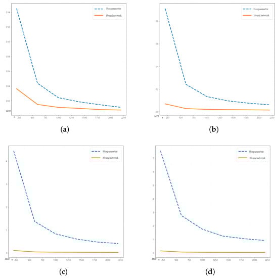
Figure 1.
of local linear regression method (dashed blue line) and the neural network method (solid orange line) of dimension 3, 5, 8 and 10. (a) Three dimensions. (b) Five dimensions. (c) Eight dimensions. (d) Ten dimensions.
Next, we consider high-dimensional spatial models with dependency structures to compare the of the two methods mentioned above.
Model 2:
where , , and follows a zero-mean second-order stationary process. follows a standard normal distribution. Similarly to the work of Cressie and Wikle [12], high-dimensional spatial processes are generated using spectral methods.
In this case, for follows a standard normal distribution and is independent of for , where are independently and identically distributed from a uniform distribution on . As , converges to a Gaussian random process. We consider the case with dimension 5 and sample sizes [200, 600, 1000, 1400, 1800, 2200]. The network structure is the same as in Model 1.
As shown in Table 2, it can be observed that the convergence rate of the high-dimensional spatial model with dependence is worse than the convergence rate of the high-dimensional spatial model without dependence. However, in comparison to the local linear regression method, the values of the neural network are much smaller, indicating that the neural network achieves better convergence performance.
Table 2.
The values of both methods for Model 2.
As shown in Figure 2, we see that in the case of large sample sizes and high-dimensional spatial models, the neural network achieves superior convergence compared to that of the local linear regression method, where the x-axis represents the sample size n, and the y-axis represents the mean squared error ().
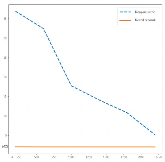
Figure 2.
Comparison of between two methods for Model 2.
3.2. Case Study
To compare the consistency of the local linear regression method and deep neural network for high-dimensional spatial models, we consider the relationship between air pollution and respiratory diseases in the New Territories East of Hong Kong from 1 January 2000 to 15 January 2001, as studied by Wang et al. [13]. There is a dataset consisting of 821 observations, where we mainly consider the air pollution index and five pollutants, sulfur dioxide () , inhalable particulate matter () , nitrogen compounds () , nitrogen dioxide () , and ozone () , as well as two environmental factors: temperature (C) and relative humidity (%) . In this section, we examine the relationship between the levels of chemical pollutants in the New Territories East of Hong Kong and the daily hospital admissions for respiratory diseases (Y). The specific parameter settings are the same as those in the numerical simulation part.
After dimensionless and standardization processing, we use 397 data points for the case study. Among these, 80% of the data are used to train the model, and the remaining 20% are used to evaluate the quality of the trained model. The values are shown in Table 3. It can be observed that the values are closer to 0, indicating that in real-world cases, the mean squared error of the deep neural network method is much smaller than that of the local linear regression method. Therefore, the deep neural network shows better convergence performance.
Table 3.
The values of both methods for this case.
Figure 3 presents a visual representation of the values for both methods, where the x-axis represents the sample size n, and the y-axis represents the mean squared error (). From the graph, it is evident that the deep neural network method exhibits a faster convergence rate compared to that of the local linear regression method.
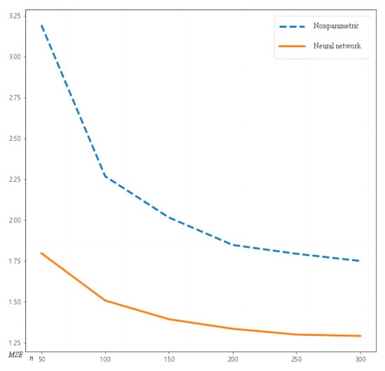
Figure 3.
Comparison of between two methods for this case.
4. Conclusions
In this study, we employ neural networks with ReLU activation functions for nonparametric estimation in high-dimensional spaces. By constructing suitable network architectures, we estimate unknown trend functions and prove the consistency of the estimators while also comparing and analyzing the deep neural network approach with traditional nonparametric methods.
The focus is on high-dimensional space models with unknown error distributions. Considering the spatial dependencies and heterogeneity in the space models, a deep neural network with ReLU activation functions is used to estimate the unknown trend functions. Under general assumptions, the consistency of the estimators is established, and bounds for the mean squared error () are provided. The estimators exhibit a convergence rate that is related to the sample size but independent of the dimensionality d, thereby avoiding the curse of dimensionality. Moreover, the proposed estimators achieve convergence speeds close to optimality.
Considering the spatial dependencies in high-dimensional settings with large sample sizes, the deep neural network method outperforms traditional nonparametric estimation methods.
Author Contributions
Methodology, H.W.; software & writing, X.J.; editing, H.H.; review J.W. All authors have read and agreed to the published version of the manuscript.
Funding
This research was funded by National Social Science Fund of China, grant number 22BTJ021.
Data Availability Statement
Not applicable.
Conflicts of Interest
The authors declare no conflict of interest.
Appendix A. The Embedding Property of Network Function Classes
To approximate functions by using neural networks, we first construct smaller networks to compute simpler objects. Let and . To merge networks, the following rules are commonly used in this paper.
Enlargement: , and .
Composition: Let and , where . For a vector , in the space , i.e., , the composition network is defined.
Additional Layer/Depth Synchronization: To synchronize the number of hidden layers in two networks, an additional layer can be added with a unit weight matrix, such that
Parallelization: Let f and g be two networks with the same number of hidden layers and the same input dimension, i.e., and , where . The parallel network computes both f and g simultaneously in the joint network class .
Removing Inactive Nodes: We have
In this context, we have . Let . If all entries in the j-th column of are zero, we can remove this column along with the j-th row of and the j-th element of without changing the function. This implies that . Since there are s active parameters, for any , we need to iterate at least times. This proves that .
In this paper, we often utilize the following fact. For a fully connected network in , there are weight matrix parameters and network parameters from bias vectors. Therefore, the total number of parameters is
Appendix B. Approximation by Polynomial Neural Networks
We construct a network with all parameters bounded by 1 to approximate the calculation of for given inputs x and y. Let , where k is a positive integer.
and , where
Next, we prove that converges exponentially to as m increases, especially in :. This lemma can be seen as a variation of Lemma 2.4 in Telgarsky’s work [14] and Proposition 2 in Yarotsky’s work [15]. Compared to existing results, this result allows us to construct networks with parameters equal to 1 and provides an explicit bound on the approximation error.
Lemma A1.
For any positive integer m,
Proof.
Step 1: We prove by induction that is a triangular wave. More precisely, is piecewise linear on the intervals , where ℓ is an integer. If ℓ is odd, the endpoints are , and if ℓ is even, the endpoints are .
When , the equality holds obviously.
We assume that the statement holds for k, and we let be divisible by 4, denoted as . Consider x in the interval . When , then . When , then . When , where , then . When , then . Then, for , the statement also holds.
The statement holds for , and the induction is complete.
Step 2: For convenience, let us denote . We now prove that for any and , the following holds:
To prove this, we use mathematical induction on m. For , when , we have and . When , we have and . When , we have and . holds. Therefore, for the inductive step, assuming that it holds for m, when is considered, if ℓ is even, then , which implies . If ℓ is odd, then the function is linear over the interval . Furthermore, for any t, we have
Since and , and considering ℓ such that , we can deduce
and the result also holds for , completing the induction.
Thus, the interpolation of at the point with function g has been proven, and it is linear over the interval . Let ; g is a Lipschitz function with Lipschitz constant 1. Therefore, for any x, there exists an ℓ determined by
and we have
which implies
thus proving the lemma.
Let . As proven above, to construct a network that takes inputs x and y and approximates the product , we use polar-type identities.
□
Lemma A2.
For any positive integer m, there exists a network such that for all , and
and .
Proof.
Let , where and . Consider a nonnegative function .
Step 1: We prove the existence of a network with m hidden layers and width vector to compute this function:
for all , as shown in Figure A1; it is worth noting that all parameters in this network are bounded by 1.
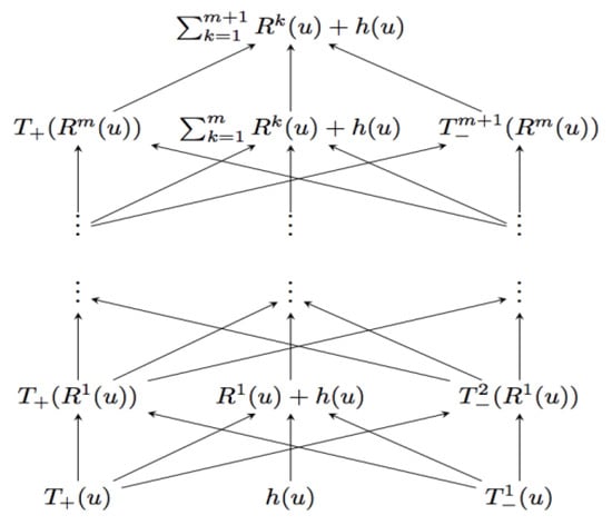
Figure A1.
Network .
Step 2: We prove the existence of a network with m hidden layers to compute the following functions:
Given the input , the computation of this network in the first layer is as follows:
Applying the network on the first three elements and the last three elements, we obtain a network with hidden layers and a width vector of , and we compute
applying the two-hidden-layer network to the output. Therefore, the composite network has hidden layers and computes
and this implies that the output is always in the interval . According to Equation (A4) and Lemma A1, we can obtain the following:
For all , we have and . Therefore, when k is odd, ; when k is even, . For all input pairs and , the output in Equation (A5) becomes zero. □
Lemma A3.
For any positive integer m, there exists a network
such that , for all , and we have
Furthermore, if one of the components of is 0, then .
Proof.
Let . We now construct the network and perform calculations in the first hidden layer.
We apply the network from Lemma A2 to each pair to compute , , and Mult Now, we pair adjacent terms and apply again. We continue this process until only one term remains. The resulting network is denoted as , which has hidden layers, and all parameters are bounded by 1.
If , then by Lemma A2 and the triangle inequality, we have
therefore, by iteration and induction, we obtain
By using Lemma A2 and the construction described above, it is evident that if one of the components of is 0, then
We construct a sufficiently large network to approximate all monomials for nonnegative integers up to a certain specified degree. Typically, we use multi-index notation: , where and represents the degree of the monomial.
The number of monomials with degrees satisfying is denoted by , and since each takes values in , we have . □
Lemma A4.
For and positive integers m, there exists a network
such that , and for all , we have
Proof.
For , the monomials are either linear or constant functions. There exists a shallow network in the class that precisely represents the monomial .
Considering the multiplicities in Equation (A6), Lemma A3 can be directly extended to monomials. For , this implies that in the class
there exists a network in the class that takes values within the interval and approximates to a supnorm error of . By utilizing the parallelization and depth synchronization properties discussed in Appendix B, the proof of Lemma A4 can be established.
Following the classical local Taylor approximation, previously used for network approximation by Yarotsky [15], for a vector , we define
According to Taylor’s theorem for multivariable functions, for an appropriate , we have
We have . Therefore, for , we have
We can express Equation (A7) as a linear combination of monomials.
for suitable coefficients , and, for convenience, the dependence on in is omitted here. Since , it follows that
and since and , we have
We consider the grid points . The number of elements in this set is . Let represent the elements of . We define
□
Lemma A5.
If , then .
Proof.
For all , we have
and we use mathematical induction, assuming . The left-hand side of (A11) is
and after summing, we obtain
while the middle-hand side, we have
and therefore the equation holds when .
Assuming , we have with ; Then, the left-hand side is
and after summation, we obtain
In the middle, we have
and, therefore, when , the equation holds true.
Next, we calculate the second equation in (A11); when , we have
and when ℓ takes values , the sum above is zero, resulting in 1. By analogy, for , where , the same holds true. Therefore, we can deduce that .
By using and Equation (A8), we obtain
Then, we describe how to construct a network that approximates . □
Lemma A6.
For any positive integers M and m, there exists a network
where , such that , and for any , we have
For any , the support of the function is contained within the support of the function .
Proof.
The first hidden layer uses units and nonzero parameters to compute the functions and . The second hidden layer uses units and nonzero parameters to compute the function . These functions take values in the interval , and the result holds when .
For , we combine the obtained network with the network approximating the product . According to Lemma A3, there exists a network Mult in the following class:
We compute with an error bounded by . From Equation (A3), it follows that a Mult network has nonzero parameters
as a bound, and since these networks have parallel instances, each hidden layer requires units and nonzero parameters for multiplication operations. Adding the nonzero parameters from the first two layers, the total bound on the number of nonzero parameters is
According to Lemma A3, if one of the components of is zero, then Mult . This implies that for any , the support of the function is contained within the support of the function . □
Theorem A1.
For any function and any integers and , there exists a network
with a depth of
and the number of parameters
such that
Proof.
In this proof, all constructed networks take the form , where . Let M be the largest integer such that , and we define . With the help of Equations (A9) and (A10), and Lemma A4, we can add a hidden layer to the network , resulting in a new network
such that and for any , we have
where and e is the natural logarithm. According to Equation (A3), the number of nonzero parameters in network is bounded by .
According to Lemma A6, the network calculates the product with an error bounded by . It requires at most active parameters. Now, consider the parallel network . Based on the definition of and the assumption on N, we observe that . According to Lemma A6, networks and can be embedded into a joint network with hidden layers. The weight vector and all parameters are bounded by 1. By using , the bound on the number of nonzero parameters in the combined network is
where, for the last inequality, we use , the definition of , and the property that for any , we have .
Next, we pair the outputs of and corresponding to the term and apply the Mult network described in Lemma A2 to each of the pairs. In the final layer, we sum all the terms together. According to Lemma A2, this requires at most active parameters for the total multiplications. By using Lemmas A2 and A6, Equation (A12), and the triangle inequality, we can construct a network
such that, for any , we have
where the first inequality follows from the fact that the support of is contained within the support of , as stated in Lemma A6. Due to Equation (A3), the network has at most
To obtain the network reconstruction of the function f, it is necessary to apply scaling and shifting to the output terms. This is primarily due to the finite parameter weights in the network. We recall that . The network belongs to the class , where the shift vectors are all zero and all entries of the weight matrices are equal to 1. Since , the number of parameters in this network is bounded by . This implies the existence of a network in the class , which computes , where . This network computes and in the first hidden layer, and then applies the network to these two units. In the output layer, the first value is subtracted from the second value. This requires at most active parameters.
Due to Equations (A11) and (A14), there exists a network in the following class
and for all , we have
Under the condition of Equation (A15), the bound for the nonzero parameters of is
By constructing , it follows that . Combined with Lemma A5, we have
Thus, the result is proven.
Based on Theorem A1, we can now construct a network that approximates . In the first step, we show that f can always be represented as a composition of functions defined on hypercubes . As in the previous theorem, let , and we assume for . Define
where means applying the transformation to all j. It is evident that
From the definition of the Hölder ball , we can see that takes values in the interval .
where, for , we have . Without loss of generality, we can always assume that the radius of the Hölder ball is at least 1, i.e., . □
Lemma A7.
Let be as defined above, with . Then, for any function , where , we have
Proof.
Let and . If is an upper bound of the Hölder seminorm of for , then, by the triangle inequality, we have
Combining this with the inequality , which holds for all and all , the lemma is proven. □
Proof of Theorem 1.
Here, all n are assumed to be sufficiently large. Throughout the entire proof, is a constant that depends only on the variation of . Combining Theorem 2 with the bounds on the depth L and network sparsity s assumed, for , we have
where, for the lower bound, we set , and for the upper bound, we set . We take ; then, when , we have . Substituting this into the left-hand side of Equation (A17), we obtain
that is,
Thus, the lower bound for Equation (8) is established.
To obtain upper bounds for Equations (7) and (8), it is necessary to constrain the approximation error. For this purpose, the regression function m is rewritten as Equation (A16), i.e., , where and is defined on and maps to for any .
Here, we apply Theorem A1 to each function separately. Let and consider the following.
this means that there exists a network
where , such that
where is the Hölder norm upper bound of . If , two additional layers are applied to the output, requiring four additional parameters. The resulting network is denoted as
and it is observed that . Since , we have
If the network is parallelized, belongs to the class
where . Finally, constructing the composite network , according to the construction rules in Appendix A, we can realize it in the following class:
where . By observation, there exists an bounded by n such that
For all sufficiently large n, utilizing the inequality , we have , according to Equation (A1), and for sufficiently large n, the space defined in Equation (A20) can be embedded into , where satisfies the assumptions of the theorem. We choose with a sufficiently small constant , depending only on . Combining Theorem A1 with Equations (A18) and (A19), we have
For the approximation error in Equation (A17), we need to find a network function bounded by the supnorm of F. According to the previous inequalities, there exists a sequence of functions such that, for all sufficiently large n, , and . Let us define . Then, , where the last inequality is based on Assumption (1). Additionally, . We can denote , and we have , which implies . This shows that if we take the lower bound on a smaller space , then Equation (A21) also holds. Combining this with the upper bound of Equation (A17), we obtain when , that
and when , that
therefore, the upper bounds in Equations (7) and (8) hold for any constant . This completes the proof.
We begin by utilizing several oracle inequalities for the least squares estimators, as presented in Gyo et al. [16,17,18,19,20]. However, these inequalities assume bounded response variables, which are violated in the nonparametric regression model with Gaussian measurement noise. Additionally, we provide a lower bound for the risk and offer proof that can be easily generalized to any noise distribution. Let be the covering number, which represents the minimum number of balls with radius needed to cover (where the center does not necessarily have to be within ). □
Lemma A8.
We consider the nonparametric regression model in d-dimensional variables given by Equation (2) with an unknown regression function m. Let be an arbitrary estimator taking values in . Let us define
For and assuming . If , for any , then
Proof.
Throughout the proof, let . Define . For any estimator , we introduce the empirical risk .
Step 1: We show that the upper bound holds under the restriction . Since , the upper bound naturally holds when . In this case, let be a global risk minimizer. We observe that
From this equation, we see that , which implies a lower bound on the logarithm in the argument.
Therefore, we assume that . The proof is divided into four parts, denoted as (I)–(IV).
- (I)
- Establishing a connection between risk and its empirical counterpart through inequalities
- (II)
- For any estimate taking values in , we know that
- (III)
- We have
- (IV)
- We have
Since , the lower bound of the lemma can be obtained by combining (I) and (IV), while the upper bound can be obtained from (I) and (III).
(I) Given a minimum -covering of , let represent the centers of the balls. According to the construction, there exists a random such that . Without loss of generality, we can assume that . The random variables , have the same distribution as and are independent of . We can use
where . We replace with , and we define by using the same method. Similarly, we set , and define as when .
In the last part, we use the triangle inequality and
For random variables U and T, the Cauchy–Schwarz inequality states that . Let
and
By using , we have
Observing that ,
and
Bernstein’s inequality states that for independent and centered random variables , if then it holds true that [21]
Combining Bernstein’s inequality and the bound argument, we obtain
and since , for all , we have
Thus, for large values of t, the denominator in the exponential is dominated by the first term. We have
According to the assumption, ; hence, . By using a similar approach to the upper bound for , we can obtain the quadratic case.
Step 2: The identity . In this case, we set and to obtain the aforementioned inequality.
Let be positive real numbers such that . We have
Consequently, for any , we have the following.
According to Equation (A24), we take , , and . Substituting into Equation (A25) (denoted as (I)), we complete the proof of (I).
(II) Given an estimation that takes values in , let be such that . Then, . Since , we have
where
Under the condition , . According to Lemma A9, we obtain . By using Cauchy–Schwarz, we have
Since , we have . Combining Equations (A26) and (A27), we have
(II) is proven.
(III) For any fixed , we have . Since and f are deterministic, we have
. Since , we have
By setting in Equation (A25), we obtain the result for (III).
(IV) Let be the empirical risk minimizer. By using Equation (A22), (II), and , we have
After rearranging, we have , which completes the proof of (IV). □
Lemma A9.
Let , and then .
Proof.
Let . Since , and we have . For , it is evident that holds. Therefore, we consider the case when . By using Mill’s ratio, we obtain . For any T, we have
For and , we have
Since , we can deduce that . Considering that the function is monotonically increasing with respect to M, it holds for all . □
Lemma A10.
If , then for any , we have
Proof.
Given a network
define ,
and ,
Let , and we note that for , we have . For a multivariate function , is said to be a Lipschitz function if, for all in its domain, , where the smallest L is the Lipschitz constant. The combination of two Lipschitz functions with Lipschitz constants and results in a new Lipschitz function with a Lipschitz constant of . Therefore, the Lipschitz constant of is bounded by . Given , let be two network functions with parameters differing from each other by at most . Let f have parameters and have parameters . Then, we have
The final step uses . Therefore, according to Equation (A3), the total number of parameters is bounded by , and there are combinations to select s nonzero parameters.
Since all parameters are bounded by 1 in absolute value, we can discretize the nonzero parameters by using a grid size of , and the covering number
Taking the logarithm yields the proof.
Note 1: Similarly, applying Equation (A4) to Lemma A10 gives
□
Proof of Theorem 2.
Let . The proof follows directly from Lemmas A8 and A10, and Note 1. □
Proof of Theorem 3.
In this proof, we define . Let us assume that there exist positive constants such that the Lebesgue density of over is bounded below by and above by . For this particular design, we have . Let represent the data mechanism in the nonparametric regression model given by Equation (13). For the Kullback–Leibler divergence, we have . In Alexandre’s work [22], Theorem 2.7 states that if, for and , we have , then
(i) , where ;
(ii) .
Then, there exists a positive constant such that
In the next step, we construct functions satisfying (i) and (ii). We define
The exponent determines the rate of estimation, i.e., . For convenience, we denote , and . We note the distinction between and . Let be supported on . It is easy to see that such a function K exists. Furthermore, we define and , where is a constant chosen so that , with . For any , we define
and for any and , we have , by using the fact that .
For with , the triangle inequality and the property give
therefore, . For a vector , we define
By constructing and for such that are mutually disjoint, we ensure that (.
For , let . For , define . For , let . Here, . We frequently use . Since and the mutually disjoint ensures
by choosing a sufficiently large K, we ensure that .
For all , . Let denote the Hamming distance; then,
According to the Varshamov–Gilbert bound (see [22], Lemma 2.9) and , there exists a subset with a cardinality of . For all such that , it holds that . This implies that for all , we have
According to the definitions of and , we have
This indicates that the functions with satisfy (i) and (ii), and, thus, the lemma is proven. □
Proof of Lemma 1.
Let . Since , we need to consider only the lower bound on , where . Let be the empirical risk minimizer. Recall that . Due to the minimax lower bound in Theorem 3, there exists a constant such that for all sufficiently large n, we have . Since and , by Theorem 2, we can conclude that
where C is a constant. Given , let . If , and , and , then, for sufficiently small and all , we can insert into the previous inequalities, and we have
The constants and depend only on and d. By using the condition and choosing a sufficiently small , the proof is completed. □
Proof of Lemma 2.
Let r be the smallest positive integer such that . Such an r exists because the span of is dense in , and cannot be a constant function. If , then, for the wavelet coefficients, we have
For a real number u, let denote the fractional part of u.
We separately consider the cases when and . If , we define . We note that g is a Lipschitz function with Lipschitz constant 1. Let , where , . For a V-periodic function , —Hölder can be expressed as
Since g is a 1-Lipschitz function, for any u and v such that , we have
Therefore, and . Let . The support of is contained in and . Based on the definition of wavelet coefficients, Equation (A28), the definition of , and using , for , we have
In the last equation, according to the definition of r, .
In the case of , we take . Following the same reasoning as above and by using the binomial theorem, we obtain
therefore, the lemma is proven. □
Proof of Theorem 4.
We define as in Lemma 2. We choose an integer such that
This implies that . According to Lemma 2, there exists a function of the form , where , such that
therefore, the lemma is proven. □
References
- Hallin, M.; Lu, Z.; Tran, L.T. Local linear spatial regression. Ann. Stat. 2004, 32, 2469–2500. [Google Scholar] [CrossRef]
- Biau, G.; Cadre, B. Nonparametric spatial prediction. Stat. Inference Stoch. Process. 2004, 7, 327–349. [Google Scholar] [CrossRef]
- Bentsen, L.; Warakagoda, N.D.; Stenbro, R.; Engelstad, P. Spatio-temporal wind speed forecasting using graph networks and novel Transformer architectures. Appl. Energy 2023, 333, 120565. [Google Scholar] [CrossRef]
- Du, P.; Bai, X.; Tan, K.; Xue, Z.; Samat, A.; Xia, J.; Li, E.; Su, H.; Liu, W. Advances of four machine learning methods for spatial data handling: A review. J. Geovis. Spat. Anal. 2020, 4, 13. [Google Scholar] [CrossRef]
- Farrell, A.; Wang, G.; Rush, S.A.; Martin, J.A.; Belant, J.L.; Butler, A.B.; Godwin, D. Machine learning of large-scale spatial distributions of wild turkeys with high-dimensional environmental data. Ecol. Evol. 2019, 9, 5938–5949. [Google Scholar] [CrossRef] [PubMed]
- Nikparvar, B.; Thill, J.C. Machine learning of spatial data. ISPRS Int. J. -Geo-Inf. 2021, 10, 600. [Google Scholar] [CrossRef]
- Schmidt-Hieber, J. Nonparametric regression using deep neural networks with ReLU activation function. Ann. Stat. 2020, 48, 1875–1897. [Google Scholar]
- Wang, H.; Wu, Y.; Chan, E. Efficient estimation of nonparametric spatial models with general correlation structures. Aust. N. Z. J. Stat. 2017, 59, 215–233. [Google Scholar] [CrossRef]
- He, K.; Zhang, X.; Ren, S.; Sun, J. Deep residual learning for image recognition. In Proceedings of the IEEE Conference on Computer Vision and Pattern Recognition, Las Vegas, NV, USA, 27–30 June 2016; pp. 770–778. [Google Scholar]
- He, K.; Sun, J. Convolutional neural networks at constrained time cost. In Proceedings of the IEEE Conference on Computer Vision and Pattern Recognition, Boston, MA, USA, 7–12 June 2015; pp. 5353–5360. [Google Scholar]
- Cohen, A.; Daubechies, I.; Vial, P. Wavelets on the interval and fast wavelet transforms. Appl. Comput. Harmon. Anal. 1993, 1, 54–81. [Google Scholar] [CrossRef]
- Cressie, N.; Wikle, C.K. Statistics for Spatio-Temporal Data; John Wiley & Sons: Hoboken, NJ, USA, 2015. [Google Scholar]
- Wang, H.X.; Lin, J.G.; Huang, X.F. Local modal regression for the spatio-temporal model. Sci. Sin. Math. 2021, 51, 615–630. (In Chinese) [Google Scholar]
- Telgarsky, M. Benefits of depth in neural networks. In Proceedings of the Conference on Learning Theory, PMLR, Hamilton, New Zealand, 16–18 November 2016; pp. 1517–1539. [Google Scholar]
- Yarotsky, D. Error bounds for approximations with deep ReLU networks. Neural Netw. 2017, 94, 103–114. [Google Scholar] [CrossRef] [PubMed]
- Györfi, L.; Kohler, M.; Krzyzak, A.; Walk, H. A Distribution-Free Theory of Nonparametric Regression; Springer: New York, NY, USA, 2002. [Google Scholar]
- Giné, E.; Koltchinskii, V.; Wellner, J.A. Ratio limit theorems for empirical processes. In Stochastic Inequalities and Applications; Birkhäuser: Basel, Switzerland, 2003; pp. 249–278. [Google Scholar]
- Hamers, M.; Kohler, M. Nonasymptotic bounds on the L2 error of neural network regression estimates. Ann. Inst. Stat. Math. 2006, 58, 131–151. [Google Scholar] [CrossRef]
- Koltchinskii, V. Local Rademacher complexities and oracle inequalities in risk minimization. Ann. Stat. 2006, 34, 2593–2656. [Google Scholar] [CrossRef]
- Massart, P. Concentration Inequalities and Model Selection: Ecole d’Eté de Probabilités de Saint-Flour XXXIII-2003; Springer: Berlin/Heidelberg, Germany, 2007. [Google Scholar]
- Wellner, J. Weak Convergence and Empirical Processes: With Applications to Statistics; Springer Science and Business Media: Berlin/Heidelberg, Germany, 2013. [Google Scholar]
- Tsybakov, A.B. Introduction to Nonparametric Estimation; Springer Series in Statistics; Springer: New York, NY, USA, 2009. [Google Scholar]
Disclaimer/Publisher’s Note: The statements, opinions and data contained in all publications are solely those of the individual author(s) and contributor(s) and not of MDPI and/or the editor(s). MDPI and/or the editor(s) disclaim responsibility for any injury to people or property resulting from any ideas, methods, instructions or products referred to in the content. |
© 2023 by the authors. Licensee MDPI, Basel, Switzerland. This article is an open access article distributed under the terms and conditions of the Creative Commons Attribution (CC BY) license (https://creativecommons.org/licenses/by/4.0/).