The Fuzzy Differential Transform Method for the Solution of the System of Fuzzy Integro-Differential Equations Arising in Biological Model

Abstract

This article deals with the implementation of fuzzy differential transform method for solving a system of nonlinear fuzzy integro-differential equations. This system appears in a model of biological species living together. Though the differential transform method is an iterative method, the current approach reduces this model to a set of nonlinear algebraic equations due to its delay terms. The basic definitions and theorems are first presented. The applicability and accuracy of the current methodologies have been demonstrated through the discussion of a few exemplary situations.

1. Introduction

One of the key tools for many fields of applied mathematics is the integral equation. Many branches of science and engineering naturally contain integral equations [1]. Functional equations, such as partial differential equations, integral and integro-differential equations, stochastic equations, and others are frequently produced when real-world issues are mathematically modeled. Integro-differential equations are the common component of mathematical descriptions of physical events; they may be found in fluid dynamics, biological models, and chemical kinetics. Integro-differential equations arise in many numerous physical processes, including the formation of glass-forming process [2], nano-hydrodynamics [3], drop wise condensation [4], wind ripple in the desert [5] and biological model [6].

Many researchers are now focusing their research on the investigation of fuzzy integral equations and fuzzy differential equations. Zadeh [7,8] was the first to present the idea of fuzzy sets. By Kaleva and Seikkala [9,10], fuzzy integral equations were first developed. Many scholars have recently concentrated their attention on this area and written numerous studies that are available in the literature [11]. Fuzzy integral equations have been solved using a variety of analytical techniques, including the Adomian decomposition approach [12,13], homotopy analysis method [14], homotopy perturbation method [15], Laplace transform method [16] and Sumudu decomposition method [17]. Numerous numerical methods are available to solve fuzzy integral problems (see [18,19,20]).

In this work, we consider the following system of integro-differential equations as [6]

$$\begin{array}{c}\hfill \left\{\begin{array}{c}{p}^{{}^{\prime }}\left(z\right)=p\left(z\right)\left[a_1-{\lambda }_{1}q\left(z\right)-{\int }_{z-Z_0}^z{h}_1(z-\tau )q\left(\tau \right)d\tau \right]+l_1\left(z\right),0\le z\le T,a_1,{\lambda }_1>0,\\ q^{{}^{\prime }}\left(z\right)=q\left(z\right)\left[-a_2+{\lambda }_{2}p\left(z\right)+{\int }_{z-Z_0}^z{h}_2(z-\tau )p\left(\tau \right)d\tau \right]+l_2\left(z\right),0\le z\le T,a_2,{\lambda }_2>0,\end{array}\right.\end{array}$$

(1)

with initial conditions

$$p\left(0\right)={\alpha }_1,q\left(0\right)={\alpha }_2,$$

where $l_1\left(z\right),l_2\left(z\right),h_1\left(z\right),h_2\left(z\right)$ are given functions, $p\left(z\right),q\left(z\right)$ are unknown functions and $Z_0\in R$.

Here, the numbers of two distinct species at time z are $p\left(z\right)$ and $q\left(z\right)$, where the first species grows and the second shrinks. In the event that they exist together, assuming that the second species would consume the first, there will be a rise in the second species’ rate, or $\frac{dq}{dz}$, which depends on both the first species’ historical values and its current populations, or $p\left(z\right)$. The coefficients of increase and decrease for the first and second species, respectively, are $a_1$ and $-a_2$. The values of the parameters ${\lambda }_1,{\lambda }_2$ and the kernels $h_1\left(z\right)$, $h_2\left(z\right)$ are dependent on the species.

In our work, we have considered this model in fuzzy sense, i.e., if $p\left(z\right),q\left(z\right),l_1\left(z\right)$ and $l_2\left(z\right)$ are fuzzy functions, these functions can be expressed in parametric form as $(\underline{p}(z,\beta ),\overline{p}(z,\beta ))$, $(\underline{q}(z,\beta ),\overline{q}(z,\beta ))$, $(\underline{l_1}(z,\beta ),\overline{l_1}(z,\beta ))$ and $(\underline{l_2}(z,\beta ),\overline{l_2}(z,\beta ))$, respectively.

The classical higher order Taylor series approach, which needs symbolic computation of the required derivatives of the data function and is computationally costly for higher order, is different from the differential transform method. The approximate solution is assessed using the finite Taylor series via the differential transformation technique. However, the differential transform technique does not compute the derivative directly; rather, the relative derivatives are generated through an iterative process. Allahviranloo et al. [21] have suggested fuzzy differential transform method (FDTM) in order to solve first order fuzzy differential equations under generalized differentiability. The fuzzy integro-differential equations, higher order fuzzy differential equations, fuzzy boundary value problems, etc. may all be simply added to the scope of this technique. In this article, the above said biological model has been solved by fuzzy differential transform method. The FDTM has been applied by many authors to solve integral equations and integro-differential equations [22,23,24].

This paper has been organized as follows: in Section 2, some fundamental terminologies and outcomes that will be utilized later are brought. For the purpose of solving a fuzzy system of integral equations, a fuzzy differential transform method is presented in Section 3. In Section 4, we study the main result. The proposed approach is used to resolve three illustrative cases in Section 5. Section 6 draws conclusions.

2. Preliminaries

The most fundamental fuzzy calculus notations are introduced in this section. To begin, a fuzzy number is defined.

Definition 1 ([19]). 

An ordered pair of functions $\left(\underline{v}\left(\beta \right),\overline{v}\left(\beta \right)\right)$; $0\le \beta \le 1$ that match the following conditions can be used to describe a fuzzy number v.

1. 

$\underline{v}\left(\beta \right)$ is a left continuous monotonic bounded increasing function.

2. 

$\overline{v}\left(\beta \right)$ is a is a left continuous monotonic bounded decreasing function.

3. 

$\underline{v}\left(\beta \right)\le \overline{v}\left(\beta \right),0\le \beta \le 1$.

For arbitrary $v=\left(\underline{v},\overline{v}\right)$, $w=\left(\underline{w},\overline{w}\right)$ and $k>0$, we define addition $(v+w)$ and scalar multiplication by k as

a. 

$\left(\underline{v+w}\right)\left(\beta \right)=\underline{v}\left(\beta \right)+\underline{w}\left(\beta \right)$

b. 

$\left(\overline{v+w}\right)\left(\beta \right)=\overline{v}\left(\beta \right)+\overline{w}\left(\beta \right)$

c. 

$\left(\underline{kw}\right)\left(\beta \right)=k\underline{w}\left(\beta \right)$, $\left(\overline{kw}\right)\left(\beta \right)=k\overline{w}\left(\beta \right)$

Since each $y\in \mathbb{R}$ can be regarded as a fuzzy number $\tilde{y}$ defined by

$$\tilde{y}\left(t\right)=\left\{\begin{array}{cc}1\hfill & \mathrm{if}t=y\hfill \\ 0\hfill & \mathrm{if}t\ne y\hfill \end{array}\right.$$

Let $\mathbb{E}$ be the set of all upper semicontinuous normal convex fuzzy numbers with bounded $\beta$-level intervals, the Hausdorff distance between fuzzy numbers given by $D:\mathbb{E}\times \mathbb{E}\to {\mathbb{R}}_{+}\cup \left\{0\right\}$ such that

$$D(u,w)=\underset{0\le \beta \le 1}{sup}\left[\max \left\{|\overline{u}\left(\beta \right)-\overline{w}\left(\beta \right)|,|\underline{u}\left(\beta \right)-\underline{w}\left(\beta \right)|\right\}\right].$$

It is easy to see that D is a metric in $\mathbb{E}$ and has the following properties [11].

a.

$D(u\oplus v,w\oplus v)=D(u,w)$; $\forall u,w\in \mathbb{E}.$

b.

$D(k\odot u,k\odot w)=\left|k\right|D(u,w);\forall k\in \mathbb{R},\forall u,w\in \mathbb{E}.$

c.

$D(u\oplus v,w\oplus e)\le D(u,w)+D(v,e);\forall u,w,v,e\in \mathbb{E}.$

d.

$(\mathbb{E},D)$ is a complete metric space.

Definition 2. 

Let $f:\mathbb{R}\to \mathbb{E}$ be a fuzzy valued function. If for arbitrary fixed $t_0\in \mathbb{R}$ and $\epsilon >0$, there exists a $\delta >0$ such that $\left|t-t_0\right|<\delta \Rightarrow D(f\left(t\right),f\left(t_0\right))<\epsilon ; f$ is said to be continuous. It is well-known that the H-derivative (differentiability in the sense of Hukuhara) for fuzzy mappings was initially introduced by Puri and Ralescu [25] which is based on the H-difference of sets, as follows:

Definition 3. 

Let $x,y\in \mathbb{E}$. If there exists $z\in \mathbb{E}$ such that $x=y+z$, then z is called the H-difference of x and y, and it is denoted by $x⊝y$.

In this paper we consider the following definition which was introduced by Chalco–Cano and Román-Flores [26].

Definition 4. 

Let $f:(a,b)\to \mathbb{E}$ and $x_0\in (a,b)$. We say that f is differential at $x_0$, If there exists an element $f^{{}^{\prime }}\left(x_0\right)\in \mathbb{E}$, such that for all $h\ne 0$; $\exists f(x_0+h)⊝f\left(x_0\right)$ and $\exists f\left(x_0\right)⊝f(x_0-h)$ the limits (in the metric D) ${lim}_{h\to 0}\frac{f(x_0+h)⊝f\left(x_0\right)}{h}={lim}_{h\to 0}\frac{f\left(x_0\right)⊝f(x_0-h)}{h}=f^{{}^{\prime }}\left(x_0\right)$.

In this paper, we consider the nonlinear system of fuzzy integro-differential equation given in Equation (1), where $p(z;\beta ),q(z;\beta ),l_1(z;\beta ),l_2(z;\beta )$ are fuzzy valued functions, and the signs of $h_1\left(z\right)$ and $h_2\left(z\right)$ do not change in $[0,1]$. Let

$$p(z;\beta )=(\underline{p}(z;\beta ),\overline{p}(z;\beta ))$$

$$q(z;\beta )=(\underline{q}(z;\beta ),\overline{q}(z;\beta ))$$

$$l_1(z;\beta )=(\underline{l_1}(z;\beta ),{\overline{l}}_1(z;\beta ))$$

$$l_2(z;\beta )=({\underline{l}}_2(z;\beta ),{\overline{l}}_2(z;\beta ))$$

Equation (1) can be transformed into two systems as

$$\begin{array}{c}\hfill \left\{\begin{array}{c}\underline{p^{{}^{\prime }}}(z;\beta )=\underline{p}(z;\beta )\left[a_1-{\lambda }_1\underline{q}(z;\beta )-{\int }_{z-Z_0}^z{h}_1(z-\tau )\underline{q}(\tau ;\beta )d\tau \right]+\underline{l_1}(z;\beta ),0\le z\le T,a_1,{\lambda }_1>0,\\ \underline{q^{{}^{\prime }}}(z;\beta )=\underline{q}(z;\beta )\left[-a_2+{\lambda }_2\underline{p}(z;\beta )+{\int }_{z-Z_0}^z{h}_2(z-\tau )\underline{p}(\tau ;\beta )d\tau \right]+\underline{l_2}(z;\beta ),0\le z\le T,a_2,{\lambda }_2>0\end{array}\right.\end{array}$$

(2)

$$\begin{array}{c}\hfill \left\{\begin{array}{c}\overline{p^{{}^{\prime }}}(z;\beta )=\overline{p}(z;\beta )\left[a_1-{\lambda }_1\overline{q}(z;\beta )-{\int }_{z-Z_0}^z{h}_1(z-\tau )\overline{q}(\tau ;\beta )d\tau \right]+\overline{l_1}(z;\beta ),0\le z\le T,a_1,{\lambda }_1>0,\\ \overline{q^{{}^{\prime }}}(z;\beta )=\overline{q}(z;\beta )\left[-a_2+{\lambda }_2\overline{p}(z;\beta )+{\int }_{z-Z_0}^z{h}_2(z-\tau )\overline{p}(\tau ;\beta )d\tau \right]+\overline{l_2}(z;\beta ),0\le z\le T,a_2,{\lambda }_2>0\end{array}\right.\end{array}$$

(3)

3. Fuzzy Differential Transform Method

Let us consider $p\left(z\right)=(\underline{p}(z;\beta ),\overline{p}(z;\beta ))$ is differentiable of order k over time z, then

$${\underline{P}}_i(k;\beta )=\frac{d^k\underline{p}(z;\beta )}{d{z}^k}{\mid }_{z=z_i},{\overline{P}}_i(k;\beta )=\frac{d^k\overline{p}(z;\beta )}{d{z}^k}{\mid }_{z=z_i},\forall k\in K=0,1,2,\cdots$$

$\underline{P_i}(z;\beta )$ and $\overline{P_i}(z;\beta )$ are called lower and upper spectrum of $p\left(z\right)$ at $z=z_i$, respectively. So if $p\left(z\right)$ be differentiable, then $p\left(z\right)$ can be represented as

$$\underline{p}(z;\beta )=\sum _{k=0}^{\infty }\frac{{(z-z_i)}^k}{k!}\underline{P}(k;\beta ),0\le \beta \le 1,$$

$$\overline{p}(z;\beta )=\sum _{k=0}^{\infty }\frac{{(z-z_i)}^k}{k!}\overline{P}(k;\beta ),0\le \beta \le 1.$$

The mentioned equations are known as the inverse transformation of $\underline{P}(k;\beta )$ and $\overline{P}(k;\beta )$, respectively. The more conceptual definitions and theorems related to fuzzy differential transform are available in [11].

Theorem 1 ([11]). 

Let’s assume that $s(z;\beta )$ and $t(z;\beta )$ are fuzzy-valued functions and $S(u;\beta )$ and $T(u;\beta )$, respectively, represent their fuzzy differential transformations. Then

$\left(a\right)$

If $m(z;\beta )=s(z;\beta )+t(z;\beta )$, then $M(u;\beta )=S(u;\beta )+T(u;\beta ),u\in U$,

$\left(b\right)$

If $m(z;\beta )=s(z;\beta )-t(z;\beta )$, then $M(u;\beta )=U(u;\beta )-T(u;\beta ),u\in U$.

$\left(c\right)$

If $m(z;\beta )=s(z;\beta )\ominus t(z;\beta )$, then $M(u;\beta )=U(u;\beta )\ominus T(u;\beta ),u\in U$.

Provided the Hukuhara difference exists.

Theorem 2 ([11]). 

Consider the fuzzy-valued functions $l\in \mathbb{E}$ and $h(x;\beta )={\int }_{x_0}^{x}l(t;\beta )dt$, then $H(u;\beta )=\frac{G(u-1;\beta )}{u}$, where $H(u;\beta )$ and $G(u;\beta )$ are the differential transformations of h and l, respectively.

Theorem 3 ([11]). 

Let us consider $h(x;\beta )={\int }_{x_0}^x{\int }_{x_0}^{x_{n-1}}\cdots {\int }_{x_0}^{x_1}l(t;\beta )dtd{x}_{1}d{x}_2\cdots d{x}_{n-1}$, then $H(u;\beta )=\frac{(u-n)!}{u!}G(u-n;\beta )$ where $H(u;\beta )$ and $G(u;\beta )$ are the fuzzy differential transformations of fuzzy-valued functions h and l, respectively.

Theorem 4 ([11]). 

Assume that $S(u;\beta )$ and $T(u;\beta )$ are fuzzy differential transformations of $s(z;\beta )$ and $t(z;\beta )$ respectively. Under (i)—differentiability of f, if $f(z;\beta )={\int }_{z_0}^{z}t(x;\beta )s(x;\beta )dx$ then

$\left(a\right)$

$\underline{F}(u;\beta )={\sum }_{n=0}^{u-1}T\left(n\right)·\frac{\underline{S}(u-n-1;\beta )}{n};0\le \beta \le 1$.

$\left(b\right)$

$\overline{F}(u;\beta )={\sum }_{n=0}^{u-1}T\left(n\right)·\frac{\overline{S}(u-n-1;\beta )}{n};0\le \beta \le 1.$

And under (ii)—differentiability of f we have

$\left(c\right)$

$\underline{F}(u;\beta )={\sum }_{n=0,even}^{u-1}T\left(n\right)·\frac{\underline{S}(u-n-1;\beta )}{n}+{\sum }_{n=1,odd}^{u-1}T\left(n\right)·\frac{\underline{S}(u-n-1;r)}{n}F(0;\beta )=\tilde{0};0\le \beta \le 1.$

$\left(d\right)$

$\overline{F}(u;\beta )={\sum }_{n=0,even}^{u-1}T\left(n\right)·\frac{\overline{S}(u-n-1;\beta )}{n}+{\sum }_{n=1,odd}^{u-1}T\left(n\right)·\frac{\overline{S}(u-n-1;\beta )}{n}F(0;\beta )=\tilde{0};0\le \beta \le 1$.

Theorem 5 ([11]). 

Suppose that $S(u;\beta )$ and $T(u;\beta )$ are the fuzzy differential transformations of the functions $s(z;\beta )$ and $t(z;\beta )$ (is a positive real valued function), respectively. If $f(x;\beta )=s(z;\beta )t(z;\beta )$, then $F(n;\beta )={\sum }_{l=0}^{u}S(l;\beta )T(u-1;\beta )$

4. Main Results

We demonstrate a few theorems in this section that allow the FDTM to be extended to the systems (1) and (2).

Theorem 6. 

If $S(u;\beta )$ is the fuzzy differential transform of $s(z;\beta )$ at $z_0=\gamma$, then the fuzzy differential transform of $s(z;\beta )$ at $z_0=0$ is defined as $\overline{S}(u;\beta )={\sum }_{v=u}^{\infty }\overline{S}(v;\beta )\left(\genfrac{}{}{0pt}{}{v}{u}\right){(-\gamma )}^{v-u}$ and $\underline{S}(u;\beta )={\sum }_{u=v}^{\infty }\underline{S}(u;\beta )\left(\genfrac{}{}{0pt}{}{v}{u}\right){(-\gamma )}^{v-u}$.

Proof. 

Since

$$\begin{array}{cc}\hfill \underline{s}(z;\beta )& =\sum _{u=0}^{\infty }\underline{S}(u;\beta ){(z-\gamma )}^u\hfill \\ \hfill & =\sum _{u=0}^{\infty }\underline{S}(u;\beta )\left[\sum _{v=0}^u\left(\genfrac{}{}{0pt}{}{u}{v}\right)z^v{(-\gamma )}^{u-v}\right]\hfill \\ \hfill & =\sum _{u=0}^{\infty }\left[\sum _{v=u}^{\infty }\underline{S}(v;\beta )\left(\genfrac{}{}{0pt}{}{u}{v}\right){(-\gamma )}^{v-u}\right]z^v\hfill \end{array}$$

From the above, we get $\underline{S}(u;\beta )={\sum }_{v=u}^{\infty }\underline{S}(v;\beta )\left(\genfrac{}{}{0pt}{}{u}{v}\right){(-\gamma )}^{v-u}$ and

$$\begin{array}{cc}\hfill \overline{s}(z;\beta )& =\sum _{u=0}^{\infty }\overline{S}(u;\beta ){(z-\gamma )}^u\hfill \\ \hfill & =\sum _{u=0}^{\infty }\overline{S}(u;\beta )\left[\sum _{v=0}^u\left(\genfrac{}{}{0pt}{}{u}{v}\right)z^v{(-\gamma )}^{u-v}\right]\hfill \\ \hfill & =\sum _{u=0}^{\infty }\left[\sum _{v=u}^{\infty }\overline{S}(v;\beta )\left(\genfrac{}{}{0pt}{}{u}{v}\right){(-\gamma )}^{v-u}\right]z^v\hfill \end{array}$$

From the above, we get $\overline{S}(u;\beta )={\sum }_{v=u}^{\infty }\overline{S}(v;\beta )\left(\genfrac{}{}{0pt}{}{u}{v}\right){(-\gamma )}^{v-u}$. □

Theorem 7. 

If $S(u;\beta )$ is the fuzzy differential transform $s(z;\beta )$ at $z_0=0$, then the fuzzy differential transform of $s(z;\beta )$ at $z_0=\gamma$ is $\overline{S}(u;\beta )={\sum }_{v=u}^{\infty }\overline{S}(v;\beta )\left(\genfrac{}{}{0pt}{}{v}{u}\right){\left(\gamma \right)}^{v-u}$ and $\underline{S}(u;\beta )={\sum }_{v=u}^{\infty }\underline{S}(v;\beta )\left(\genfrac{}{}{0pt}{}{v}{u}\right){\left(\gamma \right)}^{v-u}$.

Proof. 

We have

$$\begin{array}{cc}\hfill \underline{s}(z;\beta )& =\sum _{v=0}^{\infty }\underline{S}(v;\beta )z^v\hfill \\ \hfill & =\sum _{v=0}^{\infty }\underline{S}(v;\beta ){[(z-\gamma )+\gamma ]}^v\hfill \\ \hfill & =\sum _{v=0}^{\infty }\underline{S}(v;\beta )\sum _{u=0}^v\left(\genfrac{}{}{0pt}{}{v}{u}\right){(z-\gamma )}^u{\left(\gamma \right)}^{v-u}\hfill \\ \hfill & =\sum _{v=0}^{\infty }\left[\sum _{u=v}^{\infty }\underline{S}(u;\beta )\left(\genfrac{}{}{0pt}{}{u}{v}\right){\gamma }^{u-v}\right]{(z-\gamma )}^v\hfill \end{array}$$

Similarly,

$$\begin{array}{cc}\hfill \overline{s}(z;\beta )& =\sum _{v=0}^{\infty }\overline{S}(v;\beta )z^v\hfill \\ \hfill & =\sum _{v=0}^{\infty }\overline{S}(v;\beta ){[(z-\gamma )+\gamma ]}^v\hfill \\ \hfill & =\sum _{v=0}^{\infty }\overline{S}(v;\beta )\sum _{u=0}^v\left(\genfrac{}{}{0pt}{}{v}{u}\right){(z-\gamma )}^u{\left(\gamma \right)}^{v-u}\hfill \\ \hfill & =\sum _{v=0}^{\infty }\left[\sum _{u=v}^{\infty }\overline{S}(u;\beta )\left(\genfrac{}{}{0pt}{}{u}{v}\right){\gamma }^{u-v}\right]{(z-\gamma )}^v\hfill \end{array}$$

Hence proved. □

Theorem 8. 

If $\underline{m}(z;\beta )={\int }_0^{z}h(z-\upsilon )\underline{n}(\upsilon ;\beta )d\upsilon$, then for the fuzzy differential transform of $\underline{m}(z;\beta )$ in $z_0=0$, we have $\underline{M}(0;\beta )=0$ and $\underline{M}(u;\beta )={\sum }_{l=0}^{u-1}\frac{l!(u-l-1)!}{u!}H\left(0\right)\underline{N}(u-l-1;\beta ),u=1,2,\cdots$ and if $\overline{m}(z;\beta )={\int }_0^{z}h(z-\upsilon )\overline{n}(\upsilon ;\beta )d\upsilon$, then for the fuzzy differential transform of $\overline{m}(z;\beta )$ in $z_0=0$, we have $\overline{M}(0;\beta )=0$ and $\overline{M}(u;\beta )={\sum }_{l=0}^{u-1}\frac{l!(u-l-1)!}{u!}H\left(0\right)\overline{N}(u-l-1;\beta ),u=1,2,\cdots$.

Proof. 

For $0\le \beta \le 1$, we have $\underline{m}(0;\beta )=0\Rightarrow \underline{M}(0;\beta )=0$ and $\overline{m}(0;\beta )=0\Rightarrow \overline{M}(0;\beta )=0$

Again, we have ${\underline{m}}^v(z;\beta )={\int }_0^z{h}^v(z-\upsilon )\underline{n}(\upsilon ,\beta )d\upsilon +{\sum }_{p=0}^{\upsilon -1}{h}^p\left(0\right){\underline{n}}^{\upsilon -p-1}(z;\beta )$ and ${\overline{m}}^v(z;\beta )={\int }_0^z{h}^v(z-\upsilon )\overline{n}(\upsilon ,\beta )d\upsilon +{\sum }_{p=0}^{\upsilon -1}{h}^p\left(0\right){\overline{n}}^{\upsilon -p-1}(z;\beta )$.

Now consider

$$\begin{array}{cc}\hfill \underline{M}(\upsilon ;\beta )& =\frac{1}{\upsilon !}{\underline{m}}^{\upsilon }(0;\beta )\hfill \\ \hfill & =\frac{1}{\upsilon !}\sum _{p=0}^{\upsilon -1}{h}^p\left(0\right){\underline{n}}^{v-p-1}(0;\beta )\hfill \\ \hfill & =\frac{1}{v!}\sum _{p=0}^{\upsilon -1}\left[p!H\left(p\right)\right]\left[(\upsilon -p-1)·\underline{N}(v-p-1;\beta )\right]\mathrm{at}z=0\hfill \\ \hfill & =\sum _{p=0}^{\upsilon -1}\frac{p!(\upsilon -p-1)}{v!}H\left(p\right)\underline{N}(\upsilon -p-1;\beta )\hfill \end{array}$$

and

$$\begin{array}{cc}\hfill \overline{M}(\upsilon ;\beta )& =\frac{1}{\upsilon !}{\overline{m}}^{\upsilon }(0;\beta )\hfill \\ \hfill & =\frac{1}{\upsilon !}\sum _{p=0}^{\upsilon -1}{h}^p\left(0\right){\overline{n}}^{v-p-1}(0;\beta )\hfill \\ \hfill & =\frac{1}{v!}\sum _{p=0}^{\upsilon -1}\left[p!H\left(p\right)\right]\left[(\upsilon -p-1)·\overline{N}(v-p-1;\beta )\right]\mathrm{at}z=0\hfill \\ \hfill & =\sum _{p=0}^{\upsilon -1}\frac{p!(\upsilon -p-1)}{v!}H\left(p\right)\overline{N}(\upsilon -p-1;\beta ).\hfill \end{array}$$

□

Theorem 9. 

If $\underline{m}(z;\beta )={\int }_0^{z-Z_0}h(z-\upsilon )\underline{n}(\upsilon ;\beta )d\upsilon$, then the fuzzy differential transform of $\underline{m}(z;\beta )$ in $z_0=0$ is of the form

$$\underline{M}(0;\beta )=\sum _{j=1}^{\infty }\sum _{i=0}^{j-1}\sum _{l=i}^{\infty }\frac{l!(i-j-1)!}{i!(j-1)!}{H}_0\left(l\right)\underline{N_0}(i-j-1;\beta )Z_0^{l-i}{(-Z_0)}^j$$

and

$$\underline{M}(u;\beta )=\sum _{j=u}^{\infty }\sum _{i=0}^{j-1}\sum _{l=i}^{\infty }\frac{l!(i-j-1)!}{i!(i-u)!(j-1)!}{H}_0\left(l\right)\underline{N_0}(i-j-1;\beta )Z_0^{l-i}{(-Z_0)}^{j-u}.$$

If $\overline{m}(z;\beta )={\int }_0^{z-Z_0}h(z-\upsilon )\overline{n}(\upsilon ;\beta )d\upsilon$, then the fuzzy differential transform of $\overline{m}(z;\beta )$ in $z_0=0$ is of the form

$$\overline{M}(0;\beta )=\sum _{j=1}^{\infty }\sum _{i=0}^{j-1}\sum _{l=i}^{\infty }\frac{l!(i-j-1)!}{i!(j-1)!}{H}_0\left(l\right)\overline{N_0}(i-j-1;\beta )Z_0^{l-i}{(-Z_0)}^j$$

and

$$\overline{M}(u;\beta )=\sum _{j=u}^{\infty }\sum _{i=0}^{j-1}\sum _{l=i}^{\infty }\frac{l!(i-j-1)!}{i!(i-u)!(j-1)!}{H}_0\left(l\right)\overline{N_0}(i-j-1)Z_0^{l-i}{(-Z_0)}^{j-u},$$

where $H_0$ and $(\underline{N_0},\overline{N_0})$ are the fuzzy differential transforms of functions $h\left(z\right)$ and $(\underline{n}(z;\beta ),\overline{n}(z;\beta )$ in $z_0=0$, respectively.

Proof. 

$$\begin{array}{cc}\hfill \underline{M}(\upsilon ;\beta )& =\frac{1}{\upsilon !}{\underline{m}}^{\upsilon }(z_0;\beta )\mathrm{at}z=z_0\hfill \\ \hfill & =\frac{1}{\upsilon !}\sum _{p=0}^{\upsilon -1}{h}^p\left(z_0\right){\underline{n}}^{v-p-1}(0;\beta )\hfill \\ \hfill & =\frac{1}{v!}\sum _{p=0}^{\upsilon -1}\left[p!H\left(p\right)\right]\left[(\upsilon -p-1)!·\underline{N}(v-p-1;\beta )\right]\mathrm{at}z=z_0\hfill \end{array}$$

By putting the value of $H\left(p\right)$ at $z=z_0$ in

$$\underline{M}(\upsilon ;\beta )=\frac{1}{v!}\sum _{p=0}^{\upsilon -1}p!(\upsilon -p-1)!\left[\sum _{q=p}^{\infty }H\left(q\right)\left(\genfrac{}{}{0pt}{}{q}{p}\right)Z_0^{q-p}\right]·\underline{N}(\upsilon -p-1;\beta ),$$

We have

$$\begin{array}{cc}\hfill \underline{M}(\upsilon ;\beta )& =\sum _{j=\upsilon }^{\infty }H\left(j\right)\left(\genfrac{}{}{0pt}{}{j}{u}\right){(-Z_0)}^{j-u}\hfill \\ \hfill & =\sum _{j=u}^{\infty }\sum _{i=0}^{j-1}\sum _{l=i}^{\infty }\frac{i!(i-j-1)!}{j!}\left(\genfrac{}{}{0pt}{}{j}{u}\right)\left(\genfrac{}{}{0pt}{}{l}{i}\right)H_0\left(l\right)\underline{N_0}(i-j-1;\beta )Z_0^{l-i}{(-Z_0)}^{j-u}\hfill \\ \hfill & =\sum _{j=u}^{\infty }\sum _{i=0}^{j-1}\sum _{l=i}^{\infty }\frac{l!(i-j-1)!}{i!(i-u)!(j-1)!}{H}_0\left(l\right)\underline{N_0}(i-j-1;\beta )Z_0^{l-i}{(-Z_0)}^{j-u}\hfill \end{array}$$

Again

$$\begin{array}{cc}\hfill \overline{M}(\upsilon ;\beta )& =\frac{1}{\upsilon !}{\overline{m}}^{\upsilon }(z_0;\beta )atz=z_0\hfill \\ \hfill & =\frac{1}{\upsilon !}\sum _{p=0}^{\upsilon -1}{h}^p\left(z_0\right){\overline{n}}^{v-p-1}(0;\beta )\hfill \\ \hfill & =\frac{1}{v!}\sum _{p=0}^{\upsilon -1}\left[p!H\left(p\right)\right]\left[(\upsilon -p-1)!·\overline{N}(v-p-1;\beta )\right]\mathrm{at}z=z_0\hfill \end{array}$$

By putting the value of $H\left(p\right)$ at $z=z_0$ in

$$\overline{M}(\upsilon ;\beta )=\frac{1}{v!}\sum _{p=0}^{\upsilon -1}p!(\upsilon -p-1)!\left[\sum _{q=p}^{\infty }H\left(q\right)\left(\genfrac{}{}{0pt}{}{q}{p}\right)Z_0^{q-p}\right]·N(\upsilon -p-1;\beta ),$$

We have

$$\begin{array}{cc}\hfill \overline{M}(\upsilon ;\beta )& =\sum _{j=\upsilon }^{\infty }H\left(j\right)\left(\genfrac{}{}{0pt}{}{j}{u}\right){(-Z_0)}^{j-u}\hfill \\ \hfill & =\sum _{j=u}^{\infty }\sum _{i=0}^{j-1}\sum _{l=i}^{\infty }\frac{i!(i-j-1)!}{j!}\left(\genfrac{}{}{0pt}{}{j}{u}\right)\left(\genfrac{}{}{0pt}{}{l}{i}\right)H_0\left(l\right)\overline{N_0}(i-j-1;\beta )Z_0^{l-i}{(-Z_0)}^{j-u}\hfill \\ \hfill & =\sum _{j=u}^{\infty }\sum _{i=0}^{j-1}\sum _{l=i}^{\infty }\frac{l!(i-j-1)!}{i!(i-u)!(j-1)!}{H}_0\left(l\right)\overline{N_0}(i-j-1;\beta )Z_0^{l-i}{(-Z_0)}^{j-u}\hfill \end{array}$$

□

Now we consider the following system of fuzzy integro-differential equations as

$$\begin{array}{c}\hfill \left\{\begin{array}{c}\underline{p^{{}^{\prime }}}(z;\beta )=\underline{p}(z;\beta )\left[a_1-{\lambda }_1\underset{-}{q}(z;\beta )-{\int }_{z-Z_0}^z{h}_1(z-\tau )\underset{-}{q}(\tau ;\beta )d\tau \right]+\underset{-}{l_1}(z;\beta ),0\le z\le l,a_1,{\lambda }_1>0,\\ \underset{-}{q^{{}^{\prime }}}(z;\beta )=\underset{-}{q}(z;\beta )\left[-a_2+{\lambda }_2\underset{-}{p}(z;\beta )+{\int }_{z-Z_0}^z{h}_2(z-\tau )\underset{-}{p}(\tau ;\beta )d\tau \right]+\underset{-}{l_2}(z;\beta ),0\le z\le l,a_2,{\lambda }_2>0,\end{array}\right.\end{array}$$

(4)

and

$$\begin{array}{c}\hfill \left\{\begin{array}{c}\overline{p^{{}^{\prime }}}(z;\beta )=\overline{p}(z;\beta )\left[a_1-{\lambda }_1\overline{q}(z;\beta )-{\int }_{z-Z_0}^z{h}_1(z-\tau )\overline{q}(\tau ;\beta )d\tau \right]+\overline{l_1}(z;\beta ),0\le z\le l,a_1,{\lambda }_1>0,\\ \overline{q^{{}^{\prime }}}(z;\beta )=\overline{q}(z;\beta )\left[-a_2+{\lambda }_2\overline{p}(z;\beta )+{\int }_{z-Z_0}^z{h}_2(z-\tau )\overline{p}(\tau ;\beta )d\tau \right]+\overline{l_2}(z;\beta ),0\le z\le l,a_2,{\lambda }_2>0,\end{array}\right.\end{array}$$

(5)

with initial conditions

$$\underline{p}(0;\beta )={\alpha }_1,\underset{-}{q}(0;\beta )={\beta }_1,\overline{p}(0;\beta )={\alpha }_2,\overline{q}(0;\beta )={\beta }_2,$$

where $\underset{-}{l_1},\overline{l_1},\underset{-}{l_2},\overline{l_2}{h}_1,h_2$ are given functions and $\underset{-}{p}(z;\beta ),\overline{p}(z;\beta ),\underset{-}{q}(z;\beta ),\overline{q}(z;\beta )$ are unknown functions.

For simplicity, we set

$$m_1(z;\beta )={\int }_0^z{h}_1(z-\tau )q(\tau ;\beta )d\tau \mathrm{and}{m}_2(z;\beta )={\int }_0^{z-Z_0}{h}_1(z-\tau )q(\tau ;\beta )d\tau ,$$

$$m_3(z;\beta )={\int }_0^z{h}_2(z-\tau )p(\tau ;\beta )d\tau \mathrm{and}{m}_4(z;\beta )={\int }_0^{z-Z_0}{h}_2(z-\tau )p(\tau ;\beta )d\tau .$$

So, we get

$${\int }_{z-Z_0}^z{h}_1(z-\tau )q(\tau ;\beta )=m_1(z;\beta )-m_2(z;\beta )$$

and

$${\int }_{z-Z_0}^z{h}_2(z-\tau )p(\tau ;\beta )=m_3(z;\beta )-m_4(z;\beta ).$$

Therefore, the systems (4) and (5) can be written as

$$\begin{array}{c}\hfill \left\{\begin{array}{c}\underline{p^{{}^{\prime }}}(z;\beta )=\underline{p}(z;\beta )a_1-{\lambda }_1\underline{q}(z;\beta )\underline{p}(z;\beta )-\underline{p}(z;\beta )m_1(z;\beta )+\underline{p}(z;\beta )m_2(z;\beta )+\underset{-}{l_1}(z;\beta ),\\ \underline{q^{{}^{\prime }}}(z;\beta )=-a_2\underline{q}(z;\beta )+{\lambda }_2\underline{q}(z;\beta )\underline{p}(z;\beta )-\underline{q}(z;\beta )m_3(z;\beta )-\underline{q}(z;\beta )m_4(z;\beta )+\underset{-}{l_2}(z;\beta ),\\ 0\le z\le l,a_1,{\lambda }_1>0,a_2,{\lambda }_2>0.\end{array}\right.\end{array}$$

(6)

$$\begin{array}{c}\hfill \left\{\begin{array}{c}\overline{p^{{}^{\prime }}}(z;\beta )=\overline{p}(z;\beta )a_1-{\lambda }_1\overline{q}(z;\beta )\overline{p}(z;\beta )-\overline{p}(z;\beta )m_1(z;\beta )+\overline{p}(z;\beta )m_2(z;\beta )+\stackrel{-}{l_1}(z;\beta ),\\ \overline{q^{{}^{\prime }}}(z;\beta )=-a_2\overline{q}(z;\beta )+{\lambda }_2\overline{q}(z;\beta )\overline{p}(z;\beta )-\overline{q}(z;\beta )m_3(z;\beta )-\overline{q}(z;\beta )m_4(z;\beta )+\stackrel{-}{l_2}(z;\beta ),\\ 0\le z\le l,a_1,{\lambda }_1>0,a_2,{\lambda }_2>0.\end{array}\right.\end{array}$$

(7)

Using Theorems 6–9, the fuzzy differential transform of the systems (6) and (7) can be reduced as

$$\begin{array}{c}\hfill \left\{\begin{array}{c}(u+1)\underline{P}(u+1;\beta )=\left[a_1\underline{P}(u;\beta )-{\lambda }_1\sum _{k=0}^u\underline{P}(k;\beta )\underline{Q}(u-k;\beta )\right.\\ \left.-\sum _{k=0}^u{M}_1(k;\beta )\underline{P}(u-k;\beta )+\sum _{k=0}^u{M}_2(k;\beta )\underline{P}(u-k;\beta )\right]+{\underline{L}}_1(u;\beta )\\ \\ (u+1)\underline{Q}(u+1;\beta )=\left[-a_2\underline{Q}(u;\beta )+{\lambda }_2\sum _{k=0}^u\underline{P}(k;\beta )\underline{Q}(u-k;\beta )+\right.\\ \left.\sum _{k=0}^u{M}_3(k;\beta )\underline{Q}(u-k;\beta )-\sum _{k=0}^u{M}_4(k;\beta )\underline{Q}(u-k;\beta )\right]+{\underline{L}}_2(u;\beta )\end{array}\right.\end{array}$$

(8)

and

$$\begin{array}{c}\hfill \left\{\begin{array}{c}(u+1)\overline{P}(u+1;\beta )=\left[a_1\overline{P}(u;\beta )-{\lambda }_1\sum _{k=0}^u\overline{P}(k;\beta )\overline{Q}(n-k;\beta )\right.\\ \left.-\sum _{k=0}^u{M}_1(k;\beta )\overline{P}(u-k;\beta )+\sum _{k=0}^u{M}_2(k;\beta )\overline{P}(u-k;\beta )\right]+{\overline{L}}_1(u;\beta )\\ \\ (u+1)\overline{Q}(u+1;\beta )=\left[-a_2\overline{Q}(u;\beta )+{\lambda }_2\sum _{k=0}^u\overline{P}(k;\beta )\overline{Q}(u-k;\beta )+\right.\\ \left.\sum _{k=0}^u{M}_3(k;\beta )\overline{Q}(u-k;\beta )-\sum _{k=0}^u{M}_4(k;\beta )\overline{Q}(u-k;\beta )\right]+{\overline{L}}_2(u;\beta )\end{array}\right.\end{array}$$

(9)

where, $\underline{P},\underline{Q},{\underline{L}}_1$ and $\underline{L_2}$ denote the fuzzy differential transforms of the functions $\underline{p},\underline{q},{\underline{l}}_1$ and ${\underline{l}}_2$, respectively. Similarly, $\overline{P},\overline{Q},\overline{L_1}$ and $\overline{L_2}$ denote the fuzzy differential transforms of the functions $\overline{p},\overline{q},\overline{l_1}$ and $\overline{l_2}$, respectively.

By substituting $M_1(k;\beta )$ and $M_3(k;\beta )$ using Theorem 8 and $M_2(k;\beta )$ and $M_4(k;\beta )$ using Theorem 9, we obtain

$$\begin{array}{c}\hfill \left\{\begin{array}{c}(u+1)\underline{P}(u+1;\beta )=\left[a_1\underline{P}(u;\beta )-{\lambda }_1\sum _{k=0}^u\underline{P}(k;\beta )\underline{Q}(u-k;\beta )\right.\\ +\sum _{k=0}^u\sum _{\alpha =0}^{k-1}\left(\frac{s!(k-s-1)!}{k!}\underline{H_1}(s;\beta )\underline{Q}(k-s-1;\beta )P(u-k;\beta )\right)\\ -\left.\sum _{k=0}^u\sum _{t=k}^{\infty }\sum _{r=0}^{t-1}\sum _{s=r}^{\infty }\left(\frac{s!(t-r-1)!}{k!(m-k)!(s-r)!}{H}_1(s;\beta )\underline{P}(u-k;\beta )\underline{Q}(t-r-1;\beta ){\underline{V}}^{s-r}{(-\underline{V})}^{t-k}\right)\right]\\ +{\underline{L}}_1(u;\beta )\\ \\ (u+1;\beta )\underline{Q}(u+1;\beta )=\left[-a_2\underline{Q}(u;\beta )+{\lambda }_2\sum _{k=0}^u\underline{P}(k;\beta )\underline{Q}(u-k;\beta )\right.\\ +\sum _{k=0}^n\sum _{\alpha =0}^{k-1}\left(\frac{s!(k-s-1)!}{k!}{H}_2(s;\beta )\underline{Q}(k-s-1;\beta )\underline{P}(n-k;\beta )\right)\\ -\left.\sum _{k=0}^n\sum _{t=k}^{\infty }\sum _{r=0}^{t-1}\sum _{s=r}^{\infty }\left(\frac{s!(t-r-1)!}{k!(m-k)!(s-r)!}{H}_2(s;\beta )\underline{P}(n-k;\beta )\underline{Q}(t-r-1;\beta ){\underline{V}}^{s-r}{(-\underline{V})}^{t-k}\right)\right]\\ +{\underline{L}}_2(u;\beta )\end{array}\right.\end{array}$$

(10)

$$\begin{array}{c}\hfill \left\{\begin{array}{c}(u+1)\overline{P}(u+1;\beta )=\left[a_1\overline{P}(u;\beta )-{\lambda }_1\sum _{k=0}^u\overline{P}(k;\beta )\overline{Q}(u-k;\beta )\right.\\ +\sum _{k=0}^u\sum _{\alpha =0}^{k-1}\left(\frac{s!(k-s-1)!}{k!}{H}_1(s;\beta )\overline{Q}(k-s-1;\beta )\overline{P}(u-k;\beta )\right)\\ -\left.\sum _{k=0}^u\sum _{t=k}^{\infty }\sum _{r=0}^{t-1}\sum _{s=r}^{\infty }\left(\frac{s!(t-r-1)!}{k!(m-k)!(s-r)!}{H}_1(s;\beta )\overline{P}(u-k;\beta )\overline{Q}(t-r-1;\beta ){\overline{V}}^{s-r}{(-\overline{V})}^{t-k}\right)\right]\\ +{\overline{L}}_1(u;\beta )\\ \\ (u+1)\overline{Q}(u+1;\beta )=\left[-a_2\overline{Q}(u;\beta )+{\lambda }_2\sum _{k=0}^u\overline{P}(k;\beta )\overline{Q}(u-k;\beta )\right.\\ +\sum _{k=0}^n\sum _{\alpha =0}^{k-1}\left(\frac{s!(k-s-1)!}{k!}{H}_2(s;\beta )\overline{Q}(k-s-1;\beta )\overline{P}(u-k;\beta )\right)\\ -\left.\sum _{k=0}^n\sum _{t=k}^{\infty }\sum _{r=0}^{t-1}\sum _{s=r}^{\infty }\left(\frac{s!(t-r-1)!}{k!(m-k)!(s-r)!}{H}_2(s;\beta )\overline{P}(n-k;\beta )\overline{Q}(t-r-1;\beta ){\overline{V}}^{s-r}{(-\overline{V})}^{t-k}\right)\right]\\ +{\overline{L}}_2(u;\beta ),\end{array}\right.\end{array}$$

(11)

for $u=0,1,\cdots ,N-1$ with the initial conditions $\underline{P}(0;\beta )={\alpha }_1,\overline{P}(0;\beta )={\alpha }_2,\underline{Q}(0;\beta )={\beta }_1,\overline{Q}(0;\beta )={\beta }_2$. If we set N instead of ∞, a nonlinear algebraic system of equations is obtained and by solving this system, the unknowns $\underline{P}(1;\beta ),\underline{P}(2;\beta ),...,\underline{P}(N;\beta ),\overline{P}(1;\beta ),\overline{P}(2;\beta ),\cdots ,\overline{P}(N;\beta )$ and $\underline{Q}(1;\beta ),\underline{Q}(2;\beta ),...,\underline{Q}(N;\beta ),\overline{Q}(1;\beta ),\overline{Q}(2;\beta ),\cdots ,\overline{Q}(N;\beta )$ are obtained. Finally, we get the approximate solution of (4) and (5) as

$$\underline{P}(z;\beta )=\sum _{u=0}^N\underline{P}(u;\beta )z^u,\underline{Q}(z;\beta )=\sum _{u=0}^N\underline{Q}(u;\beta )z^u,\overline{P}(z;\beta )=\sum _{u=0}^N\overline{P}(u;\beta )z^u\mathrm{and}\overline{Q}(z;\beta )=\sum _{u=0}^N\overline{Q}(u;\beta )z^u.$$

5. Numerical Examples

In order to show the usefulness of the suggested technique, we solve the systems of fuzzy integro-differential equations using FDTM in this section. Three examples have been provided to illustrate this.

Example 1. 

Consider the systems of fuzzy integro-differential Equations (4) and (5) with $h_1\left(z\right)=1,h_2\left(z\right)=z-1$, $a_1=1,a_2=2$, ${\lambda }_1=\frac{1}{3},{\lambda }_2=1$, $Z_0=\frac{1}{2}$.

For $0\le z\le 1$, we consider

$$\underline{l_1}(z;\beta )=\left[\frac{5z^2}{6}(3-\beta )-\frac{13z^2}{4}-\frac{z}{6}(\beta +15)+\frac{5\beta }{12}(\beta +2)+3\right]$$

$$\underline{l_2}(z;\beta )=\left[\frac{z^2}{8}(-15z+5\beta +29)+\frac{z}{16}(5\beta +4)-\frac{\beta }{16}(\beta +14)-1\right].$$

$$\overline{l_1}(z;\beta )=\left[3-\frac{5\beta }{6}+\frac{5{\beta }^2}{12}-\frac{\beta z}{6}-\frac{13z^2}{4}+\frac{5\beta z^2}{6}+\frac{5z^3}{2}\right]$$

$$\overline{l_2}(z;\beta )=\left[-1+\frac{7\beta }{8}-\frac{5{\beta }^2}{16}+\frac{z}{4}-\frac{5\beta z}{16}+\frac{29z^2}{8}-\frac{5\beta z^2}{8}-\frac{15z^3}{8}\right]$$

The initial conditions are $(\underline{p}(0;\beta ),\overline{p}(0;\beta ))=(-\beta ,\beta )$, $(\underline{q}(0;\beta ),\overline{q}(0;\beta ))=(-\frac{\beta }{2},\frac{\beta }{2})$. The exact solutions of this problem are $(\underline{p}(z;\beta ),\overline{p}(z;\beta ))=(3z-\beta ,3z+\beta )$ and $(\underline{q}(z;\beta ),\overline{q}(z;\beta ))=(z^2-z-\frac{\beta }{2},z^2-z+\frac{\beta }{2})$. The approximate solution for $n=5$ is calculated as

$$\underline{p}(z;\beta )=-\beta +3z+7.72773\times {10}^{-17}{z}^2+1.50963\times {10}^{-16}{z}^3+1.24335\times {10}^{-16}{z}^4+5.66106\times {10}^{-17}{z}^5$$

$$\overline{p}(z;\beta )=\beta +3z+2.11261\times {10}^{-16}{z}^2+2.23298\times {10}^{-17}{z}^3+3.11061\times {10}^{-16}{z}^4-1.3598\times {10}^{-16}{z}^5$$

$$\underline{q}(z;\beta )=-\frac{\beta }{2}-z+z^2-5.24703\times {10}^{-17}{z}^3-3.80191\times {10}^{-177}{z}^4-1.86908\times {10}^{-17}{z}^5$$

$$\overline{q}(z;\beta )=\frac{\beta }{2}-z+z^2+2.22795\times {10}^{-16}{z}^3-1.53013\times {10}^{-16}{z}^4+1.39766\times {10}^{-16}{z}^5$$

Example 2. 

Consider the systems of fuzzy integro-differential Equations (4) and (5) with $h_1\left(z\right)=2z-3,h_2\left(z\right)=z,a_1=2,a_2=2,{\lambda }_1=1,{\lambda }_2=1,Z_0=\frac{1}{3}$.

For $0\le z\le 1$, we consider

$$\underline{l_1}(z;\beta )=\left[\frac{19\beta }{45}+\frac{13}{15}{e}^{\frac{1}{3}-z}\beta -\frac{6}{5}{e}^z\beta -\frac{{\beta }^4}{45}+2z-\frac{19}{9}{z}^2-\frac{13}{3}{z}^2{e}^{\frac{1}{3}-z}+6e^{\frac{-z}{3}}{z}^2+6e^{-z}{z}^2+\frac{\beta z^2}{9}\right]$$

$$\overline{l_1}(z;\beta )=\left[-\frac{17\beta }{45}-\frac{13}{15}{e}^{\frac{1}{3}-z}\beta +\frac{6}{5}{e}^z\beta -\frac{{\beta }^4}{45}+2z+\frac{17}{9}{z}^2-\frac{13}{3}{z}^2{e}^{\frac{1}{3}-z}+6e^{\frac{-z}{3}}{z}^2+6e^{-z}{z}^2-\frac{\beta z^2}{9}\right]$$

$$\underline{l_2}(z;\beta )=\left[-\frac{647}{34}+\frac{323e^{-z}}{324}+\frac{2893\beta }{1620}+\frac{19{\beta }^2(e^{-z}\beta +1)}{90}+\frac{2z(e^{-z}-1+\beta )}{81}-\frac{19z^2(e^{-z}+1-\beta )}{18}\right]$$

$$\overline{l_2}(z;\beta )=\left[\frac{647}{34}+\frac{323e^{-z}}{324}-\frac{3577\beta }{1620}-\frac{19{\beta }^2(e^{-z}\beta -1)}{90}+\frac{2z(1-\beta )}{81}-\frac{19z^2(e^{-z}+1-\beta )}{18}\right]$$

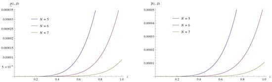
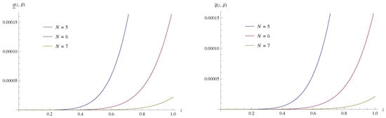
with initial conditions $(\underline{p}(0;\beta ),\overline{p}(0;\beta ))=(\frac{-\beta }{5},\frac{\beta }{5})$, $(\underline{q}(0;\beta ),\overline{q}(0;\beta ))=(\beta ,2-\beta )$. The exact solutions of this problem are $(\underline{p}(z;\beta ),\overline{p}(z;\beta ))=(z^2-\frac{\beta }{5},z^2+\frac{\beta }{5})$ and $(\underline{q}(z;\beta ),\overline{q}(z;\beta ))=(e^{-z}+\beta -1,e^{-z}-\beta +1)$. The approximate solutions obtained by present method have been compared with the exact solutions and shown in the Table 1 and Table 2. Figure 1 and Figure 2 show the absolute errors obtained for $\beta =0.2$. Again the obtained results have been compared with the same by Adomian decomposition method (ADM) (similar approach as given in [13]) and is shown in Table 3.

Table 1. FDTM solution of $(\underline{p}(z;\beta ),\overline{p}(z;\beta ))$ of Example 2 for $N=5$.

	$\mathit{\beta }=0.2$				$\mathit{\beta }=0.8$
z	$\underline{\mathit{p}}(\mathit{z};\mathit{\beta })$		$\overline{\mathit{p}}(\mathit{z};\mathit{\beta })$		$\underline{\mathit{p}}(\mathit{z};\mathit{\beta })$		$\overline{\mathit{p}}(\mathit{z};\mathit{\beta })$
	Appx	Exact	Appx	Exact	Appx	Exact	Appx	Exact
0.1	−0.03	−0.03	0.05	0.05	−0.15	−0.15	0.17	0.17
0.2	$-6.76\times {10}^{-9}$	0	0.0799999	0.08	−0.12	−0.12	0.20	0.20
0.3	0.0499998	0.05	0.13	0.13	−0.07	−0.07	0.249999	0.25
0.4	0.119999	0.12	0.199998	0.20	$-3.94\times {10}^{-7}$	0	0.319997	0.32
0.5	0.209996	0.21	0.289994	0.29	0.0899987	0.09	0.409991	0.41
0.6	0.319989	0.32	0.399984	0.40	0.199997	0.20	0.519977	0.52
0.7	0.449977	0.45	0.529964	0.53	0.329995	0.33	0.649946	0.65
0.8	0.599954	0.60	0.679928	0.68	0.479992	0.48	0.79989	0.80
0.9	0.769915	0.77	0.849866	0.85	0.649988	0.65	0.969794	0.97

Table 2. FDTM solution of $(\underline{q}(z;\beta ),\overline{q}(z;\beta ))$ of Example 2 for $N=5$.

	$\mathit{\beta }=0.2$				$\mathit{\beta }=0.8$
z	$\underline{\mathit{q}}(\mathit{z};\mathit{\beta })$		$\overline{\mathit{q}}(\mathit{z};\mathit{\beta })$		$\underline{\mathit{q}}(\mathit{z};\mathit{\beta })$		$\overline{\mathit{q}}(\mathit{z};\mathit{\beta })$
	Appx	Exact	Appx	Exact	Appx	Exact	Appx	Exact
0.1	0.104837	0.104837	1.70484	1.70484	0.704837	0.704837	1.10484	1.10484
0.2	0.0187307	0.0187308	1.61873	1.61873	0.618731	0.618731	1.01873	1.01873
0.3	−0.0591828	−0.0591818	1.54082	1.54082	0.540817	0.540818	0.940817	0.940818
0.4	−0.129685	−0.12968	1.47031	1.47032	0.470314	0.47032	0.870315	0.87032
0.5	−0.19349	−0.193469	1.40651	1.40653	0.40651	0.406531	0.806512	0.806531
0.6	−0.251248	−0.251188	1.34875	1.34881	0.34875	0.348812	0.748756	0.748812
0.7	−0.303563	−0.303415	1.29644	1.29659	0.296433	0.296585	0.696446	0.696585
0.8	−0.350998	−0.350671	1.24901	1.24933	0.248994	0.249329	0.64902	0.649329
0.9	−0.394085	−0.39343	1.20593	1.20657	0.2059	0.20657	0.60595	0.60657

Figure 1. Absolute error of $(\underline{p}(z;\beta ),\overline{p}(z;\beta ))$ of Example 2 for $\beta =0.2$ and $N=5,6,7$.

Figure 2. Absolute error of $(\underline{q}(z;\beta ),\overline{q}(z;\beta ))$ of Example 2 for $\beta =0.2$ and $N=5,6,7$.

Table 3. Comparison of absolute errors of Example 2 obtained by FDTM and ADM for $N=5$ and $\beta =0.2$.

z	$\underline{\mathit{p}}(\mathit{z};\mathit{\beta })$		$\overline{\mathit{p}}(\mathit{z};\mathit{\beta })$		$\underline{\mathit{q}}(\mathit{z};\mathit{\beta })$		$\overline{\mathit{q}}(\mathit{z};\mathit{\beta })$
	FDTM	ADM	FDTM	ADM	FDTM	ADM	FDTM	ADM
0.1	$1.609\times {10}^{-8}$	$8.146\times {10}^{-3}$	$1.887\times {10}^{-8}$	$5.301\times {10}^{-4}$	$1.439\times {10}^{-9}$	$4.591\times {10}^{-3}$	$1.277\times {10}^{-9}$	$9.775\times {10}^{-4}$
0.2	$6.755\times {10}^{-9}$	$4.304\times {10}^{-3}$	$6.113\times {10}^{-8}$	$3.321\times {10}^{-4}$	$8.652\times {10}^{-8}$	$1.721\times {10}^{-3}$	$8.157\times {10}^{-8}$	$6.750\times {10}^{-4}$
0.3	$2.394\times {10}^{-7}$	$3.210\times {10}^{-3}$	$3.885\times {10}^{-7}$	$5.791\times {10}^{-3}$	$9.726\times {10}^{-7}$	$5.293\times {10}^{-2}$	$9.259\times {10}^{-7}$	$4.726\times {10}^{-3}$
0.4	$1.221\times {10}^{-6}$	$2.819\times {10}^{-2}$	$1.786\times {10}^{-6}$	$4.804\times {10}^{-3}$	$5.391\times {10}^{-6}$	$4.994\times {10}^{-2}$	$5.151\times {10}^{-6}$	$4.702\times {10}^{-3}$
0.5	$4.039\times {10}^{-6}$	$1.922\times {10}^{-2}$	$5.920\times {10}^{-6}$	$2.651\times {10}^{-3}$	$2.028\times {10}^{-5}$	$1.701\times {10}^{-2}$	$1.946\times {10}^{-5}$	$2.680\times {10}^{-3}$
0.6	$1.051\times {10}^{-5}$	$1.464\times {10}^{-2}$	$1.569\times {10}^{-5}$	$1.501\times {10}^{-3}$	$5.976\times {10}^{-5}$	$1.607\times {10}^{-2}$	$5.753\times {10}^{-5}$	$1.658\times {10}^{-3}$
0.7	$2.336\times {10}^{-5}$	$1.451\times {10}^{-2}$	$3.561\times {10}^{-5}$	$1.339\times {10}^{-3}$	$1.486\times {10}^{-4}$	$1.139\times {10}^{-2}$	$1.435\times {10}^{-4}$	$1.638\times {10}^{-3}$
0.8	$4.640\times {10}^{-5}$	$1.049\times {10}^{-2}$	$7.213\times {10}^{-5}$	$1.184\times {10}^{-3}$	$3.269\times {10}^{-4}$	$1.110\times {10}^{-2}$	$3.165\times {10}^{-4}$	$1.620\times {10}^{-3}$
0.9	$8.471\times {10}^{-5}$	$1.654\times {10}^{-1}$	$1.340\times {10}^{-4}$	$3.067\times {10}^{-2}$	$6.541\times {10}^{-4}$	$2.869\times {10}^{-1}$	$6.346\times {10}^{-4}$	$1.604\times {10}^{-2}$

Example 3. 

Let us consider the systems of fuzzy integro-differential Equations (4) and (5) with $h_1\left(z\right)=1,h_2\left(z\right)=e^{-z},$ $a_1=\frac{1}{3},a_2=\frac{1}{2},$ ${\lambda }_1=2,{\lambda }_2=1$, $Z_0=\frac{3}{10}$.

For $0\le z\le 1$, we consider

$$\begin{array}{cc}\hfill \underline{l_1}(z;\beta )=& -\frac{\beta }{3}+\frac{23{\beta }^2}{5}+\frac{1}{4}(\beta +\cos z)\cos \left(\frac{3}{10}-z\right)+\left(\frac{87\beta }{20}-\frac{1}{3}\right)\cos z-\frac{{\cos }^{2}z}{4}+\left(\frac{\beta }{2}-1\right)\sin z\hfill \\ & +\frac{1}{2}\cos z\sin z\hfill \\ \hfill \overline{l_1}(z;\beta )=& \frac{\beta }{3}+\frac{23{\beta }^2}{5}-\frac{\cos z}{3}-\frac{23\beta \cos z}{5}+\frac{\beta }{2}\sin \frac{3}{20}\sin \left(\frac{3}{20}-z\right)-\frac{1}{2}\cos z\sin \left(\frac{3}{20}\right)\sin \left(\frac{3}{20}-z\right)\hfill \\ & -\sin z-\frac{\beta }{2}\sin z+\frac{1}{2}\cos z\sin z\hfill \end{array}$$

$$\begin{array}{cc}\hfill \underline{l_2}(z;\beta )=& \frac{1}{8e\frac{3}{10}}\left(\cos \left(\frac{3}{10}-z\right)\left(8\beta +\sin z\right)-e^{\frac{3}{10}}\cos z\left(3\sin z+24\beta -2\right)\right.\hfill \\ & \left.+\left(8\beta +\sin z\right)\left(e^{\frac{3}{10}}+2\beta -4\beta e^{\frac{3}{10}}-\sin \left(\frac{3}{10}-z\right)-e^{\frac{3}{10}}\sin z\right)\right)\hfill \\ \hfill \overline{l_2}(z;\beta )=& -\beta -4{\beta }^2+\frac{2{\beta }^2}{e^{\frac{3}{10}}}-\frac{\beta \cos (\frac{3}{10}-z)}{e^{\frac{3}{10}}}+\frac{\cos z}{4}+3\beta \cos z+\frac{\beta \sin (\frac{3}{10}-z)}{e^{\frac{3}{10}}}\hfill \\ & +\frac{\sin z}{8}+\frac{3\beta \sin z}{2}-\frac{\beta \sin z}{4e^{\frac{3}{10}}}+\frac{\cos (\frac{3}{10}-z)\sin z}{8e^{\frac{3}{10}}}-\frac{3}{8}\cos z\sin z-\frac{\sin (\frac{3}{10}-z)\sin z}{8e^{\frac{3}{10}}}-\frac{{\sin }^{2}z}{8}\hfill \end{array}$$

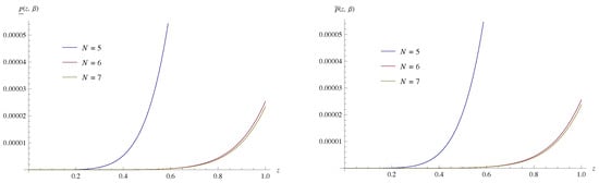
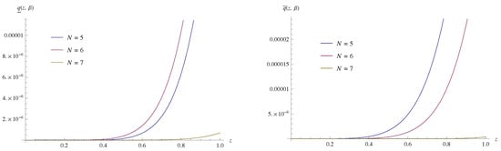
with initial conditions $(\underline{p}(0;\beta ),\overline{p}(0;\beta ))=(1+\beta ,1-\beta )$, $(\underline{q}(0;\beta ),\overline{q}(0;\beta ))=(2\beta ,-2\beta )$. The exact solutions of this problem are $(\underline{p}(z;\beta ),\overline{p}(z;\beta ))=(\cos z-\beta ,\cos z-\beta )$ and $(\underline{q}(z;\beta ),\overline{q}(z;\beta ))=(\frac{1}{4}\sin z+2\beta ,\frac{1}{4}\sin z-2\beta )$. The approximate solutions obtained by present method have been compared with the exact solutions and shown in the Table 4 and Table 5. Figure 3 and Figure 4 show the absolute errors obtained for $\beta =0.1$. Again the obtained results have been compared with the same by ADM (similar approach as given in [13]) and is shown in Table 6.

Table 4. FDTM solution of $(\underline{p}(z,\beta ),\overline{p}(z,\beta ))$ of Example 3 for $N=5$.

	$\mathit{\beta }=0.1$				$\mathit{\beta }=0.9$
z	$\underline{\mathit{p}}(\mathit{z};\mathit{\beta })$		$\overline{\mathit{p}}(\mathit{z};\mathit{\beta })$		$\underline{\mathit{p}}(\mathit{z};\mathit{\beta })$		$\overline{\mathit{p}}(\mathit{z};\mathit{\beta })$
	Appx	Exact	Appx	Exact	Appx	Exact	Appx	Exact
0.1	1.095	1.095	0.895004	0.895004	1.895	1.895	0.0950042	0.0950042
0.2	1.08007	1.08007	0.880067	0.880067	1.88007	1.88007	0.0800667	0.0800666
0.3	1.05534	1.05534	0.855337	0.855336	1.85534	1.85534	0.0553375	0.0553365
0.4	1.02107	1.02106	0.821066	0.821061	1.82106	1.82106	0.0210667	0.021061
0.5	0.977603	0.977583	0.777603	0.777583	1.77759	1.77758	−0.0223958	−0.0224174
0.6	0.925396	0.925336	0.725398	0.725336	1.72537	1.72534	−0.0746	−0.0746644
0.7	0.864995	0.864842	0.664999	0.664842	1.66493	1.66484	−0.134996	−0.135158
0.8	0.797047	0.796707	0.597057	0.596707	1.59690	1.59671	−0.202933	−0.203293
0.9	0.7223	0.72161	0.522318	0.52161	1.52203	1.52161	−0.277663	−0.27839

Table 5. FDTM solution of $(\underline{q}(z;\beta ),\overline{q}(z;\beta ))$ of Example 3 for $N=5$.

	$\mathit{\beta }=0.1$				$\mathit{\beta }=0.9$
z	$\underline{\mathit{q}}(\mathit{z};\mathit{\beta })$		$\overline{\mathit{q}}(\mathit{z};\mathit{\beta })$		$\underline{\mathit{q}}(\mathit{z};\mathit{\beta })$		$\overline{\mathit{q}}(\mathit{z};\mathit{\beta })$
	Appx	Exact	Appx	Exact	Appx	Exact	Appx	Exact
0.1	0.224958	0.224958	−0.175042	−0.175042	1.82496	1.82496	−1.77504	−1.77504
0.2	0.249667	0.249667	−0.150333	−0.150333	1.84967	1.84967	−1.75033	−1.75033
0.3	0.27388	0.27388	−0.12612	−0.12612	1.87388	1.87388	−1.72612	−1.72612
0.4	0.297355	0.297355	−0.102645	−0.102645	1.89735	1.89735	−1.70265	−1.70265
0.5	0.319857	0.319856	−0.0801420	−0.0801436	1.91985	1.91986	−1.68014	−1.68014
0.6	0.341161	0.341161	−0.0588345	−0.0588394	1.94113	1.94116	−1.65884	−1.65884
0.7	0.361057	0.361054	−0.0389333	−0.0389456	1.96099	1.96105	−1.63894	−1.63895
0.8	0.379345	0.379339	−0.0206337	−0.020661	1.9792	1.97934	−1.62065	−1.62066
0.9	0.395847	0.395832	−0.0041126	−0.00416827	1.99558	1.99583	−1.60414	−1.60417

Figure 3. Absolute error of $(\underline{p}(z;\beta ),\overline{p}(z;\beta ))$ of Example 3 for $\beta =0.1$ and $N=5,6,7$.

Figure 4. Absolute error of $(\underline{q}(z;\beta ),\overline{q}(z;\beta ))$ of Example 3 for $\beta =0.1$ and $N=5,6,7$.

Table 6. Comparison of absolute errors of Example 3 obtained by FDTM and ADM for $N=5$ and $\beta =0.1$.

z	$\underline{\mathit{p}}(\mathit{z};\mathit{\beta })$		$\overline{\mathit{p}}(\mathit{z};\mathit{\beta })$		$\underline{\mathit{q}}(\mathit{z};\mathit{\beta })$		$\overline{\mathit{q}}(\mathit{z};\mathit{\beta })$
	FDTM	ADM	FDTM	ADM	FDTM	ADM	FDTM	ADM
0.1	$1.183\times {10}^{-8}$	$6.814\times {10}^{-4}$	$6.034\times {10}^{-9}$	$5.384\times {10}^{-4}$	$9.789\times {10}^{-9}$	$8.369\times {10}^{-4}$	$7.527\times {10}^{-9}$	$5.997\times {10}^{-4}$
0.2	$7.074\times {10}^{-8}$	$1.034\times {10}^{-3}$	$7.641\times {10}^{-8}$	$4.998\times {10}^{-4}$	$1.240\times {10}^{-8}$	$5.559\times {10}^{-4}$	$1.606\times {10}^{-8}$	$3.607\times {10}^{-4}$
0.3	$9.321\times {10}^{-7}$	$2.983\times {10}^{-3}$	$9.658\times {10}^{-7}$	$6.690\times {10}^{-3}$	$1.167\times {10}^{-8}$	$4.801\times {10}^{-3}$	$8.929\times {10}^{-8}$	$4.716\times {10}^{-3}$
0.4	$5.288\times {10}^{-6}$	$2.793\times {10}^{-3}$	$5.475\times {10}^{-6}$	$5.012\times {10}^{-3}$	$1.278\times {10}^{-8}$	$4.053\times {10}^{-3}$	$4.479\times {10}^{-7}$	$4.619\times {10}^{-3}$
0.5	$2.022\times {10}^{-5}$	$2.666\times {10}^{-3}$	$2.091\times {10}^{-5}$	$3.681\times {10}^{-3}$	$1.496\times {10}^{-7}$	$1.862\times {10}^{-3}$	$1.655\times {10}^{-6}$	$2.884\times {10}^{-3}$
0.6	$6.049\times {10}^{-5}$	$1.978\times {10}^{-2}$	$6.242\times {10}^{-5}$	$2.659\times {10}^{-3}$	$6.739\times {10}^{-7}$	$1.674\times {10}^{-3}$	$4.877\times {10}^{-6}$	$2.515\times {10}^{-3}$
0.7	$1.527\times {10}^{-4}$	$1.889\times {10}^{-2}$	$1.572\times {10}^{-4}$	$1.946\times {10}^{-3}$	$2.261\times {10}^{-6}$	$1.488\times {10}^{-2}$	$1.223\times {10}^{-5}$	$1.957\times {10}^{-3}$
0.8	$3.404\times {10}^{-4}$	$1.701\times {10}^{-2}$	$3.500\times {10}^{-4}$	$1.853\times {10}^{-3}$	$6.323\times {10}^{-6}$	$1.211\times {10}^{-2}$	$2.729\times {10}^{-5}$	$1.596\times {10}^{-3}$
0.9	$6.901\times {10}^{-4}$	$1.598\times {10}^{-2}$	$7.083\times {10}^{-4}$	$1.867\times {10}^{-2}$	$1.548\times {10}^{-5}$	$1.186\times {10}^{-2}$	$5.566\times {10}^{-5}$	$2.732\times {10}^{-2}$

6. Conclusions

The system of integro-differential equations in this paper was solved using the fuzzy differential transformation approach, which also produced the findings. The system of integro-differential equations is reduced using the current methods to a system of nonlinear algebraic equations, and this system has been numerically solved. The purpose of the illustrated cases is to show the applicability and validity of the suggested techniques. These examples also show how accurate and effective the current approaches are. Moreover, the presented results have been compared with the results obtained by ADM to manifest the efficiency of the proposed method.

References

- Wazwaz, A.M. Linear and Nonlinear Integral Equations: Methods and Applications; Springer: Beijing, China, 2011. [Google Scholar]
- Wang, H.; Fu, H.M.; Zhang, H.F.; Hu, Z.Q. A practical thermodynamic method to calculate the best glass-forming composition for bulk metallic glasses. Int. J. Nonlinear Sci. Numer. Simul. 2007, 8, 171–178. [Google Scholar] [CrossRef]
- Xu, L.; He, J.H.; Liu, Y. Electrospun nanoporous spheres with Chinese drug. Int. J. Nonlinear Sci. Numer. Simul. 2007, 8, 199–202. [Google Scholar] [CrossRef]
- Sun, F.Z.; Gao, M.; Lei, S.H.; Zhao, Y.B.; Wang, K.; Shi, Y.T.; Wang, N.H. The fractal dimension of the fractal model of dropwise condensation and its experimental study. Int. J. Nonlinear Sci. Numer. Simul. 2007, 8, 211–222. [Google Scholar] [CrossRef]
- Bo, T.L.; Xie, L.; Zheng, X.J. Numerical approach to wind ripple in desert. Int. J. Nonlinear Sci. Numer. Simul. 2007, 8, 223–228. [Google Scholar] [CrossRef]
- Shakeri, F.; Dehghan, M. Solution of a model describing biological species living together using the variational iteration method. Math. Comput. Model. 2008, 48, 685–699. [Google Scholar] [CrossRef]
- Zadeh, L.A. The concept of a linguistic variable and its application to approximate reasoning. Inform. Sci. 1975, 8, 199–249. [Google Scholar] [CrossRef]
- Chang, S.S.L.; Zadeh, L. On fuzzy mapping and control. IEEE Trans. Syst. Man Cybernet. 1972, 2, 30–34. [Google Scholar] [CrossRef]
- Kaleva, O. Fuzzy differential equations. Fuzzy Sets Syst. 1987, 24, 301–317. [Google Scholar] [CrossRef]
- Seikkala, S. On the fuzzy initial value problem. Fuzzy Sets Syst. 1987, 24, 319–330. [Google Scholar] [CrossRef]
- Salahshour, S.; Allahviranloo, T. Application of fuzzy differential transform method for solving fuzzy Volterra integral equations. Appl. Math. Model. 2013, 37, 1016–1024. [Google Scholar] [CrossRef]
- Babolian, E.; Goghary, H.S.; Abbasbandy, S. Numerical solution of linear Fredholm fuzzy integral equations of the second kind by Adomian method. Appl. Math.Comput. 2005, 161, 733–744. [Google Scholar] [CrossRef]
- Younis, M.T.; Al-Hayani, W. Solving fuzzy system of Volterra integro-diofferential equations by using Adomian decomposition method. Eur. J. Pure Appl. Math. 2022, 15, 290–313. [Google Scholar] [CrossRef]
- Molabahrami, A.; Shidfar, A.; Ghyasi, A. An analytical method for solving linear Fredholm fuzzy integral equations of the second kind. Comput. Math. Appl. 2011, 61, 2754–2761. [Google Scholar] [CrossRef]
- Allahviranloo, T.; Hashemzehi, S. The homotopy perturbation method for fuzzy Fredholm integral equations. J. Appl. Math. Islam. Azad Univ. Lahijan 2008, 5, 1–12. [Google Scholar]
- Haq, M.U.; Ullah, A.; Ahmad, S.; Akgul, A. A quantitative approach to nth-order nonlinear fuzzy integro-differential equation. Int. J. Appl. Comput. Math. 2022, 8, 92. [Google Scholar] [CrossRef]
- Kang, S.M.; Iqbal, Z.; Habib, M.; Nazeer, W. Sumudu decomposition method for solving fuzzy integro-differential equations. Axioms 2019, 8, 74. [Google Scholar] [CrossRef]
- Jafarian, A.; Rostami, F.; Golmankhaneh, A.K.; Baleanu, D. Using ANNs Approach for Solving Fractional Order Volterra Integro-differential Equations. Int. J. Comput. Intell. Syst. 2017, 10, 470–480. [Google Scholar] [CrossRef]
- Sahu, P.K.; Ray, S.S. Two dimensional Legendre wavelet method for the numerical solutions of fuzzy integro-differential equations. J. Intell. Fuzzy Syst. 2015, 28, 1271–1279. [Google Scholar] [CrossRef]
- Sahu, P.K.; Ray, S.S. A new Bernoulli wavelet method for accurate solutions of nonlinear fuzzy Hammerstein–Volterra delay integral equations. Fuzzy Sets Syst. 2017, 309, 131–144. [Google Scholar] [CrossRef]
- Allahviranloo, T.; Kiani, N.A.; Motamedi, N. Solving fuzzy differential equations by differential transformation method. Inf. Sci. 2009, 179, 956–966. [Google Scholar] [CrossRef]
- Tang, T.; Xu, X.; Cheng, J. On the spectral methods for Volterra integral equations and the convergence analysis. J. Comput. Math. 2008, 26, 825–837. [Google Scholar]
- Samadi, O.R.N.; Tohodi, E. The spectral method for solving systems of Volterra integral equations. J. Appl. Math. Comput. 2012, 40, 477–497. [Google Scholar] [CrossRef]
- Chen, Y.P.; Tang, T. Spectral methods for weakly singular Volterra integral equations with smooth solutions. J. Comput. Appl. Math. 2009, 233, 938–950. [Google Scholar] [CrossRef]
- Puri, M.L.; Ralescu, D. Differential for fuzzy function. J. Math. Anal. Appl. 1983, 91, 552–558. [Google Scholar] [CrossRef]
- Chalco-Cano, Y.; Román-Flores, H. On new solutions of fuzzy differential equations. Chaos Solitons Fractals 2008, 38, 552–558. [Google Scholar] [CrossRef]
Disclaimer/Publisher’s Note: The statements, opinions and data contained in all publications are solely those of the individual author(s) and contributor(s) and not of MDPI and/or the editor(s). MDPI and/or the editor(s) disclaim responsibility for any injury to people or property resulting from any ideas, methods, instructions or products referred to in the content. |
© 2023 by the authors. Licensee MDPI, Basel, Switzerland. This article is an open access article distributed under the terms and conditions of the Creative Commons Attribution (CC BY) license (https://creativecommons.org/licenses/by/4.0/).