Bayesian Identification Procedure for Triple Seasonal Autoregressive Models

Abstract

Triple seasonal autoregressive (TSAR) models have been introduced to model time series date with three layers of seasonality; however, the Bayesian identification problem of these models has not been tackled in the literature. Therefore, in this paper, we have the objective of filling this gap by presenting a Bayesian procedure to identify the best order of TSAR models. Assuming that the TSAR model errors are normally distributed along with employing three priors, i.e., normal-gamma, Jeffreys’ and g priors, on the model parameters, we derive the marginal posterior distributions of the TSAR model parameters. In particular, we show that the marginal posteriors are multivariate t and gamma distributions for the TSAR model coefficients vector and precision, respectively. Using the marginal posterior distribution of the TSAR model coefficients vector, we present an identification procedure for the TSAR models based on a sequence of t-test of significance. We evaluate the accuracy of the proposed Bayesian identification procedure by conducting an extensive simulation study, followed by a real application to hourly electricity load datasets in six European countries.

1. Introduction

Modeling time series data with multiple seasonalities is a challenging task [1,2,3], and researchers have extended autoregressive moving average (ARMA) models to fit these time series and accommodate multiple seasonalities [4,5,6,7]. Bayesian analysis of seasonal ARMA (SARMA) models and their extensions is difficult to handle since the likelihood function of these time series models is complicated and analytically intractable, which complicates the posterior and predictive analyses. Accordingly, analytical approximations and Markov Chain Monte Carlo (MCMC) methods-based approximations have been introduced in the literature to ease and simplify the Bayesian analysis of these models. In general, the analytical approximations idea is mainly carried out by modifying the posterior and predictive densities of SARMA models to be approximated in standard or closed-form distributions that can be analytically tractable; see, for example, Shaarawy and Broemeling [8], Shaarawy and Ismail [9], Shaarawy and Ali [10]. In addition, the idea of approximations based on MCMC methods is carried out by using one or more of these methods to simulate the available conditional posterior or predictive densities of SARMA models to empirically approximate their corresponding marginal posterior or predictive densities; see, for example, Barnett et al. [11], Vermaak et al. [12], Amin [13].

The Bayesian analysis of single SARMA models is well established in the literature [14], starting from the work of Barnett et al. [11,15], which presents the MCMC methods to develop the Bayesian estimation of seasonal autoregressive (SAR) and ARMA models. In addition, Vermaak et al. [12] used the Metropolis within Gibbs sampling algorithm to propose the Bayesian estimation of SAR models in the field of modeling speech production for voiced sounds. Ismail [16,17] introduced the Gibbs sampler to present the Bayesian analysis of the SAR and seasonal moving average (SMA) models, respectively. On the other hand, Shaarawy and Ali [10] presented the analytical approximation to introduce the Bayesian identification of SAR models. Moreover, Ismail and Amin [18] applied the Gibbs sampler to present the Bayesian inference of SARMA models, and, recently, Amin [19] introduced both a Bayesian estimation and prediction of SARMA models via a Gibbs sampler.

The Bayesian analysis of double seasonal ARMA (DSARMA) models is relatively recent and few works have been presented in the literature. Ismail and Zahran [20] presented the analytical approximations to introduce the Bayesian estimation of double SAR (DSAR) models, and Amin [21] applied the Gibbs sampler to develop the Bayesian estimation of DSARMA models. In addition, Amin [22,23] presented analytical approximations to introduce the Bayesian estimation of DSARMA models and the Bayesian identification of DSAR models, respectively. Moreover, recently, Amin [24,25] presented the Bayesian analysis of DSAR models via the Gibbs sampler. For the time series with three layers of seasonality, none have introduced or discussed their Bayesian analysis, except our recent work of introducing the analytical approximations [13] and the Gibbs sampling algorithm [26] to present the Bayesian estimation of the TSAR models. However, specifying the best TSAR model order, i.e., the TSAR model identification, is the first and an important stage of the Bayesian analysis of these models that needs to be tackled to model high-frequency time series with three layers of seasonality in real applications.

Therefore, our contribution in this paper is to fill this gap by introducing a testing-based Bayesian procedure to identify the best order of TSAR models. Assuming that the TSAR model errors are normally distributed along with employing three priors, i.e., normal-gamma, Jeffreys’ and g priors, on the model parameters, we first derive the marginal posterior distributions of these TSAR model parameters. In particular, we derive the marginal posteriors to be multivariate t and gamma distributions for the TSAR model coefficients vector and precision, respectively. Since the derived marginal posterior distribution of the TSAR model coefficients vector is a multivariate t-distribution, we present an identification procedure for the TSAR models based on a sequence of t-test of significance, which is a simple and easy procedure to be adopted and applied in real applications. We evaluate the accuracy of the proposed Bayesian identification procedure by conducting an extensive simulation study. In addition, we show the applicability of our work on real hourly electricity load time series datasets in six European countries.

The remainder of this paper is structured as follows. The TSAR models are first introduced in Section 2. In Section 3, we discuss the posterior analysis of these TSAR models, followed by the proposed Bayesian identification procedure. We discuss the simulation study setting and results and then present a real application of the proposed Bayesian identification of TSAR models on hourly electricity load time series in six European countries in Section 4. Finally, in Section 5, the paper is concluded.

2. TSAR Models

The time series $\left\{z_t\right\}$ is said to be generated from the zero-mean triple seasonal autoregressive (TSAR) model of order p, $P_1$, $P_2$ and $P_3$, i.e., TSAR(p)($P_1$)${}_{s_1}$($P_2$)${}_{s_2}$($P_3$)${}_{s_3}$, if it has the form:

$${\mathit{\varphi }}_p\left(B\right){\mathbf{\Phi }}_{P_1}\left(B^{s_1}\right){\mathbf{\Pi }}_{P_2}\left(B^{s_2}\right){\mathbf{\Psi }}_{P_3}\left(B^{s_3}\right)z_t={\epsilon }_t,$$

(1)

where $\left\{{\epsilon }_t\right\}$ is a sequence of random errors that are assumed to be identically independently normally distributed with zero mean and unknown precision $\tau$, $s_1$, $s_2$ and $s_3$ are the seasonal periods and B is the back-shift operator defined as $B^r{z}_t=z_{t-r}$.

$${\mathit{\varphi }}_p\left(B\right)=\left(1-{\varphi }_{1}B-{\varphi }_2{B}^2-\cdots -{\varphi }_p{B}^p\right)$$

is the non-seasonal autoregressive operator of order p. The TSAR model (1) has three seasonal autoregressive operators to accommodate the triple seasonal patterns [13], which are:

$${\mathbf{\Phi }}_{P_1}\left(B^{s_1}\right)=\left(1-{\Phi }_1{B}^{s_1}-{\Phi }_2{B}^{2s_1}-\cdots -{\Phi }_{P_1}{B}^{P_1{s}_1}\right),$$

$${\mathbf{\Pi }}_{P_2}\left(B^{s_2}\right)=\left(1-{\Pi }_1{B}^{s_2}-{\Pi }_2{B}^{2s_2}-\cdots -{\Pi }_{P_2}{B}^{P_2{s}_2}\right)$$

and

$${\mathbf{\Psi }}_{P_3}\left(B^{s_3}\right)=\left(1-{\Psi }_1{B}^{s_3}-{\Psi }_2{B}^{2s_3}-\cdots -{\Psi }_{P_3}{B}^{P_3{s}_3}\right)$$

with orders $P_1,P_2$ and $P_3$, respectively.

The non-seasonal and seasonal autoregressive coefficients are $\mathit{\varphi }={\left({\varphi }_1,{\varphi }_2,\cdots ,{\varphi }_p\right)}^T$, $\mathbf{\Phi }={\left({\Phi }_1,{\Phi }_2,\cdots ,{\Phi }_{P_1}\right)}^T$, $\mathbf{\Pi }={\left({\Pi }_1,{\Pi }_2,\cdots ,{\Pi }_{P_2}\right)}^T$ and $\mathbf{\Psi }={\left({\Psi }_1,{\Psi }_2,\cdots ,{\Psi }_{P_3}\right)}^T$, respectively.

Using the summation notation, we can expand and simplify the compact form of the TSAR model (1) to be:

$$\begin{array}{ccc}\hfill z_t& =& \sum _{i=1}^p{\varphi }_i{z}_{t-i}+\sum _{j=1}^{P_1}{\Phi }_j{z}_{t-j{s}_1}+\sum _{m=1}^{P_2}{\Pi }_m{z}_{t-m{s}_2}+\sum _{k=1}^{P_3}{\Psi }_k{z}_{t-k{s}_3}-\sum _{i=1}^p\sum _{j=1}^{P_1}{\varphi }_i{\Phi }_j{z}_{t-i-j{s}_1}-\hfill \\ & & \sum _{i=1}^p\sum _{m=1}^{P_2}{\varphi }_i{\Pi }_m{z}_{t-i-m{s}_2}-\sum _{i=1}^p\sum _{k=1}^{P_3}{\varphi }_i{\Psi }_k{z}_{t-i-k{s}_3}-\sum _{j=1}^{P_1}\sum _{m=1}^{P_2}{\Phi }_j{\Pi }_m{z}_{t-j{s}_1-m{s}_2}-\hfill \\ & & \sum _{j=1}^{P_1}\sum _{k=1}^{P_3}{\Phi }_j{\Psi }_k{z}_{t-j{s}_1-k{s}_3}-\sum _{m=1}^{P_2}\sum _{k=1}^{P_3}{\Pi }_m{\Psi }_k{z}_{t-m{s}_2-k{s}_3}+\sum _{i=1}^p\sum _{j=1}^{P_1}\sum _{m=1}^{P_2}{\varphi }_i{\Phi }_j{\Pi }_m{z}_{t-i-j{s}_1-m{s}_2}+\hfill \\ & & \sum _{i=1}^p\sum _{j=1}^{P_1}\sum _{k=1}^{P_3}{\varphi }_i{\Phi }_j{\Psi }_k{z}_{t-i-j{s}_1-k{s}_3}+\sum _{i=1}^p\sum _{m=1}^{P_2}\sum _{k=1}^{P_3}{\varphi }_i{\Pi }_m{\Psi }_k{z}_{t-i-m{s}_2-k{s}_3}+\hfill \\ & & \sum _{j=1}^{P_1}\sum _{m=1}^{P_2}\sum _{k=1}^{P_3}{\Phi }_j{\Pi }_m{\Psi }_k{z}_{t-j{s}_1-m{s}_2-k{s}_3}-\sum _{i=1}^p\sum _{j=1}^{P_1}\sum _{m=1}^{P_2}\sum _{k=1}^{P_3}{\varphi }_i{\Phi }_j{\Pi }_m{\Psi }_k{z}_{t-i-j{s}_1-m{s}_2-k{s}_3}+{\epsilon }_t.\hfill \end{array}$$

(2)

In addition, we can write the matrix form of the TSAR model as:

$$\begin{array}{ccc}\hfill \mathbf{Z}& =& X\beta +\epsilon ,\hfill \end{array}$$

(3)

where $\mathbf{Z}={\left(z_1,z_2,\cdots ,z_n\right)}^T$ is the vector of observed time series, $\epsilon ={\left({\epsilon }_1,{\epsilon }_2,\dots ,{\epsilon }_n\right)}^T$ is the vector of unobserved model errors, X is an $n\times q$ design matrix, i.e., $q=(1+p)(1+P_1)(1+P_2)(1+P_3)-1$, with the tth row:

$$\begin{array}{ccc}\hfill X_t& =& \left(z_{t-1},\dots ,z_{t-p},z_{t-s_1},z_{t-s_1-1},\dots ,z_{t-s_1-p},\dots ,z_{t-P_1{s}_1},z_{t-P_1{s}_1-1},\dots ,z_{t-P_1{s}_1-p},z_{t-s_2},\right.\hfill \\ & & z_{t-s_2-1},\dots ,z_{t-s_2-p},z_{t-s_2-s_1},z_{t-s_2-s_1-1},\dots ,z_{t-s_2-s_1-p},\dots ,z_{t-s_2-P_1{s}_1},z_{t-s_2-P_1{s}_1-1},\hfill \\ & & \dots ,z_{t-s_2-P_1{s}_1-p},\dots ,z_{t-P_2{s}_2},z_{t-P_2{s}_2-1},\dots ,z_{t-P_2{s}_2-p},z_{t-P_2{s}_2-s_1},z_{t-P_2{s}_2-s_1-1},\dots ,\hfill \\ & & z_{t-P_2{s}_2-s_1-p},\dots ,z_{t-P_2{s}_2-P_1{s}_1},z_{t-P_2{s}_2-P_1{s}_1-1},\dots ,z_{t-P_2{s}_2-P_1{s}_1-p},z_{t-s_3},z_{t-s_3-1},\dots ,\hfill \\ & & z_{t-s_3-p},z_{t-s_3-s_1},z_{t-s_3-s_1-1},\dots ,z_{t-s_3-s_1-p},\dots ,z_{t-s_3-P_1{s}_1},z_{t-s_3-P_1{s}_1-1},\dots ,z_{t-s_3-P_1{s}_1-p},\hfill \\ & & z_{t-s_3-s_2},z_{t-s_3-s_2-1},\dots ,z_{t-s_3-s_2-p},z_{t-s_3-s_2-s_1},z_{t-s_3-s_2-s_1-1},\dots ,z_{t-s_3-s_2-s_1-p},\dots ,\hfill \\ & & z_{t-s_3-P_1{s}_1-s_2},z_{t-s_3-P_1{s}_1-s_2-1},\dots ,z_{t-s_3-P_1{s}_1-s_2-p},\dots ,z_{t-s_3-P_2{s}_2},z_{t-s_3-P_2{s}_2-1},\dots ,\hfill \\ & & z_{t-s_3-P_2{s}_2-p},z_{t-s_3-s_1-P_2{s}_2},z_{t-s_3-s_1-P_2{s}_2-1},\dots ,z_{t-s_3-s_1-P_2{s}_2-p},\dots ,z_{t-s_3-P_1{s}_1-P_2{s}_2},\hfill \\ & & z_{t-s_3-P_1{s}_1-P_2{s}_2-1},\dots ,z_{t-s_3-P_1{s}_1-P_2{s}_2-p},\dots ,z_{t-P_3{s}_3},z_{t-P_3{s}_3-1},\dots ,z_{t-P_3{s}_3-p},\hfill \\ & & z_{t-P_3{s}_3-s_1},z_{t-P_3{s}_3-s_1-1},\dots ,z_{t-P_3{s}_3-s_1-p},\dots ,z_{t-P_3{s}_3-P_1{s}_1},z_{t-P_3{s}_3-P_1{s}_1-1},\dots ,\hfill \\ & & z_{t-P_3{s}_3-P_1{s}_1-p},z_{t-s_2},z_{t-P_3{s}_3-s_2-1},\dots ,z_{t-P_3{s}_3-s_2-p},z_{t-P_3{s}_3-s_1-s_2},z_{t-P_3{s}_3-s_1-s_2-1},\dots ,\hfill \\ & & z_{t-P_3{s}_3-s_1-s_2-p},\dots ,z_{t-P_3{s}_3-P_1{s}_1-s_2},z_{t-P_3{s}_3-P_1{s}_1-s_2-1},\dots ,z_{t-P_3{s}_3-P_1{s}_1-s_2-p},\dots ,\hfill \\ & & z_{t-P_3{s}_3-P_2{s}_2},z_{t-P_3{s}_3-P_2{s}_2-1},\dots ,z_{t-P_3{s}_3-P_2{s}_2-p},z_{t-P_3{s}_3-s_1-P_2{s}_2},z_{t-P_3{s}_3-s_1-P_2{s}_2-1},\dots ,\hfill \\ & & \left.z_{t-P_3{s}_3-s_1-P_2{s}_2-p},\dots ,z_{t-P_3{s}_3-P_1{s}_1-P_2{s}_2},z_{t-P_3{s}_3-P_1{s}_1-P_2{s}_2-1},\dots ,z_{t-P_3{s}_3-P_1{s}_1-P_2{s}_2-p}\right),\hfill \end{array}$$

(4)

and $\beta$ is the vector of TSAR model coefficients given as:

$$\begin{array}{ccc}\hfill \beta & =& \left({\varphi }_1,\dots ,{\varphi }_p,{\Phi }_1,-{\varphi }_1{\Phi }_1,\dots ,-{\varphi }_p{\Phi }_1,\dots ,{\Phi }_{P_1},-{\varphi }_1{\Phi }_{P_1},\dots ,-{\varphi }_p{\Phi }_{P_1},{\Pi }_1,-{\varphi }_1{\Pi }_1,\dots ,-{\varphi }_p{\Pi }_1,\right.\hfill \\ & & -{\Phi }_1{\Pi }_1,{\varphi }_1{\Phi }_1{\Pi }_1,\dots ,{\varphi }_p{\Phi }_1{\Pi }_1,\dots ,-{\Phi }_{P_1}{\Pi }_1,{\varphi }_1{\Phi }_{P_1}{\Pi }_1,\dots ,{\varphi }_p{\Phi }_{P_1}{\Pi }_1,\dots ,{\Pi }_{P_2},-{\varphi }_1{\Pi }_{P_2},\hfill \\ & & \dots ,-{\varphi }_p{\Pi }_{P_2},-{\Phi }_1{\Pi }_{P_2},{\varphi }_1{\Phi }_1{\Pi }_{P_2},\dots ,{\varphi }_p{\Phi }_1{\Pi }_{P_2},\dots ,-{\Phi }_{P_1}{\Pi }_{P_2},{\varphi }_1{\Phi }_{P_1}{\Pi }_{P_2},\dots ,{\varphi }_p{\Phi }_{P_1}{\Pi }_{P_2},\hfill \\ & & {\Psi }_1,-{\varphi }_1{\Psi }_1,\dots ,-{\varphi }_p{\Psi }_1,-{\Phi }_1{\Psi }_1,{\varphi }_1{\Phi }_1{\Psi }_1,\dots ,{\varphi }_p{\Phi }_1{\Psi }_1,\dots ,-{\Phi }_{P_1}{\Psi }_1,{\varphi }_1{\Phi }_{P_1}{\Psi }_1,\dots ,{\varphi }_p{\Phi }_{P_1}{\Psi }_1,\hfill \\ & & -{\Pi }_1{\Psi }_1,{\varphi }_1{\Pi }_1{\Psi }_1,\dots ,{\varphi }_p{\Pi }_1{\Psi }_1,{\Phi }_1{\Pi }_1{\Psi }_1,-{\varphi }_1{\Phi }_1{\Pi }_1{\Psi }_1,\dots ,-{\varphi }_p{\Phi }_1{\Pi }_1{\Psi }_1,\dots ,{\Phi }_{P_1}{\Pi }_1{\Psi }_1,\hfill \\ & & -{\varphi }_1{\Phi }_{P_1}{\Pi }_1{\Psi }_1,\dots ,-{\varphi }_p{\Phi }_{P_1}{\Pi }_1{\Psi }_1,\dots ,-{\Pi }_{P_2}{\Psi }_1,{\varphi }_1{\Pi }_{P_2}{\Psi }_1,\dots ,{\varphi }_p{\Pi }_{P_2}{\Psi }_1,{\Phi }_1{\Pi }_{P_2}{\Psi }_1,\hfill \\ & & -{\varphi }_1{\Phi }_1{\Pi }_{P_2}{\Psi }_1,\dots ,-{\varphi }_p{\Phi }_1{\Pi }_{P_2}{\Psi }_1,\dots ,{\Phi }_{P_1}{\Pi }_{P_2}{\Psi }_1,-{\varphi }_1{\Phi }_{P_1}{\Pi }_{P_2}{\Psi }_1,\dots ,-{\varphi }_p{\Phi }_{P_1}{\Pi }_{P_2}{\Psi }_1,\hfill \\ & & {\Psi }_{P_3},-{\varphi }_1{\Psi }_{P_3},\dots ,-{\varphi }_p{\Psi }_{P_3},-{\Phi }_1{\Psi }_{P_3},{\varphi }_1{\Phi }_1{\Psi }_{P_3},\dots ,{\varphi }_p{\Phi }_1{\Psi }_{P_3},\dots ,-{\Phi }_{P_1}{\Psi }_{P_3},{\varphi }_1{\Phi }_{P_1}{\Psi }_{P_3},\dots ,\hfill \\ & & {\varphi }_p{\Phi }_{P_1}{\Psi }_{P_3},-{\Pi }_1{\Psi }_{P_3},{\varphi }_1{\Pi }_1{\Psi }_{P_3},\dots ,{\varphi }_p{\Pi }_1{\Psi }_{P_3},{\Phi }_1{\Pi }_1{\Psi }_{P_3},-{\varphi }_1{\Phi }_1{\Pi }_1{\Psi }_{P_3},\dots ,-{\varphi }_p{\Phi }_1{\Pi }_1{\Psi }_{P_3},\hfill \\ & & \dots ,{\Phi }_{P_1}{\Pi }_1{\Psi }_{P_3},-{\varphi }_1{\Phi }_{P_1}{\Pi }_1{\Psi }_{P_3},\dots ,-{\varphi }_p{\Phi }_{P_1}{\Pi }_1{\Psi }_{P_3},\dots ,-{\Pi }_{P_2}{\Psi }_{P_3},{\varphi }_1{\Pi }_{P_2}{\Psi }_{P_3},\dots ,\hfill \\ & & {\varphi }_p{\Pi }_{P_2}{\Psi }_{P_3},{\Phi }_1{\Pi }_{P_2}{\Psi }_{P_3},-{\varphi }_1{\Phi }_1{\Pi }_{P_2}{\Psi }_{P_3},\dots ,-{\varphi }_p{\Phi }_1{\Pi }_{P_2}{\Psi }_{P_3},\dots ,{\Phi }_{P_1}{\Pi }_{P_2}{\Psi }_{P_3},\hfill \\ & & {\left.-{\varphi }_1{\Phi }_{P_1}{\Pi }_{P_2}{\Psi }_{P_3},\dots ,-{\varphi }_p{\Phi }_{P_1}{\Pi }_{P_2}{\Psi }_{P_3}\right)}^T.\hfill \end{array}$$

(5)

It has to be noted that, when the TSAR model orders p, $P_1$, $P_2$ and $P_3$ are unknown, the design matrix X in the TSAR model (3) is a function of p, $P_1$, $P_2$ and $P_3$, which complicates the posterior analysis of these models and shows the importance of our work in this paper.

3. Posterior Analysis and Proposed Identification Procedure for TSAR Models

We can obtain the posterior distribution of the TSAR model parameters by simply combining the prior distribution of these model parameters with the likelihood function of time series data $\left\{z_t\right\}$ [27]. First, for the likelihood function of observed time series data $\left\{z_t\right\}$, assuming the random errors $\left\{{\epsilon }_t\right\}$ of the TSAR model (3) are normally distributed and using a straightforward transformation from the model errors $\epsilon$ to $\mathbf{Z}$ [28], the conditional likelihood function on the first $P^{★}$ initial values, i.e., $P^{★}$ = $P_3{s}_3+P_2{s}_2+P_1{s}_1+p$, can be given as:

$$\begin{array}{ccc}\hfill L(\beta ,\tau \mid \mathbf{Z})& \propto & {\tau }^{\frac{n-P^{★}}{2}}exp\left\{-\frac{\tau }{2}{\epsilon }^T\epsilon \right\},\hfill \\ & \propto & {\tau }^{\frac{n-P^{★}}{2}}exp\left\{-\frac{\tau }{2}{\left(\mathbf{Z}-X\beta \right)}^T\left(\mathbf{Z}-X\beta \right)\right\}.\hfill \end{array}$$

(6)

On the other hand, for the prior specification of TSAR model parameters $\beta$ and $\tau$, we assume the products of non-seasonal and seasonal coefficients to be free coefficients and consider three prior distributions: normal-gamma, g and Jeffreys’ priors. Suppose that $\tau \sim G(\frac{\nu }{2},\frac{\lambda }{2})$ and $\beta \sim N_{p^{★}}({\mu }_{\beta },{\tau }^{-1}{\Sigma }_{\beta })$; the normal-gamma prior of $\beta$ and $\tau$ can be written as:

$$\begin{array}{ccc}\hfill {\zeta }_n\left(\beta ,\tau \right)& \propto & {\tau }^{\left(\frac{\nu +q}{2}-1\right)}exp\left\{-\frac{\tau }{2}\left[\lambda +{\left(\beta -{\mu }_{\beta }\right)}^T{\Sigma }_{\beta }^{-1}\left(\beta -{\mu }_{\beta }\right)\right]\right\},\hfill \end{array}$$

(7)

where the parameters ${\mu }_{\beta },{\Sigma }_{\beta },\nu$ and $\lambda$ are hyper-parameters of the normal-gamma prior that need to be estimated to conduct the Bayesian analysis.

In addition, we employ the g prior for the parameters $\beta$ and $\tau$ with the objective of simplifying the elicitation of covariances of these parameters. Thus, the g prior of $\beta$ and $\tau$ can be given as:

$$\begin{array}{ccc}\hfill {\zeta }_g\left(\beta ,\tau \right)& \propto & {\tau }^{(\frac{q}{2}-1)}exp\left\{-\frac{g\tau }{2}{\left(\beta -\overline{\beta }\right)}^T\left(X^{T}X\right)\left(\beta -\overline{\beta }\right)\right\},\hfill \end{array}$$

(8)

where g is a hyper-parameter that might be specified as a function of the size of time series n and the number of model coefficients; for more details about how to set the g hyper-parameter value, see Fernandez et al. [29].

In case no or little information is available about the model parameters $\beta$ and $\tau$, Jeffreys’ prior can be employed, and it is given as:

$$\begin{array}{ccc}\hfill {\zeta }_j\left(\beta ,\tau \right)& \propto & {\tau }^{-1},\tau >0\hfill \end{array}$$

(9)

In order to obtain the joint posterior of $\beta$ and $\tau$, we multiply the likelihood function given in (6) by each one of the above-given three prior distributions in (7)–(9). Following this Bayesian rule and for the normal-gamma prior (7), the joint posterior of $\beta$ and $\tau$ is given as:

$$\begin{array}{ccc}\hfill {\zeta }_n\left(\beta ,\tau \mid \mathbf{Z}\right)& \propto & {\tau }^{\left(\frac{n-P^{★}+\nu +q}{2}-1\right)}exp\left\{-\frac{\tau }{2}\left[\lambda +{\left(\beta -{\mu }_{\beta }\right)}^T\right.\right.\hfill \\ & & \left.\left.{\Sigma }_{\beta }^{-1}\left(\beta -{\mu }_{\beta }\right)+{\left(\mathbf{Z}-X\beta \right)}^T\left(\mathbf{Z}-X\beta \right)\right]\right\}.\hfill \end{array}$$

(10)

In addition, for the g prior (8), the joint posterior of $\beta$ and $\tau$ is given as:

$$\begin{array}{ccc}\hfill {\zeta }_g\left(\beta ,\tau \mid \mathbf{Z}\right)& \propto & {\tau }^{\left(\frac{n-P^{★}+q}{2}-1\right)}exp\left\{-\frac{\tau }{2}\left[{\left(\beta -\overline{\beta }\right)}^T\left(g{X}^{T}X\right)\right.\right.\hfill \\ & & \left.\left.\left(\beta -\overline{\beta }\right)+{\left(\mathbf{Z}-X\beta \right)}^T\left(\mathbf{Z}-X\beta \right)\right]\right\}.\hfill \end{array}$$

(11)

Moreover, for Jeffreys’ prior (9), the joint posterior of $\beta$ and $\tau$ is given as:

$$\begin{array}{ccc}\hfill {\zeta }_j\left(\beta ,\tau \mid \mathbf{Z}\right)& \propto & {\tau }^{\left(\frac{n-P^{★}}{2}-1\right)}exp\left\{-\frac{\tau }{2}{\left(\mathbf{Z}-X\beta \right)}^T\left(\mathbf{Z}-X\beta \right)\right\}.\hfill \end{array}$$

In our previous work [13], we derived from the joint posteriors in (10)–(12) the marginal posteriors of the TSAR model coefficients vector $\beta$ and precision $\tau$, and we summarize these results in the following theorem and two corollaries.

Theorem 1. 

Given the conditional likelihood function (6) and the normal-gamma prior of β and τ (7), the marginal posterior of the TSAR model coefficients vector β is a multivariate t-distribution with the degrees of freedom $v_n=(n+\nu -P^{★})$, mean vector ${\mu }_n=A_n^{-1}{B}_n$ and dispersion matrix $V_n=\frac{C_n}{v_n-2}{A}_n^{-1}$, and the marginal posterior of the TSAR model precision τ is a gamma distribution with the two parameters $\frac{v_n}{2}$ and $\frac{C_n}{2}$, where $A_n^{-1}={(X^{T}X+{\Sigma }_{\varphi }^{-1})}^{-1}$, $B_n=(X^T\mathbf{Z}+{\Sigma }_{\varphi }^{-1}{\mu }_{\varphi })$ and $C_n=[{\mathbf{Z}}^T\mathbf{Z}+\lambda +{\mu }_{\varphi }^T{\Sigma }_{\varphi }^{-1}{\mu }_{\varphi }-B_n^T{A}_n^{-1}{B}_n]$.

Proof. 

We multiply the conditional likelihood function (6) of observed time series data $\left\{y_t\right\}$ by the normal-gamma prior of $\beta$ and $\tau$ (7) to obtain the joint posterior of $\beta$ and $\tau$ as given in Equation (10). We then integrate (10) over $\tau$ and complete the square with respect to $\beta$, leading to the given marginal posterior of the TSAR model coefficients vector $\beta$. On the other hand, we complete the square in the exponent of (10) with respect to $\beta$ and then integrate over $\beta$, leading to the given marginal posterior of the TSAR model precision $\tau$.

The following two corollaries are special cases of Theorem 1 when little or no information is available a priori about the TSAR model parameters, since we employ the g and Jeffreys’ priors to obtain the marginal posteriors of the TSAR model coefficients vector $\beta$ and precision $\tau$ to also be the multivariate t and gamma distributions, respectively, with different parameters. □

Corollary 1. 

Given the conditional likelihood function (6) and the g prior of β and τ (8), the marginal posterior of the model TSAR coefficients vector β is a multivariate t-distribution with the degrees of freedom $v_g=(n-P^{★})$, mean vector ${\mu }_g=A_g^{-1}{B}_g$ and dispersion matrix $V_g=\frac{C_g}{v_g-2}{A}_g^{-1}$, and the marginal posterior of the TSAR model precision τ is a gamma distribution with the two parameters $\frac{v_g}{2}$ and $\frac{C_g}{2}$, where $A_g^{-1}={\left((g+1)X^{T}X\right)}^{-1}$, $B_g=(X^T\mathbf{Z}+g\left(X^{T}X\right)\overline{\beta })$ and $C_g=[{\mathbf{Z}}^T\mathbf{Z}+g{\overline{\beta }}^T\left(X^{T}X\right)\overline{\beta }-B_g^T{A}_g^{-1}{B}_g]$.

Proof. 

We set $\lambda =\nu =0$, ${\mu }_{\beta }=\overline{\beta }$ and ${\Sigma }_{\beta }^{-1}=g{X}^{T}X$, then directly it follows from Theorem 1. □

Corollary 2. 

Given the conditional likelihood function (6) and Jeffreys’ prior of β and τ (9), the marginal posterior of the TSAR model coefficients vector β is a multivariate t-distribution with the degrees of freedom $v_j=(n-P^{★}-q)$, mean vector ${\mu }_j=A_j^{-1}{B}_j$, and dispersion matrix $V_j=\frac{C_j}{v_j-2}{A}_j^{-1}$, and the marginal posterior of the TSAR model precision τ is a gamma distribution with the two parameters $\frac{v_j}{2}$ and $\frac{C_j}{2}$, where $A_j^{-1}={\left(X^{T}X\right)}^{-1}$, $B_j=X^T\mathbf{Z}$, and $C_j=[{\mathbf{Z}}^T\mathbf{Z}-B_j^T{A}_j^{-1}{B}_j]$.

Proof. 

We set $\lambda =0$, ${\Sigma }_{\beta }^{-1}=\mathbf{0}$, and $\nu =-q$; then, directly, it follows from Theorem 1. □

It is important to mention that an interesting property of the multivariate t-distribution of a given vector $\mathit{X}$ is that each single component of this vector $\mathit{X}$ has a univariate t-distribution and also any subvector of this vector $\mathit{X}$ also has a multivariate t-distribution [30]. Accordingly, using Theorem 1 and Corollaries 1 and 2, the marginal posterior of each one of the TSAR model coefficients vectors $\mathit{\varphi },\mathbf{\Phi },\mathbf{\Pi }$ and $\mathbf{\Psi }$ is a multivariate t-distribution, and the marginal posterior of any single component of each one of them has a univariate t-distribution.

Based on the derived marginal posterior of the TSAR model coefficients, we propose a Bayesian identification procedure to identify the best value of the TSAR model order by first assuming that the maximum values of the TSAR model order p, $P_1$, $P_2$ and $P_3$ are known and given as $k_1$, $k_2$, $k_3$ and $k_4$, respectively. We then consider the following testing scheme as follows:

• Test:

  $$H_0^{(4,1)}:{\Psi }_{k_4}=0\mathrm{against}{H}_1^{(4,1)}:{\Psi }_{k_4}\ne 0,$$

  using the marginal posterior of the coefficient ${\Psi }_{k_4}$, which is a univariate t-distribution.
• If $H_0^{(4,1)}$ is rejected, then the identified value for $P_3$ is $P_3^{*}=k_4$. Otherwise, test:

  $$H_0^{(4,2)}:{\Psi }_{k_4-1}={\Psi }_{k_4}=0\mathrm{against}{H}_1^{(4,2)}:{\Psi }_{k_4-1}\ne 0\mathrm{or}{\Psi }_{k_4}\ne 0,$$

  using the marginal posterior of the coefficients $({\Psi }_{k_4-1},{\Psi }_{k_4})$, which is a multivariate t-distribution.
• Continue executing this sequence of t-test of significance until the null hypothesis $H_0^{(4,i_4)}:{\Psi }_{k_4-i_4+1}=\cdots ={\Psi }_{k_4}=0$ is rejected, and then the identified value for $P_3$ is $P_3^{*}=k_4-i_4+1$, where $0\le P_3^{*}\le k_4$.
• Test:

  $$H_0^{(3,1)}:{\Pi }_{k_3}={\Psi }_{k_4-i_4+2}=\cdots ={\Psi }_{k_4}=0\mathrm{against}$$

  $$H_1^{(3,1)}:{\Pi }_{k_3}\ne 0\mathrm{or}{\Psi }_{k_4-i_4+2}\ne 0\mathrm{or}\dots \mathrm{or}{\Psi }_{k_4}\ne 0,$$

  using the marginal posterior of the coefficients $({\Pi }_{k_3},{\Psi }_{k_4-i_4+2},\dots ,{\Psi }_{k_4})$, which is a multivariate t-distribution.
• If $H_0^{(3,1)}$ is rejected, then the identified value for $P_2$ is $P_2^{*}=k_3$. Otherwise, test:

  $$H_0^{(3,2)}:{\Pi }_{k_3-1}={\Pi }_{k_3}={\Psi }_{k_4-i_4+2}=\cdots ={\Psi }_{k_4}=0\mathrm{against}$$

  $$H_1^{(3,2)}:{\Pi }_{k_3-1}\ne 0\mathrm{or}{\Pi }_{k_3}\ne 0\mathrm{or}{\Psi }_{k_4-i_4+2}\ne 0\mathrm{or}\dots \mathrm{or}{\Psi }_{k_4}\ne 0,$$

  using the marginal posterior of the coefficients $({\Pi }_{k_3-1},{\Pi }_{k_3},{\Psi }_{k_4-i_4+2},\dots ,{\Psi }_{k_4})$, which is a multivariate t-distribution.
• Continue executing this sequence of t-test of significance until the null hypothesis $H_0^{(3,i_3)}:{\Pi }_{k_3-i_3+1}=\cdots ={\Pi }_{k_3}={\Psi }_{k_4-i_4+1}=\cdots ={\Psi }_{k_4}=0$ is rejected, and then the identified value for $P_2$ is $P_2^{*}=k_3-i_3+1$, where $0\le P_2^{*}\le k_3$.
• In the same way, run sequences of t-test of significance for the TSAR model coefficients vectors $\mathit{\varphi }$ and $\mathbf{\Phi }$ until the null hypotheses are rejected, and then the identified values for p and $P_1$ are $0\le p^{*}=k_1-i_1+1\le k_1$ and $0\le P_1^{*}=k_2-i_2+1\le k_2$, respectively.

The outcome of this testing scheme is the values $p^{*}$, $P_1^{*}$, $P_2^{*}$ and $P_3^{*}$ as the best value for the TSAR model order p, $P_1$, $P_2$ and $P_3$, respectively.

An important point that we have to mention here is related to the computational challenge of applying the proposed Bayesian identification procedure. Indeed, capturing triple seasonality requires observing time series under study for long time, which results in time series with a very large sample size that can be considered as big time series data. For example, observing the hourly electricity load for four years results in a time series of size $n\approx$ 35,000. As is known, analyzing big time series data requires a high computational cost, especially when the analysis is conducted using interpreter software.

4. Simulation Study and Real Application

In this section, we evaluate the accuracy of the proposed Bayesian identification for TSAR models by conducting an extensive simulation study, and then we show the applicability of the proposed Bayesian identification procedure on real time series datasets of electricity load in six European countries that have three layers of seasonality.

4.1. Simulation Study

In this simulation study, we evaluate the accuracy of the proposed Bayesian identification procedure for TSAR models by covering different seasonality patterns with different data types and sample sizes. We generate 500 time series datasets of size n (from 3000 to 6000 with an increment of 1000 observations) from five TSAR models, and the design of these TSAR models and the true parameters values are presented in Table 1. As it can be seen from this table that the seasonal periods for gthe enerated time series are $s_1$ = 12, $s_2$ = 60 and $s_3$ = 600, and since the time series size has to be greater than $k_4{s}_3+k_3{s}_2+k_2{s}_1+k_1$, it is justified for our selection for the minimum value of the time series size n to be 3000.

Table 1. Simulation design.

TSAR Model	${\mathit{\varphi }}_1$	${\mathit{\varphi }}_2$	${\mathbf{\Phi }}_1$	${\mathbf{\Phi }}_2$	${\mathbf{\Pi }}_1$	${\mathbf{\Pi }}_2$	${\mathbf{\Psi }}_1$	$\mathit{\tau }$
I.   (1)(1)${}_{12}$(1)${}_{60}$(1)${}_{600}$	0.5		0.4		0.5		0.4	1.0
II.  (2)(1)${}_{12}$(1)${}_{60}$(1)${}_{600}$	0.6	0.3	0.9		−0.8		0.7	1.0
III. (1)(2)${}_{12}$(1)${}_{60}$(1)${}_{600}$	0.9		0.5	−0.4	0.9		0.8	1.0
IV. (2)(2)${}_{12}$(1)${}_{60}$(1)${}_{600}$	0.6	0.3	0.5	−0.4	−0.9		0.8	1.0
V.  (2)(2)${}_{12}$(2)${}_{60}$(1)${}_{600}$	0.6	−0.3	0.5	0.4	0.7	−0.4	0.6	1.0

After obtaining the 500 time series datasets from each one of these five TSAR models with different sizes, we apply the proposed Bayesian identification procedure to identify the best value for the TSAR model order as follows.

• First, we assume that the maximum values of the model order are $k_1=k_2=k_3=k_4=3$, since the maximum order value in the simulated TSAR models is not more than two.
• Second, we employ different priors for the model parameters $\beta$ and $\tau$ in order to evaluate the robustness or sensitivity to prior specification. In particular, we employ Jeffreys’ prior and g prior with five values for the hyper-parameter g, i.e., $g_1=1/n$, $g_2=q/n$, $g_3=\sqrt{1/n}$, $g_4=\sqrt{q/n}$ and $g_5=ln(q+1)/ln\left(n\right)$.
• Third, for each time series, we execute the proposed testing scheme in Section 3 using the marginal posterior of the TSAR model coefficients resulting from the employed priors, and the outcome of this testing scheme is the identified TSAR model order, i.e., $p^{*}$, $P_1^{*}$, $P_2^{*}$ and $P_3^{*}$.

For all the generated time series datasets, we obtain the percentage of correctly identified true TSAR models by simply comparing the identified TSAR order obtained from the testing scheme with the true values of p, $P_1$, $P_2$ and $P_3$ employed to generate the given time series.

In order to explain how the proposed Bayesian identification procedure works to identify the best value of the TSAR model order, we present the results of the testing scheme for only one generated time series with $n=3000$ from TSAR Model I in Table 2. In this table, we present the null hypothesis, p-value calculated from the t distribution and whether the status of the null hypothesis is rejected or not using a 5% significance level for each test. It is worth noting that using the 5% significance level for each test does not guarantee that the overall significance level of the testing scheme equals 0.05, and indeed it is difficult to determine the overall significance level; for more discussion about this point, see, for example, Lütkepohl [31]. The results of the simulation study for all TSAR models are presented in Table 3.

Table 2. Testing scheme results for one generated time series from TSAR Model I.

Null Hypothesis	p-Value	Status
$H_0^{(4,1)}:{\Psi }_3=0$	0.8857	is not rejected
$H_0^{(4,2)}:{\Psi }_3={\Psi }_2=0$	0.7066	is not rejected
$H_0^{(4,3)}:{\Psi }_3={\Psi }_2={\Psi }_1=0$	0.0001	is rejected, and $P_3^{*}=1$
$H_0^{(3,1)}:{\Pi }_3={\Psi }_3={\Psi }_2=0$	0.8739	is not rejected
$H_0^{(3,2)}:{\Pi }_3={\Pi }_2={\Psi }_3={\Psi }_2=0$	0.9247	is not rejected
$H_0^{(3,3)}:{\Pi }_3={\Pi }_2={\Pi }_1={\Psi }_3={\Psi }_2=0$	0.0002	is rejected, and $P_2^{*}=1$
$H_0^{(2,1)}:{\Phi }_3={\Pi }_3={\Pi }_2={\Psi }_3={\Psi }_2=0$	0.9279	is not rejected
$H_0^{(2,2)}:{\Phi }_3={\Phi }_2={\Pi }_3={\Pi }_2={\Psi }_3={\Psi }_2=0$	0.9678	is not rejected
$H_0^{(2,3)}:{\Phi }_3={\Phi }_2={\Phi }_1={\Pi }_3={\Pi }_2={\Psi }_3={\Psi }_2=0$	0.0004	is rejected, and $P_1^{*}=1$
$H_0^{(1,1)}:{\varphi }_3={\Phi }_3={\Phi }_2={\Pi }_3={\Pi }_2={\Psi }_3={\Psi }_2=0$	0.9758	is not rejected
$H_0^{(1,2)}:{\varphi }_3={\varphi }_2={\Phi }_3={\Phi }_2={\Pi }_3={\Pi }_2={\Psi }_3={\Psi }_2=0$	0.9809	is not rejected
$H_0^{(1,3)}:{\varphi }_3={\varphi }_2={\varphi }_1={\Phi }_3={\Phi }_2={\Pi }_3={\Pi }_2={\Psi }_3={\Psi }_2=0$	0.0007	is rejected, and $p^{*}=1$

Table 3. Percentage of correctly identified true TSAR models.

n	J	${\mathit{g}}_1$	${\mathit{g}}_2$	${\mathit{g}}_3$	${\mathit{g}}_4$	${\mathit{g}}_5$
	Model I
3000	88.2	73.2	76.4	73.8	86.6	95.0
4000	87.0	82.4	85.0	83.4	91.0	96.4
5000	89.2	85.4	87.2	85.6	93.2	98.2
6000	89.0	86.6	88.2	86.8	93.4	97.4
	Model II
3000	85.6	68.0	73.6	69.0	82.2	94.4
4000	86.8	80.8	82.4	81.6	89.0	96.0
5000	87.4	84.0	86.6	84.8	91.6	98.2
6000	87.8	83.4	86.2	84.6	93.4	98.2
	Model III
3000	85.4	69.0	74.4	70.6	83.4	92.2
4000	86.0	79.8	83.2	81.0	89.4	96.0
5000	88.8	86.0	87.6	86.4	91.4	96.4
6000	88.8	85.8	87.6	86.8	92.0	96.6
	Model IV
3000	86.8	74.6	78.0	75.2	85.2	92.6
4000	87.2	81.8	83.6	82.4	89.0	95.4
5000	90.4	86.8	88.2	87.2	92.4	97.0
6000	89.6	87.8	89.2	88.6	93.2	98.4
	Model V
3000	90.8	80.8	83.8	82.0	89.6	95.6
4000	90.2	86.4	88.2	87.2	92.8	97.2
5000	93.4	90.8	92.2	91.0	95.2	97.6
6000	92.4	91.6	92.2	91.8	94.6	98.4

J refers to Jeffreys’ prior and $g_1$ to $g_5$ refer to the g prior with different g values.

From the simulation results in Table 3, we can conclude some important remarks. First, the proposed Bayesian identification procedure provides a higher percentage of correctly identified true TSAR models, since, in most of the cases, the percentage of correctly identified true TSAR models is at least 85%. Second, the larger the time series size, the higher the percentage of correctly identified true TSAR models obtained. Third, employing different prior distributions for the TSAR model coefficients results in totally different TSAR identification results, and their impact is obvious in the percentage of correctly identified true TSAR models. Fourth, employing the g prior with $g=ln(q+1)/ln\left(n\right)$ for the TSAR model parameters $\beta$ and $\tau$ highly improves the percentage of correctly identified true TSAR models compared to using other g values as well as Jeffreys’ prior, since, in all the cases of employing the g prior with $g=ln(q+1)/ln\left(n\right)$, the percentage of correctly identified true TSAR models is at least 92.2%.

In order to evaluate the robustness of the proposed Bayesian procedure to the violation of time series normality assumption, we generate the 500 time series datasets from the five TSAR models while assuming other distributions for the model errors. These errors distributions include Student’s t with 15 degrees of freedom, i.e., t(15), Laplace, log-normal and skew-normal with moderate skewness, i.e., skewness = 0.75. We apply the proposed Bayesian TSAR identification procedure in the same way as we discussed above, and the Bayesian identification results for Model I are presented in Table 4.

Table 4. Percentage of correctly identified true TSAR models for Model I with different errors distributions.

n	J	${\mathit{g}}_1$	${\mathit{g}}_2$	${\mathit{g}}_3$	${\mathit{g}}_4$	${\mathit{g}}_5$
	t(15)
3000	86.6	72	75.4	72.6	84.4	93.6
4000	88	83.6	85.6	84.4	90.4	97.8
5000	88	84.2	86	84.8	91.6	97.4
6000	87.6	84.8	86.4	85.2	92.8	97.6
	Laplace
3000	88.6	76	80.4	77.6	86.8	93.8
4000	86.6	80.6	83.8	81	90.4	97.8
5000	88	84.2	86.6	85	91.4	97
6000	85.8	83.4	84.6	83.4	92.6	98
	Log-normal
3000	86	70	74.2	70.6	83.8	93.4
4000	85.2	77.6	81.4	78	88.4	95.4
5000	86.6	83.2	84.8	83.4	90.6	95.8
6000	88.4	85.4	87.4	86	92	96.8
	Skew-normal
3000	84.8	68.4	74	70	83	93.8
4000	86.4	81.6	84.2	81.8	90	96
5000	90.8	85.8	89	87.2	93.8	97.8
6000	88.6	85.2	87.6	85.8	92	98.2

These results show that the proposed Bayesian TSAR identification procedure is robust to the normality assumption violation, and the same conclusion is obtained from the results of the other four TSAR models. In general, these results of the conducted simulation study confirm the accuracy of the proposed Bayesian procedure for the TSAR models identification, especially when assuming the g prior for the TSAR model coefficients $\beta$ and precision $\tau$.

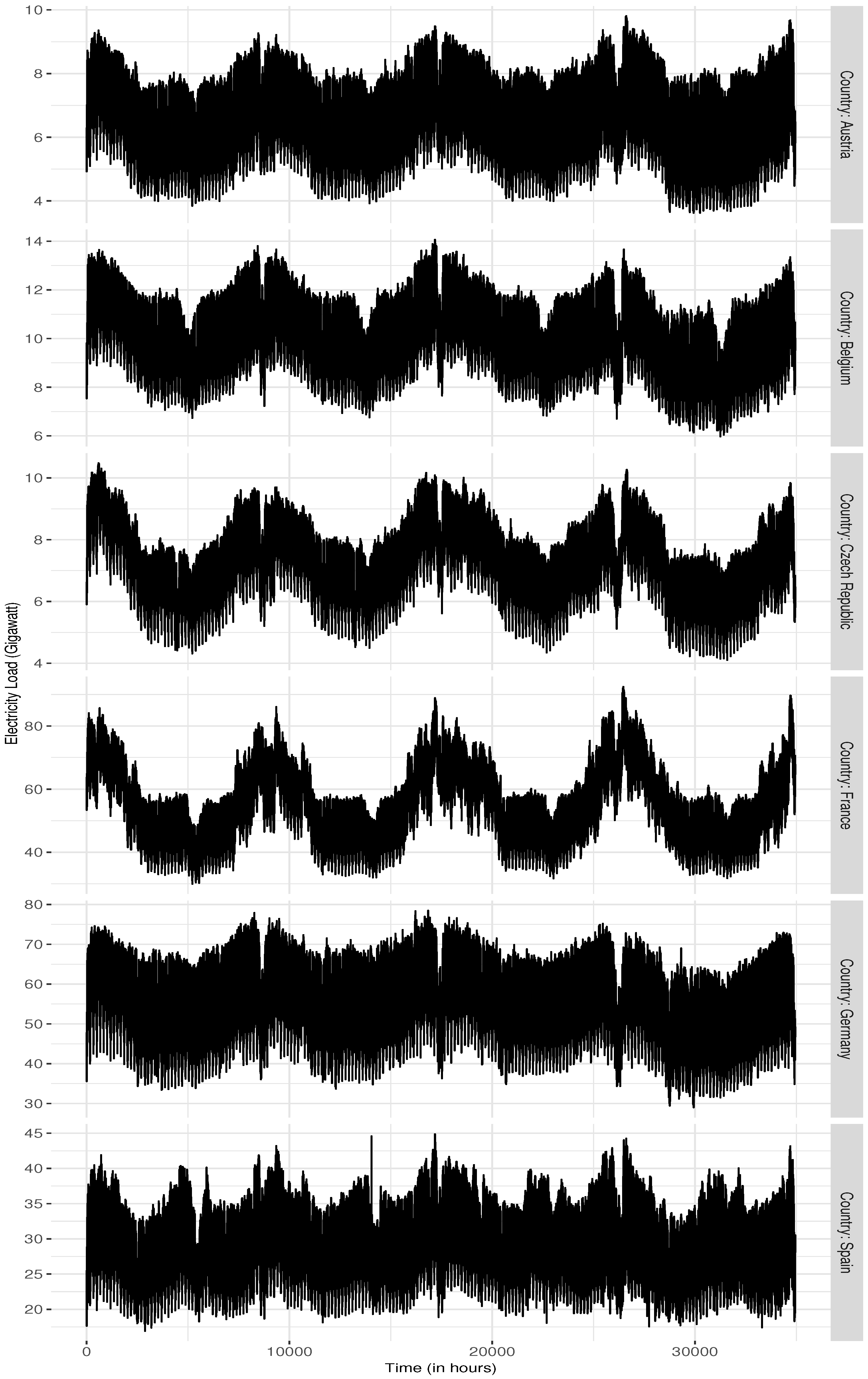
4.2. Applications on Real Hourly Electricity Load Datasets

We apply in this section the proposed Bayesian identification procedure of TSAR models to real hourly time series datasets with three layers of seasonality. These datasets are electricity load per hour collected during about four years, from Saturday 1 January 2006 to Thursday 31 December 2009, in six European countries. These electricity load datasets are characterized by exhibiting three seasonality layers: intraday, intraweek and intrayear patterns. The time plots for these time series datasets of electricity load are displayed in Figure 1. For more details about these electricity load datasets, the reader are referred to Amin [26], where these datasets are first introduced and analyzed.

Figure 1. Time plots for electricity load datasets in European countries.

It is clear from Figure 1 that the seasonality with three layers is very strong in these hourly electricity load time series; accordingly, we set the maximum order values of the TSAR model as $k_1=k_2=k_3=k_4=4$, and we apply our proposed Bayesian identification procedure for the TSAR model with the same design of the simulation study using Jeffreys’ prior and the g prior with $g=ln(q+1)/ln\left(n\right)$. We present the results of the identified TSAR model for each one of these electricity load datasets in Table 5.

Table 5. Identified TSAR models for electricity load datasets.

Time Series Dataset	Jeffreys’ Prior	g Prior ($\mathit{g}=\mathit{ln}(\mathit{q}+1)/\mathit{ln}\left(\mathit{n}\right)$)
Austria	TSAR(4)(2)${}_{24}$(4)${}_{168}$(4)${}_{8736}$	TSAR(4)(2)${}_{24}$(4)${}_{168}$(4)${}_{8736}$
Belgium	TSAR(2)(4)${}_{24}$(4)${}_{168}$(3)${}_{8736}$	TSAR(2)(4)${}_{24}$(4)${}_{168}$(3)${}_{8736}$
Czech Republic	TSAR(4)(4)${}_{24}$(4)${}_{168}$(3)${}_{8736}$	TSAR(4)(4)${}_{24}$(4)${}_{168}$(3)${}_{8736}$
France	TSAR(2)(4)${}_{24}$(3)${}_{168}$(3)${}_{8736}$	TSAR(2)(4)${}_{24}$(3)${}_{168}$(3)${}_{8736}$
Germany	TSAR(2)(4)${}_{24}$(3)${}_{168}$(4)${}_{8736}$	TSAR(2)(3)${}_{24}$(3)${}_{168}$(4)${}_{8736}$
Spain	TSAR(3)(4)${}_{24}$(4)${}_{168}$(3)${}_{8736}$	TSAR(3)(3)${}_{24}$(4)${}_{168}$(3)${}_{8736}$

We can observe from the results of this real application in Table 5 that the proposed identification procedure identifies almost the same TSAR model for the electricity load datasets that have the same stochastic behavior, as displayed in Figure 1. In addition, the identified TSAR models for these electricity load datasets are very similar for both Jeffreys’ and g priors.

5. Conclusions

In this paper, we introduced a Bayesian identification procedure for TSAR models proposed to fit and model time series with triple seasonality. We first employed three prior distributions, i.e., Jeffreys’, g and normal-gamma priors, on the TSAR model coefficients and precision, and also we assumed that the TSAR model errors are identically and normally distributed. We then derived the marginal posteriors of the TSAR model coefficients vector and precision to be the multivariate t and gamma distributions, respectively. Using the derived marginal posterior of the TSAR model coefficients, we straightforwardly proposed an identification procedure for determining the best order of TSAR models based on a sequence of t-test of significance. We conducted an extensive simulation study and the simulation results confirmed the accuracy of the proposed Bayesian TSAR identification, and also we applied our proposed procedure to real hourly electricity load datasets in six European countries. Since the current work considers only the autoregressive component, future work may include considering the moving average component in the time series model [8] and may also include an extension to the multivariate time series models [32].

References

- Taylor, J.W. Triple seasonal methods for short-term electricity demand forecasting. Eur. J. Oper. Res. 2010, 204, 139–152. [Google Scholar] [CrossRef]
- Taylor, J.W. A comparison of univariate time series methods for forecasting intraday arrivals at a call center. Manag. Sci. 2008, 54, 253–265. [Google Scholar] [CrossRef]
- Taylor, J.W. An evaluation of methods for very short-term load forecasting using minute-by-minute British data. Int. J. Forecast. 2008, 24, 645–658. [Google Scholar] [CrossRef]
- Taylor, J.W. Exponentially weighted methods for forecasting intraday time series with multiple seasonal cycles. Int. J. Forecast. 2010, 26, 627–646. [Google Scholar] [CrossRef]
- Taylor, J.W.; Snyder, R.D. Forecasting intraday time series with multiple seasonal cycles using parsimonious seasonal exponential smoothing. Omega 2012, 40, 748–757. [Google Scholar] [CrossRef]
- De Livera, A.M.; Hyndman, R.J.; Snyder, R.D. Forecasting time series with complex seasonal patterns using exponential smoothing. J. Am. Stat. Assoc. 2011, 106, 1513–1527. [Google Scholar] [CrossRef]
- Sulandari, W.; Suhartono, S.; Rodrigues, P.C. Exponential Smoothing on Modeling and Forecasting Multiple Seasonal Time Series: An Overview. Fluct. Noise Lett. 2021, 20, 2130003. [Google Scholar] [CrossRef]
- Shaarawy, S.; Broemeling, L. Bayesian inferences and forecasts with moving averages processes. Commun. Stat.-Theory Methods 1984, 13, 1871–1888. [Google Scholar] [CrossRef]
- Shaarawy, S.; Ismail, M. Bayesian inference for seasonal ARMA models. Egypt. Stat. J. 1987, 31, 323–336. [Google Scholar]
- Shaarawy, S.M.; Ali, S.S. Bayesian identification of seasonal autoregressive models. Commun. Stat.-Theory Methods 2003, 32, 1067–1084. [Google Scholar] [CrossRef]
- Barnett, G.; Kohn, R.; Sheather, S. Robust Bayesian Estimation Of Autoregressive–Moving-Average Models. J. Time Ser. Anal. 1997, 18, 11–28. [Google Scholar] [CrossRef]
- Vermaak, J.; Niranjan, M.; Godsill, S.J. Markov Chain Monte Carlo Estimation for the Seasonal Autoregressive Process with Application to Pitch Modelling; Technical Report; Department of Engineering, University of Cambridge: Cambridge, UK, 1998. [Google Scholar]
- Amin, A.A. Bayesian Inference of Triple Seasonal Autoregressive Models. Pak. J. Stat. Oper. Res. 2022, 18, 853–865. [Google Scholar] [CrossRef]
- Amin, A.A.; Emam, W.; Tashkandy, Y.; Chesneau, C. Bayesian Subset Selection of Seasonal Autoregressive Models. Mathematics 2023, 11, 2878. [Google Scholar] [CrossRef]
- Barnett, G.; Kohn, R.; Sheather, S. Bayesian estimation of an autoregressive model using Markov chain Monte Carlo. J. Econom. 1996, 74, 237–254. [Google Scholar] [CrossRef]
- Ismail, M.A. Bayesian Analysis of Seasonal Autoregressive Models. J. Appl. Stat. Sci. 2003, 12, 123–136. [Google Scholar]
- Ismail, M.A. Bayesian Analysis of the Seasonal Moving Average Model: A Gibbs Sampling Approach. Jpn. J. Appl. Stat. 2003, 32, 61–75. [Google Scholar] [CrossRef]
- Ismail, M.A.; Amin, A.A. Gibbs sampling for SARMA models. Pak. J. Stat. 2014, 30, 153–168. [Google Scholar]
- Amin, A. Gibbs Sampling for Bayesian Prediction of SARMA Processes. Pak. J. Stat. Oper. Res. 2019, 15, 397–418. [Google Scholar] [CrossRef]
- Ismail, M.A.; Zahran, A.R. Bayesian inference on double seasonal autoregressive models. J. Appl. Stat. Sci. 2013, 21, 13. [Google Scholar]
- Amin, A. Gibbs sampling for double seasonal ARMA models. In Proceedings of the 29th Annual International Conference on Statistics and Computer Modeling in Human and Social Sciences, Cairo, Egypt, 28–30 March 2017. [Google Scholar]
- Amin, A.A. Bayesian inference for double SARMA models. Commun. Stat.-Theory Methods 2018, 47, 5333–5345. [Google Scholar] [CrossRef]
- Amin, A.A. Bayesian identification of double seasonal autoregressive time series models. Commun. Stat.-Simul. Comput. 2019, 48, 2501–2511. [Google Scholar] [CrossRef]
- Amin, A.A. Bayesian analysis of double seasonal autoregressive models. Sankhya B 2020, 82, 328–352. [Google Scholar] [CrossRef]
- Amin, A.A. Full Bayesian analysis of double seasonal autoregressive models with real applications. J. Appl. Stat. 2023, 1–21. [Google Scholar] [CrossRef]
- Amin, A.A. Gibbs sampling for Bayesian estimation of triple seasonal autoregressive models. Commun. Stat.-Theory Methods 2023, 52, 7303–7322. [Google Scholar] [CrossRef]
- Broemeling, L.D. Bayesian Analysis of Linear Models; CRC Press: Boca Raton, FL, USA, 1985. [Google Scholar]
- Broemeling, L.D. Bayesian Analysis of Time Series; CRC Press: Boca Raton, FL, USA, 2019. [Google Scholar]
- Fernandez, C.; Ley, E.; Steel, M.F. Benchmark priors for Bayesian model averaging. J. Econom. 2001, 100, 381–427. [Google Scholar] [CrossRef]
- Box, G.E.; Tiao, G. Bayesian Inference in Statistical Analysis; John Wiley & Sons: Hoboken, NJ, USA, 1973. [Google Scholar]
- Lütkepohl, H. New Introduction to Multiple Time Series Analysis; Springer Science & Business Media: Berlin/Heidelberg, Germany, 2005. [Google Scholar]
- Reinsel, G.C. Elements of Multivariate Time Series Analysis; Springer Science & Business Media: Berlin/Heidelberg, Germany, 2003. [Google Scholar]
Disclaimer/Publisher’s Note: The statements, opinions and data contained in all publications are solely those of the individual author(s) and contributor(s) and not of MDPI and/or the editor(s). MDPI and/or the editor(s) disclaim responsibility for any injury to people or property resulting from any ideas, methods, instructions or products referred to in the content. |
© 2023 by the authors. Licensee MDPI, Basel, Switzerland. This article is an open access article distributed under the terms and conditions of the Creative Commons Attribution (CC BY) license (https://creativecommons.org/licenses/by/4.0/).