A Variable Neighborhood Search Method with a Tabu List and Local Search for Optimizing Routing in Trucks in Maritime Ports

Abstract

Logistics problems represent an important class of real-world problems where even small improvements in solution quality can lead to significant decreases in operational costs. However, these problems are usually NP-hard; thus, they are mostly solved using metaheuristic methods. To improve their performance, there is substantial research on crafting new and refined metaheuristics to derive superior solutions. This paper considers a truck routing problem within a naval port, where the objective is to minimize the total distance traveled by all the vehicles to distribute a given set of containers. Due to the large volume of goods that are being transferred through ports, it is imperative to improve the operation times at such ports to improve the throughput. To achieve this goal, a novel variable neighborhood search method that integrates a tabu list, an iterative local search procedure, and parallelization of neighborhood generation is proposed and evaluated. The experimental results demonstrate that the proposed method achieves similar results to the state of the art, but in a smaller amount of time.

1. Introduction

The vehicle routing problem is an interesting and well-studied research topic due to its growing impact on real-world industrial processes [1]. Well-planned vehicle routes can significantly reduce overall costs and resource requirements in the transportation sector. Simple optimization objectives, such as minimizing transportation distances or reducing fuel consumption by taking faster routes, can make a significant difference and result in highly efficient systems. However, since these objectives are often not sufficient, more advanced methods incorporate additional constraints. Some of these include balancing the workload among vehicles [2], coordinating adjacent shifts [3], avoiding traffic congestion [4], and dynamically updating vehicle routes [5]. The optimization objectives depend on the specific problem and customer requirements, and there are numerous different objectives that often need to be balanced [6]. Furthermore, in such problems, we are often faced with different kinds of uncertainties that also need to be taken into account, and develop approaches that can work with them need to be developed [7]. In addition to substantial financial benefits, effective route and shift planning can improve driver safety and job satisfaction, reducing the number of vehicles and minimizing the environmental impact. Therefore, companies whose business operations involve the transportation of goods have great interest in this topic to leverage the benefits of optimization.

A concrete example is the Ningbo port on the coast of the East China Sea, which holds the status of the world’s largest port in terms of cargo throughput. In 2021, the port handled 1.224 billion tons of cargo (https://www.nbport.com.cn/gfww/, accessed on 13 July 2023). This figure represents a significant logistical challenge as such a large volume of cargo requires excellent organization and transportation planning. In addition to route planning, it is necessary to coordinate all related processes, such as vehicle preparation and maintenance, traffic updates, and vehicle location monitoring. At the same time, there is a great opportunity for cost savings as even small improvements in the system can lead to significant cost reductions overall. In such cases, it is crucial to minimize the resources consumed in transporting goods.

All of the above calls for the development of a system aimed at optimizing vehicle routing. The described problem is a well-known vehicle routing problem (VRP) that has been studied for over 60 years since it was first mentioned by Dantzig and Ramser [8]. Over the years, VRP has been successfully integrated with other technologies to develop so-called “smart cities” and “smart ports” (https://commission.europa.eu/eu-regional-and-urban-development/topics/cities-and-urban-development/city-initiatives/smart-cities_en, 13 July 2023). The idea behind such projects is to develop highly efficient systems that seek to optimize, among other things, the transportation of people and goods to increase the satisfaction and safety of citizens or employees. These systems utilize various technologies to collect as much data as possible, including GPS, radar and sensor technology, 5G networks, and Internet of Things (IoT)-connected technologies. Subsequently, through the analysis of big data, these data are transformed into valuable information used to assess transportation needs. A good vehicle routing algorithm forms the core of such a system and is essential for a successful end product. In this regard, there are different variants of VRP, depending on the specific constraints that the algorithm must consider, such as time windows (VRPTWs) [9], time-dependent travel duration (TDVRP) [10], pickup and deliveries (VRPPDs) [11], fleets with electric vehicles [12,13], and many others [14,15,16].

In the particular case of the Ningbo port, we are dealing with the open periodic vehicle routing problem with time windows (OPVRPTWs). The network of each maritime port consists of several surrounding nodes (cities) between which container transportation is required. This transportation from the origin location to the destination is constructed as a single task that has a start and end time within which the goods need to be transported (thus, the problem includes time windows). Furthermore, since the transportation tasks are specified across several periods (shifts) and in some shifts the vehicle does not need to return to the depot, it is an open and periodic problem. These additional properties introduce additional constraints that need to be considered when constructing a solution.

In order to deal with the previously described problem, we propose a novel variable neighborhood search (VNS) algorithm that uses several neighborhood structures from the literature and applies them in several layers during the execution, depending on whether the algorithm is focused on exploitation or exploration. Additionally, we introduce a tabu list into the algorithm to help the algorithm avoid areas of the search space that it already visited. Furthermore, to gain additional performance improvements, the neighborhood search is parallelized. We denote the resulting algorithm as VNTS and evaluate its performance on a set of real-world and artificially generated instances for OPVRPTWs based on the real-world logistics problem from the Ningbo port. Certain algorithm design choices are evaluated and the algorithm is compared to the state-of-the-art results from the literature. The experimental study demonstrates that the proposed algorithm achieves slightly better results than an existing algorithm from the literature, but in a significantly smaller amount of time.

The rest of the paper is organized as follows. The next section provides a short overview of the literature dealing with VRS, specifically with OPVRPTWs. Section 3 provides the description of the problem under consideration. Section 4 describes the proposed method used to solve the routing problem. The experimental setup is described in Section 5, whereas the results of the executed experiments are summarized in Section 6. Finally, Section 7 concludes the paper and outlines possible future research directions.

2. Literature Review

VRP is of great interest due to the significant advantages it offers through the implementation of an effective system. The opportunity for resource savings attracts many researchers and industry leaders to explore and improve existing methods. This leads to a large number of research studies in this field, each taking different approaches due to the various variants of the problem and the different optimization objectives and constraints involved [6,17]. Since finding the optimal solution for the most challenging instances of this problem is extremely difficult (if not impossible) within a reasonable time frame, the challenge lies in evaluating what constitutes “good” solutions. However, the term “good” can have subjective meanings, especially in this context. Therefore, it is important to compare different approaches and understand the strengths and weaknesses of each. There is no universal approach that can solve all such problems in the best possible way (as stated in the “No Free Lunch” theorem).

The nature of the problem itself excludes an exact approach due to the large search space. Even in small instances, existing deterministic methods cannot provide high-quality solutions within a reasonable time [18]. Each day requires the transportation of hundreds of containers, with their time windows spanning across several possible shifts [19]. An exact, deterministic approach is only feasible for smaller problems or comparison purposes when time is not a crucial factor [20,21]. The reality is that such cases are in the minority, making it necessary to find more advanced approaches capable of solving real-world complex problems.

Therefore, evolutionary approaches have received significant attention throughout history as they can relatively successfully find “good enough” solutions within a reasonable time frame. However, these approaches also have limitations, particularly for very large instances, but their inefficiency is often highlighted as a significant drawback [22]. Poorly implemented evolutionary algorithms can be highly inefficient if the search is not directed effectively, resulting in suboptimal solutions, despite having ample time available. If time is critical in problem-solving, we need an approach that can search the space of possible solutions relatively quickly and efficiently.

It has been shown that population-based approaches are not the most efficient for solving problems with a large search space since adding complexity (the number of solutions in one generation) to the system significantly slows down the algorithm [18]. On the other hand, if time is not a crucial factor, slower but ultimately better solutions are more interesting. In this regard, population-based approaches can still be a good option depending on the complexity of the problem and the implementation. For example, refs [23,24] successfully implement genetic algorithms for solving simpler problems, while the authors of [25,26] implement ant colony algorithms for solving VRP. These algorithms are relatively effective in this context as they address smaller-scale problems that are less common in today’s world.

As for the initialization of the initial solution, there is a well-known technique called “insertion” that was introduced by Clarke and Wright [27]. Over the years, other initialization techniques have been developed that are faster and simpler. It has been shown that a good initial solution does not necessarily result in a better final solution, so researchers often opt for the simplest and fastest initialization option to reduce the algorithm’s complexity [18]. Efficiently initializing a good solution is, therefore, the foundation of a good system that can quickly find a “good enough” solution for the given problem. In addition, complexity is of utmost importance because there is constantly updated real-time information about the location of vehicles, and these systems often have graphical interfaces through which vehicles and routes are observed, requiring fast execution. Additionally, there may be a need to gradually update routes based on various situations, such as traffic congestion, road works, obstacles, etc. In [28], the authors discuss the impact of complex constraints on the complexity of initialization for the general VRP case and propose an efficient insertion heuristic with a complexity of $O\left(n^3\right)$ and, in some rare cases, $O\left(n^{3}logn\right)$. This is a significant improvement compared to the usual approach with a complexity of $O\left(n^4\right)$. Reducing complexity offers exactly what was described earlier: efficient initialization and the possibility of iterative improvement using an evolutionary approach and/or local search if necessary.

Because of the previous reasons, recent research has dominantly applied various kinds of local search and variable neighborhood methods to solve various VRPs [18,29,30]. This is also the case with the OPVRPTW problem considered in this paper. The problem of routing trucks in a maritime port based on the example of the Ningbo port was first considered in [19]. The authors provide a formal definition of the newly proposed problem and also design a two-stage algorithm in order to solve the proposed problem. In the first stage, a simple initial solution method is used to construct the initial solution, which is then improved with a VNS algorithm in the second phase. The results demonstrate that the proposed algorithm achieved a performance improvement of 5–10% when compared to the results in practice, thus demonstrating the benefit of applying such approaches.

Within the scope of [31], the neighborhood is examined, and path weights are updated as a measure of goodness to find better solutions to the traveling salesman problem in combination with a genetic algorithm. The neighborhood refers to solutions that can be obtained by making certain changes to the current solution. In the context of vehicle routing, these changes often involve destroying a certain number of routes and inserting the corresponding tasks at different locations within the solution. Additionally, smaller changes are possible, such as altering the order of tasks within a route or changing the location of a task to a different route. In [32], an adaptive variable neighborhood search technique is used, and a set of solution destruction and repair operators that have proven successful are proposed to create the neighborhood. The obtained results demonstrate that the proposed algorithm can further improve the best solutions obtained for the problem. A bi-objective variant of the problem is investigated in [33], in which the total travel distance and driver payment criteria are minimized. The authors propose the application of a hyper-heuristic approach to solve this problem variant, in which five heuristics with different levels of perturbations are used. The results outline that the algorithm is able to obtain Pareto fronts of good final quality, better than other state-of-the-art algorithms when tested on this problem. In [18], a common variable neighborhood search technique is employed along with a more advanced search routing system. The algorithm examines neighboring states (solutions) and updates certain parameters based on them to guide further searches. If the neighboring states are promising, it indicates that the current solution is in a high-quality search space and that the algorithm continues searching in the same direction. However, if the neighboring states around the current one are of low quality, the search direction is changed to explore a sub-space of better quality. This approach has shown promise, although the large number of parameters requires careful tuning.

The existence of a large number of completely different algorithms that can relatively successfully solve variants of similar problems further confirms that there is no universal approach that efficiently solves all of these problems. However, numerous research studies and advancements in the field have led to more robust approaches that, through data analysis (e.g., the network for distributing goods, frequency of container transfers on specific routes, weather forecasts, road conditions, etc.), can gain valuable insights into the problem and adapt the approach and specific parameters to better fit the given problem. This increases the efficiency of the algorithm and ultimately leads to better final solutions.

3. Open Periodic Vehicle Routing Problem with Time Windows

3.1. Problem Description

The problem under consideration can be classified as an open periodic vehicle routing problem with time windows (OPVRPTWs) that is modeled based on a practical problem from the real world encountered at the Ningbo port, one of the largest ports in China [19].

In the considered problem, a certain number of containers needs to be transported between cities within the network. Each container i has a time window $[a_i,b_i]$ associated with it, which defines the earliest time from which the container can be picked up from the source destination ($a_i$) and the latest that the container has to be delivered to the destination ($b_i$). The vehicle fleet owned by Ningbo port consists of 100 identical vehicles [19] that can transport only one container at a time. Adhering to local labor laws, shifts for task execution are divided into two shift types, day and night shifts, each lasting 12 h. Therefore, the first shift of the day starts at 08:00 a.m., and the second shift starts at 08:00 p.m. The shifts are indexed in chronological order, with odd indices representing day shifts and even indices representing night shifts. The analysis of task deadlines has shown that the majority of these deadlines fall within day shifts. However, most tasks have a wide range of possible shifts, so it is possible to distribute tasks equally between day and night shifts. During these shifts, drivers carry out tasks by transporting containers from one city to another. It is important to note that vehicles do not return to the central warehouse at the end of the day shift; they only do so at the end of the night shift. Therefore, the idea when creating the route for the day shift is to construct a path that takes into account the next shift and ends at the node (city) where the next shift begins, thus making these two shift types a kind of unity. This reduces the proportion of so-called empty trips, during which vehicles do not carry cargo but only travel to the location that represents the source of the next task. Such parts of the route represent a significant cost since no work is performed within them; the driver only prepares the vehicle for the next task.

Since the total distance of cargo transportation is fixed (determined by the predefined tasks), the main goal of the problem is to minimize the proportion of empty trips. This is used as an indicator of solution quality and can be abbreviated as the LDR (loaded distance rate), which is a commonly used measure in the logistics sector. If the cargo transportation distance is expressed by the measured LD (loaded distance) and the distance of empty trips is expressed by the measured UD (unloaded distance), LDR can be calculated as follows:

$$LDR=\frac{LD}{LD+UD}.$$

Since this metric measures the proportion of the distance traveled with the load in the total traveled distance, it needs to be maximized. When presenting the results and comparing different methods, the LDR metric will be used to assess the quality of the results.

Therefore, individual tasks have time windows within which they must be completed, and vehicles must return to the warehouse at the end of every second shift. This means that this is an open problem of vehicle routing with time windows (OPVRPTWs). The described problem differs from the classical VRP because goods are transported between all nodes, not just from a central warehouse to other nodes. The problem has elements of pickup and delivery vehicle routing (VRP with PD), but it differs in that the vehicle’s capacity is only one container, and the vehicle can perform only one job at a time. (The vehicle never transports goods to two different destinations at the same time.) The analysis of specific problem instances has shown that the frequency of routes between all nodes is equal, which means that all nodes are equally important (except for vehicle storage, where the central warehouse is the only option). However, special attention should be paid to the node that connects the day shift with the night shift. As mentioned, in the ideal situation, the destination of the last task of the day shift is the same as the source of the first task of the night shift. This outcome is desirable because the shift change does not involve an empty trip, but it may not always be possible to achieve. In cases where such vehicle routing is not possible, the following approach is taken. If the driver of the day shift has time during their working hours to prepare the vehicle for the first task of the night shift, they will drive an empty vehicle from the destination of their last task to that node. If the driver cannot do this before the end of their working hours, they will leave the vehicle at the destination of their last completed task. The driver of the night shift will then have to perform an empty trip as the first part of their route to reach the source of their first task.

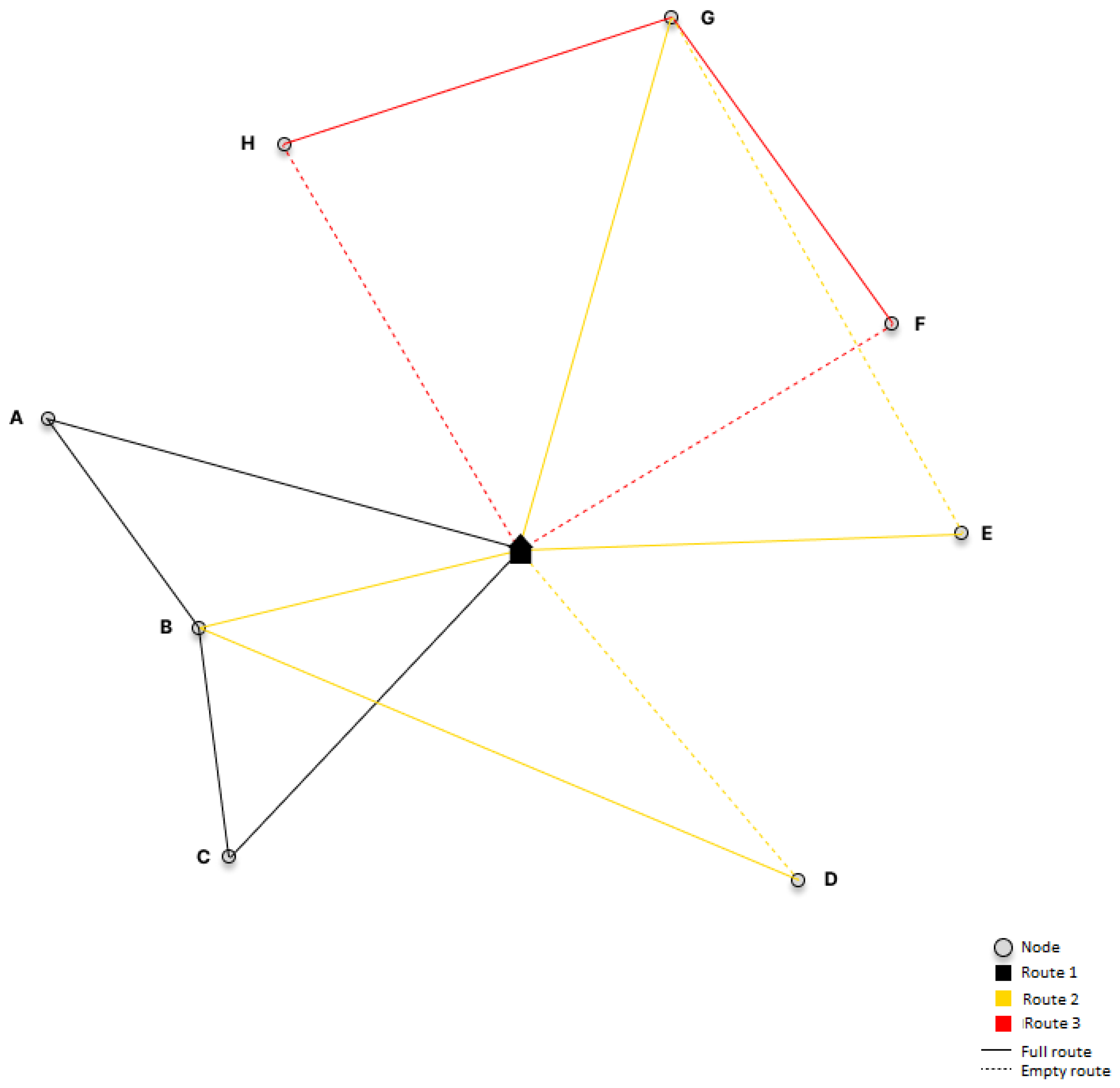
Figure 1 shows an example of created routes for three vehicles in two shifts. Each color represents a route performed by one vehicle. At the beginning of the day shift, the vehicle starts from the warehouse (located at the center) and performs tasks. When it is time for the shift change, the vehicle is taken over by the driver responsible for the night shift and continues with the tasks. At the end of their shift, the driver must return the vehicle to the warehouse. Let us consider the quality of each route. If we know that solid lines represent parts of routes where tasks are performed, and dashed lines represent empty trips during which vehicles do not perform any work, it is evident that the black route is the most efficient as it has no empty trips. On the other hand, the red route is not of good quality as it has a significant proportion of empty trips. Furthermore, as we can see, each node can be visited several times by vehicles, which is determined by the number of tasks that have that node as a source or destination.

Figure 1. Example of several vehicle routes.

Because vehicles return to the warehouse at the end of every second shift, the algorithm searches for routes rather than cycles, as in the case of the classical VRP. However, this problem is not the same as the school bus routing problem, where the day and night routes are identical. In fact, the two routes of a single vehicle belonging to the day shift and the next night shift do not have to be identical and usually will not be. Furthermore, in many VRP cases, the loading and unloading times of goods can be ignored since they are relatively short compared to the transportation time of goods. However, here it is not the case. The loading and unloading times of goods are significant and must be taken into account in the time calculations. The cities are relatively close, and the transportation time of goods is not significantly longer than the loading and unloading times.

3.2. Problem Definition

Table 1 presents the notations used to define the mathematical model, which was defined in [18,33]. The purpose of this definition is to clearly indicate all constraints and the optimization objective.

Table 1. List of symbols used for the definition of the mathematical model of the problem.

Symbol	Description
K	Total number of vehicles available in each shift
N	Number of nodes (cities) between which the goods are transported
D	Set of days sorted by date
S	Set of shifts sorted by date
$[S_s,S_e]$	Time window of the shift S
$S_{day}$	Set of day shifts sorted by date, indexed by odd numbers
$S_{night}$	Set of night shifts sorted by date and indexed by even numbers
T	The set of tasks that have to be completed
$[a_i,b_i]$	The time window of task i. The task has to start executing within the given time window.
$l_i$	Time required to complete the task i
$T_i$	The time moment of reaching the source node of the task i
$B_i$	The time moment of starting to execute task i
$t_{ij}$	The travel time (in minutes) from node i to node j
$d_{ij}$	The travel distance of the trip from node i to node j
$x_{ij}^s$	Binary decision variable that denotes whether the task with the source in i and destination in j was completed in the shift s

The number of vehicles K represents the size of a homogeneous fleet of vehicles available in each shift. Each individual vehicle can transport a maximum of one container at a time. Containers are transported between nodes N, and for each node, the loading and unloading times for one container are known. The days within the horizon of a specific instance are denoted as D and indexed sequentially starting from one. Each day has a day shift ($S_{day}$) and/or a night shift ($S_{night}$), depending on the exact horizon boundary, i.e., whether the respective shift falls within the horizon where tasks T need to be performed. However, the boundary days may not have both shifts if they do not belong to the horizon where tasks need to be performed. Each shift has its start and end time, which is equal to the start and end time of the driver’s work shift assigned to that shift. Each task has a source and destination city and the earliest possible start time $a_i$ and latest time $b_i$ for starting the task.

It is important to note that if a vehicle arrives at the task’s source node before its time window, it must wait until $a_i$. Tasks that involve multiple containers are divided into multiple smaller tasks so that each individual task only requires the transportation of one container. This simplification facilitates the problem formulation and improves the efficiency of the proposed algorithm by making task allocation easier. Furthermore, the task execution time $l_i$ includes loading at the source, transportation to the destination, and unloading at the destination. The travel time and distance between two nodes are represented by $t_{ij}$ and $d_{ij}$, respectively. For the purpose of defining constraints, the start time of task i is denoted by $B_i$. The travel time is expressed in minutes, which is important for calculating the feasibility of solutions, while travel distances are expressed in kilometers. However, the unit of distance can be ignored because the evaluation of the solution quality is based on the proportion of the transportation distance to the total sum of vehicle routes (transportation and empty trips). Finally, the binary decision variable $x_{ij}^s$ indicates whether a specific task with origin i and destination j is performed in shift s. These notations are also used in [18], with minor modifications.

Using the notation introduced above, we can now define the mathematical optimization problem that needs to be solved:

$$\begin{array}{c}minimizeF\left(x\right)=\sum _{s\in S}\sum _{i\in T}\sum _{j\in T}{d}_{ij}·x_{ij}^s\end{array}$$

(1)

subject to:

$$\begin{array}{c}\hfill \sum _{s\in S}\sum _{i\in T}{x}_{ij}^s=1,\forall j\in T\end{array}$$

(2)

$$\begin{array}{c}\hfill \sum _{s\in S}\sum _{j\in T}{x}_{ij}^s=1,\forall i\in T\end{array}$$

(3)

$$\begin{array}{c}\hfill a_i\le B_i\le b_i-l_i\forall i\in T\end{array}$$

(4)

$$\begin{array}{c}\hfill x_{ij}^s\ast S_s\le x_{ij}^s\ast T_i\forall i\in T,\forall j\in T,\forall s\in S\end{array}$$

(5)

$$\begin{array}{c}\hfill x_{ij}^s\ast (B_i+l_i)\le x_{ij}^s\ast E_s\forall i\in T,\forall j\in T,\forall s\in S\end{array}$$

(6)

$$\begin{array}{c}\hfill x_{ij}^s\in \{0,1\}\forall i\in T,\forall j\in T,\forall s\in S\end{array}$$

(7)

$$\begin{array}{c}\hfill \sum _{j\in N}{x}_{0j}^s=K,\forall s\in S_{day}\end{array}$$

(8)

$$\begin{array}{c}\hfill \sum _{i\in N}{x}_{i0}^s=K,\forall s\in S_{night}\end{array}$$

(9)

The objective function denoted as 1 signifies that the goal is to minimize the total route distance of all vehicles. Since the distance of cargo transportation is fixed and determined by the specific tasks that constitute the instance, the objective is to minimize the proportion of empty trips, in other words, to maximize the LDR while respecting all given constraints. Constraints 2 and 3 indicate that each task is performed exactly once and that all tasks are completed. Constraint 4 ensures that work on each task starts within its time window. Constraints 5 and 6 specify that the work of a single vehicle is performed within the time window of one shift. This is done by using $x_{ij}^s$ to filter the corresponding starting or ending time of the shift to which the task is associated, and checking whether the starting and completion times of the task are within them. Constraint 7 states that the decision variable is binary, meaning it can only take values of one or zero. Again, in this OVRP, vehicles return to the warehouse at the end of every second shift. This is ensured by defining constraints 8 (for the day shift) and 9 (for the night shift). Additionally, these constraints ensure compliance with the constraints on the maximum number of vehicles in a shift.

The conclusion from the analysis and formal problem definition is that this is a nonlinear constrained problem with a vast search space. The size of the search space is determined by the length of the horizon $\left(\right|\mathit{S}\left|\right)$, the number of vehicles $\left(\mathit{K}\right)$, and the number of tasks $\left(\right|\mathit{T}\left|\right)$. Since the total number of possible routes in the solution is equal to $\left|S\right|\ast K$, and the number of task permutations is $\left|T\right|!$, the size of the search space is $\left|S\right|\ast K\ast \left|T\right|!$ [18]. Therefore, it is logical to conclude that a high-quality algorithm is necessary to find a relatively good solution by effectively navigating the search space.

4. Variable Neighborhood Search with Tabu List and Iterated Local Search

To solve the previously outlined OPVRPTW problem, we propose a novel variable neighborhood search (VNS) method that includes a tabu list and iterates a local search procedure, denoted as the variable neighborhood tabu search (VNTS). The parameters that control the behaviors of the algorithm are outlined in Table 2. Some parameters are adaptable and change during the execution of the algorithm so that it can better adapt to the current conditions of the search. The parameters that change during the execution of the algorithm are the route and task multipliers, which control how much of the solution will be destroyed to construct a new solution, as well as the number of neighborhood layers and neighbors generated in each layer, the values of which must be within the interval specified by the user. The remaining parameters are fixed through the entire execution of the algorithm.

Table 2. Overview of the algorithm parameters.

Name	Description
Fixed-value parameters
Diversification period (DP)	Defines the number of iterations between two subsequent diversification periods
Incumbent improvement (IM)	Defines the number of iterations to wait for improvement before switching to diversification
Local search iterations (LSI)	The number of iterations that the local search procedure performs
Minimum number of layers (MinL)	The minimum allowed number of layers that are used to create the neighboring solutions
Maximum number of layers (MaxL)	The maximum allowed number of layers that are used to create the neighboring solutions
Minimum number of neighbors (MinN)	The minimum allowed number of neighbors created in a layer
Maximum number of neighbors (MaxN)	The maximum allowed number of neighbors created in a layer
Neighbor multiplier (NM)	Number of neighbors that should be generated in each layer
Tabu list size (TLS)	Size of the tabu list that keeps track of recently visited solutions
Adaptive parameters
Route multiplier (RM)	Multiplier used to determine the number of routes that will be removed in each neighborhood layer
Task multiplier (TM)	Multiplier used to determine the number of tasks that will be removed in each neighborhood layer

The general outline of the VNTS algorithm is given in Algorithm 1. At the start of the algorithm, the previously outlined parameters have to be set by the user. After that, and depending on the problem instance that is solved, an initial solution is constructed using a certain heuristic procedure. Selected potential procedures to construct the initial solution are described in Section 4.1. After the parameter and solution initialization process, the main loop of the algorithm is executed until a given termination criterion is reached, which in this case will be the amount of the elapsed time.

In the main loop of the algorithm, the first operation is the adaptation of certain algorithm parameters, depending on the recent history of the search, in order to facilitate either intensification or diversification. The update process of the parameters is outlined in Section 4.2. After the algorithm parameters have been updated, a neighborhood search is performed through several layers that control the intensity of operators that are used to perturb the solution. Depending on the current value of respective parameters, the algorithm will perform a broad or restricted search in the neighborhood of the current solution. Both the number of neighbors and the extent to which the current solution will be perturbed depend on the current neighborhood layer and the appropriate multiplier parameters. The number of neighbors (NN) that will be constructed in a certain layer is calculated as

$$NN=min(MinN+2\ast i,MaxN),$$

where i denotes the index of the current layer. Furthermore, the route and task numbers that are removed from the current solution when generating neighbors are

$$TtR=TM\ast i,$$

$$RtR=RM\ast i,$$

where $TtR$ denotes the number of tasks that will be removed from the solution, $RtR$ denotes the number of routes that will be removed, and i denotes the index of the current neighborhood layer. In this way, each subsequent layer not only generates more neighbors, it also generates more distinct neighbors as it will introduce larger perturbations in the current solution. Based on these parameters, the neighborhood of the current solution is generated as explained in Section 4.3.

Out of the generated neighborhood, the best solution that is not in the tabu list is selected. This solution is then set as the current solution since it was found to be better to accept every new solution rather than accepting only better solutions. In this way, the algorithm has more of a chance to escape the local optima and the algorithm introduces more diversity in its search process. In the final step, an additional local search procedure, described in Section 4.4, is applied to the current solution to further intensify the search. The complexity of one iteration of the algorithm in the notion of generated neighbors is equal to $L\times N$, where L is the number of layers and N represents the number of neighbors generated in each iteration. However, as the number of layers and neighbors is adaptable during the algorithm execution, this can affect the amount of the computation performed in the individual iterations and is not constant during the entire execution of the algorithm.

Algorithm 1 VNTS algorithm outline
1: $P\leftarrow initialise\_parameters\left(instance\right)$	▹ Parameter initialization
2: $S\leftarrow initialise\_starting\_solution(instance,P)$	▹ Initialise starting solution
3: $iter\leftarrow 0$	▹ Iteration counter
4: $last\_improve$	▹ Iteration of last improvement
5: while $!termination\_criterion$  do
6:      $P\leftarrow adjust\_parameters(P,iter)$	▹ Adjust current parameter values
7:      while $i\le number\_of\_layers$ do
8:          $i\leftarrow i+1$
9:          $P.NN\leftarrow min(P.MinN+2\times i,P.MaxN)$	▹ Number of neighbors to generate
10:        $P.TtR\leftarrow P.TM\ast i$	▹ Number of tasks to remove
11:        $P.RtR\leftarrow P.RM\ast i$	▹ Number of routes to remove
12:        $neighborhood\leftarrow generate\_neighborhood(S,P)$
13:        for $solution\in neighborhood$ do	▹ Find the best neighbor not in the tabu list
14:              if $LDR\left(solution\right)>LDR\left(best\right)$ && !$tabu\_list.contains\left(N\right)$ then
15:                   $selected\_neighbour\leftarrow solution$
16:              end if
17:          end for
18:          if $LDR\left(S\right)<LDR\left(neighbour\right)$ then	▹ Determine if solution improved or not
19:              $last\_improve\leftarrow iter$
20:          end if
21:          $S\leftarrow neighbour$	▹ Accept the neighbor and add it to the tabu list
22:          $tabu\_list.insert\left(solution\right)$
23:      end while
24:      $S\leftarrow local\_search(S,P)$	▹ Perform additional local search for intensification
25: end while
26: return Best found solution

4.1. Solution Initialization

The initialization of the initial feasible solution is the first step of the algorithm. Several initialization types are well-known in this field. However, it has been shown that this aspect of the algorithm is not necessarily crucial because a better initial solution does not necessarily lead to a better final solution, so the fastest or simplest method of initialization is usually chosen. However, as mentioned, the complexity of the approach and the quality of the quickly generated solution are important aspects of today’s systems, so numerous initialization methods have been tested. First, the Clarke–Wright initialization method was tested, which assigns one route to each vehicle and then attempts to reduce the number of routes by merging existing routes in a way that maximally improves routing (greedy approach). This approach is well-known and frequently used in the literature. This paper will not examine it in more detail because it has been found to be slower than other methods and the obtained solution tends to get stuck in a local optimum.

A new type of initialization is proposed that creates cycles instead of routes. The method considers each daily and the following nightly shift as a whole and creates a route for that unit. This approach still respects all daily constraints (it is trivial to divide such a route into a daily and nightly shift), but it significantly simplifies the implementation and the search space exploration. Additionally, this approach implicitly aims to minimize the proportion of empty paths between the mentioned two shift types, which further enhances the quality of the solution. Furthermore, it is required to define in which order the tasks are selected in the initialization process. Here, we use three heuristic rules:

• Urgency-based insertion heuristic (UBIH)—The initialization that first assigns tasks with the earliest deadlines.
• Width-based insertion heuristic (WBIH)—The initialization method that first assigns tasks with the narrowest time windows.
• Random shuffle insertion heuristic (RSIH)—The initialization that assigns tasks in random order.

During the insertion of each task, it deliberately does not place the task in the optimal position to avoid becoming stuck in the local optimum. All mentioned initialization methods result in feasible solutions. Although it is possible to generate higher-quality initial solutions, it was not done so because it was found that good initial solutions do not necessarily lead to better final solutions. Moreover, high-quality initial solutions can quickly become trapped in a local optimum. Therefore, the priority is the speed of initialization while respecting the constraints.

4.2. Parameter Update

In each iteration of the algorithm, some parameters are updated based on the state of the search. The procedure by which the parameters are updated is outlined in Algorithm 2. In the case that the number of iterations without improvement is larger than the threshold specified by the incumbent improvement parameter (IM), the algorithm is likely stuck in the local optima, i.e., stagnation is detected. Therefore, the parameters are adjusted in a way to facilitate diversification, i.e., to explore the search for a wider region of solutions. First of all, the number of neighborhood layers is incremented if it is still lower than the allowed maximum value. Furthermore, the multipliers for task and route removal are also incremented, which will mean that a larger portion of the current solution is destroyed, thus facilitating more diversification in the newly created neighbors. However, this is done only if a certain number of iterations has elapsed since the last diversification, which is controlled by the diversification period (DP) parameter.

Algorithm 2 Parameter update procedure
1: Input:parameters P, current iteration iter, iteration of last improvement last_improve
2: if $iter-last\_improve>P.IM$ && $iter-P.last\_diversification>P.DP$ then	▹ If stagnation was detect
3:       $P.NL\leftarrow max(P.NL+1,P.MaxL)$
4:       $P.RM\leftarrow P.RM+1$
5:       $P.TM\leftarrow P.TM+1$
6:       $P.diversification\leftarrow true$
7:       $P.last\_diversification\leftarrow iter$	▹ Store when the last diversification happened
8: else if $noImprov=0$ then	▹ If improvement was detected
9:       $P.NL\leftarrow min(P.NL-1,P.MinL)$
10:     $P.RM\leftarrow 1$
11:     $P.TM\leftarrow 1$
12:     $P.diversification\leftarrow false$
13: end if

On the other hand, when an improvement in the solution is observed, the route and task multipliers are reset to 1. With this, the perturbations in the solution are again smaller; therefore, the goal is again to search for a closer neighborhood to the current solution. Furthermore, the number of layers in the neighborhood search is decremented and the tasks are once again inserted into the routes optimally. With this, it reduces the number of neighbors that will be examined in each iteration. In this way, the algorithm balances between the exploration and exploitation of the search space so that when good solutions are found, only a very close neighborhood near to the current solution is examined, whereas in cases when no improvement is observed for a longer time, the search area is expanded, and more distant areas to that of the current solution are investigated.

4.3. Neighborhood Generation and Search

In each iteration of the algorithm, a certain number of neighbors is constructed. The neighbors are created through several layers, where these layers control the number of neighbors being generated and the intensity of modifications that are applied to the current solution. As such, a smaller number of neighbors with minor modifications is introduced in the earlier layers, whereas more neighbors with larger modifications are generated in later layers. The motivation for this is to first start the search in the vicinity of the current solution and gradually expand it to solutions that are further away. Each layer controls how many routes and tasks will be removed from the solution, by increasing the values of the corresponding parameters in each subsequent layer. For example, this means that in the second layer, these parameters will be two times larger than in the first one, or that in the third layer, they will be three times larger, and so on. This is done by multiplying the route and task multiplier parameters with the index of the current layer, as outlined in Algorithm 1. With this, it is possible to search over a wider range of the solution space, thus facilitating diversification. During the neighborhood search in each of the layers, all neighbors are collected in the set and at the end of the neighborhood search in this layer, the best solution not contained in the tabu list is selected. The selected solution is used to update the current solution and is also added to the tabu list to prevent the search from revisiting this solution in the immediate future.

The procedure for generating neighbors from the current solution is outlined in Algorithm 3. This procedure creates the required number of neighbors from the current solution by using different operators that are outlined in Table 3. The first two sets of operators outlined in the table are tasked with the destruction of a solution, i.e. with the removal of certain parts of the solution. The first group of operators removes a selected route from the solution, whereas the second group removes a selected task from the solution. Since the first group of operators is more destructive, it is applied only in cases when the algorithm is directed toward diversification, as it will make large changes to solutions. The second group of operators is always applied as it removes only a single task and, thus, introduces small changes to the solution.

Algorithm 3 Neighborhood generation procedure
1: Input:current solution S, parameters P
2: $Iter\leftarrow 0$
3: $neighborhood\leftarrow \varnothing$	▹ Empty set of neighbors
4: while $Iter<P.NN$ do
5:       $neighbour\leftarrow S$
6:       if $P.diversification=true$ then	▹ Remove routes only when diversification is performed
7:            $i\leftarrow 0$
8:            while $i<P.RtR$ do
9:                $remove\_route\left(neighbour\right)$
10:               $i++$
11:          end while
12:      end if
13:      $i\leftarrow 0$
14:      while $i<P.TtR$do	▹ Tasks are always removed from the solution
15:           $remove\_task\left(neighbour\right)$
16:           $i\leftarrow i+1$
17:      end while
18:      $insert\_tasks\left(S\right)$	▹ Reinsert the removed tasks into the solution
19:      $neighborhood\leftarrow neighborhood\cup \left\{neighbour\right\}$	▹ add the generated neighbor
20: end while
21: return neighborhood

Table 3. Overview of the operators used in the algorithm.

Operator	Description
BRR	Remove a randomly selected route
BER	Remove the emptiest route
BFR	Remove the fullest route
BSR	Remove the shortest route
BLR	Remove the longest route
RRT	Remove a randomly selected task
RRST	Remove a randomly selected task of the shortest route
RCT	Remove the most expensive task
RCHT	Remove the cheapest task
RDT	Remove an unconnected task
ITR	Insert the task in a random place
ITO	Insert the task in the optimal place

In both cases, five operators are used, depending on how the routes or tasks that should be removed from the solution are selected. For the first group of operators, these include selecting a random route, the longest or shortest route, and the route that is the most full or most empty, in the sense that it contains the lowest or highest percentage of empty travels within it. In the second group of operators, the task can be selected either randomly from all routes or from the shortest route, the most costly or least costly task in the sense that it leads to the largest or lowest increase in the LDR, and the most disconnected task that is not connected with other tasks and is further away from them. Each time a route or task needs to be removed from the solution, one of the previously outlined operators is randomly selected to determine which task or route will be removed. The task and route numbers that will be removed are defined by the $P.TtR$ and $P.RtR$ parameters, which are controlled by the current layer and the multipliers defined for the task and route removal.

The third group of operators selects how the removed tasks are inserted back into the solution to reconstruct a complete solution. The tasks can be inserted back into the solution either randomly or at the optimal place. The optimal insertion strategy inserts the tasks at the position that leads to the highest increase in the LDR metric. In any case, insertion operators always insert tasks into a feasible position. If no such position exists, a new route is constructed only with that task to ensure the feasibility of solutions.

The required neighbors that need to be generated are specified by the $P.NN$ parameter, which again depends on the current layer. When the required neighbors are generated, the set of all neighbors created during the search is returned as the result.

4.4. Local Search

The final step in each iteration of the algorithm is the execution of an additional local search on the current solution. Since it is possible that after the neighborhood search the current solution is replaced by a solution with worse quality, it is useful to improve it before searching through its neighborhood in the next iteration. The general outline of the local search procedure is outlined in Algorithm 4. This local search procedure is aimed exclusively at improving the current solution, so it uses a slightly different strategy compared to the one that is used at the beginning of each iteration. In the local search, a certain number of iterations are performed and in each iteration, a neighbor is created. The neighbor is created by always applying both route and task removal operators from Table 3. However, in this case, only the operator that removes empty routes is applied from the first group, as well as only operators that remove disconnected or costly tasks (collectively denoted as expensive tasks). The reason for this is to try and remove parts of the solution that can be considered inefficient and whose modifications could potentially lead to better solutions. Finally, the tasks are inserted using only the greedy strategy that attempts to place them at the “optimal” place in the solution. This local search can be considered greedy as it tries to insert the tasks in the best possible places. The procedure is repeated until there is no improvement in the quality of the solution in several consecutive iterations. The final solution is returned and becomes the current solution of the algorithm, which is used in the next iteration to generate the neighborhood. Since the local search procedure accepts only a better solution than the current one, the solution it returns will either be better than the starting solution or the starting solution itself if no better solutions are found.

Algorithm 4 Local search procedure
1: Input: current solution S, parameters P
2: $best\leftarrow S$
3: $current\leftarrow S$
4: $improved\_before\leftarrow 0$	▹ Number of iterations that elapsed since the last improvement
5: while $improved\_before<P.LSI$ do
6:       $tasks\leftarrow remove\_empty\_route(current,P)$
7:       $tasks\leftarrow remove\_expensive\_task(current,P)$
8:       $insert\_tasks(current,P,tasks)$	▹ Insert the tasks into the optimal places
9:       if $LDR\left(best\right)<LDR\left(current\right)$then	▹ Count iterations without improvement for termination
10:           $best\leftarrow current$
11:           $improved\_before\leftarrow 0$
12:      else
13:           $improved\_before\leftarrow improved\_before$
14:      end if
15: end while
16: return $best$

5. Experimental Setup

This section provides a brief description of the experimental setup used to validate the proposed algorithm. First, the problem instances on which the algorithm is tested are described, after which, the values of algorithm parameters and additional benchmark settings are described. The algorithm was written using the C++ programming language and the OpenMP framework to facilitate the parallelization of the generation of the neighborhood. The experiments were executed on a system with an Intel i5-8250 processor with four cores at 1.6 GHz and 8 GB of RAM memory. When using parallelization, the algorithm was executed with four threads. To test whether the differences in the results obtained by the tested methods are significant or not, the t-test was used with a critical value of 0.05.

5.1. Problem Instances

The available instances used to analyze the algorithm’s performance are divided into “real world” and “artificially generated” instances [32]. Each of these groups has subgroups representing 25%, 50%, 75%, and 100% of the task quantity in the given instance, facilitating easier testing. In the analysis of the proposed approach, the focus will mainly be on full-sized instances to obtain more representative results. Additionally, each artificially generated instance has a specific configuration that describes the tasks it contains. Specifically, the tasks within an instance can be “loose” or “tight”, as well as “balanced” or “unbalanced”. More precisely, a task is considered loose if its time window is relatively wide (up to three days), meaning that it can be scheduled in multiple adjacent shifts. On the other hand, accommodating a tight task is more challenging due to its narrower time window. Such a task may only be scheduled in one shift, as the start and end times of its execution are only a few hours apart. Balance refers to the distribution of tasks throughout the horizon. Balanced instances consist of well-distributed tasks throughout the entire horizon, while unbalanced instances are more complex as their tasks are unevenly distributed. In unbalanced instances, there may be a high demand for vehicles in one shift, while in another shift, there may be little to no need for a large number of vehicles.

The initial letters of the English terms describing these characteristics, along with the number of shifts in the horizon, are used to name artificially generated instances, making it evident from the name what type of instance it is. It should be outlined that the number of shifts only outlines the total number of shifts that are considered in the problem, but each shift belongs either to a daily or nightly type, thus in all problems there are only two shift types. For example, an instance with loose and balanced tasks and a horizon of four shifts is named ‘LB4-1’. Table 4 contains a list of all “real world” instances with their characteristics, while Table 5 contains a list of all artificially generated instances. These instances were obtained from a website that provides several works related to the topic (https://sites.google.com/nottingham.ac.uk/port-management, accessed on 1 December 2022). The dataset is diverse and includes simpler instances with fewer tasks as well as highly complex instances with a large number of unbalanced tasks and narrow time windows. This dataset is therefore valuable as testing it can demonstrate the algorithm’s robustness.

Table 4. The list of instances from the Ningbo port.

Instance Name	Shift Count	Task Count
NP4-1	4	465
NP4-2	4	405
NP4-3	4	526
NP4-4	4	565
NP4-5	4	765
NP6-1	6	1073
NP6-2	6	920
NP6-3	6	384
NP6-4	6	746
NP6-5	6	557
NP8-1	8	913
NP8-2	8	827
NP8-3	8	786
NP8-4	8	1008
NP8-5	8	798

Table 5. List of artificially generated instances from the Ningbo port.

Instance Name	Description	Shift Count	Task Count
LB4-1	Loose, balanced	4	484
LB4-2	Loose, balanced	4	396
TB4-3	Tight, balanced	4	282
TB4-4	Tight, balanced	4	368
LU4-5	Loose, unbalanced	4	448
LU4-6	Loose, unbalanced	4	479
TU4-7	Tight, unbalanced	4	217
TU4-8	Tight, unbalanced	4	354
LB8-1	Loose, balanced	8	592
LB8-2	Loose, balanced	8	657
TB8-3	Tight, balanced	8	497
TB8-4	Tight, balanced	8	621
LU8-5	Loose, unbalanced	8	551
LU8-6	Loose, unbalanced	8	559
TU8-7	Tight, unbalanced	8	607
TU8-8	Tight, unbalanced	8	525
2000	Mixed, unbalanced	8	2614

5.2. Algorithm Parameter Values

The parameter values used in the experiments are outlined in Table 6. These values were determined through initial preliminary experiments, where for each parameter, certain values were tested and a few selected problem instances were solved to gain an overview of how the algorithm performs. The number of layers and neighbor parameters start with the minimum values and are then updated depending on whether intensification or diversification is performed. However, the values of those parameters are always kept within a specified range. Furthermore, the maximum execution time of the algorithm is set to 1 h per instance and each experiment is executed 20 times to determine the stability of the algorithm.

Table 6. Applied parameter values.

Name	Values
Diversification period	50
Incumbent improvement	20
Local search iterations	5
Minimum number of layers	3
Maximum number of layers	10
Minimum number of neighbors	20
Maximum number of neighbors	80
Route multiplier	3
Tabu list size	150
Task multiplier	2

6. Results

This section outlines the results that were achieved by the proposed method. First, the influence of the initial solution generation and parallelization on the performance of the algorithm is investigated. Following that, we examine the performance of the algorithm and compare it to the state of the art. The results are compared using the LDR metric that needs to be maximized (since it denotes the ratio of the loaded trips in the sum of all trips).

6.1. Influence of Initial Solution Generation Procedure

In this subsection, we examine how different initial solution generation procedures influence the quality of solutions. Table 7 and Table 8 outline the average results of the three initialization procedures for real-world and artificially generated instances, respectively. The results outline that the RSIH method consistently achieves better results than the other two initialization methods on both dataset types. However, the differences are more prominent on the dataset containing the real-world instances. Since RSIH achieves the best results and is also the simplest out of the three considered initialization methods, it will be used in all subsequent experiments. These results also confirm what was previously outlined in the related works section, i.e., more complex and sophisticated initialization procedures do not necessarily lead to better results and, quite often, very simple initialization procedures are more than adequate.

Table 7. Average results of different types of initialization procedures on real-world instances.

	Initialization Method
Instance	RSIH	UBIH	WBIH
NP4-1	57.56%	56.22%	55.12%
NP4-2	55.35%	52.12%	52.06%
NP4-3	56.61%	52.64%	53.81%
NP4-4	54.12%	52.96%	52.61%
NP4-5	58.49%	52.93%	52.88%
NP6-1	56.11%	51.15%	52.47%
NP6-2	54.39%	51.57%	50.45%
NP6-3	56.21%	52.02%	51.42%
NP6-4	56.31%	52.95%	52.21%
NP6-5	56.67%	53.32%	54.18%
NP8-1	56.20%	54.28%	55.74%
NP8-2	56.94%	54.52%	54.81%
NP8-3	54.97%	51.42%	50.75%
NP8-4	53.64%	52.57%	52.9%
NP8-5	56.62%	54.06%	54.15%
AVG	56.01%	52.98%	53.04%

Table 8. Average results of different types of initialization procedures on artificially generated instances.

	Initialization Method
Instance	RSIH	UBIH	WBIH
LB4-1	55.63%	52.45%	53.35%
LB4-2	59.86%	59.78%	58.96%
TB4-3	55.72%	54.39%	54.55%
TB4-4	55.06%	53.01%	52.35%
LU4-5	52.98%	52.24%	51.18%
LU4-6	53.03%	50.21%	51.24%
TU4-7	49.67%	49.08%	48.44%
TU4-8	50.71%	48.73%	49.83%
LB8-1	57.28%	55.45%	55.63%
LB8-2	57.17%	53.62%	55.14%
TB8-3	56.70%	54.93%	55.74%
TB8-4	55.60%	53.90%	53.79%
LU8-5	55.30%	53.46%	55.35%
LU8-6	56.61%	55.26%	55.93%
TU8-7	48.38%	47.40%	47.33%
TU8-8	49.05%	48.57%	49.00%
AVG	54.30%	52.66%	52.99%

6.2. Influence of Algorithm Parallelization

In this section, we analyze how the parallelization of the neighborhood generation process influences the performance of the algorithm given the same amount of time. Table 9 and Table 10 outline the comparison of the results between the parallel and sequential versions of the VNTS algorithms on a subset of real-world and artificially generated instances, respectively. The tables outline the best result achieved by any run (column ‘Best result’), the average of the results achieved across all executions (column ‘Average’), the standard deviation of the results (column ‘$\sigma$’), and the p-value obtained by comparing the solutions obtained by both algorithm versions (column ‘p-value’). As expected, the results demonstrate that with parallelization, the algorithm consistently achieves better performance by a few percentage points across all the tested problem instances. This is additionally backed up by statistical tests that show that in all cases the differences between the results are statistically significant, which implies that parallelization helps the algorithm to reach better solutions. This makes this kind of parallelization useful especially since it is easy to implement as each neighbor can be constructed and then evaluated independently.

Table 9. Comparison of the parallel and sequential VNTS algorithm on the subset of real-world instances.

	VNTS-Parallel			VNTS-Sequential			p-Value
Instance	Best Result	Average	$\mathbf{\sigma }$	Best Result	Average	$\mathbf{\sigma }$
NP4-1	84.27%	83.20%	1.03%	83.05%	81.58%	0.71%	0
NP4-2	69.61%	68.06%	0.49%	67.36%	66.73%	0.26%	0
NP6-1	77.57%	76.68%	0.96%	75.42%	74.34%	0.72%	0
NP6-2	70.88%	70.03%	0.72%	69.78%	68.70%	0.47%	0
NP8-1	71.97%	71.21%	0.50%	69.90%	68.50%	0.75%	0
NP8-2	73.34%	72.95%	0.34%	72.67%	71.78%	0.58%	0
AVG	74.61%	73.69%	0.67%	73.03%	71.98%	0.59%

Table 10. Comparison of the parallel and sequential VNTS algorithm on the subset of artificially generated instances (size 100%).

	VNTS-Parallel			VNTS-Sequential			p-Value
Instance	Best Result	Average	$\mathbf{\sigma }$	Best Result	Average	$\mathbf{\sigma }$
LB4-1	75.37%	74.68%	0.47%	74.13%	73.12%	0.74%	0
TB4-3	72.92%	71.87%	0.44%	72.40%	71.39%	0.61%	0.007
LU4-5	64.65%	64.19%	0.36%	63.29%	62.56%	0.41%	0
TU4-7	55.95%	55.39%	0.26%	55.07%	54.72%	0.20%	0
LB8-1	89.72%	88.02%	0.85%	85.79%	84.43%	0.93%	0
TB8-3	70.75%	69.45%	0.61%	69.05%	68.03%	0.64%	0
LU8-5	67.66%	66.29%	0.51%	65.36%	64.39%	0.40%	0
TU8-7	54.98%	54.09%	0.57%	52.81%	52.30%	0.44%	0
AVG	69.00%	68.00%	0.51%	67.24%	66.44%	0.55%

The convergence plot of the sequential and parallel algorithm version is outlined in Figure 2 for the NP8-2 problem instance, which was selected due to being one of the larger instances. The figure outlines how both versions of the algorithm start out from a similar solution quality, but the parallel version exhibits a much faster convergence rate. Naturally, this is expected as it can create and evaluate more solutions in the same amount of time in comparison to the serial version. However, it is also visible that there are almost no improvements in the solutions during the last 10 min, which is also the reason that 60 min is selected as the termination criterion.

Figure 2. Convergence plot of the sequential and parallel algorithm version on problem instance NP8-2.

6.3. Comparison with the State of the Art

In this section, we compare the proposed VNTS algorithm with a similar algorithm from the literature denoted as VNS-RLS [18], which integrates reinforcement learning with VNS. Table 11 outlines the results of the two algorithms achieved on the dataset consisting of real-world problem instances. The table outlines the best result achieved by any run (column ‘Best result’), the average of the results achieved across all the executions (column ‘Average’), the standard deviation of the results (column ‘$\sigma$’), the total execution time of methods in seconds (column ‘Time’), and the p-value obtained by comparing the solutions obtained by the two algorithms (column ‘p-value’). We see that for 7 out of 15 instances, the VNTS algorithm achieved better results (both in the best and average solutions), whereas in the remaining 8 problem instances, the VNS-RLS algorithm achieved better performance. The statistical tests outline that, in all cases, the results obtained by the two algorithms are significantly different. If we observe the total average results across all instances, we see that the proposed algorithm achieves slightly better results in both the best and average obtained solutions. This shows that the proposed algorithm is able to outperform VNS-RLS when all the sets are considered.

Table 11. Performance comparison between the VNTS and VNS-RLS algorithms for real-world problem instances (size 100%). The best results achieved for each instance are denoted in bold.

	VNTS				VNS-RLS				p-Value
Instance	Best Result	Average	$\mathbf{\sigma }$	Time	Best Result	Average	$\mathbf{\sigma }$	Time
NP4-1	84.27%	83.20%	1.03%	3600	82.99%	81.88%	0.53%	612,487	0
NP4-2	69.61%	68.06%	0.49%	3600	69.78%	69.33%	0.19%	383,815	0
NP4-3	74.84%	73.95%	0.59%	3600	73.13%	72.11%	0.53%	518,193	0
NP4-4	69.39%	68.76%	0.35%	3600	66.76%	66.06%	0.42%	811,218	0
NP4-5	78.75%	78.07%	0.41%	3600	80.82%	80.37%	0.16%	487,919	0
NP6-1	77.57%	76.68%	0.96%	3600	79.60%	78.96%	0.43%	828,469	0
NP6-2	70.88%	70.03%	0.72%	3600	74.10%	73.77%	0.23%	913,906	0
NP6-3	65.68%	65.30%	0.29%	3600	58.86%	58.39%	0.21%	412,079	0
NP6-4	79.09%	78.71%	0.33%	3600	80.19%	79.29%	0.49%	1,098,792	0.0013
NP6-5	80.79%	80.35%	0.44%	3600	80.15%	78.44%	0.69%	928,097	0
NP8-1	71.97%	71.21%	0.50%	3600	73.69%	73.10%	0.26%	1,091,477	0
NP8-2	73.34%	72.95%	0.34%	3600	75.09%	74.52%	0.32%	917,666	0
NP8-3	75.30%	74.54%	0.40%	3600	74.31%	73.77%	0.40%	857,388	0
NP8-4	61.80%	61.58%	0.12%	3600	61.94%	61.85%	0.05%	636,706	0
NP8-5	73.61%	73.21%	0.27%	3600	73.28%	72.84%	0.21%	1,031,595	0
AVG	73.79%	73.11%	0.48%	3600	73.65%	72.98%	0.34%	768,654

Table 12 outlines the results of the algorithm on the artificially generated instances. In this case, we see that the VNTS algorithm achieves better average values for 7 out of the 16 problem instances when average results are considered, whereas when the best results are considered, VNTS performs better in 9 out of the 16 considered cases. This shows that, on average, the VNS-RLS algorithm performs better, but the proposed VNTS algorithm seems to have a slightly higher chance of finding better solutions. Since both algorithms perform better in around 50% of instances, it is not possible to say that either one is better than the other. The statistical tests again demonstrate that for all except one instance (LU4-5), the results obtained by the two methods are significantly different.

Table 12. Performance comparison between the VNTS and VNS-RLS algorithms on the artificially generated problem instances (size 100%). The best results achieved for each instance are denoted in bold.

	VNTS				VNS-RLS				p-Value
Instance	Best Result	Average	$\mathbf{\sigma }$	Time	Best Result	Average	$\mathbf{\sigma }$	Time
LB4-1	75.37%	74.68%	0.47%	3600	73.57%	72.79%	0.51%	645,863	0
LB4-2	78.23%	76.91%	0.55%	3600	78.02%	77.52%	0.37%	612,594	0.0003
TB4-3	72.92%	71.87%	0.44%	3600	69.52%	68.78%	0.53%	666,776	0
TB4-4	71.46%	70.04%	0.53%	3600	72.91%	72.09%	0.51%	738,772	0
LU4-5	64.65%	64.19%	0.36%	3600	64.64%	64.22%	0.24%	677,499	0.7653
LU4-6	66.21%	64.63%	0.63%	3600	67.89%	67.50%	0.26%	816,750	0
TU4-7	55.95%	55.39%	0.26%	3600	53.07%	52.90%	0.19%	316,288	0
TU4-8	56.42%	56.23%	0.13%	3600	53.78%	53.58%	0.09%	234,027	0
LB8-1	89.72%	88.02%	0.85%	3600	85.86%	83.48%	1.46%	1,481,728	0
LB8-2	85.11%	83.42%	0.99%	3600	94.94%	93.21%	0.82%	1,362,552	0
TB8-3	70.75%	69.45%	0.61%	3600	69.41%	69.01%	0.29%	619,999	0.0038
TB8-4	71.25%	70.33%	0.68%	3600	66.08%	65.24%	0.81%	1,422,110	0
LU8-5	67.66%	66.29%	0.51%	3600	67.95%	67.24%	0.52%	990,621	0
LU8-6	66.91%	66.36%	0.33%	3600	68.40%	67.87%	0.29%	888,131	0
TU8-7	54.98%	54.09%	0.57%	3600	59.72%	59.31%	0.28%	586,452	0
TU8-8	54.09%	53.98%	0.13%	3600	54.36%	54.23%	0.12%	887,790	0
AVG	68.86%	67.87%	0.50%	3600	68.76%	68.06%	0.46%	809,247

However, the main difference comes from the algorithm run times. Namely, the results for VNTS are for all experiments obtained in 3600 s since this time limit is used as the termination criterion. On the other hand, VNS-RLS is often given more than one day of execution time per instance, which demonstrates that it requires a significantly larger amount of time to obtain the outlined solutions. We can conclude that, with a simple algorithm structure that relies only on neighborhood search operators and iterated local search, it is possible to achieve competitive results.

The part in which the proposed VNTS algorithm is inferior is in the obtained standard deviation of the solution. In this regard, VNTS usually achieves slightly higher values, which outlines that the solutions it obtains are more distributed. This is especially true for the case of real-world instances, where the difference between the standard deviations is higher. However, it is quite likely that given more time, the algorithm would achieve better and more stable solutions, so it is possible that this measure could be further improved (especially given that it already takes considerably less time than the VNS-RLS method).

7. Conclusions

This study deals with the OPVRPTW that was inspired by a real-world transportation problem found in the Ningbo port. Due to the large volume of goods being transported through the port, it is important to design solution methods that can efficiently obtain good quality solutions for the considered problem. For that reason, we propose the VNTS algorithm to efficiently solve the considered problem. The algorithm searches through several neighborhood layers using various operators and integrates a tabu list to avoid searching over already-visited areas in the solution space. Furthermore, the algorithm uses a simple parallelization to further improve its performance.

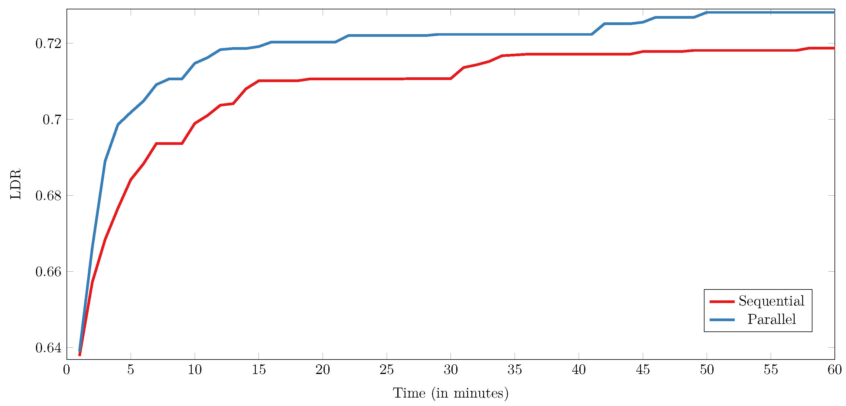
The performance of the proposed VNTS algorithm was examined across a set of real-world and synthetic benchmark instances. The results show that the algorithm performs best when the initial solution is generated with a random initialization strategy and that using parallelization leads to a significant improvement of the results in the same amount of time. By comparing the results of VNTS with those of the existing VNS-RLS algorithm from the literature, which represents the current state of the art, we found that neither algorithm consistently outperforms the other, but rather that each of the algorithms performs better for half of the instances. This shows that no single method is superior across different problems. However, it should be noted that the proposed method obtains such results in one hour, which is considerably lower than the runtime of the VNS-RLS method, which was usually an order of magnitude larger.

In future work, we plan to extend the algorithm with more complex neighborhood operators, which could help to improve the exploitation of good solutions. Furthermore, the algorithm will be extended with concepts from similar methods, such as simulated annealing or path re-linking. We also intended to extend the considered problem to include additional constraints, such as using a fleet of electric vehicles that is becoming more prominent, and adapt the algorithm to efficiently solve such problems as well. Finally, it should be noted that truck scheduling between ports is not an isolated problem, but rather is closely connected to other problems encountered in container yard terminals [34,35,36] and it is intended to consider more realistic scenarios that consider solving several of such problems jointly [37].