Stream Convolution for Attribute Reduction of Concept Lattices

Abstract

Attribute reduction is a crucial research area within concept lattices. However, the existing works are mostly limited to either increment or decrement algorithms, rather than considering both. Therefore, dealing with large-scale streaming attributes in both cases may be inefficient. Convolution calculation in deep learning involves a dynamic data processing method in the form of sliding windows. Inspired by this, we adopt slide-in and slide-out windows in convolution calculation to update attribute reduction. Specifically, we study the attribute changing mechanism in the sliding window mode of convolution and investigate five attribute variation cases. These cases consider the respective intersection of slide-in and slide-out attributes, i.e., equal to, disjoint with, partially joint with, containing, and contained by. Then, we propose an updated solution of the reduction set for simultaneous sliding in and out of attributes. Meanwhile, we propose the CLARA-DC algorithm, which aims to solve the problem of inefficient attribute reduction for large-scale streaming data. Finally, through the experimental comparison on four UCI datasets, CLARA-DC achieves higher efficiency and scalability in dealing with large-scale datasets. It can adapt to varying types and sizes of datasets, boosting efficiency by an average of 25%.

1. Introduction

In the cognitive process, people extract and define what they consider to be common features, which are called concepts. The representation of “concept” is a theory of formal concept analysis [1,2]. The concept lattice is an effective and feasible way to visualize data processing by visually representing concepts and hierarchical relationships through Hasse diagrams. In essence, the concept lattice is a binary hierarchical concept structure determined by a pair of operators, which embodies the unity of the extent and intent of the concepts. Furthermore, the generalization–specialization and partial order relations in the concept lattice implies the inclusion and partial inclusion of concepts, allowing for the extraction and application of rules. Since the introduction of formal concept analysis (FCA) in 1982, the concept lattice has been a research hotspot, including in the domains of construction [3], reduction [4], and rule extraction [5,6]. The main purpose of attribute reduction of a concept lattice is to eliminate redundant information and reduce the complexity of the concept lattice while keeping the relevant information unchanged. Attribute reduction on concept lattices can accelerate the discovery of knowledge, simplify the representation of knowledge, and ultimately reduce the number of decision rules. Therefore, it is of great theoretical and practical importance to study the attribute reduction method of the concept lattice. This method can provide powerful tools for knowledge discovery [7,8,9], data mining [10,11,12], information retrieval [13], semantic networks [14,15], and ontology construction [16,17] based on concept lattice theory.

Classical concept lattice attribute reduction algorithms are separately based on information entropy, discernibility matrix, and positive area. However, the consumption of time and space increases extremely rapidly with the increase of attributes. With the data generation changing from static to dynamic, selecting a data analysis method in a static data environment that meets the development needs can be challenging. To address this issue, Cavallero et al. [18] fully considered the reduction philosophy given in rough set theory and thus proposed a novel method of reducing attributes in fuzzy formal concept analysis. Min [19] presented the concept of soft contexts reduction and described how to extract the reduction from a given consistent set. To tackle the above-mentioned problems, Lin et al. [20] utilized a new framework for knowledge reduction in formal fuzzy contexts and developed a discernible Boolean matrix in formal fuzzy contexts by preserving extents of meet-irreducible elements via an order-class matrix. All these achievements illustrate that attribute reduction in concept lattices should be integrated with dynamism.

The integration of concept lattices and deep learning has been a topic of interest in the deep learning community. By combining concept lattices and neural networks, researchers aim to improve the accuracy of predictions and classifications. Shen et al. [21] presented a concept lattice-based neural network model. They use attribute reduction of concept lattices to extract key elements, which are then used as input for a BP neural network. Ren et al. [22] introduced an attribute reduction algorithm of concept lattices to choose attribute parameters that have good relativity to forecasting load as the input parameters of the forecasting model of neural network. This ensured the rationality of input parameters. The amalgamation of concept lattices and neural networks has further implications in the realm of data analysis. A novel algorithm, PIRA [23], leveraged dendritical neural networks to compute concept lattices, tackling the exponential complexity associated with cluster enumeration in formal concept analysis. Concept lattice theory has also been employed to tackle key challenges in neural network architecture. In order to overcome difficulties such as overfitting and poor interpretability, Kuznetsov et al. [24] proposed an approach to constructing neural networks based on concept lattices and on lattices coming from monotone Galois connections. Moreover, the utility of concept lattice theory is further seen in fields like stability prediction of rock surroundings in roadways. Liu et al. [25] employed concept lattice theory to create a prediction model with a Symmetric Alpha Stable Distribution Probability Neural Network, successfully navigating the uncertainties of multiple factors affecting roadway surrounding rock stability. Recently, concept lattices have been used to optimize graph neural networks (GNNs). Shao et al. [26] proposed a new GNN framework to improve classification accuracy by integrating concept lattice theory into the message passing of GNNs. Taken together, the research points to a promising future for the marriage of deep learning and concept lattices, heralding potential improvements in network efficiency, forecasting accuracy, data analysis, and classification performance. This integration motivates new possibilities and avenues for exploration in the field of artificial intelligence.

Convolutional neural networks (CNNs) have achieved satisfying performance in computer vision [27] and natural language processing applications [28,29] as CNN models can highly exploit the stationary and combinatorial attributes of certain types of data. Moreover, the grid nature of graphs enables the convolutional layers in CNNs to utilize hierarchical patterns to extract high-level features of graphs, resulting in a powerful representation [30]. However, the non-Euclidean nature of the graph is inappropriate for convolution and filtering of the graph learnt from images. To address the irregular shape of the spatial neighborhood, Bruna et al. [31] integrated the idea of convolution with graph computation, making a breakthrough from the spectral space and proposing a spectral network on graphs. Kipf and Welling [32] simplified Chebyshev networks by using only first-order reductions of the convolution kernel and introducing some variations to the symbols, which resulted in the creation of graph convolution networks (GCNs) [33,34,35]. GCNs are highly expressive in learning graph representations and have achieved excellent performance in a wide range of tasks and applications. Based on the above studies, we introduce the idea of convolution for large-scale attribute reduction, using a divide-and-conquer approach. Moreover, the process of CNN convolution is essentially a data preprocessing driven by divide-and-conquer, which generates the effectiveness of both data knowledge and data dimensionality reduction.

The dynamic convolution calculation is an important theoretical foundation for CNNs and GCNs. The main characteristic, as shown in Figure 1, is the two-dimensionality sliding-based calculation. Related studies [36,37] show that the CNN model is a combination of convolution calculations on different layers, whereas the GCN model is a combination of convolutional and graph calculations. Although Chen et al. [38] investigated the attribute reduction method for large-scale formal decision contexts and verified the effectiveness of the proposed algorithms, there are few studies on dynamic attribute reduction. Exploring the dynamic attribute reduction of concept lattices from the perspective of convolution calculation is challenging.

The aforementioned analyses cover FCA, concept lattice attribute reduction, and the current research status of CNN. We have identified the following challenges: Firstly, existing concept lattice attribute reduction algorithms are mainly applicable to incremental or decremental algorithms. However, simultaneous increments and decrements have not been adequately researched. Secondly, although CNN is being increasingly integrated with other fields, the research combining CNNs with concept lattices is still preliminary. Finally, a majority of neural networks merely employ the concept lattice as a deep learning data processing instrument, without genuine efforts to amalgamate the two. Based on the aforementioned challenges, we propose the dynamic convolution-based reduction calculation of concept lattice attributes. The primary contributions are as follows:

(1) This paper introduces, for the first time, the use of CNN in FCA to the attribute change mechanism of the convolutional area in the convolution calculation model. This approach not only expands the research scope of CNN but also accelerates the research progress of FCA. Specifically, The paper presents a valuable investigation of FCA in the context of CNN.

(2) This paper introduces a concept lattice attribute reduction algorithm based on dynamic convolution. The algorithm focuses on the convolution calculation model and the changing attributes of the dynamic information system in the form of attributes immigration and emigration. The proposed algorithm proves a significant improvement through the metrics of “Sig.” and “Sig. (2-tailed)” of independent samples test.

The remainder of this paper is structured as follows. Section 2 provides an overview of the relevant theories and technologies. Section 3 introduces our concept lattice modeling for convolution calculation and discusses attribute reduction reasoning and calculation. Section 4 presents the experimental results, analysis and discussions. Finally, in Section 5, we summarize the paper.

2. Preliminary

We review essential concepts of FCA here. Suppose $\left(G,M,I\right)$ is a formal context, where G is an object set, M is an attribute set, and $I\subseteq G\times M$ is a binary relation between G and M. If an object g and an attribute m have the relation I, i.e., $(g,m)\in I$, then it corresponds to the value 1 in the formal context. Otherwise, it corresponds to the value 0 in the formal context.

We firstly introduce the basic operator ∗ [1] in FCA. For $X\subseteq G$,

$$X^{*}=\left\{m|m\in M,\forall g\in X,(g,m)\in I\right\},$$

is the set of attributes that are with the relation I for all objects in X. For $B\subseteq M$,

$$B^{*}=\left\{g|g\in G,\forall m\in B,(g,m)\in I\right\},$$

is the set of objects that have relation I with all attributes in B.

Definition 1

([2]). A pair $\left(X,B\right)$ is called a formal concept or concept if $X^{*}=B$ and $B^{*}=X$. Set X is the extent of $\left(X,B\right)$, and set B is the intent of $\left(X,B\right)$. The relation between $X^{*}$ and $B^{*}$ is called a Galois connection.

Property 1 

([2]). Let $\left(X_1,B_1\right)$ and $\left(X_2,B_2\right)$ be two formal concepts, then we have:

1. 

$X_1\subseteq X_2\Rightarrow {X_2}^{*}\subseteq {X_1}^{*}$,

2. 

$B_1\subseteq B_2\Rightarrow {B_2}^{*}\subseteq {B_1}^{*}$,

3. 

$X_1\subseteq X^{**}$,

4. 

$B_1\subseteq B^{**}$,

5. 

$X_1^{*}=X_1^{***}$,

6. 

$B_1^{*}=B_1^{***}$,

7. 

$X_1\subseteq B_1^{*}\iff B_1\subseteq X_1^{*}$,

8. 

${\left(X_1\cup X_2\right)}^{*}={X_1}^{*}\cap {X_2}^{*}$,

9. 

$X_1\subseteq B_1^{*}\iff B_1\subseteq X_1^{*}$,

10. 

${\left(B_1\cup B_2\right)}^{*}={B_1}^{*}\cap {B_2}^{*}$,

11. 

${\left(X_1\cap X_2\right)}^{*}={X_1}^{*}\cup {X_2}^{*}$,

12. 

${\left(B_1\cap B_2\right)}^{*}={B_1}^{*}\cup {B_2}^{*}$.

Definition 2 

([2]). Let $K=\left(G,M,I\right)$ be a formal context, $X\subseteq G$, $B\subseteq M$. Denote the set of all concepts in context K as $L\left(K\right)$. The partial order relation on $L\left(K\right)$ is:

$$(X_1,B_1)\le (X_2,B_2)\iff X_1\subseteq X_2\iff B_1\supseteq B_2,$$

Denote $L\left(K\right)=\left(L\right(K),\le )$, as a complete lattice and is called the concept lattice of K. The supremum and infimum of the two concepts are:

$$\left(X_1,B_1\right)\wedge \left(X_2,B_2\right)=\left(X_1\cap X_2,{\left(B_1\cup B_2\right)}^{**}\right),$$

$$\left(X_1,B_1\right)\vee \left(X_2,B_2\right)=\left({\left(X_1\cup X_2\right)}^{**},B_1\cap B_2\right).$$

Before introducing the reduction of concept lattices, we define the isomorphism of lattices as a foreshadowing.

Definition 3 

([39]). Suppose that $K_1=\left(G_1,M_1,I_1\right)$ and $K_2=\left(G_2,M_2,I_2\right)$ are two formal contexts, and $L\left(K_1\right)$ with $L\left(K_2\right)$ as their corresponding concept lattices, respectively. For any $\left(X_1,B_1\right)\in L\left(K_1\right)$, if there exists $\left(X_2,B_2\right)\in L\left(K_2\right)$ such that $X_2=X_1$, then we conclude that $L\left(K_1\right)$ is finer than $L\left(K_2\right)$, denoted as $L\left(K_1\right)\le L\left(K_2\right)$.

If the formal contexts $K_1=\left(G_1,M_1,I_1\right)$ and $K_2=\left(G_2,M_2,I_2\right)$ further satisfy $L\left(K_1\right)\ge L\left(K_2\right)$ on the premise of $L\left(K_1\right)\le L\left(K_2\right)$, $L\left(K_1\right)$ is isomorphic to $L\left(K_2\right)$, denoted as $L\left(K_1\right)\cong L\left(K_2\right)$.

By the definition of isomorphism, we can further deduce the definitions of consistent set and reduction set of the concept lattice. Denote $K=(G,M,I)$ as the formal context. If the subset R of attribute set M satisfies $I_R=I\cap (G\times R)$, then $K^{\prime }=\left(G,R,I_R\right)$ is identified as the attribute sub-context of formal context $K=\left(G,M,I\right)$.

Definition 4 

([39]). Let $K=\left(G,M,I\right)$ be a formal context, and $R\subseteq M$. If $L\left(G,M,I\right)\cong L\left(G,R,I_R\right)$, then R is said to be the consistent set of $L\left(G,M,I\right)$; further, if any $D\subset R$, $L\left(G,M,I\right)\cong L\left(G,D,I_D\right)$ is not established, then R is said to be the reduction set of $L\left(G,M,I\right)$.

According to Definition 4, when the attribute sub-context forms an isomorphic relationship with the current formal context, the attribute sub-context can be considered as the coordinated set of the current formal context. If any attribute is deleted, the coordination set is no longer isomorphic to the current formal context. Consequently, this attribute sub-context is not only the coordination set of the current formal context, but also its reduction set.

Definition 5 

([39]). Let $K=\left(G,M,I\right)$ be a formal context, $(X_i,B_i)$,$(X_j,B_j)\in L(G,M,I)$, we call

$${DIS}_{FC}\left(\left(X_i,B_i\right),\left(X_j,B_j\right)\right)=B_i\cup B_j-B_i\cap B_j$$

as discernibility attributes set of $(X_i,B_i)$ and $(X_j,B_j)$. Based on this,

$${\wedge }_{FC=}({DIS}_{FC}\left(\left(X_i,B_i\right),\left(X_j,B_j\right)\right),\left(X_i,B_i\right),\left(X_j,B_j\right)\in L\left(G,M,I\right))$$

is called the discernibility matrix of the context.

According to Definition 5, we obtain the discernibility attribute matrix from the formal context. Next, we define the distinguishing function $f=\wedge \{\vee E_{i}j|E_{ij}\in {\wedge }_{FC},E_{ij}\ne \varnothing \}$ in formal context and transform function f into the disjunctive normal form $f=\left(\wedge D_1\right)\vee \left(\wedge D_2\right)\vee \dots \vee \left(\wedge D_n\right)$, where $D_i\subseteq M^{\left(t\right)}$. Every $\wedge D_t$ in the disjunctive normal form is an reduction set of the formal context. Finally, all the reduction sets $Red\left(K\right)$ of the formal context $(G,M,I)$ are obtained.

Definition 6 

([40]). Let $K=\left(G,M,I\right)$ be a formal context and $Red\left(K\right)$ be the reduction sets of $K=\left(G,M,I\right)$, then

$$\begin{array}{cc}\hfill Core& =\cap Red\left(K\right)=\left\{a|a^{*}\ne \bigcap _{\forall b_i\in M-a}{b_i}^{*}\right\}\hfill \\ \hfill RNA& =\cup Red\left(K\right)-\cap Red\left(K\right)=\left\{a|a^{*}={b_i}^{*},\exists b_i\in M-a\right\}\hfill \\ \hfill UNA& =M-\cup Red\left(K\right)=\left\{a|a^{*}=\bigcap _{\exists b_i\in M-a}{b_i}^{*}\right\}\hfill \end{array}$$

where Core is the set of core attributes, $RNA$ is the set of relative necessary attributes, and $UNA$ is the set of absolute unnecessary attributes.

The three types of attributes are represented in the formal context as the relationships between their corresponding columns. The columns corresponding to absolute unnecessary attributes can be obtained by intersecting some columns in the table. Columns corresponding to relative necessary attribute are columns corresponding to the equal columns in the table. The remaining attributes are core attributes (see

Table 1. The formal context of the student and the course $\left(G,M,I\right)$.

	a	b	c	d	e	f	h
1	0	1	1	1	0	0	0
2	1	0	0	1	1	0	1
3	1	1	0	0	1	1	0
4	0	1	0	0	0	0	1
5	1	0	0	0	1	0	0
6	1	1	0	1	1	1	0

). Due to $f^{*}=a^{*}\cap b^{*}$, attribute f is an absolute unnecessary attributes. Due to $a^{*}=e^{*}$, attribute a is a relative necessary attribute. The reduction consists of all the core attributes and some relative necessary attributes.

3. Proposed Method

3.1. Concept Lattice Modeling for Convolution Calculation

In the convolution calculation environment, the main dynamic characteristic is the sliding window that moves toward newly generated attributes. This results in both an increase and decrease in attributes. This section examines the mechanism of dynamic attribute changes in convolution calculation mode by formulating the attributes that slide into and out of the convolutional area. For simplicity, attributes that do not impact the concept lattice are filtered out and ignored in subsequent processes.

By analyzing the dynamic characteristics of convolution calculation, we can summarize the convolution calculation model into the following two change forms.

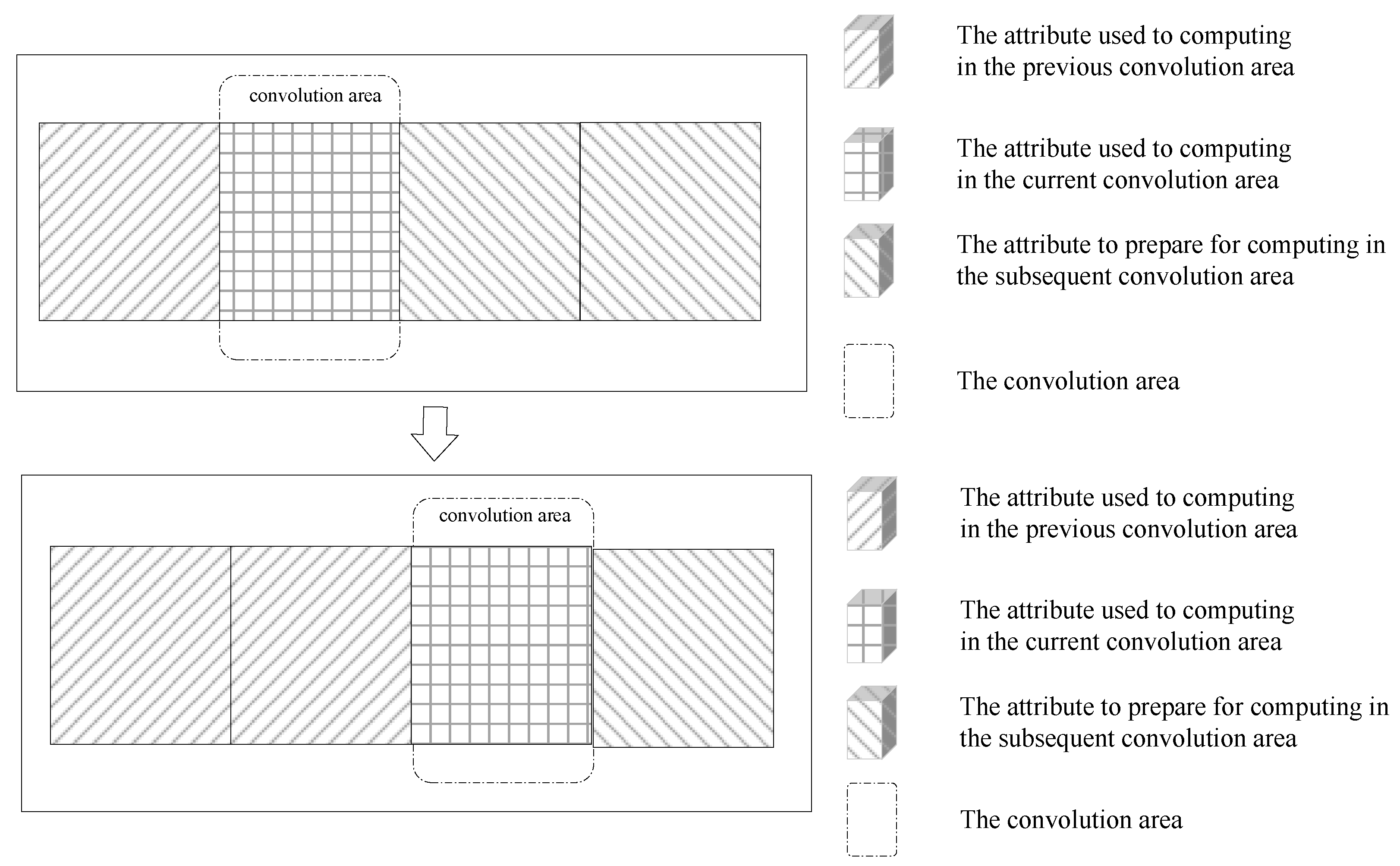
Form 1: Ordinary form. As shown in Figure 2, the individual convolutional regions slide as a sliding window. In the ordinary form, the convolutional regions slide farther apart. The new convolutional region contains only new attributes, which do not intersect with the attributes of the previous convolutional region.

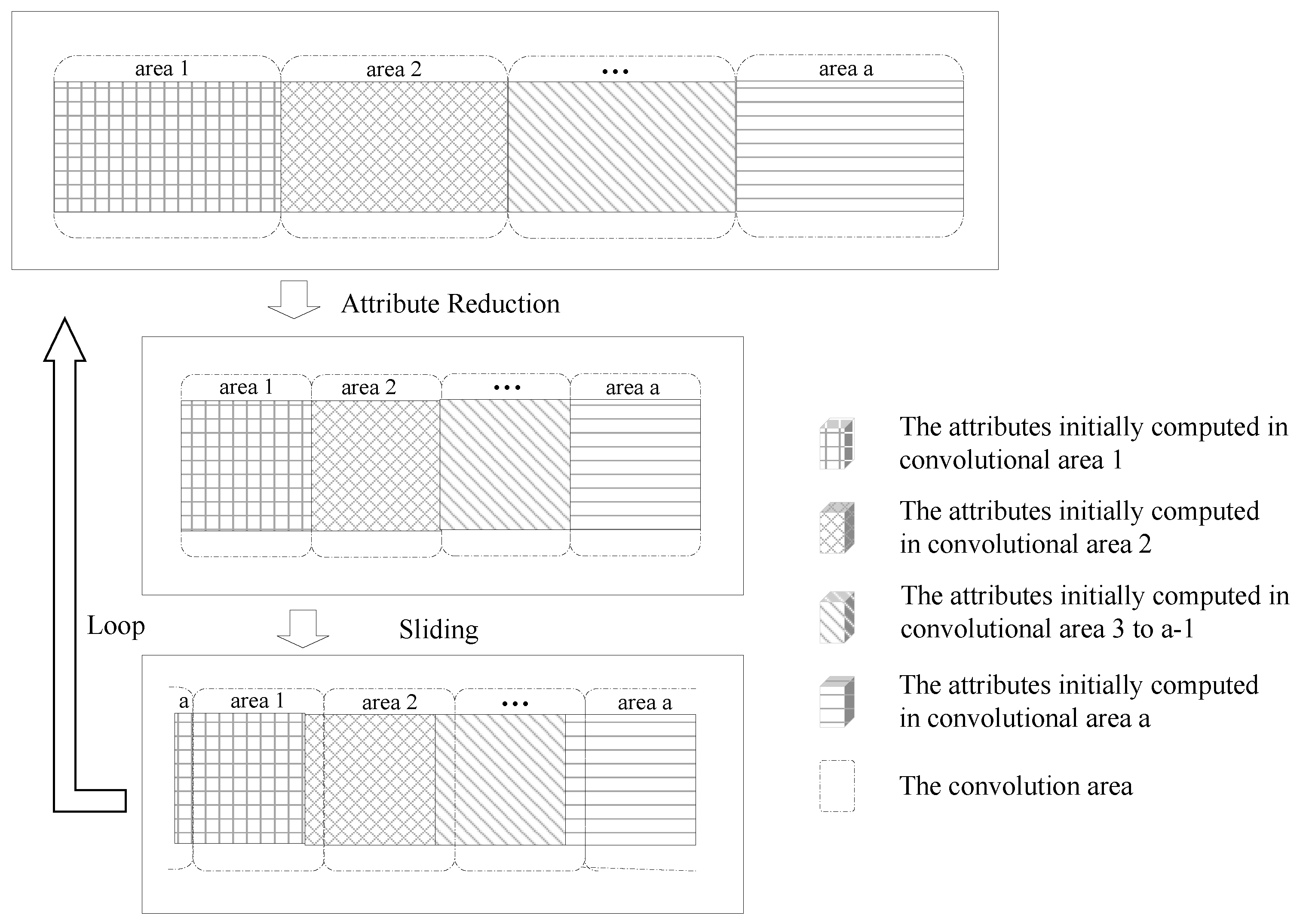
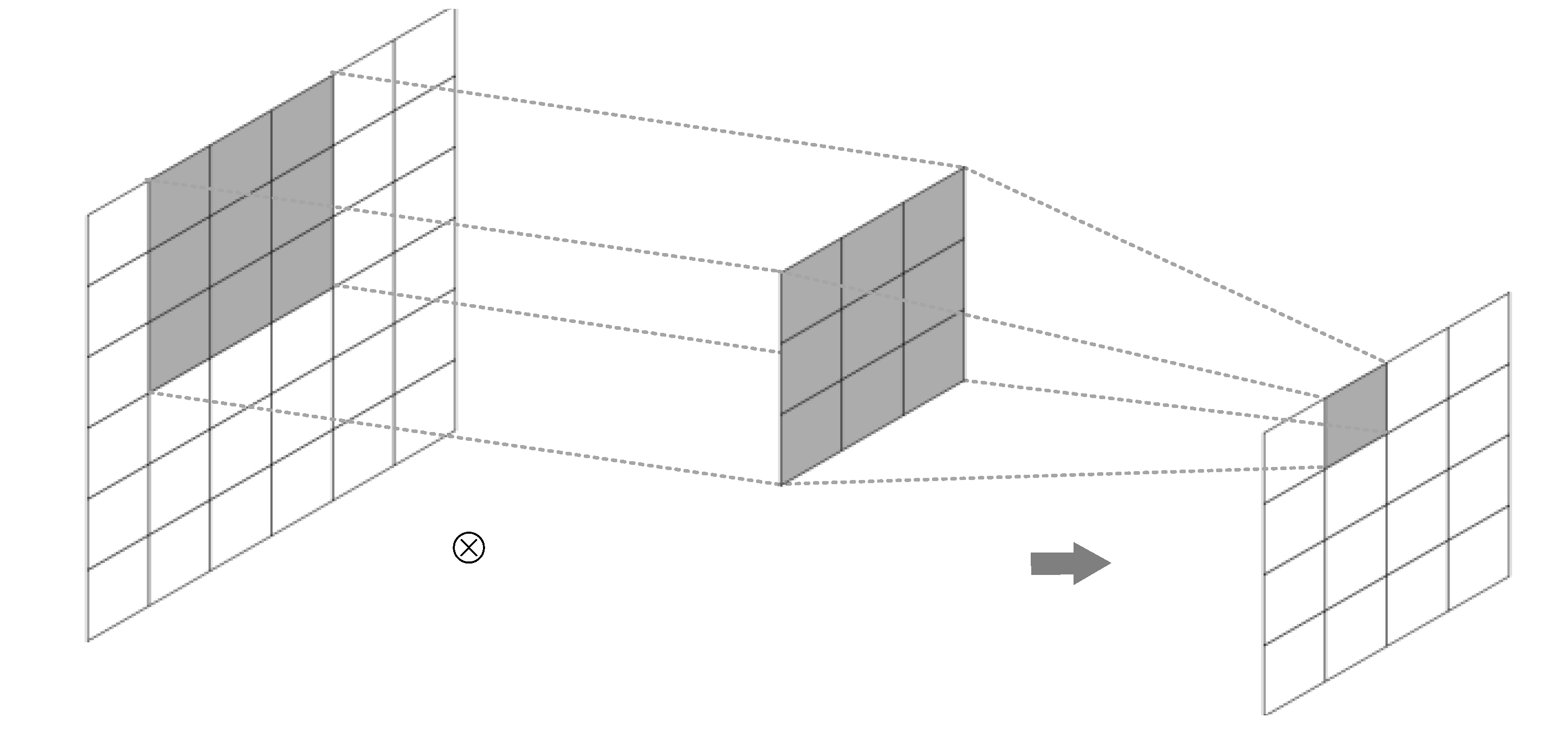
Form 2: Batch form. As shown in Figure 3, multiple convolutional regions slide a certain distance in the same direction in the form of a sliding window. In batch form, the attributes are divided into multiple convolutional regions, slide after the attribute reduction, and then the attribute reduction repeats. The current calculation window in the loop is based on the last convolutional region attribute reduction, sliding in a new batch of attributes and sliding out a small batch of old attributes.

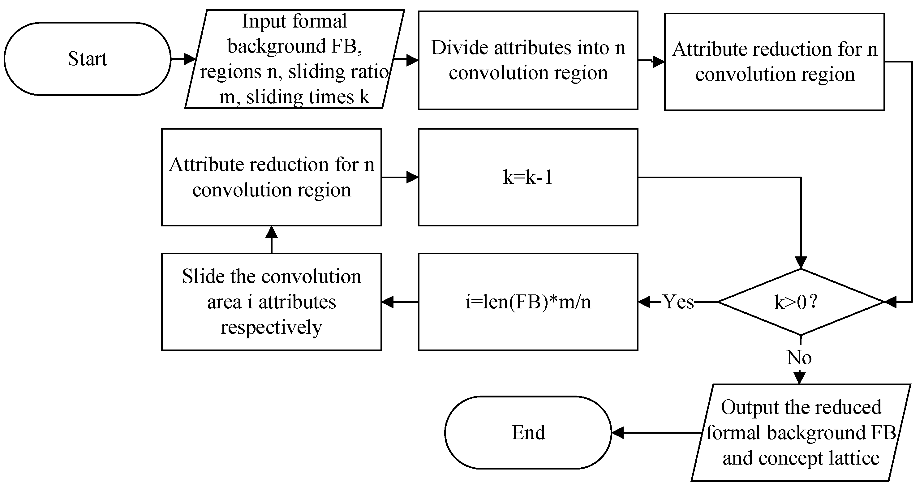
In the ordinary form of convolution calculation, only new attributes are present in the convolution area, and the old attributes are absent. This is not beneficial for studying the update of the concept lattice when attributes are incremented and decremented simultaneously. In the batch form, each time in the convolution area, a new batch of attributes is added whereas a small batch of old attributes is reduced based on the attributes left in the last adjacent convolution area. This is consistent with the dynamic characteristics of attributes that are incremented and decremented simultaneously. In what follows, we focus on the batch morphology for modeling concept lattice attributes in convolution calculation mode. The pipeline is shown in Figure 4.

In the batch form, there are five dynamic attribute changes in the convolution area, namely:

(1)

The slide-in and slide-out attributes have the same attributes.

(2)

The slide-in and slide-out attributes have the different attributes.

(3)

The slide-in and slide-out attributes partially intersect.

(4)

The slide-in attributes include the slide-out attributes.

(5)

The slide-out attributes contain the slide-in attributes.

To facilitate the discussion, we formulated the following symbolic conventions:

At time t, the formal context is denoted as $K^{\left(t\right)}=(G^{\left(t\right)},M^{\left(t\right)},I^{\left(t\right)})$, the concept lattice as $L^{\left(t\right)}=(G^{\left(t\right)},M^{\left(t\right)},I^{\left(t\right)})$, and the reduction is denoted as $R^{\left(t\right)}$. Next, in the convolution area at time t + 1, the formal context is denoted as $K^{(t+1)}=(G^{(t+1)}$,$M^{(t+1)},I^{(t+1)})$, and the concept lattice is denoted as $L^{(t+1)}=(G^{(t+1)},M^{(t+1)},I^{(t+1)})$, and the reduction is denoted as $R^{(t+1)}$.

At the time of t + 1, the attribute of sliding into the convolution area is denoted as $\overline{M}$, while the attribute of sliding out of the convolution area is denoted as $\underline{M}$. In fact, the attribute of sliding in is $\overline{M\prime }$ and the attribute of sliding out is $\underline{M\prime }$. $|\underline{M}\cap \overline{M}|$ represents the set cardinality of $\underline{M}\cap \overline{M}$. In the classical attribute reduction algorithm, it is generally assumed that $\overline{M\prime }=\overline{M}$ and $\underline{M\prime }=\underline{M}$. However, in the dynamic convolution calculation mode, we analyze its dynamic features and summarize the results in Equations (1) and (2).

$$\overline{M^{\prime }}=\left\{\begin{array}{cc}⌀,\hfill & \overline{M}=\underline{M}\hfill \\ \overline{M}-\overline{M}\cap M^{\left(t\right)},\hfill & \overline{M}\cap \underline{M}=⌀\hfill \\ ⌀,\hfill & \overline{M}\subseteq \underline{M}\hfill \\ \overline{M}-\underline{M}-\left((\overline{M}-\underline{M})\cap M^{\left(t\right)}\right),\hfill & \overline{M}\supseteq \underline{M}\hfill \\ \overline{M}-(\overline{M}\cap \underline{M})-\left((\overline{M}-(\overline{M}\cap \underline{M}))\cap M^{\left(t\right)}\right),\hfill & |\underline{M}\cap \overline{M}|<min\left(\right|\underline{M}|,|\overline{M}\left|\right)\hfill \end{array}\right.$$

(1)

$$\begin{array}{cc}\hfill & \underline{M^{\prime }}=\left\{\begin{array}{cc}⌀,\hfill & \overline{M}=\underline{M}\hfill \\ \underline{M},\hfill & \overline{M}\cap \underline{M}=⌀\hfill \\ \underline{M}-\overline{M},\hfill & \overline{M}\subseteq \underline{M}\hfill \\ ⌀,\hfill & \overline{M}\supseteq \underline{M}\hfill \\ \underline{M}-(\overline{M}\cap \underline{M}),\hfill & |\underline{M}\cap \overline{M}|<min\left(\right|\underline{M}|,|\overline{M}\left|\right)\hfill \end{array}\right.\hfill \\ \hfill & \hfill \end{array}$$

(2)

1.

When $\overline{M}=\underline{M}$, the attributes in the slide-in convolution area are the same as those in the slide-out convolution area. Suppose the order of attributes of the formal context are $a,b,c,a,b$. Given that the convolutional area contains attributes $a,b,c$, and the attributes that slide in and slide out are $a,b$ and $a,b$, respectively, then $M^{\left(t\right)}=\{a,b,c\}$, $\overline{M}=\{a,b\}$ and $\underline{M}=\{a,b\}$. We can then reason that $\overline{M^{\prime }}=⌀$ and $\underline{M^{\prime }}=⌀$, which finally yields $M^{(t+1)}=M^{\left(t\right)}\cup \overline{M^{\prime }}-\underline{M^{\prime }}=\{c,a,b\}$.

2.

When $\overline{M}\ne \underline{M}$, the attributes in the slide-in convolution area have four different representations from those in the slide-out convolution area.

(a)

When $\overline{M}\cap \underline{M}=\varnothing$, the attributes in the slide-in convolution area are completely different from those in the slide-out convolution area at this time. Suppose the order of attributes of the formal context are $a,b,e,d,e$. Given that the convolutional area contains attributes $a,b,c$, and the attributes that slide in and slide out are $a,b$ and $d,e$, respectively, then $M^{\left(t\right)}=\{a,b,e\}$, $\overline{M}=\{d,e\}$ and $\underline{M}=\{a,b\}$. We can then reason that $\overline{M}\cap M^{\left(t\right)}=\left\{e\right\},$ $\overline{M^{\prime }}=\overline{M}-\overline{M}\cap M^{\left(t\right)}=\left\{d\right\}$ and $\underline{M^{\prime }}=\underline{M}=\{a,b\}$, which finally yields $M^{(t+1)}=M^{\left(t\right)}\cup \overline{M^{\prime }}-\underline{M^{\prime }}=\{d,e\}$.

(b)

When $\overline{M}\subseteq \underline{M}$, the attribute that slides out of the convolution area at this time contains the attribute that slides into the convolution area. Therefore, compared with the attributes in the convolution area at the time t, there is actually no slide-in attribute, but a slide-out attribute $\underline{M}-\overline{M}$. Suppose the order of attributes in the formal context is $a,b,c,a,a$. Given that the convolutional area contains attributes $a,b,c$, and the attributes that slide in and slide out are $a,a$ and $a,b$, respectively, then $M^{\left(t\right)}=\{a,b,c\}$, $\overline{M}=\left\{a\right\}$ and $\underline{M}=\{a,b\}$. We can then reason that $\overline{M^{\prime }}=⌀$ and $\underline{M^{\prime }}=\underline{M}-\overline{M}=\left\{b\right\}$, which finally yields $M^{(t+1)}=M^{\left(t\right)}\cup \overline{M^{\prime }}-\underline{M^{\prime }}=\{c,a\}$.

(c)

When $\overline{M}\supseteq \underline{M}$, the attribute sliding into the convolution area at this time contains the attribute sliding out of the convolution area. Therefore, compared with the attributes in the convolution area at time t, there are actually no sliding-out attributes, but rather sliding-in attributes $\overline{M}-\underline{M}$. Suppose the order of attributes in the formal context is $a,a,a,b,c,b,a$. Given that the convolutional area contains attributes $a,a,a,b$, and the attributes that slide in and slide out are $c,b,a$ and $a,a,a$, respectively, then $M^{\left(t\right)}=\{a,b\}$, $\overline{M}=\{c,b,a\}$, $\underline{M}=\left\{a\right\}$. We can then reason that $\underline{M^{\prime }}=⌀$. $(\overline{M}-\underline{M})\cap M^{\left(t\right)}=\left\{b\right\}$ means a property that is present in $\overline{M}$ but not in $\underline{M}$, and which may have originally existed in $M^{\left(t\right)}$. Therefore, $\overline{M}-\underline{M}-\left((\overline{M}-\underline{M})\cap M^{\left(t\right)}\right)=\left\{c\right\}$, which leads to $M^{(t+1)}=M^{\left(t\right)}\cup \overline{M^{\prime }}-\underline{M^{\prime }}=\{c,b,a\}.$

(d)

When $|\underline{M}\cap \overline{M}|<min(|\underline{M}|,|\overline{M}\left|\right)$, the attributes in the slide-in convolution area partially intersect with the attributes in the slide-out convolution area. Suppose the order of attributes of the formal context are $a,b,c,d,e,d,a$. Given that the convolutional area contains attributes $a,b,c,d$, and the attributes that slide in and slide out are $e,d,a$ and $a,b,c$, respectively, then $M^{\left(t\right)}=\{a,b,c,d\}$, $\overline{M}=\{e,d,a\}$ and $\underline{M}=\{a,b,c\}$. We can then reason that $\underline{M^{\prime }}=\underline{M}-(\overline{M}\cap \underline{M})=\{b,c\}$. The reason for subtracting $(\overline{M}-(\overline{M}\cap \underline{M}))\cap M^{\left(t\right)}=\left\{d\right\}$ is to prevent $\overline{M}$ from adding the attributes that $M^{\left(t\right)}$ already contains. Therefore, $\overline{M}-(\overline{M}\cap \underline{M})-\left((\overline{M}-(\overline{M}\cap \underline{M}))\cap M^{\left(t\right)}\right)=\left\{e\right\}$, which leads to $M^{(t+1)}=M^{\left(t\right)}\cup \overline{M^{\prime }}-\underline{M^{\prime }}=\{e,d,a\}.$

Further analysis is conducted to determine whether any of the attributes that slide into the convolutional area already exist or not in the convolutional area at time t. If some attributes already exist in the convolution area at time t, they do not affect the result when they slide into the convolution window. These partially overlapping attributes, represented as $\overline{M}-\overline{M}\cap M^{\left(t\right)}$, should be removed.

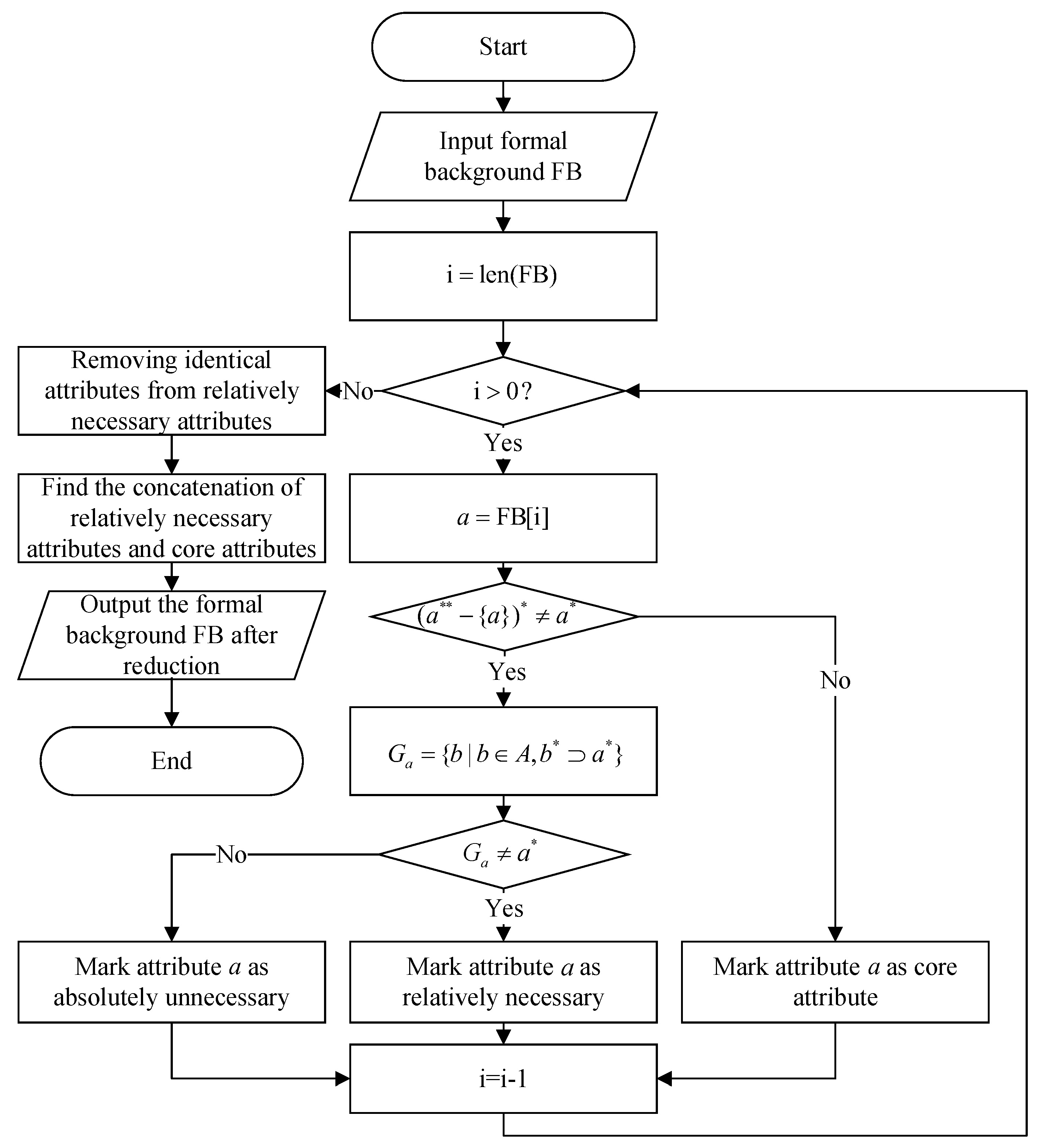
The concept lattice reduction based on the new difference matrix requires regenerating the concept and repeatedly performing merge operations at each slide. This results in excessive redundancy in the calculation process and disqualification for the convolution calculation model. The concept lattice reduction algorithm based on attribute features is a classical attribute reduction algorithm with excellent performance compared to other algorithms. Under the requirements ${\left(a^{**}-a\right)}^{*}\ne a^{*}$ and $G_a=\left\{b\right|b\in A,b^{*}\subset a^{*}\}$, we can compute core and relative necessary and absolute unnecessary attributes with a time complexity of $O\left(\right|M{|}^2)$. The algorithm flow chart based on attribute characteristics is shown in Figure 5.

3.2. Attribute Reduction Reasoning in Convolution Calculation

We investigate the influence of slide-in and slide-out attributes on the reduction set $Red\left(K\right)$ with the formal context $K=(G,M,I)$ and summarize the rules.

When adding an attribute, we compare and analyze its effect on the reduction result with the concept lattice. First, we identify the type of attribute, i.e., a core attribute, a relative necessary attribute, and an absolute unnecessary attribute. Then, we investigate how each type of attribute will be affected by adding that type of attribute to the concept lattice. Finally, we obtain Theorems 1–3.

Theorem 1. 

Let $K=(G,M,I)$ be the formal context, R the reduction of K, and a the attribute to be added. If $a^{*}={\bigcap }_{\exists b_i\in M}{b_i}^{*}$, then the reduction remains the same as R.

Proof. 

Since $a^{*}={\bigcap }_{\exists b_i\in M}{b_i}^{*}$, it is clear from Definition 6 that the added attribute a is unnecessary. Therefore, the added unnecessary attribute has no effect on the result of the reduction, which means the reduction remains unchanged.    □

Theorem 2. 

Let $K=(G,M,I)$ be the formal context, R the reduction of K, and a the attribute to be added. If there exists an attribute $b_i\in M$ such that $a^{*}={b_i}^{*}$, then the reduction R remains unchanged.

Proof. 

Since $b_i\in M$, $a^{*}={b_i}^{*}$, according to Definition 6, it is known that the added attribute a is a relative necessary attribute. Since $a^{*}={b_i}^{*}$, regardless of whether $b_i$ belongs to R, the added relative necessary attribute a has no effect on the reduction result, and thus the reduction remains unchanged.    □

Theorem 3. 

Let $K=(G,M,I)$ be the formal context, R the reduction of K, and a the attribute to be added. If $a^{*}\ne {\bigcap }_{\forall b_i\in M}{b_i}^{*}$, and there is no $d\in R$ such that $d^{*}={b_i}^{*}\cap a^{*}$, there exists $b_i\in M$, then the reduction is updated to $R\cup a$. Conversely, if there exists $d\in R$, such that $d^{*}={b_i}^{*}\cap a^{*}$, there exists $b_i\in M$, then the reduction is updated to $(R-d)\cup \left\{a\right\}$.

Proof. 

Since $a^{*}\ne {\bigcap }_{\forall b_i\in M}{b_i}^{*}$, it follows Definition 6 that the added attribute a is the core attribute.

If $\forall d\in R$ such that $d^{*}={b_i}^{*}\cap a^{*}$, there exists $b_i\in M$, the reduction result is updated to $R\cup \left\{a\right\}$.

If there exists $d\in R$, satisfying $d^{*}={b_i}^{*}\cap a^{*}$, there exists $b_i\in M$, it means that the addition of attribute a causes the attribute d in the previous reduction results to become an unnecessary attribute. Therefore, d needs to be removed from R, so the reduction result is updated to $\left(R-d\right)\cup \left\{a\right\}$.    □

The process for deleting an attribute is analogous. First, we determine the attribute type, i.e., a core attribute, a relative necessary attribute, or an absolute unnecessary attribute. Then, we investigate whether the attribute is already present in the result. If it holds, we remove it from the result and reanalyze whether the attributes of associated attributes have changed after its deletion. Otherwise, we analyze whether its deletion will impact the reduction result. Based on these changes, we summarize Theorems 4–6.

Theorem 4. 

Let $K=(G,M,I)$ be the formal context, R the reduction of K, and attribute a the attribute to be deleted. If $a^{*}={\bigcap }_{\exists b_i\in M-a}{b_i}^{*}$, then the reduction remains R.

Proof. 

Since $a^{*}={\bigcap }_{\exists b_i\in M-a}{b_i}^{*}$, it is clear from Definition 6 that the deleted attribute a is unnecessary. Therefore, the deleted unnecessary attribute a has no effect on the reduction, i.e., the reduction R remains unchanged.    □

Theorem 5. 

Let $K=(G,M,I)$ be the formal context, R the reduction of K, and attribute a the attribute to be deleted. If $a^{*}\ne {\bigcap }_{\forall b_i\in M-a}{b_i}^{*}$ and there is no $d\in M-R$ such that $d^{*}\ne {\bigcap }_{\forall b_i\in M-a-d}{b_i}^{*}$, or $d^{*}=\left({\bigcap }_{\exists b_i\in M-a-d}{b_i}^{*}\right)\cap a^{*}$, then the reduction is updated to $R-a$. Conversely, if $a^{*}\ne {\bigcap }_{\forall b_i\in M-a}{b_i}^{*}$ and there exists $d\in M-R$, such that $d^{*}\ne {\bigcap }_{\forall b_i\in M-a-d}{b_i}^{*}$, or $d^{*}=\left({\bigcap }_{\exists b_i\in M-a-d}{b_i}^{*}\right)\cap a^{*}$, then the reduction is updated to $\left(R-a\right)\cup \left\{d\right\}$.

Proof. 

Since $a^{*}\ne {\bigcap }_{\forall b_i\in M-a}{b_i}^{*}$, it follows from Definition 6 that the deleted attribute a is the core attribute.

If $a^{*}\ne {\bigcap }_{\forall b_i\in M-a}{b_i}^{*}$ and there is no $d\in M-R$, such that either $d^{*}\ne {\bigcap }_{\forall b_i\in M-a-d}{b_i}^{*}$ or $d^{*}=\left({\bigcap }_{\exists b_i\in M-a-d}{b_i}^{*}\right)\cap a^{*}$ holds, then the attribute a degenerates from core to unnecessary, which means the reduction is updated to $R-a$.

If there exists $d\in M-R$ such that $d^{*}\ne {\bigcap }_{\forall b_i\in M-a-d}{b_i}^{*}$, it means that there is a new core attribute d generated after removing attribute a. Therefore, the reduction is updated to $\left(R-a\right)\cup \left\{d\right\}$.

If there exists $d\in M-R$, such that $d^{*}=\left({\bigcap }_{\exists b_i\in M-a-d}{b_i}^{*}\right)\cap a^{*}$, it means that d is originally an unnecessary attribute. After removing attribute a, $d^{*}\ne {\bigcap }_{\forall b_i\in M-a-d}{b_i}^{*}$, attribute d becomes the new core attribute, therefore it is necessary to add attribute d to the reduction result, i.e., the reduction is updated to $\left(R-a\right)\cup \left\{d\right\}$.    □

Theorem 6. 

Let $K=\left(G,M,I\right)$ be a formal context, R the reduction of K, and a the attribute to be deleted. If $a\in R$, there exists $b_i\in M$ such that $a^{*}={b_i}^{*}$, then the reduction update is $\left(R-a\right)\cup \left\{b_i\right\}$. Conversely, if $a\in M-R$, there exists $b_i\in M$ such that $a^{*}={b_i}^{*}$, then the reduction remains the same still as R. Let R be the reduction of K, and a is the attribute to be deleted. If $a\in R$, there exists $b_i\in M$ such that $a^{*}={b_i}^{*}$, then the reduction is updated to $\left(R-a\right)\cup \left\{b_i\right\}$. Conversely, if $a\in M-R$, there exists $b_i\in M$ such that $a^{*}={b_i}^{*}$, then the reduction remains the unchanged.

Proof. 

Since there exists $b_i\in M$, such that $a^{*}={b_i}^{*}$, it follows from Definition 6 that the deleted attribute a is relative necessary.

If $a\in R$, it means that the deletion of attribute a has effects on the existing reduction result. Since $a^{*}={b_i}^{*}$, then $b_i$ replaces a in R, generating a reduction with constant number, i.e., the reduction is updated to $\left(R-a\right)\cup \left\{b_i\right\}$.

If $a\in M-R$, it means that deleting the attribute a will have no effects on the existing reduction result, and thus the reduction remains unchanged.    □

3.3. Complexity Analysis

Based on the theoretical study, a concept lattice attribute reduction algorithm for dynamic convolution is designed. Section 3.1 and Section 3.2 investigate the dynamic attribute change mechanism and related theorems concerning dynamic attribute reduction in the convolution calculation model. The goal is to address the attribute reduction issue of the concept lattice, characterized by both incremental and decremental attribute reduction. Algorithm 1 proposes a concept lattice attribute reduction algorithm based on dynamic convolution (CLARA-DC). The classical attribute reduction algorithm does not apply to the case where attributes are incremental and decremental at the same time. It not only ignores the connection between the slide-in and slide-out attributes but also recomputes all attributes, and thus the time complexity is $O\left(\right(\left|M\right|+{\left|N\right|)}^2)$. $\left|M\right|$ and $\left|N\right|$ refer to the number of initial attributes and the number of added attributes, respectively. CLARA-DC uncovers the connection between the slide-in attributes, slide-out attributes, and the initial attributes before the reduction through Equations (1) and (2) in Step 1 and processes them in advance, thus avoiding unnecessary computations. Meanwhile, CLARA-DC only needs to compare the actual slide-in attributes and the initial attributes, and the time complexity is $O\left(\right(\left|N\right|+\left|M\right|)\times |N\left|\right)$.

3.4. Example of CLARA-DC

Table 1 shows the formal context $\left(G,M,I\right)$ for “students and courses”, where the set of student objects G consists of objects 1, 2, 3, 4, 5, 6; the set of attributes M consists of seven attributes: a, b, c, d, e, f, h. If $\left(G,M\right)\in I$, then the student has the course and it is marked as 1 in the table; if $\left(G,M\right)\notin I$, i.e., the student does not have the course, then it is marked as 1 in the table; in the convolution area at time t, it contains only attributes a, b, c, d, e. However, as the convolution window slides, at time t + 1, attributes d, e, f, h slide into the convolution area, while attributes a, c, d, e slide out of the convolution area.

According to Definition 1, we obtain the concept of the corresponding form of data in the convolutional area at time t. For instance, Object 1 has attributes b, c, and d, and only Object 1 contains all three attributes. According to Definition 1, this is shown in Table 1.

We know that $\left(1,bcd\right)$ is a formal concept; Object 2 has attributes a, d, e, but Objects 2 and 6 also contain the attributes a, d, e. Therefore, $\left(2,ace\right)$ is not a formal concept according to Definition 1. All formal concepts are thus determined according to Definition 1, as shown in

Table 2. Formal concepts corresponding to the formal contexts in Table 1.

Label	Concept	Label	Concept
$C_1$	$\left(\varnothing ,abcde\right)$	$C_6$	$\left(36,abe\right)$
$C_2$	$\left(1,bcd\right)$	$C_7$	$\left(126,d\right)$
$C_3$	$\left(6,abde\right)$	$C_8$	$\left(1346,b\right)$
$C_4$	$\left(16,bd\right)$	$C_9$	$\left(2356,ae\right)$
$C_5$	$\left(26,ade\right)$	$C_{10}$	$\left(\mathrm{123,456},\varnothing \right)$

.

Algorithm 1 CLARA-DC

Input:  At time t, $K^{\left(t\right)}=\left(G^{\left(t\right)},M^{\left(t\right)},I^{\left(t\right)}\right)$ is the formal context and reduction result is $R^{\left(t\right)}$. At time t + 1, the attribute $\overline{M}$ of sliding into the convolution area and the attribute $\underline{M}$ of sliding out of the convolution area. Output:  At the time of t + 1, the reduction result $R^{(t+1)}$. 1: Step 1: According to Equations (1) and (2), the actual sliding-in and sliding-out attributes of t + 1 are computed, namely, $\overline{M^{\prime }}$ and $\underline{M^{\prime }}$. 2: Step 2: Iterate over the actual slide-in attribute $\overline{M^{\prime }}$, denoting one of the attributes by a. According to Theorems 1–3, $R^t$ is updated. Define $R^{\prime }=R^t$. 3:        Step 2.1: If $a^{*}={\bigcap }_{\exists b_i\in M}{b_i}^{*}$, then $R^{\prime }=R^{\prime }$. 4:        Step 2.2: If there exists $b_i\in M$, such that $a^{*}={b_i}^{*}$, then $R^{\prime }=R^{\prime }$. 5:        Step 2.3: If $a^{*}\ne {\bigcap }_{\forall b_i\in M}{b_i}^{*}$ and there are no $d\in R^{\left(t\right)}$ such that $d^{*}=\left({\bigcap }_{\exists b_i\in M}{b_i}^{*}\right)\cap a^{*}$, then $R^{\prime }=R^{\prime }\cup \left\{a\right\}$. 6:        Step 2.4: If $a^{*}\ne {\bigcap }_{\forall b_i\in M}{b_i}^{*}$ and there exists $d\in R^{\left(t\right)}$ such that $d^{*}=\left({\bigcap }_{\exists b_i\in M}{b_i}^{*}\right)\cap a^{*}$, then $\left(R^{\left(t\right)}-d\right)\cup \left\{a\right\}$. 7:        Step 2.5: Return to step 2 and take the next attribute of $\overline{M^{\prime }}$. Until all the attributes in $\overline{M^{\prime }}$ are added to get the new reduction $R^{\prime }$, go to step 3. 8: Step 3: Iterate over the actual slide-out attribute $\underline{M^{\prime }}$, and denote one of the attributes by a. According to Theorems 4–6, $R^{\prime }$ is updated. 9:        Step 3.1: If $a^{*}={\bigcap }_{\exists b_i\in M-a}{b_i}^{*}$, then $R^{\prime }=R^{\prime }$. 10:      Step 3.2: If $a^{*}\ne {\bigcap }_{\forall b_i\in M-a}{b_i}^{*}$ and there is no $d\in M-R^{\prime }$ such that $d^{*}\ne {\bigcap }_{\forall b_i\in M-a-d}{b_i}^{*}$ or $d^{*}=\left({\bigcap }_{\exists b_i\in M-a-d}{b_i}^{*}\right)\cap a^{*}$, then $R^{\prime }=R^{\prime }-a$. 11:      Step 3.3: If $a^{*}\ne {\bigcap }_{\forall b_i\in M-a}{b_i}^{*}$ and there exists $d\in M-R^{\prime }$ such that $d^{*}\ne {\bigcap }_{\forall b_i\in M-a-d}{b_i}^{*}$ or $d^{*}=\left({\bigcap }_{\exists b_i\in M-a-d}{b_i}^{*}\right)\cap a^{*}$, then $R^{\prime }=\left(R^{\prime }-a\right)\cup \left\{d\right\}$. 12:      Step 3.4: There exists $b_i\in M$ such that $a^{*}={b_i}^{*}$. If $a\in R^{\prime }$, then $R^{\prime }=\left(R^{\prime }-a\right)\cup \left\{b_i\right\}$. However, if $a\in M-R^{\prime }$, then $R^{\prime }=R^{\prime }$. 13:      Step 3.5: Return to Step 3 and take the next attribute of $\underline{M^{\prime }}$, until all the attributes in $\underline{M^{\prime }}$ are deleted. 14: Step 4: Output $R^{\left(t+1\right)}$.

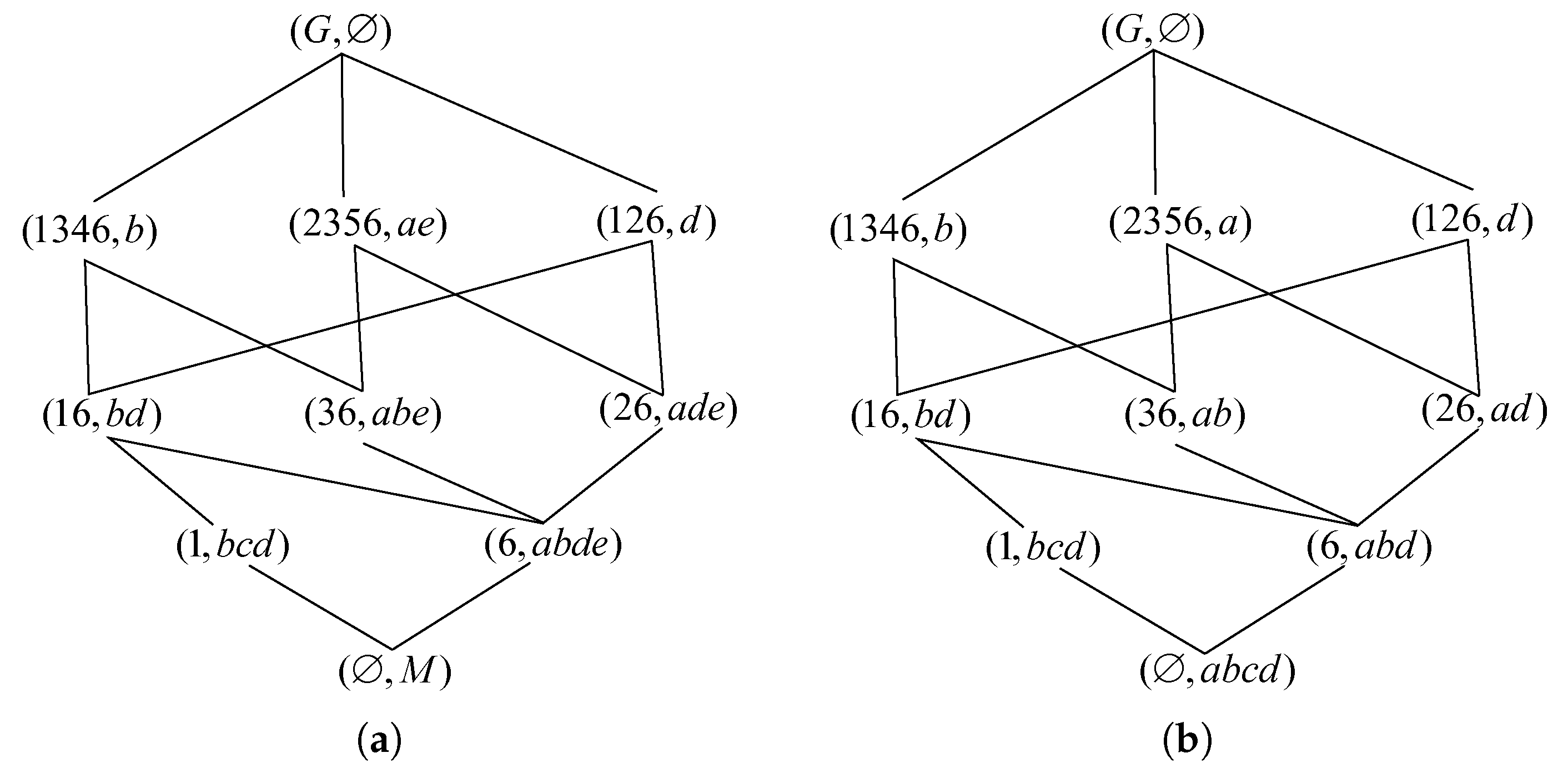
Formal concepts have certain partial order relations, and the concept lattice corresponding to the formal context at the time t is shown in Figure 6a. According to Definition 6, in the formal context, the core attributes are b, c, d and the relative necessary attributes are a, e. One of the attribute reductions is $R=\{a,b,c,d\}$. The concept lattice corresponding to the time t is shown in Figure 6b.

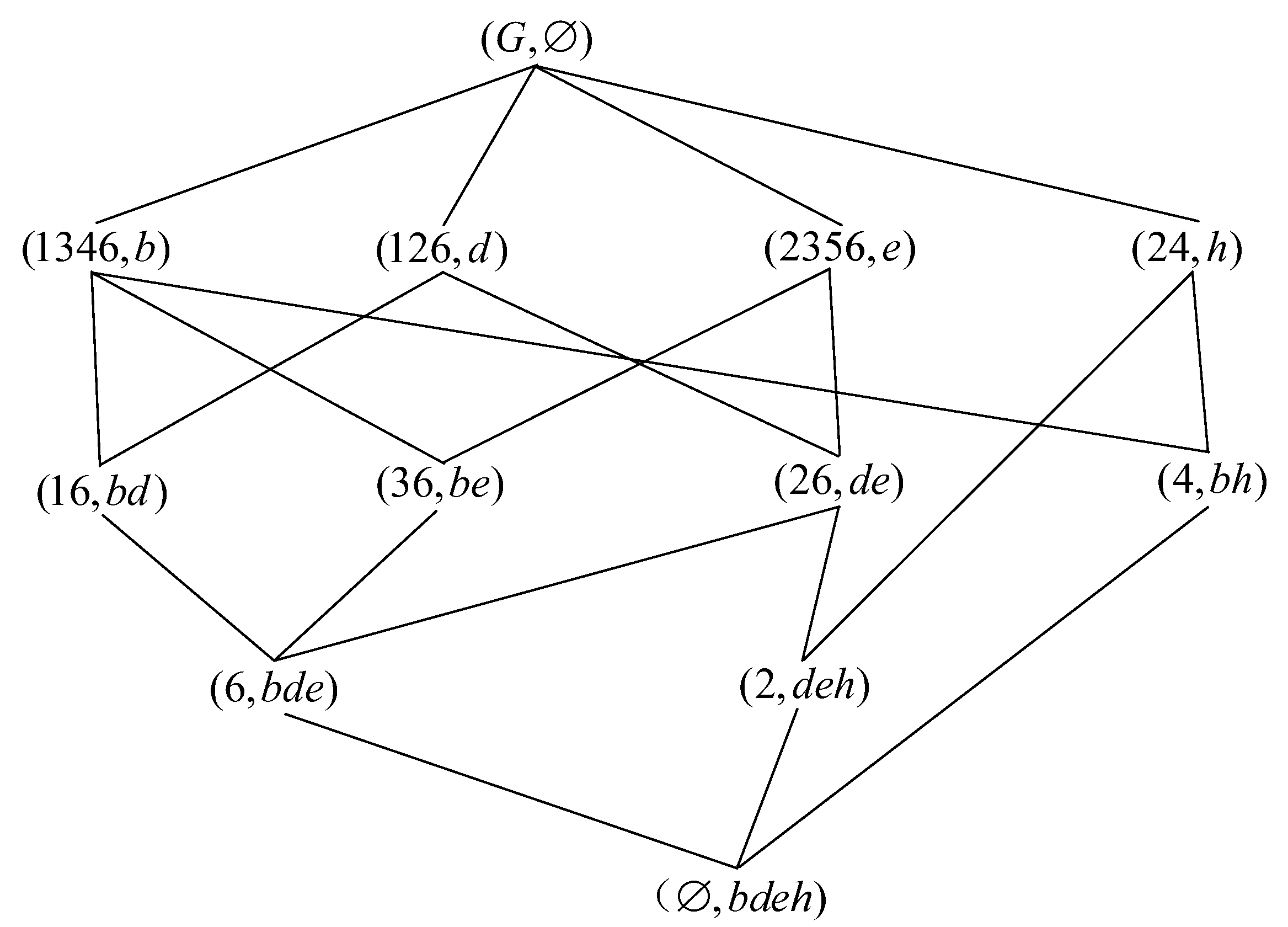
At time t + 1, the attributes sliding into the convolution area are d, e, f, h and the attributes sliding out of the convolution area are a, c, d, e. According to the CLARA-DC algorithm, the update reduction $R=\{a,b,c,d\}$.

Compute the actual slide-in and slide-out attributes f, h and a, c at time t + 1 according to the Equations (1) and (2). The attributes f, h are related to the objects $\left(36,f\right)$, $\left(24,h\right)$.

The attribute f is an unnecessary absolute attribute since $f^{*}=a^{*}\cap b^{*}$. Adding the attribute f has no effects on the reduction, and thus the result of the reduction remains unchanged, denoted as $R^{\prime }=R=\{a,b,c,d\}$.

For attribute h, since $h^{*}\ne {\bigcap }_{\forall b_i\in M}{b_i}^{*}$, and there is no $d\in R^{\prime }$ such that $d^{*}={b_i}^{*}\cap h^{*}$, there exists $b_i\in M$, and thus attribute h is a core attribute, $R^{\prime }=\{a,b,c,d,h\}$.

For attribute a, since there is $a\in R^{\prime }$ and there is $e\in M-R^{\prime }$ to make $a^{*}=e^{*}$, attribute a is thus a relative necessary attribute. Replacing e with a in $R^{\prime }$ means that the reduction is updated to $R^{\prime }=\left(R^{\prime }-a\right)\cup e=\{b,c,d,e,h\}$.

For attribute c, since $c^{*}\ne {\bigcap }_{\forall b_i\in M-c}{b_i}^{*}$ and there is no $d\in M-R^{\prime }$, such that $d^{*}\ne {\bigcap }_{\forall b_i\in M-a-d}{b_i}^{*}$ or $d^{*}=\left({\bigcap }_{\exists b_i\in M-a-d}{b_i}^{*}\right)\cap a^{*}$, and thus attribute c is an absolute unnecessary attribute, then the reduction is updated to $R^{\prime }=R^{\prime }-c=\{b,d,e,h\}$

The output is $R^{\prime }=\{b,d,e,h\}$. The corresponding concept lattice is shown in Figure 7.

4. Experimental Analysis

4.1. Settings

The efficiency of the algorithm is verified by comparing the running time of the algorithm. Four datasets from the UCI database (http://archive.ics.uci.edu/ml/datasets, accessed on 3 August 2022) are selected for the experiment. The basic information of these datasets is shown in

Table 3. Comparisons between classical attribute reduction algorithm and CLARA-DC.

	Nurs	Mush	AMWD	T-Mush
$\left|G\right|\times \left|M\right|$	$12,960\times 30$	$8124\times 115$	$32,710\times 30$	$115\times 8124$
Concepts	154,005	233,101	129,009	233,101
Classic [39]	0.997 ms	7.718 ms	158.643 ms	17.541 s
CLARA-DC	1.002 ms	5.556 ms	96.286 ms	11.437s

. All data are processed by binary and dummy variables. The experimental platform is Windows 11, the CPU is Intel i5-9400F, the memory is 16 GB, the language is Python, and the coding software is PyCharm 2022. All experimental results are repeated five times, and the average values are reported. The time function in the time module in Python calculates the running time of a program with an accuracy down to the microsecond level. We use it to obtain the running time of the model for the conceptual lattice reduction.

4.2. Results

We compare the time consumed by the CLARA-DC algorithm and the classical attribute reduction algorithm proposed in the paper [39] on four datasets. Nursery, Mushroom, Anonymous Microsoft Web Data, and Transposed Mushroom are respectively abbreviated as Nurs, Mush, AMWD, and T-Mush.The results are shown in Table 3.

As shown in Table 3 and Figure 8, the proposed CLARA-DC is more efficient than the classical reduction algorithm. The units in Figure 8a–c are milliseconds, whereas the units in Figure 8d are seconds.

We first examine the normality of the experimental results on different datasets from

Table A1. Raw results for classical attribute reduction algorithm and CLARA-DC.

	Nurs (ms)	Mush (ms)	AMWD (ms)	T-Mush (s)
Classical	0.997	7.632	146.640	17.461
	0.999	7.342	168.620	16.972
	0.995	7.696	173.015	18.557
	0.997	7.903	156.290	18.326
	0.997	8.017	148.650	16.391
CLARA-DC	1.002	6.480	90.790	11.431
	1.003	5.980	98.770	11.301
	1.003	5.260	97.794	11.211
	1.000	4.980	103.320	11.579
	1.002	5.080	90.756	11.663

and find that it basically conforms to normal distribution. Therefore, we performed the independent samples test by SPSS software to obtain the following metrics, which are “F” and “sig.” in Levene’s test, and “t”, “df”, “Sig. (2-tailed)” and “Mean Difference” in t-test for equality of means. In Levene’s test for equality of variances, “F” represents the test statistic. It is the ratio of the between-groups variability to the within-groups variability. A larger F value indicates a larger difference in variances among the groups. In t-test, “Sig.” stands for significance, which is the p-value associated with the “F” statistic. It indicates the probability of obtaining the observed data that variances between the compared results are statistically equal (the null hypothesis) holds. If the p-value (Sig.) is less than the chosen significance level ($\alpha =$ 0.05), we can conclude that there are significant differences in the variances across groups. “t” is the test statistic. It measures how much the groups differ by standardizing variability of the two groups. A larger absolute value of t indicates a larger difference between the groups relative to the variability within the groups.“df” stands for degrees of freedom, which is the expected number of independent pieces. In the context of a t-test, it is typically the total sample size across all groups minus the number of groups. “Sig. (2-tailed)” represents the p-value for a two-tailed t-test. It estimates the probability of observing the lower and upper bound of mean value in the compared groups are statistically equal under the t-distribution (the null hypothesis). If the p-value is less than the chosen significance level ($\alpha =$ 0.05), we would reject the null hypothesis and conclude that there is a significant difference between the means of the groups. “Mean Difference” is the difference between the means of the two groups being compared. It illustrates how much the groups differ in terms of their means. The sign of the mean difference reveals the direction of this difference.

By comparing different datasets in

Table 4. Independent samples test between classical attribute reduction algorithm and CLARA-DC.

		F	Sig.	t	df	Sig. (2-Tailed)	Mean Difference
Nurs	Equal variances assumed	0.000	1.000	−5.976	8	<0.001	−0.005
	Equal variances not assumed			−5.976	7.840	<0.001	−0.005
Mush	Equal variances assumed	7.673	0.024	6.920	8	<0.001	2.162
	Equal variances not assumed			6.920	5.266	<0.001	2.162
AMWD	Equal variances assumed	5.530	0.047	10.739	8	<0.001	62.357
	Equal variances not assumed			10.739	5.635	<0.001	62.357
T-Mush	Equal variances assumed	8.857	0.018	14.715	8	<0.001	6.104
	Equal variances not assumed			14.715	4.341	<0.001	6.104

, we find that the “Sig.” of the datasets Mush, AMWD, and T-Mush are all less than 0.05, which means that the experimental results of the two algorithms on these datasets are significantly different in terms of variance. Then, we should check the “Sig. (2-tailed)” of the line “Equal variances not assumed” and find that they are all less than 0.05. So, we conclude that there is a significant difference between the means of the two algorithms. Although the “Sig.” of the dataset Nurs is greater than 0.05, according to the line “Equal variances assumed”, we find that “Sig. (2-tailed)” is much smaller than 0.05, which demonstrates that there is still a significant difference in the mean.

4.3. Discussions

CLARA-DC has a significant improvement over the classical algorithm and is able to improve efficiency by an average of $25\%$ over the four datasets. This is primarily due to the CLARA-DC algorithm’s ability to analyze actual slide-in and slide-out attributes through a convolution calculation model and update existing results after each simultaneous slide-in and slide-out attribute. In contrast, the classical attribute reduction algorithm requires recomputation every time, resulting in slower computational efficiency. Although the dataset Nurs contains a large number in objects, the attribute count is small. Both the classical attribute reduction algorithms and CLARA-DC perform an excellent job of reducing the number of attributes since there is no noticeable difference. AMWD has the same number of attributes and roughly three times as many objects as Nurs; however, the consumed computation complexity roughly a hundred times larger. This is not only due to differences within the dataset but also the fact that the time consumed increases exponentially with the size of the dataset. We speculate that this may stem from the fact that the Nurs dataset contains more relatively necessary attributes and absolutely unnecessary attributes and thus no longer participates in the comparison computation after being reduced. By comparing Mush and T-Mush, we believe that the influence of attributes is much larger than objects on the same size dataset, which is in line with the time complexity of attribute reduction increases exponentially with attributes and linearly with objects. By comparing the data on the four datasets, it can be observed that CLARA-DC has a significant superiority on large scale datasets.

Discarding existing reduction results and regenerating the reduction by directly updating the formal context can be time-consuming and require a large convolution area for data generation and storage. The more attributes there are, the longer attribute reduction takes. This is particularly significant in a streaming big data environment, where reducing huge amounts of streaming data can consume significant time and space. However, the algorithm proposed in the paper updates based on current reduction results, significantly reducing its time complexity. Equations (1) and (2) mentioned in Section 4 are for data preprocessing. Compared with data preprocessing algorithms, the proposed method effectively reduces experimental steps and improves algorithm efficiency. For the example in Section 3.4, updating the reduction without preprocessing involves sliding-in attributes d, e, f, h and sliding-out attributes a, c, d, e, respectively. This requires eight traversals of the concept lattice. According to Equations (1) and (2) mentioned in Section 3, the slide-in and slide-out attributes are f, h and a, c, respectively, so the entire update process only requires four traversals of the concept lattice. This greatly reduces the time complexity.

Although the paper innovatively combines concept lattice and CNN, we think there is not enough depth. There are more possibilities for combining deep learning and concept lattice to be explored. Meanwhile, additional comparative experiments of CLARA-DC on more datasets may need to be conducted to examine the performance differences on various datasets.

5. Conclusions

In this paper, we present a novel concept lattice attribute reduction algorithm based on dynamic convolutional computation (CLARA-DC). The algorithm utilizes the dynamic nature of sliding windows in convolutional computation models to incrementally and decrementally update the concept lattice attributes. We analyzed the impacts of attribute sliding in and out of the convolutional area on the reduction set and summarized the corresponding theorems and rules. By modeling the five changes within the convolutional area, the original information stored there can be leveraged more efficiently. This greatly improves the efficiency of concept lattice reduction and accelerates concept lattice reduction based on dynamic convolution.

We also explored the possibility of applying our method to dynamic attribute change modeling in convolutional computation. Our research provides a novel and efficient approach to concept lattice attribute reduction that can adapt to attribute increments and decrements simultaneously in large-scale data stream. We conducted experimental comparisons on four UCI datasets, and the results showed that our algorithm is statistical superior in efficiency and scalability when processing large-scale datasets, with an average performance improvement of $25\%$. It is also verified that CLARA-DC has a significant difference and advantage in time using an independent samples test. Considering the data size and time overhead for each dataset, it is verified that CLARA-DC has a notable performance in dealing with streaming.

Theoretical analyses and case studies demonstrate that fast attribute reduction of concept lattices in dynamic convolution calculation models is a feasible method for dynamic knowledge mining. Constructing a theoretical system for dynamic knowledge discovery based on concept lattices is important. This will allow deducing a more robust theoretical framework when integrating concept lattices and deep learning. This paper establishes a bridge between concept lattice theory and CNN, expanding the research scope and progress of both in different fields and applications.

In future, we will explore the combination and possibility of the dynamic convolution-based concept lattice attribute reduction algorithm with other deep learning models, such as neural networks, graph convolutional networks, etc. We intend to leverage the powerful expression ability of deep learning and the clear logical structure of concept lattices to construct more efficient and interpretable learning models. We also try to apply the dynamic convolution-based concept lattice attribute reduction algorithm to other fields, such as image processing, natural language processing, knowledge discovery, etc., to study its advantages and limitations in solving practical problems.

References

1. Wille, R. Restructuring Lattice Theory: An Approach Based on Hierarchies of Concepts. In Formal Concept Analysis; Rival, I., Ed.; Springer: Dordrecht, The Netherlands, 1982; pp. 445–470. [Google Scholar]
2. Ganter, B.; Wille, R. Formal Concept Analysis: Mathematical Foundations; Springer Science & Business Media: Berlin/Heidelberg, Germany, 1999. [Google Scholar]
3. Hu, Q.; Qin, K.Y.; Yang, L. A constructing approach to multi-granularity object-induced three-way concept lattices. Int. J. Approx. Reason. 2022, 150, 229–241. [Google Scholar] [CrossRef]
4. Pérez-Gámez, F.; López-Rodríguez, D.; Cordero, P.; Mora, Á.; Ojeda-Aciego, M. Simplifying Implications with Positive and Negative Attributes: A Logic-Based Approach. Mathematics 2022, 10, 607. [Google Scholar] [CrossRef]
5. Zou, L.; Kang, N.; Che, L.; Liu, X. Linguistic-valued layered concept lattice and its rule extraction. Int. J. Mach. Learn. Cybern. 2022, 13, 83–98. [Google Scholar] [CrossRef]
6. Zou, L.; Lin, H.; Song, X.; Feng, K.; Liu, X. Rule extraction based on linguistic-valued intuitionistic fuzzy layered concept lattice. Int. J. Approx. Reason. 2021, 133, 1–16. [Google Scholar] [CrossRef]
7. Wolski, M.; Gomolińska, A. Data meaning and knowledge discovery: Semantical aspects of information systems. Int. J. Approx. Reason. 2020, 119, 40–57. [Google Scholar] [CrossRef]
8. Yan, M.; Li, J. Knowledge discovery and updating under the evolution of network formal contexts based on three-way decision. Inf. Sci. 2022, 601, 18–38. [Google Scholar] [CrossRef]
9. Hao, F.; Yang, Y.; Min, G.; Loia, V. Incremental construction of three-way concept lattice for knowledge discovery in social networks. Inf. Sci. 2021, 578, 257–280. [Google Scholar] [CrossRef]
10. Zhang, X.Y.; Gou, H.Y.; Lv, Z.Y.; Miao, D.Q. Double-quantitative distance measurement and classification learning based on the tri-level granular structure of neighborhood system. Knowl.-Based Syst. 2021, 217, 106799. [Google Scholar] [CrossRef]
11. Zhang, X.Y.; Yao, H.; Lv, Z.Y.; Miao, D.Q. Class-specific information measures and attribute reducts for hierarchy and systematicness. Inf. Sci. 2021, 563, 196–225. [Google Scholar] [CrossRef]
12. Wang, P.; Wu, W.; Zeng, L.; Zhong, H. Information flow-based second-order cone programming model for big data using rough concept lattice. Neural Comput. Appl. 2023, 35, 2257–2266. [Google Scholar] [CrossRef]
13. Lvwei, C. An Information Retrieval Method Based on Data Key Rules Mining. In Proceedings of the 2021 IEEE Asia-Pacific Conference on Image Processing, Electronics and Computers (IPEC), Dalian, China, 14–16 April 2021; pp. 1266–1270. [Google Scholar]
14. Ahmadian, S.; Pahlavani, P. Semantic integration of OpenStreetMap and CityGML with formal concept analysis. Trans. GIS 2022, 26, 3349–3373. [Google Scholar] [CrossRef]
15. Xu, H.; Sun, H. Application of Rough Concept Lattice Model in Construction of Ontology and Semantic Annotation in Semantic Web of Things. Sci. Program. 2022, 2022, 7207372. [Google Scholar] [CrossRef]
16. Begam, M.F. Domain Ontology Construction using Formal Concept and Relational Concept Analysis. In Proceedings of the 2021 2nd Global Conference for Advancement in Technology (GCAT), Bangalore, India, 1–3 October 2021; pp. 1–9. [Google Scholar]
17. Xu, H.S.; An, L.S. A novel method to constructing domain ontology based on three-way concept lattices models. In Proceedings of the The International Conference on Forthcoming Networks and Sustainability (FoNeS 2022), Nicosia, Cyprus, 3–5 October 2022; Volume 2022, pp. 79–83. [Google Scholar]
18. Rocco, C.M.; Hernandez-Perdomo, E.; Mun, J. Introduction to formal concept analysis and its applications in reliability engineering. Reliab. Eng. Syst. Saf. 2020, 202, 107002. [Google Scholar] [CrossRef]
19. Min, W.K. Attribute reduction in soft contexts based on soft sets and its application to formal contexts. Mathematics 2020, 8, 689. [Google Scholar] [CrossRef]
20. Lin, Y.; Li, J.; Liao, S.; Zhang, J.; Liu, J. Reduction of fuzzy-crisp concept lattice based on order-class matrix. J. Intell. Fuzzy Syst. 2020, 39, 8001–8013. [Google Scholar] [CrossRef]
21. Shen, J.B.; Lv, Y.J.; Zhang, Y.; Tao, D.X. A BP Neural Network Model Based on Concept Lattice. In Fuzzy Information and Engineering; Springer: Berlin/Heidelberg, Germany, 2009; Volume 2, pp. 1501–1510. [Google Scholar]
22. Ren, H.J.; Zhang, X.X.; Xiao, B.; Zhou, Q. Input Parameters Selection in Neural Network Load Forecasting Mode Based on Concept Lattice. J. Jilin Univ. Sci. Ed. 2011, 49, 87–92. [Google Scholar]
23. Caro-Contreras, D.E.; Mendez-Vazquez, A. Computing the Concept Lattice using Dendritical Neural Networks. In Proceedings of the CLA, La Rochelle, France, 15–18 October 2013; pp. 141–152. [Google Scholar]
24. Kuznetsov, S.O.; Makhazhanov, N.; Ushakov, M. On neural network architecture based on concept lattices. In Foundations of Intelligent Systems: 23rd International Symposium, ISMIS 2017, Warsaw, Poland, 26–29 June 2017, Proceedings 23; Springer: Berlin/Heidelberg, Germany, 2017; pp. 653–663. [Google Scholar]
25. Liu, Y.; Ye, Y.; Wang, Q.; Liu, X. Stability prediction model of roadway surrounding rock based on concept lattice reduction and a symmetric alpha stable distribution probability neural network. Appl. Sci. 2018, 8, 2164. [Google Scholar] [CrossRef]
26. Shao, M.; Hu, Z.; Wu, W.; Liu, H. Graph neural networks induced by concept lattices for classification. Int. J. Approx. Reason. 2023, 154, 262–276. [Google Scholar] [CrossRef]
27. Bhatt, D.; Patel, C.; Talsania, H.; Patel, J.; Vaghela, R.; Pandya, S.; Modi, K.; Ghayvat, H. CNN variants for computer vision: History, architecture, application, challenges and future scope. Electronics 2021, 10, 2470. [Google Scholar] [CrossRef]
28. Kattenborn, T.; Leitloff, J.; Schiefer, F.; Hinz, S. Review on Convolutional Neural Networks (CNN) in vegetation remote sensing. ISPRS J. Photogramm. Remote Sens. 2021, 173, 24–49. [Google Scholar] [CrossRef]
29. Wang, L.; Meng, Z.; Yang, L. A multi-layer two-dimensional convolutional neural network for sentiment analysis. Int. J. Bio-Inspired Comput. 2022, 19, 97–107. [Google Scholar] [CrossRef]
30. Kong, J.; Zhang, L.; Jiang, M.; Liu, T. Incorporating multi-level CNN and attention mechanism for Chinese clinical named entity recognition. J. Biomed. Inform. 2021, 116, 103737. [Google Scholar] [CrossRef]
31. Bruna, J.; Zaremba, W.; Szlam, A.; LeCun, Y. Spectral networks and locally connected networks on graphs. arXiv 2013, arXiv:1312.6203. [Google Scholar]
32. Kipf, T.N.; Welling, M. Semi-supervised classification with graph convolutional networks. arXiv 2016, arXiv:1609.02907. [Google Scholar]
33. Zhang, J.; Li, X.; Chen, C.; Qi, M.; Wu, J.; Jiang, J. Global-local graph convolutional network for cross-modality person re-identification. Neurocomputing 2021, 452, 137–146. [Google Scholar] [CrossRef]
34. Yan, S.; Zhang, M.; Lai, S.; Liu, Y.; Peng, Y. Image retrieval for structure-from-motion via graph convolutional network. Inf. Sci. 2021, 573, 20–36. [Google Scholar] [CrossRef]
35. Sheng, W.; Li, X. Multi-task learning for gait-based identity recognition and emotion recognition using attention enhanced temporal graph convolutional network. Pattern Recognit. 2021, 114, 107868. [Google Scholar] [CrossRef]
36. Nirthika, R.; Manivannan, S.; Ramanan, A.; Wang, R. Pooling in convolutional neural networks for medical image analysis: A survey and an empirical study. Neural Comput. Appl. 2022, 34, 5321–5347. [Google Scholar] [CrossRef] [PubMed]
37. Chen, L.; Li, S.; Bai, Q.; Yang, J.; Jiang, S.; Miao, Y. Review of image classification algorithms based on convolutional neural networks. Remote Sens. 2021, 13, 4712. [Google Scholar] [CrossRef]
38. Chen, J.; Mi, J.; Xie, B.; Lin, Y. Attribute reduction in formal decision contexts and its application to finite topological spaces. Int. J. Mach. Learn. Cybern. 2021, 12, 39–52. [Google Scholar] [CrossRef]
39. Zhang, W.; Wei, L.; Qi, J. Attribute reduction theory and approach to concept lattice. Sci. China Ser. Inf. Sci. 2005, 48, 713–726. [Google Scholar] [CrossRef]
40. Shao, M.W.; Wu, W.Z.; Wang, X.Z.; Wang, C.Z. Knowledge reduction methods of covering approximate spaces based on concept lattice. Knowl.-Based Syst. 2020, 191, 105269. [Google Scholar] [CrossRef]
Figure 1. Schematic diagram of the convolution calculation mode.
Mathematics 11 03739 g001
Figure 2. Conventional form convolution calculation model.
Mathematics 11 03739 g002
Figure 3. Batch form convolution calculation model.
Mathematics 11 03739 g003
Figure 4. Flow chart of batch form convolution calculation.
Mathematics 11 03739 g004
Figure 5. Flow chart of the attribute feature-based attribute reduction algorithm.
Mathematics 11 03739 g005
Figure 6. Concept lattices before and after reduction in the convolution area at time t. (a) The concept lattice before reduction. (b) The concept lattice after reduction.
Mathematics 11 03739 g006
Figure 7. Concept lattice after the reduction of the convolution area at time t + 1.
Mathematics 11 03739 g007
Figure 8. Comparative experimental results.
Mathematics 11 03739 g008