
DADE-DQN: Dual Action and Dual Environment Deep Q-Network for Enhancing Stock Trading Strategy


Abstract
:1. Introduction
- A novel DRL model, Dual Action and Dual Environment Deep Q-Network, named DADE-DQN, is proposed. The proposed model incorporates dual action selection and dual environment mechanisms into the DQN framework to effectively balance exploration and exploitation.
- Optimized utilization of storage transitions by leveraging independent replay memory and performing dual mini-batch updates leads to faster convergence and more efficient learning.
- A novel deep network architecture of combining LSTM and attention mechanisms is introduced to capture important features and patterns in stock market data for improving the network’s ability.
- An innovative feature selection method is proposed to efficiently enhance input data by utilizing mutual information in order to identify and eliminate irrelevant features.
- Evaluations on six datasets show that the presented DADE-DQN algorithm demonstrates excellent performance compared to multiple DRL-based strategies such as TDQN, DQN-Pattern, DQN-Vanilla, and traditional strategies such as B&H, S&H, MR, and TF.
2. Related Work
2.1. Improvements in DRL Algorithms
2.2. DRL in Financial Trading
3. Materials and Methods
3.1. Materials
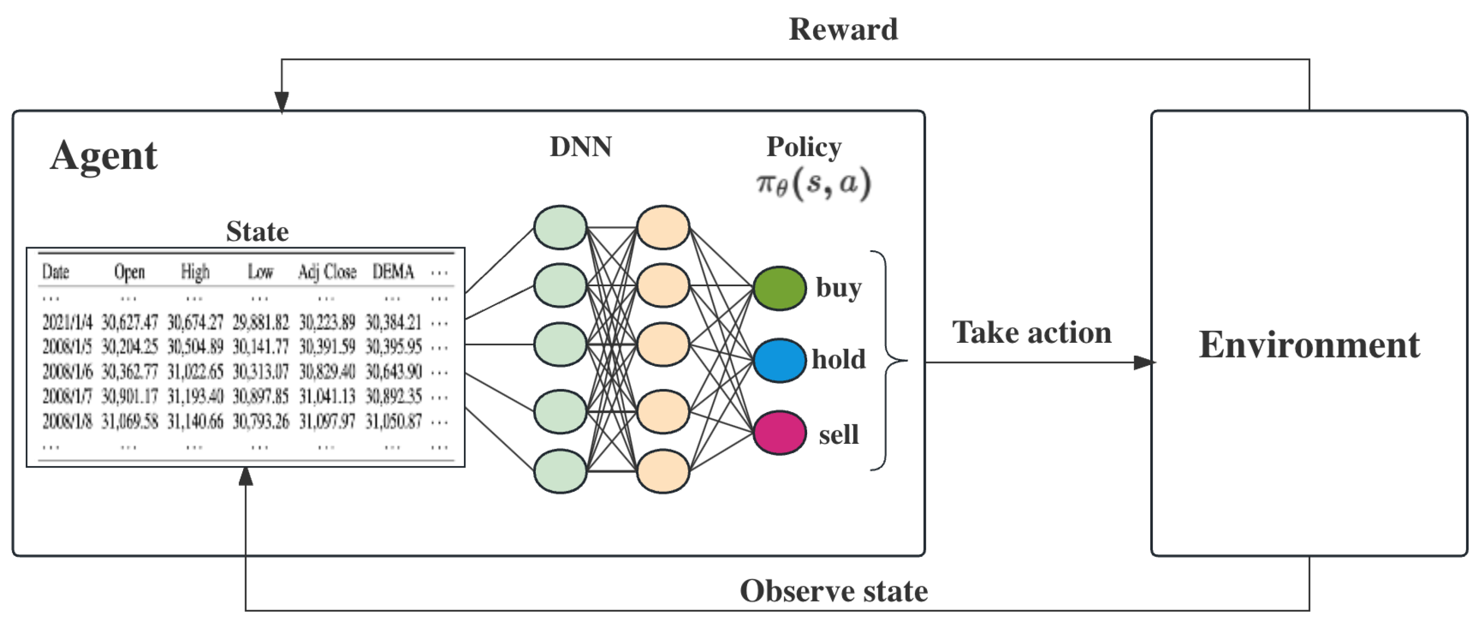
3.1.1. States
3.1.2. Actions
3.1.3. Reward Function
3.2. Methods
3.2.1. Dual Action and Dual Environment Deep Q-Network (DADE-DQN)
3.2.2. Feature Selection Based on Mutual Information
3.2.3. DADE-DQN Training
| Algorithm 1 DADE-DQN algorithm |
|
4. Experiments and Results
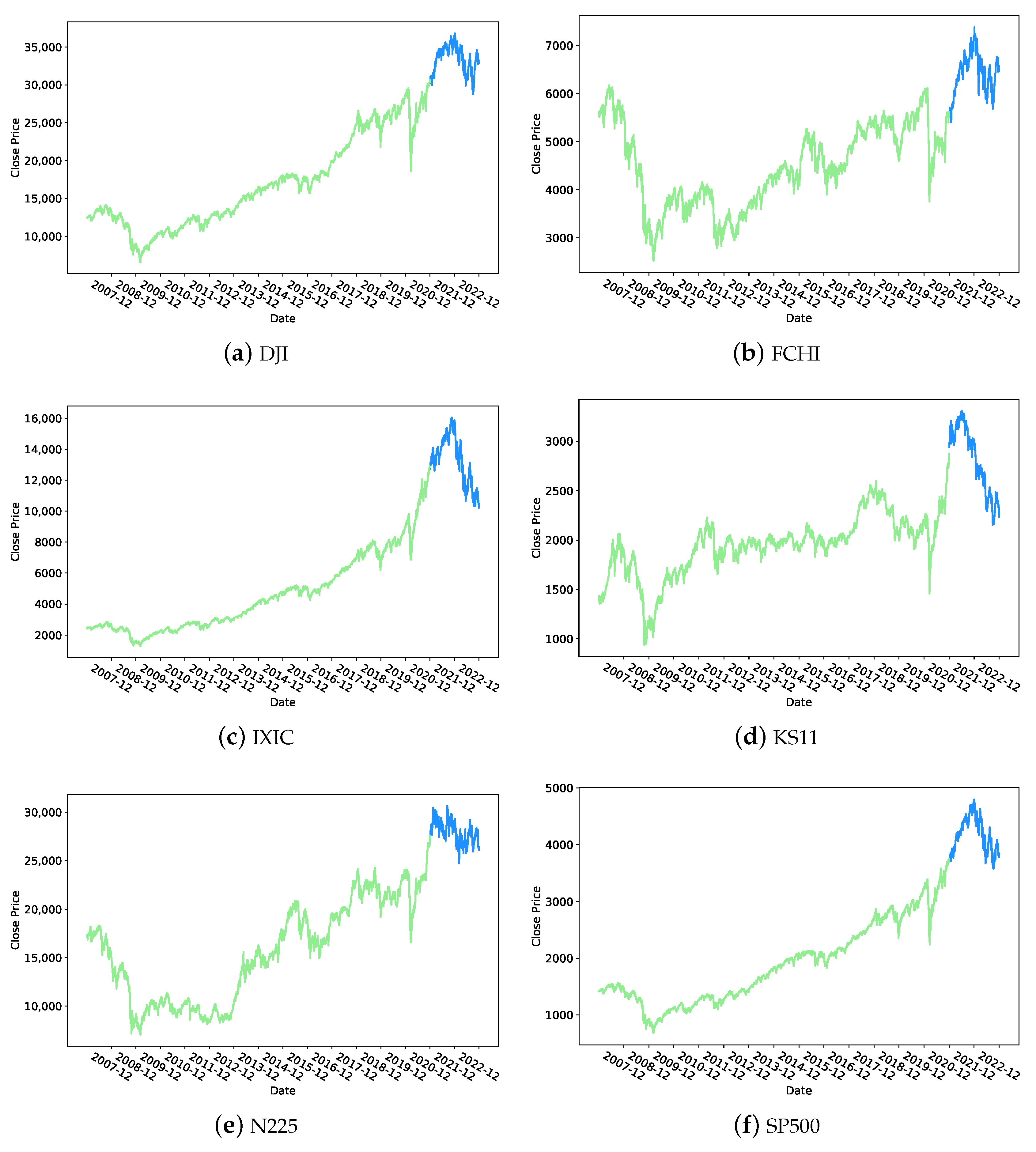
4.1. Datasets
4.2. Feature Selection Results
4.3. Experiment Settings
- Preprocessing: Preprocessing was performed by normalizing each input variable to ensure consistent scaling and prevent gradient explosions. This normalization resulted in a mean of 0 and a standard deviation of 1 for the normalized data.
- Initialization: Xavier initialization was employed to enhance the convergence of the algorithm by setting the initial weights in a manner that maintained a constant variance of gradients across the deep neural network layers.
- Performance metrics: To accurately evaluate the performance of the trading strategies, four performance metrics were selected, namely cumulative return (CR), Sharpe ratio (SR), maximum drawdown (MDD), and annualized return (AR). These metrics provide a comprehensive and objective analysis of the strategy’s benefits and drawbacks in terms of profitability and risk management.
- Baseline methods: To objectively evaluate the advantages and disadvantages of the DADE-DQN algorithm, a comparison was made with traditional methods like buy and hold (B&H), sell and hold (S&H), mean reversion with moving averages (MR), and trend following with moving averages (TF) [60,61,62], as well as DRL methods including TDQN [31], DQN-Vanilla, and DQN-Pattern [34].
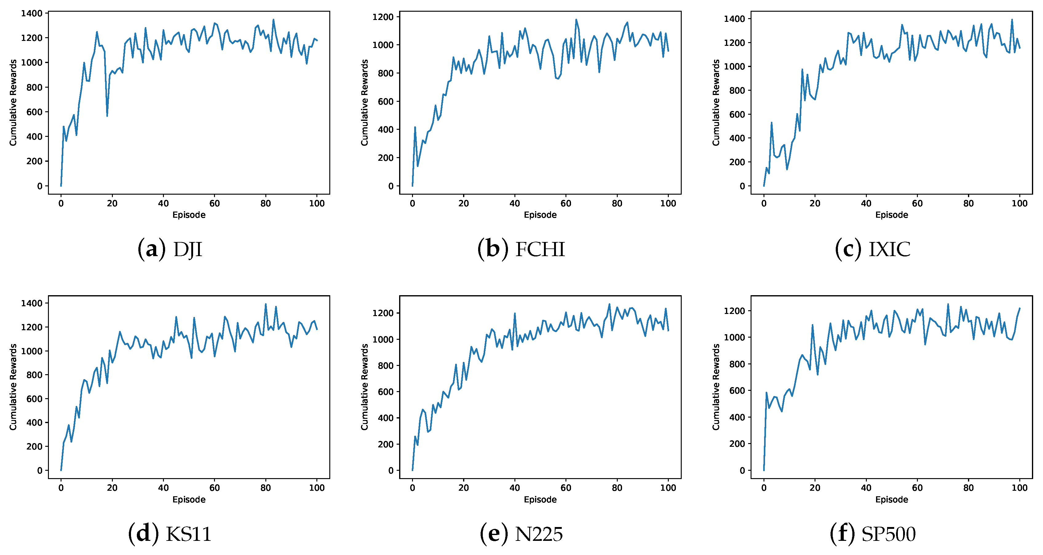
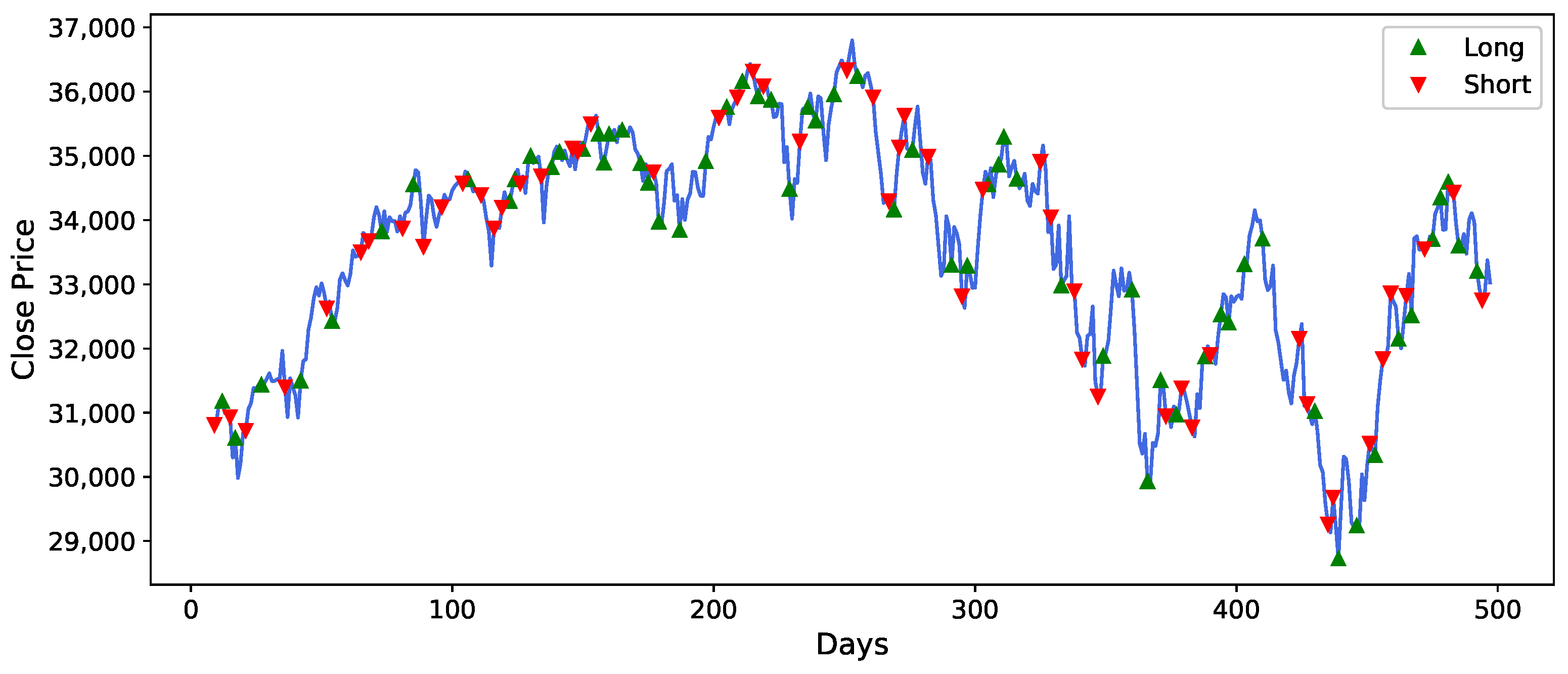
4.4. Experimental Results
5. Discussion
6. Conclusions and Future Work
Author Contributions
Funding
Data Availability Statement
Acknowledgments
Conflicts of Interest
References
- Hamilton, J.D. Time Series Analysis; Princeton University Press: Princeton, NJ, USA, 2020. [Google Scholar]
- Hambly, B.; Xu, R.; Yang, H. Recent Advances in Reinforcement Learning in Finance. Math. Financ. 2021, 33, 435–975. [Google Scholar] [CrossRef]
- Silver, D.; Schrittwieser, J.; Simonyan, K.; Antonoglou, I.; Hassabis, D. Mastering the game of Go without human knowledge. Nature 2017, 550, 354–359. [Google Scholar] [CrossRef] [PubMed]
- Vinyals, O.; Babuschkin, I.; Czarnecki, W.M.; Mathieu, M.; Dudzik, A.; Chung, J.; Choi, D.H.; Powell, R.; Ewalds, T.; Georgiev, P.; et al. Grandmaster level in StarCraft II using multi-agent reinforcement learning. Nature 2019, 575, 350–354. [Google Scholar] [CrossRef] [PubMed]
- Berner, C.; Brockman, G.; Chan, B.; Cheung, V.; Debiak, P.; Dennison, C.; Farhi, D.; Fischer, Q.; Hashme, S.; Hesse, C.; et al. Dota 2 with Large Scale Deep Reinforcement Learning. arXiv 2019, arXiv:1912.06680. [Google Scholar]
- Mnih, V.; Kavukcuoglu, K.; Silver, D.; Graves, A.; Antonoglou, I.; Wierstra, D.; Riedmiller, M. Playing Atari with Deep Reinforcement Learning. Comput. Sci. 2013. [Google Scholar]
- Hasselt, H.V.; Guez, A.; Silver, D. Deep Reinforcement Learning with Double Q-Learning. In Proceedings of the AAAI Conference on Artificial Intelligence, Austin, TX, USA, 25–30 January 2015. [Google Scholar]
- Lipton, Z.C.; Gao, J.; Li, L.; Li, X.; Ahmed, F.; Deng, L. Efficient exploration for dialog policy learning with deep BBQ networks & replay buffer spiking. arXiv 2016, arXiv:1608.05081. [Google Scholar]
- Mossalam, H.; Assael, Y.M.; Roijers, D.M.; Whiteson, S. Multi-objective deep reinforcement learning. arXiv 2016, arXiv:1610.02707. [Google Scholar]
- Mahajan, A.; Tulabandhula, T. Symmetry Learning for Function Approximation in Reinforcement Learning. arXiv 2017, arXiv:1706.02999. [Google Scholar]
- Taitler, A.; Shimkin, N. Learning control for air hockey striking using deep reinforcement learning. In Proceedings of the 2017 International Conference on Control, Artificial Intelligence, Robotics & Optimization (ICCAIRO), Prague, Czech Republic, 20–22 May 2017; pp. 22–27. [Google Scholar]
- Levine, N.; Zahavy, T.; Mankowitz, D.J.; Tamar, A.; Mannor, S. Shallow updates for deep reinforcement learning. In Proceedings of the Advances in Neural Information Processing Systems, Long Beach, CA, USA, 4–9 December 2017; Volume 30. [Google Scholar]
- Leibfried, F.; Grau-Moya, J.; Bou-Ammar, H. An Information-Theoretic Optimality Principle for Deep Reinforcement Learning. arXiv 2017, arXiv:1708.01867. [Google Scholar]
- Anschel, O.; Baram, N.; Shimkin, N. Averaged-dqn: Variance reduction and stabilization for deep reinforcement learning. In Proceedings of the International Conference on Machine Learning, Sydney, Australia, 6–11 August 2017; pp. 176–185. [Google Scholar]
- Hester, T.; Vecerík, M.; Pietquin, O.; Lanctot, M.; Schaul, T.; Piot, B.; Sendonaris, A.; Dulac-Arnold, G.; Osband, I.; Agapiou, J.P.; et al. Learning from Demonstrations for Real World Reinforcement Learning. arXiv 2017, arXiv:1704.03732. [Google Scholar]
- Schaul, T.; Quan, J.; Antonoglou, I.; Silver, D. Prioritized experience replay. arXiv 2015, arXiv:1511.05952. [Google Scholar]
- Sorokin, I.; Seleznev, A.; Pavlov, M.; Fedorov, A.; Ignateva, A. Deep Attention Recurrent Q-Network. arXiv 2015, arXiv:1512.01693. [Google Scholar]
- Hausknecht, M.; Stone, P. Deep recurrent q-learning for partially observable mdps. In Proceedings of the 2015 AAAI Fall Symposium Series, Arlington, VA, USA, 12–14 November 2015. [Google Scholar]
- Wang, Z.; Schaul, T.; Hessel, M.; Hasselt, H.; Lanctot, M.; Freitas, N. Dueling network architectures for deep reinforcement learning. In Proceedings of the International Conference on Machine Learning, New York, NY, USA, 20–22 June 2016; pp. 1995–2003. [Google Scholar]
- Mosavi, A.; Ghamisi, P.; Faghan, Y.; Duan, P.; Band, S. Comprehensive Review of Deep Reinforcement Learning Methods and Applications in Economics; Social Science Electronic Publishing: Rochester, NY, USA, 2020. [Google Scholar]
- Thakkar, A.; Chaudhari, K. A Comprehensive Survey on Deep Neural Networks for Stock Market: The Need, Challenges, and Future Directions. Expert Syst. Appl. 2021, 177, 114800. [Google Scholar] [CrossRef]
- Gao, X. Deep reinforcement learning for time series: Playing idealized trading games. arXiv 2018, arXiv:1803.03916. [Google Scholar]
- Huang, C.Y. Financial Trading as a Game: A Deep Reinforcement Learning Approach. arXiv 2018, arXiv:1807.02787. [Google Scholar]
- Chen, L.; Gao, Q. Application of Deep Reinforcement Learning on Automated Stock Trading. In Proceedings of the 2019 IEEE 10th International Conference on Software Engineering and Service Science (ICSESS), Beijing, China, 18–20 October 2019; pp. 29–33. [Google Scholar]
- Jeong, G.H.; Kim, H.Y. Improving financial trading decisions using deep Q-learning: Predicting the number of shares, action strategies, and transfer learning. Expert Syst. Appl. 2019, 117, 125–138. [Google Scholar] [CrossRef]
- Li, Y.; Nee, M.; Chang, V. An Empirical Research on the Investment Strategy of Stock Market based on Deep Reinforcement Learning model. In Proceedings of the 4th International Conference on Complexity, Future Information Systems and Risk, Crete, Greece, 2–4 May 2019. [Google Scholar]
- Chakole, J.; Kurhekar, M. Trend following deep Q-Learning strategy for stock trading. Expert Syst. 2020, 37, e12514. [Google Scholar] [CrossRef]
- Dang, Q.V. Reinforcement learning in stock trading. In Advanced Computational Methods for Knowledge Engineering, Proceedings of the 6th International Conference on Computer Science, Applied Mathematics and Applications, ICCSAMA 2019, Hanoi, Vietnam, 19–20 December 2019; Springer International Publishing: Cham, Switzerland, 2019; pp. 311–322. [Google Scholar]
- Ma, C.; Zhang, J.; Liu, J.; Ji, L.; Gao, F. A Parallel Multi-module Deep Reinforcement Learning Algorithm for Stock Trading. Neurocomputing 2021, 449, 290–302. [Google Scholar] [CrossRef]
- Shi, Y.; Li, W.; Zhu, L.; Guo, K.; Cambria, E. Stock trading rule discovery with double deep Q-network. Appl. Soft Comput. 2021, 107, 107320. [Google Scholar] [CrossRef]
- Théate, T.; Ernst, D. An application of deep reinforcement learning to algorithmic trading. Expert Syst. Appl. 2021, 173, 114632. [Google Scholar] [CrossRef]
- Bajpai, S. Application of deep reinforcement learning for Indian stock trading automation. arXiv 2021, arXiv:2106.16088. [Google Scholar]
- Li, Y.; Liu, P.; Wang, Z. Stock Trading Strategies Based on Deep Reinforcement Learning. Sci. Program. 2022, 2022, 4698656. [Google Scholar] [CrossRef]
- Taghian, M.; Asadi, A.; Safabakhsh, R. Learning financial asset-specific trading rules via deep reinforcement learning. Expert Syst. Appl. 2022, 195, 116523. [Google Scholar] [CrossRef]
- Liu, P.; Zhang, Y.; Bao, F.; Yao, X.; Zhang, C. Multi-type data fusion framework based on deep reinforcement learning for algorithmic trading. Appl. Intell. 2023, 53, 1683–1706. [Google Scholar] [CrossRef]
- Tran, M.; Pham-Hi, D.; Bui, M. Optimizing Automated Trading Systems with Deep Reinforcement Learning. Algorithms 2023, 16, 23. [Google Scholar] [CrossRef]
- Huang, Y.; Cui, K.; Song, Y.; Chen, Z. A Multi-Scaling Reinforcement Learning Trading System Based on Multi-Scaling Convolutional Neural Networks. Mathematics 2023, 11, 2467. [Google Scholar] [CrossRef]
- Ye, Z.J.; Schuller, B.W. Human-Aligned Trading by Imitative Multi-Loss Reinforcement Learning. Expert Syst. Appl. 2023, 234, 120939. [Google Scholar] [CrossRef]
- Moody, J.; Saffell, M. Learning to trade via direct reinforcement. IEEE Trans. Neural Netw. 2001, 12, 875–889. [Google Scholar] [CrossRef]
- Lele, S.; Gangar, K.; Daftary, H.; Dharkar, D. Stock market trading agent using on-policy reinforcement learning algorithms. Soc. Sci. Electron. Publ. 2020. [Google Scholar] [CrossRef]
- Liu, F.; Li, Y.; Li, B.; Li, J.; Xie, H. Bitcoin transaction strategy construction based on deep reinforcement learning. Appl. Soft Comput. 2021, 113, 107952. [Google Scholar] [CrossRef]
- Wang, Z.; Lu, W.; Zhang, K.; Li, T.; Zhao, Z. A parallel-network continuous quantitative trading model with GARCH and PPO. arXiv 2021, arXiv:2105.03625. [Google Scholar]
- Mahayana, D.; Shan, E.; Fadhl’Abbas, M. Deep Reinforcement Learning to Automate Cryptocurrency Trading. In Proceedings of the 2022 12th International Conference on System Engineering and Technology (ICSET), Bandung, Indonesia, 3–4 October 2022; pp. 36–41. [Google Scholar]
- Xiao, X. Quantitative Investment Decision Model Based on PPO Algorithm. Highlights Sci. Eng. Technol. 2023, 34, 16–24. [Google Scholar] [CrossRef]
- Ponomarev, E.; Oseledets, I.V.; Cichocki, A. Using reinforcement learning in the algorithmic trading problem. J. Commun. Technol. Electron. 2019, 64, 1450–1457. [Google Scholar] [CrossRef]
- Liu, X.Y.; Yang, H.; Chen, Q.; Zhang, R.; Yang, L.; Xiao, B.; Wang, C.D. FinRL: A deep reinforcement learning library for automated stock trading in quantitative finance. arXiv 2020, arXiv:2011.09607. [Google Scholar]
- Liu, Y.; Liu, Q.; Zhao, H.; Pan, Z.; Liu, C. Adaptive quantitative trading: An imitative deep reinforcement learning approach. In Proceedings of the AAAI Conference on Artificial Intelligence, New York, NY, USA, 7–12 February 2020; pp. 2128–2135. [Google Scholar]
- Lima Paiva, F.C.; Felizardo, L.K.; Bianchi, R.A.d.C.; Costa, A.H.R. Intelligent trading systems: A sentiment-aware reinforcement learning approach. In Proceedings of the Second ACM International Conference on AI in Finance, Virtual, 3–5 November 2021; pp. 1–9. [Google Scholar]
- Vishal, M.; Satija, Y.; Babu, B.S. Trading Agent for the Indian Stock Market Scenario Using Actor-Critic Based Reinforcement Learning. In Proceedings of the 2021 IEEE International Conference on Computation System and Information Technology for Sustainable Solutions (CSITSS), Bangalore, India, 16–18 December 2021; pp. 1–5. [Google Scholar]
- Ge, J.; Qin, Y.; Li, Y.; Huang, Y.; Hu, H. Single stock trading with deep reinforcement learning: A comparative study. In Proceedings of the 2022 14th International Conference on Machine Learning and Computing (ICMLC), Guangzhou, China, 18–21 February 2022; pp. 34–43. [Google Scholar]
- Nesselroade, K.P., Jr.; Grimm, L.G. Statistical Applications for the Behavioral and Social Sciences; John Wiley & Sons: Hoboken, NJ, USA, 2018. [Google Scholar]
- Cai, J.; Xu, K.; Zhu, Y.; Hu, F.; Li, L. Prediction and analysis of net ecosystem carbon exchange based on gradient boosting regression and random forest. Appl. Energy 2020, 262, 114566. [Google Scholar] [CrossRef]
- Li, G.; Zhang, A.; Zhang, Q.; Wu, D.; Zhan, C. Pearson Correlation Coefficient-Based Performance Enhancement of Broad Learning System for Stock Price Prediction. IEEE Trans. Circuits Syst. II Express Briefs 2022, 69, 2413–2417. [Google Scholar] [CrossRef]
- Guo, X.; Zhang, H.; Tian, T. Development of stock correlation networks using mutual information and financial big data. PLoS ONE 2018, 13, e195941. [Google Scholar] [CrossRef]
- Kong, A.; Azencott, R.; Zhu, H.; Li, X. Pattern Recognition in Microtrading Behaviors Preceding Stock Price Jumps: A Study Based on Mutual Information for Multivariate Time Series. Comput. Econ. 2023, 1–29. [Google Scholar] [CrossRef]
- Sutton, R.; Barto, A. Reinforcement Learning: An Introduction; MIT Press: Cambridge, MA, USA, 1998. [Google Scholar]
- Yue, H.; Liu, J.; Zhang, Q. Applications of Markov Decision Process Model and Deep Learning in Quantitative Portfolio Management during the COVID-19 Pandemic. Systems 2022, 10, 146. [Google Scholar] [CrossRef]
- Yang, Z.; Yang, D.; Dyer, C.; He, X.; Smola, A.; Hovy, E. Hierarchical attention networks for document classification. In Proceedings of the 2016 Conference of the North American Chapter of the Association for Computational Linguistics: Human Language Technologies, San Diego, CA, USA, 12 June–17 June 2016; pp. 1480–1489. [Google Scholar]
- Hochreiter, S.; Schmidhuber, J. Long short-term memory. Neural Comput. 1997, 9, 1735–1780. [Google Scholar] [CrossRef]
- Chan, E. Algorithmic Trading: Winning Strategies and Their Rationale; John Wiley & Sons: Hoboken, NJ, USA, 2013; Volume 625. [Google Scholar]
- Narang, R.K. Inside the Black Box: A Simple Guide to Quantitative and High Frequency Trading; John Wiley & Sons: Hoboken, NJ, USA, 2013; Volume 846. [Google Scholar]
- Chan, E.P. Quantitative Trading: How to Build Your Own Algorithmic Trading Business; John Wiley & Sons: Hoboken, NJ, USA, 2021. [Google Scholar]


| Article | Data Set | State Space | Action Space | Reward | Method | Performance |
|---|---|---|---|---|---|---|
| 1-7 [22] (2018) | Artificial time series | prices | cash, buy, hold | return | DQN + CNN, LSTM, GRU, MLP | mean profit |
| 1-7 [23] (2018) | foreign exchange | OHLCV, position | hold, buy, sell | log return | DRQN + LSTM | profit, return, ShR, SoR, WR, MDD etc. |
| 1-7 [24] (2019) | SPY (S&P500 ETF) | adjusted closes | buy, sell, hold | return | DQN, DRQN + RNN | AmR |
| 1-7 [25] (2019) | S&P500, KOSPI, HSI, EuroStoxx50 | 200-days prices | buy, sell, hold | return rate | DQN + MLP | profit, correlation |
| 1-7 [26] (2019) | 10 U.S. stocks | prices, volumes | buy, sell, hold | none | Dueling DQN, DDQN, DQN + MLP, CNN | profit |
| 1-7 [27] (2020) | 2 U.S indices, 2 Indian indices | closing prices | long, short, neutral | return | DQN | returns, MDD, ShR, Skewness, AR, Kurtosis etc. |
| 1-7 [28] (2020) | prices | buy, sell, hold | profit | Dueling DQN, DQN, DDQN + CNN | profit | |
| 1-7 [29] (2021) | Chinese stocks | OHLCV, technical indicators | buy, sell, hold | return | DDQN + DNN, LSTM | returns, ShR |
| 1-7 [30] (2021) | Chinese stocks, U.S. stocks | OHLCV, action | long/buy, short/sell | return | DDQN + CNN | accuracy, profit, returns, MDD |
| 1-7 [31] (2021) | 30 stocks | OHLCV, position | buy, sell | return | DDQN + CNN | profit, ShR, MDD, MDDD, AR, SoR etc. |
| 1-7 [32] (2021) | Indian market | prices, volume | buy, sell, hold | none | DQN, DDQN, Dueling DDQN + CNN | profit |
| 1-7 [33] (2022) | S&P 500, Chinese stocks | technical indicators, candlestick charts | long, short, neural | ShR + PR | Dueling DQN, DDQN + CNN, BiLSTM | AR, ShR, MDD |
| 1-7 [34] (2022) | AAPL, GOOGL, KSS, BTC/USD | OHLC | buy, sell, hold | customized | SARSA, DQN + MLP, CNN, GRU | AR, TR, VaR, ShR, MDD |
| 1-7 [35] (2023) | Chinese stock, S&P 500 stocks | OHLCV, technical indicators, candlestick charts | buy, sell, hold | profit | Dueling DQN, DDQN + CNN, LSTM, BiLSTM | profit, AR, ShR, MDD, MDDD |
| 1-7 [36] (2023) | BTC-USDT | OHLC | buy, sell, hold | ShR | Dueling DQN, DDQN + CNN | average return |
| 1-7 [37] (2023) | Dow Jones, NASDAQ, General Electric, AAPLE | OHLCV | buy, sell, hold | ShR | SARSA + CNN | profit, AR, ShR |
| 1-7 [38] (2023) | 10 stocks (AAPL etc.) | close price | buy, sell, hold | profit | Mult-step DQN + LSTM | return, CR |
| 1-7 Our | Six stock indices | OHLC, technical indicators | buy, sell, hold | ShR | DDQN + LSTM + attention mechanisms | CR, AR, ShR, MDD |
| Categories | Feature Name | Description |
|---|---|---|
| Overlapping Indicators | DEMA | Double Exponential Moving Average |
| SMA_3 | Simple Moving Average (3 days) | |
| SMA_5 | Simple Moving Average (5 days) | |
| SMA_10 | Simple Moving Average (10 days) | |
| BBANDS_UP | Bollinger BandsDEMA (UP) | |
| BBANDS_MIDDLE | Bollinger BandsDEMA (MIDDLE) | |
| BBANDS_LOW | Bollinger BandsDEMA (LOW) | |
| EMA | Exponential Moving Average | |
| HT_TRENDLINE | Hilbert Transform— Instantaneous Trendline | |
| KAMA | Kaufman Adaptive Moving Average | |
| MA | All Moving Average | |
| SAR | Parabolic SAR | |
| Momentum Indicators | ADX | Average Directional Movement Index |
| AROONOSC | Aroon Oscillator | |
| RSI | Relative Strength Index | |
| MFI | Money Flow Index | |
| MOM | Momentum | |
| WILLR | Williams’ %R | |
| TRIX | 1-day Rate-Of-Change (ROC) of a Triple Smooth EMA | |
| PPO | Percentage Price Oscillator | |
| BOP | Balance Of Power | |
| DIF | Moving Average Convergence/Divergence | |
| DEM | Moving Average Convergence/Divergence | |
| HISTOGRAM | Moving Average Convergence/Divergence | |
| ROC | Rate of change: | |
| ADXR | Average Directional Movement Index Rating | |
| APO | Absolute Price Oscillator | |
| AROON_UP | Strength of the upward trend | |
| CCI | Commodity Channel Index | |
| PLUS_DI | Plus Directional Indicator | |
| CMO | Chande Momentum Oscillator | |
| ROCP | Rate of change Percentage: | |
| RR | Daily simple rate of return | |
| LOG_RR | Daily log returns | |
| Volume Indicators | AD | Chaikin A/D Line |
| ADOSC | Chaikin A/D Oscillator | |
| OBV | On Balance Volume | |
| Volatility Indicators | NATR | Normalized Average True Range |
| ATR | Average True Range | |
| TRANGE | True Range | |
| Price Change Indicators | AVGPRICE | Average Price |
| MEDPRICE | Median Price | |
| TYPPRICE | Typical Price | |
| WCLPRICE | Weighted Close Price | |
| Periodic Indicators | HT_DCPERIOD | Hilbert Transform—Dominant Cycle Period |
| HT_DCPHASE | Hilbert Transform—Dominant Cycle Phase | |
| INPHASE | Hilbert Transform—Phasor Components | |
| QUADRATURE | Hilbert Transform—Phasor Components | |
| SINE | Hilbert Transform—SineWave | |
| LEADSINE | Hilbert Transform—SineWave | |
| HT_TRENDMODE | Hilbert Transform—Trend vs. Cycle Mode | |
| Statistical Indicators | BETA | Beta |
| TSF | Time Series Forecast | |
| Raw Data | Open | Open price |
| Low | Low price | |
| High | High price | |
| Volume | Trading volume |
| Feature | DJI | FCHI | IXIC | KS11 | N225 | SP500 |
|---|---|---|---|---|---|---|
| DEMA | 4.1177 | 3.3413 | 4.3570 | 3.2748 | 3.7140 | 4.2179 |
| SMA_3 | 3.7271 | 2.9425 | 3.9640 | 2.8457 | 3.2789 | 3.8332 |
| SMA_5 | 3.3791 | 2.5757 | 3.6082 | 2.4649 | 2.9325 | 3.4812 |
| SMA_10 | 3.0716 | 2.2392 | 3.3372 | 2.0869 | 2.5346 | 3.2159 |
| BBANDS_UP | 3.4327 | 2.6122 | 3.6738 | 2.5206 | 2.9584 | 3.5264 |
| BBANDS_MIDDLE | 3.3791 | 2.5757 | 3.6082 | 2.4649 | 2.9325 | 3.4812 |
| BBANDS_LOW | 3.3193 | 2.6309 | 3.5638 | 2.5015 | 2.9366 | 3.4449 |
| EMA | 3.6016 | 2.8031 | 3.8492 | 2.6916 | 3.1308 | 3.7237 |
| HT_TRENDLINE | 2.8111 | 1.8744 | 3.0767 | 1.6562 | 2.1876 | 2.9604 |
| KAMA | 2.8897 | 1.9904 | 3.1711 | 1.8767 | 2.3706 | 2.9943 |
| MA | 2.8822 | 1.9745 | 3.1665 | 1.7855 | 2.2974 | 2.9875 |
| SAR | 0.7567 | 0.0632 | 0.5591 | 0.4079 | 0.5781 | 0.7737 |
| ADX | 0.3911 | 0.1834 | 0.3769 | 0.2700 | 0.2881 | 0.3232 |
| AROONOSC | 0.3703 | 0.2319 | 0.3567 | 0.1856 | 0.3223 | 0.3511 |
| RSI | 0.3073 | 0.2390 | 0.2215 | 0.2921 | 0.2919 | 0.2406 |
| MFI | 0.2990 | 0.1842 | 0.4474 | 0.2264 | 0.3132 | 0.4289 |
| MOM | 0.2128 | 0.1223 | 0.3048 | 0.1262 | 0.1692 | 0.2085 |
| WILLR | 0.0960 | 0.1021 | 0.0693 | 0.0739 | 0.1003 | 0.0955 |
| TRIX | 0.9735 | 0.6552 | 1.0965 | 0.7253 | 0.8499 | 1.0828 |
| PPO | 0.4377 | 0.2552 | 0.4563 | 0.3123 | 0.3044 | 0.4465 |
| DIF | 0.6538 | 0.3573 | 0.8089 | 0.4175 | 0.4798 | 0.6663 |
| DEM | 0.6997 | 0.3663 | 0.8898 | 0.3949 | 0.5235 | 0.7089 |
| HISTOGRAM | 0.3269 | 0.1597 | 0.3312 | 0.1912 | 0.2279 | 0.2925 |
| ROC | 0.1774 | 0.1460 | 0.1774 | 0.1638 | 0.1606 | 0.1793 |
| ADXR | 0.5443 | 0.2849 | 0.5293 | 0.3817 | 0.4301 | 0.4915 |
| APO | 0.5044 | 0.2010 | 0.6402 | 0.2815 | 0.3118 | 0.5028 |
| AROON_UP | 0.0198 | 0.0257 | 0.0000 | 0.0315 | 0.0000 | 0.0000 |
| CCI | 0.0913 | 0.0527 | 0.0536 | 0.0708 | 0.0888 | 0.0466 |
| PLUS_DI | 0.2150 | 0.1669 | 0.1908 | 0.1680 | 0.1969 | 0.1760 |
| CMO | 0.3073 | 0.2390 | 0.2215 | 0.2921 | 0.2919 | 0.2406 |
| ROCP | 0.1774 | 0.1460 | 0.1774 | 0.1638 | 0.1606 | 0.1793 |
| RR | 0.0796 | 0.0450 | 0.0654 | 0.0617 | 0.0242 | 0.0942 |
| LOG RR | 0.0790 | 0.0454 | 0.0650 | 0.0617 | 0.0240 | 0.0944 |
| AD | 2.8611 | 1.8524 | 3.3141 | 1.7776 | 1.7214 | 3.0831 |
| ADOSC | 0.3156 | 0.1419 | 0.1676 | 0.1312 | 0.1273 | 0.1702 |
| OBV | 2.5657 | 1.3280 | 3.0720 | 1.4878 | 2.1969 | 2.7141 |
| NATR | 1.0036 | 0.7114 | 1.0310 | 0.6404 | 0.5802 | 1.0850 |
| ATR | 0.9430 | 0.4994 | 1.2376 | 0.4829 | 0.6761 | 0.9683 |
| TRANGE | 0.1966 | 0.0502 | 0.2877 | 0.1059 | 0.1375 | 0.1681 |
| AVGPRICE | 4.2120 | 3.5395 | 4.5136 | 3.4856 | 4.0977 | 4.3229 |
| MEDPRICE | 4.1514 | 3.4655 | 4.4266 | 3.4079 | 4.0328 | 4.2623 |
| TYPPRICE | 4.5448 | 3.8758 | 4.8251 | 3.8178 | 4.4584 | 4.6562 |
| WCLPRICE | 4.8117 | 4.1710 | 5.0773 | 4.1032 | 4.7400 | 4.9200 |
| HT_DCPERIOD | 0.3719 | 0.2053 | 0.2927 | 0.1784 | 0.2862 | 0.3396 |
| HT_DCPHASE | 0.1776 | 0.0672 | 0.1850 | 0.1042 | 0.1497 | 0.1745 |
| INPHASE | 0.1469 | 0.0158 | 0.2421 | 0.0666 | 0.1238 | 0.1734 |
| QUADRATURE | 0.1121 | 0.0049 | 0.1233 | 0.0300 | 0.0400 | 0.0777 |
| SINE | 0.1040 | 0.0198 | 0.0972 | 0.0390 | 0.1012 | 0.1004 |
| LEADSINE | 0.1470 | 0.0659 | 0.1672 | 0.0839 | 0.1157 | 0.1302 |
| HT_TRENDMODE | 0.0667 | 0.0400 | 0.0724 | 0.0275 | 0.0565 | 0.0610 |
| BETA | 0.0937 | 0.0701 | 0.0871 | 0.0761 | 0.0917 | 0.0834 |
| TSF | 3.2989 | 2.4815 | 3.5202 | 2.3681 | 2.8195 | 3.4074 |
| Open | 3.4958 | 2.8795 | 3.8893 | 2.8079 | 3.3896 | 3.6429 |
| Low | 4.1668 | 3.5306 | 4.4530 | 3.4674 | 4.0848 | 4.2808 |
| High | 4.2085 | 3.5045 | 4.5037 | 3.4317 | 4.0687 | 4.3466 |
| Volume | 0.7044 | 0.2008 | 0.3621 | 0.1448 | 0.4166 | 0.3471 |
| Feature | DJI | FCHI | IXIC | KS11 | N225 | SP500 |
|---|---|---|---|---|---|---|
| DEMA | 4.1177 | 3.3413 | 4.3570 | 3.2748 | 3.7140 | 4.2179 |
| SMA_3 | 3.7271 | 2.9425 | 3.9640 | 2.8457 | 3.2789 | 3.8332 |
| SMA_5 | 3.3791 | 2.5757 | 3.6082 | 2.4649 | 2.9325 | 3.4812 |
| SMA_10 | 3.0716 | 2.2392 | 3.3372 | 2.0869 | 2.5346 | 3.2159 |
| BBANDS_UP | 3.4327 | 2.6122 | 3.6738 | 2.5206 | 2.9584 | 3.5264 |
| BBANDS_MIDDLE | 3.3791 | 2.5757 | 3.6082 | 2.4649 | 2.9325 | 3.4812 |
| BBANDS_LOW | 3.3193 | 2.6309 | 3.5638 | 2.5015 | 2.9366 | 3.4449 |
| EMA | 3.6016 | 2.8031 | 3.8492 | 2.6916 | 3.1308 | 3.7237 |
| HT_TRENDLINE | 2.8111 | 1.8744 | 3.0767 | 1.6562 | 2.1876 | 2.9604 |
| KAMA | 2.8897 | 1.9904 | 3.1711 | 1.8767 | 2.3706 | 2.9943 |
| MA | 2.8822 | 1.9745 | 3.1665 | 1.7855 | 2.2974 | 2.9875 |
| TRIX | 0.9735 | 0.6552 | 1.0965 | 0.7253 | 0.8499 | 1.0828 |
| AD | 2.8611 | 1.8524 | 3.3141 | 1.7776 | 1.7214 | 3.0831 |
| OBV | 2.5657 | 1.3280 | 3.0720 | 1.4878 | 2.1969 | 2.7141 |
| NATR | 1.0036 | 0.7114 | 1.0310 | 0.6404 | 0.5802 | 1.0850 |
| AVGPRICE | 4.2120 | 3.5395 | 4.5136 | 3.4856 | 4.0977 | 4.3229 |
| MEDPRICE | 4.1514 | 3.4655 | 4.4266 | 3.4079 | 4.0328 | 4.2623 |
| TYPPRICE | 4.5448 | 3.8758 | 4.8251 | 3.8178 | 4.4584 | 4.6562 |
| WCLPRICE | 4.8117 | 4.1710 | 5.0773 | 4.1032 | 4.7400 | 4.9200 |
| TSF | 3.2989 | 2.4815 | 3.5202 | 2.3681 | 2.8195 | 3.4074 |
| Open | 3.4958 | 2.8795 | 3.8893 | 2.8079 | 3.3896 | 3.6429 |
| Low | 4.1668 | 3.5306 | 4.4530 | 3.4674 | 4.0848 | 4.2808 |
| High | 4.2085 | 3.5045 | 4.5037 | 3.4317 | 4.0687 | 4.3466 |
| Metrics | n = 5 | n = 10 | n = 15 | n = 20 |
|---|---|---|---|---|
| Cumulative return (%) | 14.11 | 26.17 | 15.01 | 16.91 |
| Annualized return (%) | 11.08 | 18.24 | 11.91 | 13.34 |
| Sharpe ratio | 0.54 | 0.93 | 0.56 | 0.61 |
| Maximum drawdown (%) | 13.03 | 11.52 | 18.26 | 14.75 |
| Hyperparameter | Value | Hyperparameter | Value |
|---|---|---|---|
| Input size | 24 | Window length (n) | 10 |
| Number of neurons in hidden layer | 64 | Number of LSTM layer | 1 |
| Output size | 3 | Attention weight | 0.1 |
| Activation function | Tanh | Learning rate () | 0.003 |
| Discount factor () | 0.9 | -greedy | 0.9 |
| Number of steps to update the target Q network parameters | 10 | Replay memory size | 1000 |
| Optimizer is Adam with L2Factor | 0.000001 | Episode | 100 |
| Initial capital | USD 500,000 | Trading cost | 0.001 |
| Assets | Metrics | B&H | S&H | MR | TF | TDQN | DQN-Pattern | DQN-Vanilla | DADE-DQN |
|---|---|---|---|---|---|---|---|---|---|
| DJI | CR[%] | 8.10 | −8.30 | −0.28 | −15.90 | −7.97 | 5.31 | 20.47 | 26.17 |
| AR[%] | 7.85 | −3.98 | 1.42 | −11.86 | −2.96 | 5.65 | 14.99 | 18.24 | |
| SR | 0.33 | −0.14 | 0.06 | −0.53 | −0.18 | 0.24 | 0.66 | 0.93 | |
| MDD[%] | 21.70 | 21.27 | 18.36 | 27.09 | 33.00 | 21.94 | 17.21 | 11.52 | |
| FCHI | CR[%] | 17.10 | −17.34 | −20.00 | 10.05 | 15.08 | −13.26 | 16.22 | 43.46 |
| AR[%] | 14.70 | −10.09 | −15.26 | 9.54 | 8.40 | −8.54 | 13.38 | 28.42 | |
| SR | 0.53 | −0.26 | −0.55 | 0.38 | 0.48 | −0.34 | 0.50 | 1.18 | |
| MDD[%] | 22.42 | 32.93 | 25.14 | 23.63 | 28.05 | 30.83 | 22.42 | 20.70 | |
| IXIC | CR[%] | −17.50 | 17.30 | 12.03 | -29.46 | -33.00 | -18.43 | 24.10 | 49.15 |
| AR[%] | −9.94 | 16.63 | 12.65 | −23.51 | −18.75 | −10.12 | 18.29 | 32.22 | |
| SR | −0.26 | 0.45 | 0.36 | −0.65 | −0.68 | −0.26 | 0.62 | 0.99 | |
| MDD[%] | 35.40 | 25.48 | 21.64 | 38.13 | 38.63 | 36.40 | 25.24 | 16.35 | |
| KS11 | CR[%] | −24.47 | 24.27 | −3.87 | 1.06 | −27.31 | −25.03 | 23.11 | 79.43 |
| AR[%] | −20.40 | 18.04 | −1.19 | 2.62 | −15.93 | −19.92 | 16.47 | 43.57 | |
| SR | −0.78 | 0.88 | −0.05 | 0.11 | −0.89 | −0.77 | 0.81 | 2.21 | |
| MDD[%] | 34.61 | 10.74 | 26.12 | 25.73 | 33.13 | 33.65 | 12.84 | 7.63 | |
| N225 | CR[%] | −6.00 | 5.80 | 9.35 | −22.16 | −24.66 | −4.01 | −5.58 | 24.10 |
| AR[%] | −2.24 | 6.89 | 9.27 | 17.94 | −13.50 | −0.30 | −1.55 | 18.25 | |
| SR | −0.08 | 0.25 | 0.35 | −0.68 | −0.70 | −0.01 | −0.05 | 0.75 | |
| MDD[%] | 18.71 | 13.69 | 15.16 | 25.18 | 31.22 | 19.40 | 19.41 | 16.46 | |
| SP500 | CR[%] | 2.81 | −3.01 | 35.33 | −29.32 | −44.34 | 2.92 | 22.45 | 42.37 |
| AR[%] | 4.89 | 1.82 | 24.59 | −25.19 | −33.06 | 4.78 | 16.72 | 27.51 | |
| SR | 0.17 | 0.05 | 0.96 | −0.92 | −1.45 | 0.17 | 0.64 | 1.11 | |
| MDD[%] | 25.34 | 28.20 | 16.41 | 33.25 | 48.41 | 25.43 | 17.50 | 11.04 |
Disclaimer/Publisher’s Note: The statements, opinions and data contained in all publications are solely those of the individual author(s) and contributor(s) and not of MDPI and/or the editor(s). MDPI and/or the editor(s) disclaim responsibility for any injury to people or property resulting from any ideas, methods, instructions or products referred to in the content. |
© 2023 by the authors. Licensee MDPI, Basel, Switzerland. This article is an open access article distributed under the terms and conditions of the Creative Commons Attribution (CC BY) license (https://creativecommons.org/licenses/by/4.0/).
Share and Cite
Huang, Y.; Lu, X.; Zhou, C.; Song, Y. DADE-DQN: Dual Action and Dual Environment Deep Q-Network for Enhancing Stock Trading Strategy. Mathematics 2023, 11, 3626. https://doi.org/10.3390/math11173626
Huang Y, Lu X, Zhou C, Song Y. DADE-DQN: Dual Action and Dual Environment Deep Q-Network for Enhancing Stock Trading Strategy. Mathematics. 2023; 11(17):3626. https://doi.org/10.3390/math11173626
Chicago/Turabian StyleHuang, Yuling, Xiaoping Lu, Chujin Zhou, and Yunlin Song. 2023. "DADE-DQN: Dual Action and Dual Environment Deep Q-Network for Enhancing Stock Trading Strategy" Mathematics 11, no. 17: 3626. https://doi.org/10.3390/math11173626
APA StyleHuang, Y., Lu, X., Zhou, C., & Song, Y. (2023). DADE-DQN: Dual Action and Dual Environment Deep Q-Network for Enhancing Stock Trading Strategy. Mathematics, 11(17), 3626. https://doi.org/10.3390/math11173626