Flexible-Elliptical Spatial Scan Method

Abstract

The detection of disease clusters in spatial data analysis plays a crucial role in public health, while the circular scan method is widely utilized for this purpose, accurately identifying non-circular (irregular) clusters remains challenging and reduces detection accuracy. To overcome this limitation, various extensions have been proposed to effectively detect arbitrarily shaped clusters. In this paper, we combine the strengths of two well-known methods, the flexible and elliptic scan methods, which are specifically designed for detecting irregularly shaped clusters. We leverage the unique characteristics of these methods to create candidate zones capable of accurately detecting irregularly shaped clusters, along with a modified likelihood ratio test statistic. By inheriting the advantages of the flexible and elliptic methods, our proposed approach represents a practical addition to the existing repertoire of spatial data analysis techniques.

1. Introduction

In public health, surveillance procedures that identify disease clusters play an important role in controlling and preventing disease outbreaks. Numerous methods can be used for detecting clustering and clusters. For detecting spatial autocorrelation, methods such as Moran’s I [1] and Geary’s c [2] are commonly used. These methods quantify a global property over the entire study area and indicate whether response values are more similar than they would be under the null hypothesis and that no spatial autocorrelation is present. Therefore, Moran’s I and Geary’s c are global indices of spatial autocorrelation and can be used in situations such as regression analysis when we want to check whether uncorrelated error assumptions are satisfied or as evidence of clustering across the entire study area. In order to detect local spatial clusters, other methods were proposed, e.g., the cluster evaluation permutation procedure [3], the Besag–Newell method [4], and the circular spatial scan method [5,6] and its related extensions.

The circular spatial scan method [5,6] has gained remarkable popularity for finding local clusters compared to the aforementioned methods due to its computational efficiency and its power to detect disease clusters. This method is characterized by (i) the set of candidate zones to be scanned and (ii) the likelihood ratio test (LRT) statistic for each candidate zone. The capability of the spatial scan method in detecting disease clusters inspired other researchers to propose extensions to improve its accuracy, specifically for detecting non-circular (irregularly shaped) clusters. The circular scan method and its extensions, generally, scan the entire study area and identify the candidate zones that obtain the largest value of an LRT statistic.

There are many different approaches for constructing the set of candidate zones and for computing the LRT statistic. Tango and Takahashi [7,8] proposed the flexible scan method, in which non-circular clusters can be detected more accurately by forming a set of candidate zones from a set of connected regions satisfying certain constraints. In the flexible scan method, each connected candidate zone is enclosed within a circle comprised of a pre-specified set of nearest neighbors. Candidate zones coming from the connected regions within the circle may not be large enough (or flexible enough) to include highly irregular and long candidate zones. Additionally, the computational cost of this method becomes increasingly great as the size of the circle is expanded, which may preclude more arbitrarily shaped candidate zones from being considered [7]. The flexible scan method has recently been used to detect high- and low-risk clusters of COVID-19 incidence in Florida [9], high-risk clusters of La Crosse virus disease in the Appalachian region of the United States [10], and high-risk clusters of thyroid cancer incidence in Fukushima, Japan [11].

Kulldorff et al. [12] proposed the elliptic scan method, which includes elliptical candidate zones along with circular ones. Elliptical candidate zones allow the method to detect non-circular clusters with different shapes and different angles when ellipses rotate around their centers. The elliptic method indeed uses a variety of elliptical shapes and angles to identify irregularly shaped clusters; however, its final results are conditional on the selected shapes. As such, the set of elliptical zones may not have enough versatility to cover non-elliptical clusters. The elliptic scan method has recently been used to identify high-risk clusters of paratuberculosis in sheep and goats in southern Spain [13], high- and low-risk clusters of breast and cervical cancer-related mortality in Brazil, and clusters of high nontuberculous mycobacteria infection risk for persons with cystic fibrosis in United States counties [14].

Another extension of the circular scan method is the minimum spanning tree method proposed by Assunção et al. [15], which attempts to construct candidate zones based on the regions that result in the largest LRT statistic. The minimum spanning tree algorithm may detect abnormal clusters that have a star-like shape because a new region can be added to a current candidate zone regardless of whether the LRT increases or decreases in relation to the current candidate zone. This tendency to detect star-shaped clusters is called the “octopus effect”. Costa et al. [16] extended the minimum spanning tree algorithm by imposing early stopping criteria on the method. Specifically, a new region can only be added to the current candidate zone if it increases the current LRT statistic value. Moreover, in order to avoid the octopus effect, Costa et al. [16] proposed additional stopping criteria, specifically, selecting only the regions that share at least two connections with the current candidate zone. A problem with these methods (and also the elliptic and flexible scan methods) is that adding a low-risk region to an existing zone can increase the LRT of the new zone. Philosophically, it seems unwise to include a low-risk region in a cluster, e.g., a region with low standardized mortality ratio (SMR), where SMR is the ratio of observed to expected cases in a region.

In this study, we propose the flexible–elliptical scan method, which combines the flexible and elliptic scan methods to address their respective limitations and leverage their advantages. Our approach involves modifying the set of candidate zones and the likelihood ratio test statistics. We compare the performance of the proposed flexible–elliptical method with the established elliptic and rflex scan methods for identifying irregularly shaped disease clusters. This evaluation includes benchmark data sets comprising 56 diverse irregularly shaped cluster models, as well as real-world data sets such as the northeastern United States and NTM data. Our findings demonstrate a balanced integration between the flexible and elliptic scan methods in accurately detecting irregularly shaped clusters in disease surveillance. The flexible–elliptical method exhibits better flexibility, inheriting the capabilities of the reflex and elliptic methods, particularly in constructing the set of candidate zones. The proposed method offers a streamlined and straightforward approach, eliminating the need for tuning parameters and providing a more adaptable solution to capture irregular cluster shapes.

The structure of this paper is as follows. In Section 2, we describe the methodology of the circular scan method, the elliptic scan method, and the restricted flexible scan method and then propose a new flexible–elliptical scan method. In Section 3, we benchmark the performance of these scan methods and outline the results using simulated data sets based on the breast cancer mortality of the northeastern United States made available by Kulldorff [6]. In Section 4, we apply these methods to identifying clusters of the northeastern United States data set [17,18]. Additionally, in Section 5, we apply these methods to identifying and comparing clusters of nontuberculous mycobacterial (NTM) cases in Colorado. In Section 6, we draw specific conclusions about the proposed methodology from our study. Finally, in Section 7, we more broadly discuss the strengths and weaknesses of the proposed methodology and comment on future work.

2. Methods

Consider a geographical map (study area) that is partitioned into N regions (e.g., zip codes). Each region is represented by its centroid i, $i=1,\dots ,N$, which is a geographical location inside the region. For each region, we know (i) the population size, $n_i$ and (ii) the number of cases, $Y_i$. Let $\mathbf{Z}$ denote a candidate zone that is formed from the union of one or more (typically connected) regions. Let $\mathcal{Z}$ be the set of candidate zones. Each $\mathbf{Z}\in \mathcal{Z}$ is a potential cluster for which we believe the risk of developing disease inside $\mathbf{Z}$ is higher than the risk of developing disease outside $\mathbf{Z}$. Let p denote the risk of developing disease inside $\mathbf{Z}$. Let q denote the risk of developing disease outside $\mathbf{Z}$. Therefore, under the null hypothesis of no clustering, $p=q$ for all $\mathbf{Z}\in \mathcal{Z}$ (the complete list of notation can be found at the end of the paper before Appendix A). The alternative hypothesis states that there is at least one cluster in the study area, i.e., there is at least one $\mathbf{Z}\in \mathcal{Z}$ such that $p>q$. More formally,

$$H_0:p=q \mathrm{for} \mathrm{all} \mathbf{Z}\in \mathcal{Z}\mathrm{versus}{H}_1:p>q \mathrm{for} \mathrm{some} \mathbf{Z}\in \mathcal{Z}.$$

(1)

In general, the scan methodologies described in this paper are characterized by (i) the set of candidate zones to be scanned, $\mathcal{Z}$, and (ii) the LRT statistic, $\lambda$. We will use different subscripts after $\mathcal{Z}$ to indicate the specific method used to construct the set of candidate zones, such as ${\mathcal{Z}}_c$, ${\mathcal{Z}}_e$, and ${\mathcal{Z}}_f$. Additionally, the LRT statistics used for different scan methods are indicated by superscripts after $\lambda$, such as ${\lambda }^c$, ${\lambda }^e$, and ${\lambda }^f$.

We now define a number of statistics that are common to the methods we discuss. Let $y_{+}={\sum }_{i=1}^N{Y}_i$ denote the total number of cases and $n_{+}={\sum }_{i=1}^N{n}_i$ denote the total population over the entire study area. For a candidate zone $\mathbf{Z}$, let $y_{in}={\sum }_{i\in \mathbf{Z}}{Y}_i$ denote the observed number of cases inside $\mathbf{Z}$ and $n_{in}={\sum }_{i\in \mathbf{Z}}{n}_i$ denote the population size inside $\mathbf{Z}$. The expected number of cases inside $\mathbf{Z}$ is denoted by $E_{in}$. Assuming that the risk is constant across all regions, the expected number of cases inside $\mathbf{Z}$ is $E_{in}=n_{in}{y}_{+}/n+$. Alternatively, we can use other approaches such as generalized linear models to estimate the expected number of cases in each region [19]. Additionally, we let $y_{out}=y_{+}-y_{in}$ denote the observed number of cases outside $\mathbf{Z}$, $n_{out}=n_{+}-n_{in}$ denote the population size outside $\mathbf{Z}$, and $E_{out}=y_{+}-E_{in}$ denote the expected number of cases outside $\mathbf{Z}$.

We discuss the circular, elliptic, flexible, restricted flexible, and the proposed flexible–elliptical scan methods below. Additional discussion of the former methods can be found in French et al. [20].

2.1. The Circular Scan Method

The circular scan method [5,6] overlays a circular window on each centroid i in the study area. We successively add the nearest regions to the starting region until some percentage of the total population is reached to create a sequence of candidate zones. This percentage of the total population can be set by the user (the default value is 50%) or can be estimated using the Gini [21] or elbow method [22]. We then do the same process for all centroids in the study area to construct ${\mathcal{Z}}_c$.

Kulldorff [6] modeled the case counts, $Y_i$, using a (i) Binomial or (ii) Poisson distribution in order to derive the LRT statistic ${\lambda }^c$. The case counts are modeled as

$$Y_i\stackrel{\mathrm{indep}.}{\sim }\mathrm{Poisson}\left(n_{i}p\right),\mathrm{if}i\in \mathbf{Z},\mathrm{and}{Y}_i\stackrel{\mathrm{indep}.}{\sim }\mathrm{Poisson}\left(n_{i}q\right),\mathrm{if}i\notin \mathbf{Z}$$

(2)

or

$$Y_i\stackrel{\mathrm{indep}.}{\sim }\mathrm{Binomial}(n_i,p),\mathrm{if}i\in \mathbf{Z},\mathrm{and}{Y}_i\stackrel{\mathrm{indep}.}{\sim }\mathrm{Binomial}(n_i,q),\mathrm{if}i\notin \mathbf{Z}.$$

(3)

Assuming a Poisson distribution for the case counts $Y_i$, the likelihood function of a fixed candidate zone $\mathbf{Z}$ in terms of disease risk parameters p and q is

$$L_P(\mathbf{Z},p,q)=\prod _{i\in \mathbf{Z}}\frac{e^{-n_{i}p}{\left(n_{i}p\right)}^{Y_i}}{Y_i!}\prod _{i\notin \mathbf{Z}}\frac{e^{-n_{i}q}{\left(n_{i}q\right)}^{Y_i}}{Y_i!},$$

and Kulldorff [6] derived the LRT statistic for the Poisson case counts as

$$\begin{array}{cc}\hfill {\lambda }_{\mathbf{Z}}^c=\frac{{sup}_{p>q}{L}_P(\mathbf{Z},p,q)}{{sup}_{p=q}{L}_P(\mathbf{Z},p,q)}& =\frac{{\left(\frac{y_{in}}{n_{in}}\right)}^{y_{in}}{\left(\frac{y_{out}}{n_{out}}\right)}^{y_{out}}}{{\left(\frac{y_{+}}{n_{+}}\right)}^{y_{+}}}I\left(\frac{y_{in}}{n_{in}}>\frac{y_{out}}{n_{out}}\right)\hfill \\ \hfill & ={\left(\frac{y_{in}}{E_{in}}\right)}^{y_{in}}{\left(\frac{y_{out}}{E_{out}}\right)}^{y_{out}}I\left(\frac{y_{in}}{E_{in}}>\frac{y_{out}}{E_{out}}\right),\hfill \end{array}$$

(4)

where $I\left(\right)$ is an indicator function.

The LRT statistic in Equation (4) has subscript $\mathbf{Z}$ to indicate that the LRT statistic is computed for a specific zone $\mathbf{Z}\in {\mathcal{Z}}_c$. The circular scan method proceeds by computing the LRT statistic in Equation (4) for each candidate zone $\mathbf{Z}\in {\mathcal{Z}}_c$. The candidate zone that attains the maximum LRT statistic is known as the most likely Cluster (MLC). Therefore, the LRT statistic value for the MLC is computed as

$${\lambda }^c=\underset{\mathbf{Z}\in {\mathcal{Z}}_c}{sup}{\lambda }_{\mathbf{Z}}^c.$$

(5)

Assuming a binomial distribution for the case counts $Y_i$, the likelihood function of a fixed candidate zone $\mathbf{Z}$ in terms of disease risk parameters p and q is

$$L_B(\mathbf{Z},p,q)=\prod _{i\in \mathbf{Z}}\left(\genfrac{}{}{0pt}{}{n_i}{Y_i}\right)p^{Y_i}{\left(1-p\right)}^{n_i-Y_i}\prod _{i\notin \mathbf{Z}}\left(\genfrac{}{}{0pt}{}{n_i}{Y_i}\right)q^{Y_i}{\left(1-q\right)}^{n_i-Y_i},$$

and Kulldorff [6] derived the LRT statistic for the Binomial case counts as

$$\begin{array}{cc}\hfill {\lambda }_{\mathbf{Z}}^{{}^{\prime }c}& ={\displaystyle \frac{{sup}_{p>q}{L}_B(\mathbf{Z},p,q)}{{sup}_{p=q}{L}_B(\mathbf{Z},p,q)}}\hfill \\ \hfill & ={\displaystyle \frac{{\left({\displaystyle \frac{y_{in}}{n_{in}}}\right)}^{y_{in}}{\left({\displaystyle \frac{n_{in}-y_{in}}{n_{in}}}\right)}^{n_{in}-y_{in}}{\left({\displaystyle \frac{y_{out}}{n_{out}}}\right)}^{y_{out}}{\left({\displaystyle \frac{n_{out}-y_{out}}{n_{out}}}\right)}^{n_{in}-y_{in}}}{{\left({\displaystyle \frac{y_{+}}{n_{+}}}\right)}^{y_{+}}{\left({\displaystyle \frac{n_{+}-y_{+}}{n_{+}}}\right)}^{n_{+}-y_{+}}}}I\left({\displaystyle \frac{y_{in}}{n_{in}}}>{\displaystyle \frac{n_{in}-y_{in}}{n_{in}}}\right).\hfill \end{array}$$

(6)

The LRT statistic value for the MLC is computed as

$${\lambda }^{{}^{\prime }c}=\underset{\mathbf{Z}\in {\mathcal{Z}}_c}{sup}{\lambda }_{\mathbf{Z}}^{{}^{\prime }c}.$$

(7)

The derivation of the LRT statistic for Poisson and Binomial case counts can be found in Appendix A.

The “second MLC” is the candidate zone that attains the second highest value of ${\lambda }^c$ while not overlapping the MLC. Similarly, the “third MLC” and “fourth MLC” can be computed. We use the Monte Carlo method described in ref. [23] (p. 126) to assess the significance of the MLC (or the secondary MLCs). In short, data sets are simulated under the null hypothesis, the test statistic of the MLC is determined for each simulated data set, and the test statistics for the simulated data sets are used to compute a Monte Carlo p-value for the test statistic associated with each candidate zone.

2.2. The Elliptic Scan Method

As discussed in the previous section, the circular scan method uses circular windows to construct the set of candidate zones. Therefore, this method is ineffective for detecting non-circular clusters. In order to resolve this limitation, Kulldorff et al. [12] proposed the elliptic scan method, which modifies the set of candidate zones ${\mathcal{Z}}_c$.

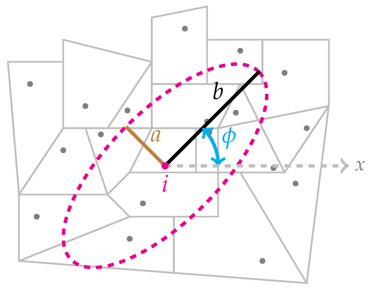
In the elliptic scan method, the set ${\mathcal{Z}}_e$ consists of many overlapping ellipses; each ellipse is characterized by (i) the x-coordinate and y-coordinate of its origin i, (ii) its shape s, (iii) its angle $\varphi$, and (iv) its population size. The shape $s\ge 1$ of an ellipse is defined as the ratio of the major axis and minor axis. A window with $s=1$ is a special case of an ellipse that represents a circle, and as s gets larger, the ellipse becomes narrower and longer. The collection of ellipse shapes recommended by Kulldorff et al. [12] is $s=$ 1, 1.5, 2, 3, 4, 5, 6, 8, 10, 15, 20, 30, 60, 120. The parameter $\varphi$ is the angle between the major axis and the x axis. Figure 1 displays an ellipse and its associated parameters.

For a fixed center, shape s, and population size, we can define the set of angles $\varphi$ such that a new ellipse overlaps at least 70% of the previous ellipse. To construct a set of candidate zones, ${\mathcal{Z}}_e$, for a region with a fixed center located at $(x,y)$, shape s, and angle $\varphi$, we successively enlarge the size of the ellipse (though shape s is fixed) until the stopping criterion is met, which is typically including no more than 50% of the total population in the ellipse. Each time a new centroid falls inside the ellipse, a new candidate zone is created by taking the union of all regions with a centroid inside the ellipse. We repeat this process for all different user-specified combinations of centers, shapes, and angles.

To conduct hypothesis testing, both ${\lambda }_{\mathbf{Z}}^c$ and ${\lambda }_{\mathbf{Z}}^{{}^{\prime }c}$ in Equations (4) and (6) can be used as LRT statistics. However, using these unpenalized statistics may cause the detection of impractically long and narrow ellipses. Thus, Kulldorff et al. [12] suggested an eccentricity penalty function that penalizes very thin clusters. The eccentricity penalty is ${\left(4s{(s+1)}^{-2}\right)}^{\gamma }$, where s is the shape of the cluster and $\gamma \ge 0$ is a tuning parameter. Therefore, the likelihood ratio test statistic for Poisson case counts in the elliptic scan method is given by

$${\lambda }^e=\underset{\mathbf{Z}\in {\mathcal{Z}}_e}{sup}{\left({\displaystyle \frac{y_{in}}{E_{in}}}\right)}^{y_{in}}{\left({\displaystyle \frac{y_{out}}{E_{out}}}\right)}^{y_{out}}I\left({\displaystyle \frac{y_{in}}{E_{in}}}>{\displaystyle \frac{y_{out}}{E_{out}}}\right){\left({\displaystyle \frac{4s}{{(s+1)}^2}}\right)}^{\gamma }.$$

(8)

when $s=1$ or $\gamma =0$, there is no penalty. For a fixed $s>1$, as $\gamma$ gets larger, a larger penalty is imposed on the model. Similarly, for a fixed $\gamma >0$, as s gets larger, a larger penalty is imposed on the model, so long and narrow clusters are less likely to be detected. When $\gamma \to \infty$, penalties for non-circular clusters are very large and only circular clusters can be detected. The same penalty function can be used for the Binomial case counts LRT given in Equation (6). In the following sections, we focus only on the Poisson case counts. However, any LRT statistic modification can be applied to the binomial case counts as well.

The elliptic scan method is relatively fast, powerful, and suited for moderately irregular clusters. However, the elliptic scan method also has many unknown parameters such as shape s, angle $\varphi$, population size, and tuning parameter $\gamma$ that should be specified by users. For real data sets in which the true clusters are unknown, picking the right parameters is not simple, and using different parameters has a significant impact on the final results and decisions. Furthermore, because the set ${\mathcal{Z}}_e$ includes only ellipses, the elliptic method is unable to detect highly irregular cluster shapes, e.g., star-like shape clusters.

2.3. The Flexible Scan Method

The flexible spatial scan method proposed by Tango and Takahashi  [7] is able to detect non-circular clusters by exhaustively searching all of the connected candidate zones within neighborhoods that include up to K regions. Given K, for every region $i\in \{1,\dots ,N\}$ the set of the candidate zones ${\mathcal{Z}}_f$ is the union of all connected subsets among the K nearest neighbors of i that include region i. The algorithm that Tango and Takahashi [7] proposed for constructing the connected regions within a circle with radius K is as follows:

• For each region $i\in \{1,\dots ,N\}$, define the set $W_i=\{i,i_1,\dots ,i_k\}$ such that $i_k$ is the kth nearest region to the region i.
• Let $\mathbf{Z}$ be a set in the power set of $W_i$ (i.e., $\mathbf{Z}\in \mathcal{P}\left(W_i\right)$) which includes region i. Therefore, $\mathbf{Z}$ is a set that has at most $k+1$ regions including centroid i. For example, $\mathbf{Z}=\{i,i_2,i_8,i_5,\dots ,i_{k^{\prime }}\}$, where $k^{\prime }\le k$.
• Split the set $\mathbf{Z}$ into two subsets ${\mathbf{Z}}_1^{\ast }=\left\{i\right\}$ and ${\mathbf{Z}}_1=\mathbf{Z}\setminus {\mathbf{Z}}_1^{\ast }$.
• Split set ${\mathbf{Z}}_1$ to two subsets ${\mathbf{Z}}_2$ and ${\mathbf{Z}}_2^{\ast }$ such that ${\mathbf{Z}}_2^{\ast }$ contains all the regions of ${\mathbf{Z}}_1$ that are connected to set ${\mathbf{Z}}_1^{\ast }$, and ${\mathbf{Z}}_2$ contains all the regions that are not connected to ${\mathbf{Z}}_1^{\ast }$. The process continues until either ${\mathbf{Z}}_j^{\ast }$ or ${\mathbf{Z}}_j$ becomes a null set for a $j\in \mathbb{N}$.
• $\mathbf{Z}$ in Step 2 is a connected set of regions if ${\mathbf{Z}}_j$ in Step 4 becomes a null set first, otherwise $\mathbf{Z}$ is disconnected.
• If $\mathbf{Z}$ in Step 5 is a connected set, it will be added to ${\mathcal{Z}}_f$.
• Repeat Steps 1 through 6 for all regions i and all sets $\mathbf{Z}\in \mathcal{P}\left(W_i\right)$.

Once the set of candidate zones ${\mathcal{Z}}_f$ is formed, the LRT statistic ${\lambda }_{\mathbf{Z}}^c$ Equation (4) (for the Poisson case counts) is calculated for each $\mathbf{Z}\in {\mathcal{Z}}_f$, and the one that attains the maximum is the MLC. Compared to the circular and elliptic scan method, this method can detect highly irregular clusters within small neighborhood sizes. Since the number of candidate zones increases exponentially as a function of K, this method is not computationally feasible for large K like $K\ge 30$ [7]. Additionally, in those situations where the true cluster is circular, the flexible method tends to detect clusters larger than the true cluster. In the next section, we describe the restricted flexible scan method, which attempts to address these limitations.

2.4. The Restricted Flexible Scan Method

Due to the computational inefficiency of the flexible scan method, Tango and Takahashi [8] proposed the restricted flexible (rflex) scan method to decrease the computation time needed for detecting larger clusters. In order to avoid adding low-risk regions to the set of candidate zones, for each region $\mathbf{Z}\in {\mathcal{Z}}_f$, Tango and Takahashi proposed the following restricted likelihood ratio by taking the risk of each individual region into account:

$${\lambda }_{\mathbf{Z}}^r={\left(\frac{y_{in}}{E_{in}}\right)}^{y_{in}}{\left(\frac{y_{out}}{E_{out}}\right)}^{y_{out}}I\left(\frac{y_{in}}{E_{in}}>\frac{y_{out}}{E_{out}}\right)\prod _{i\in \mathbf{Z}}I(p_i<{\alpha }_1),$$

(9)

where ${\alpha }_1$ is a pre-specified significance level and $p_i$ is the middle p-value given by

$$p_i=P\left(Y_i\ge y_i+1\right)+\frac{1}{2}P\left(Y_i=y_i\right),$$

(10)

where $y_i$ is the observed case count for region i, $Y_i\sim \mathrm{Poisson}\left(n_{i}r\right)$, and $r=y_{+}/n_{+}$ is an estimate of constant risk. For a low-risk region $i\in \mathbf{Z}$, the indicator function $I(p_i<{\alpha }_1)$ is zero and then the entire candidate zone $\mathbf{Z}$ is considered insignificant, meaning that it will be removed from the set of candidate zones ${\mathcal{Z}}_f$. Removing low-risk zones from the set of candidate zones ${\mathcal{Z}}_f$ makes the computational load lighter than the original method. Tango and Takahashi [8] provided the following guidance regarding the choice of ${\alpha }_1$ as follows:

• $0.10\le {\alpha }_1<0.20$ for detecting small clusters,
• $0.20\le {\alpha }_1<0.30$ for detecting small to medium clusters,
• $0.30\le {\alpha }_1<0.40$ for detecting large clusters.

The tuning parameter ${\alpha }_1$ is an unknown parameter that must be specified by users that will directly impact the results and performance of the restricted method. Moreover, even though the restricted flexible method has a lighter computational load than the original flexible method, it may still be computationally demanding for large ${\alpha }_1$.

2.5. The Flexible-Elliptical Scan Method

We now describe the flexible–elliptical scan method. The flexible–elliptical method is characterized by (i) the set of candidate zones ${\mathcal{Z}}_{fe}$ (the subscript “fe” stands for flexible–elliptical) and (ii) the LRT statistic ${\lambda }^{fe}$. Since Tango and Takahashi [7,8] create candidate zones from subsets of connected regions in concentric circles having K regions, highly irregular and long clusters may be difficult to detect unless K becomes large. More specifically, K might need to be very large before the irregular cluster contained in a concentric circle of K nearest neighbors. Furthermore, the set of elliptic candidate zones ${\mathcal{Z}}_e$ is not versatile enough to cover non-elliptical clusters. To form a larger and more flexible set of candidate zones, we construct the set of candidate zones based on the set of all connected subsets within the elliptical windows. In other words, for a fixed region i, fixed shape s, and fixed angle $\varphi$, first we sequentially enlarge the ellipsis until a stopping criterion is met; inside the largest ellipse, we find all connected subsets that include region i.

The circular and elliptic scan methods tend to detect clusters larger than the true cluster because their candidate zones absorb low-risk regions as they become larger. In order to eliminate low-risk regions from ${\mathcal{Z}}_{fe}$, we adjust the LRT statistic in Equation (4) so that a region is only included in a candidate zone if its standardized mortality ratio (SMR) is at least 1. More formally, $\mathbf{Z}$ remains in ${\mathcal{Z}}_{fe}$ if $Y_i/E_i>1$ for all $i\in \mathbf{Z}$; however, $\mathbf{Z}$ is removed from ${\mathcal{Z}}_{fe}$ if $Y_i/E_i\le 1$ for some $i\in \mathbf{Z}$. Thus, we specify the LRT statistic for the flexible–elliptical method as

$${\lambda }_{\mathbf{Z}}^{fe}={\left(\frac{y_{in}}{E_{in}}\right)}^{y_{in}}{\left(\frac{y_{out}}{E_{out}}\right)}^{y_{out}}I\left(\frac{y_{in}}{E_{in}}>\frac{y_{out}}{E_{out}}\right)\prod _{i\in \mathbf{Z}}I\left(\frac{Y_i}{E_i}>1\right).$$

(11)

Considering Equation (11), if only one region i has fewer observed cases than what is expected, then the product ${\prod }_{i\in \mathbf{Z}}I(Y_i/E_i>1)$ becomes zero and the entire candidate zone $\mathbf{Z}$ is removed from ${\mathcal{Z}}_{fe}$. Removing low-risk candidate zones from the set ${\mathcal{Z}}_f$ will reduce the computation time compared to the unrestricted method. Additionally, the flexible–elliptical method may consider fewer candidate zones than the rflex method when ${\alpha }_1$ is relatively large (e.g., ${\alpha }_1\ge 0.40$), making it faster to apply. Unlike the restricted LRT statistic ${\lambda }^r$ in Equation (9), which requires an additional unknown parameter ${\alpha }_1$ in the model, the proposed LRT statistic in Equation (11) does not require any additional tuning parameter. This is helpful because the size of the true cluster is unknown, making it difficult to choose an appropriate ${\alpha }_1$.

We also can use a different adjustment to the LRT statistic ${\lambda }_{\mathbf{Z}}^{fe}$ in Equation (11) to eliminate low risk regions. To accomplish that, let $g_i=Y_i/E_i$, $i\in \{1,\dots ,N\}$ denote the empirical region rate and $\overline{g}=\frac{1}{N}{\sum }_{i=1}^N{g}_i$. Instead of using the multiplier ${\prod }_{i\in \mathbf{Z}}I\left(Y_i/E_i>1\right)$ in Equation (11), we can use ${\prod }_{i\in \mathbf{Z}}I\left(g_i>\overline{g}\right)$. For the data sets used in the simulation study section (Section 3), we get almost identical results. Due to this, in Section 3, we only provide the results of the flexible–elliptical method when using the LRT statistic in Equation (11).

3. Simulation Study

To assess the performance of the elliptic scan method, we compare its results to the elliptic and rflex scan method using non-circular benchmark data sets provided by Duczmal et al. [24]. The benchmark data sets are simulated based on the female breast cancer mortality in the $N=245$ counties (or county equivalent) in the northeastern United States during the years 1988–1992 [25]. Eleven clustering models “a” through “k” are generated such that the total number of cases across the study area is $y_{+}=600$ among $n_{+}=$29,535,210 people at risk. 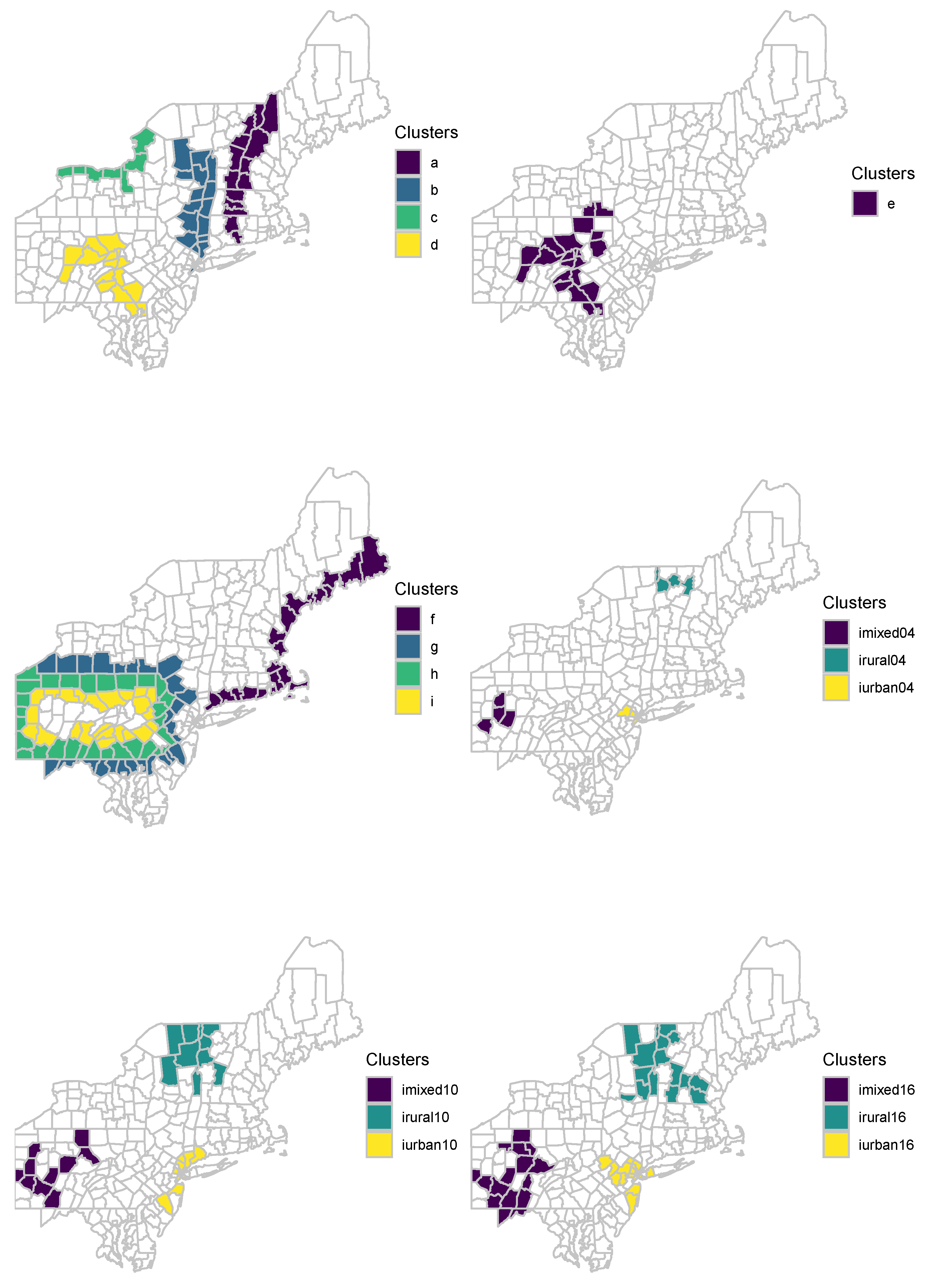Figure 2 illustrates clustering models “a”–“i”. Cluster “j” is the union of “g” and “h”. Cluster “k” is the union of “g”, “h”, and “i”. For each clustering model mentioned above, 10,000 different data set are generated. Additionally, 99,999 data sets are simulated under the null hypothesis of no clustering. These benchmark data sets are available in the neastbenchmark R package, which can be installed from https://github.com/jfrench/neastbenchmark (accessed on 7 July 2023).

To have a more extensive comparison, we generated 45 irregularly shaped clustering models based on circular benchmark data sets provided by Kulldorff et al. [25]. Three different sets of irregularly shaped clustering models, iurban (i.e., irregularly shaped urban clustering model), irural (i.e., irregularly shaped rural clustering model), and imixed (i.e., irregularly shaped mixed of urban and rural clustering models) are generated. Each clustering model contains 2–16 regions (counties). For each clustering model mentioned above, 10,000 different data set are generated. The last three plots of Figure 2 illustrate nine of these 45 clustering models.

To evaluate how well a cluster identified by each scan method matches the true cluster, different performance measures can be used [7,16]. We compare the methods in terms of their sensitivity, PPV, and misclassification as described below. Let z and $\widehat{z}$ denote the true cluster and the detected cluster, respectively. Let $n\left(X\right)$ be the population inside any zone X. Sensitivity is the proportion of the population of the true cluster that is covered by the detected cluster and is computed as

$$\mathrm{sensitivity}=\frac{n(z\cap \widehat{z})}{n\left(z\right)}.$$

(12)

PPV is the proportion of the population of the detected cluster that is covered by the true cluster and is computed as

$$\mathrm{PPV}=\frac{n(z\cap \widehat{z})}{n\left(\widehat{z}\right)}.$$

(13)

Misclassification is the proportion of the total population that is not correctly categorized and is computed as

$$\mathrm{misclassification}={\displaystyle \frac{n[(z\cup \widehat{z})\cap {(z\cap \widehat{z})}^c]}{n_{+}}}.$$

(14)

Ideally, we want to see sensitivity and PPV equal to 1 and misclassification equal to 0.

We compare the performance of the flexible–elliptical, rflex (for both tuning parameters ${\alpha }_1=0.2$ and ${\alpha }_1=0.3$), and elliptic scan method in terms of the average sensitivity, PPV, and misclassification. The smerc R package [26] was used to apply the elliptic and rflex methods to the benchmark data sets. Each scan method was applied to 1000 simulated data sets for each of the 56 clustering models. To keep the set of candidate zones more comparable for all three scan methods, the stopping criterion for the size of the scanning windows was set to K-nearest neighbors. That is, for each starting region, i, a maximum of $K-1$-nearest neighbors can be added. The rflex scan method used the middle p values, and the tuning parameters were set to ${\alpha }_1=0.2$ and ${\alpha }_1=0.3$. Both the elliptic and the flexible–elliptical methods used the default shape and angle values used in the SaTScan^TM software [27]. More specifically, the shapes are $s=1,1.5,2,3,4,5$, and the number of angles associated with each shape is $\varphi =1,4,6,9,12,15$. Therefore, for each region i, 47 different elliptical windows are considered; then, each of 47 elliptical shapes is enlarged until $K=20$ regions are included. All methods identified the clusters using the corresponding version of the LRT statistic in Equations (8), (9) and (11), respectively.

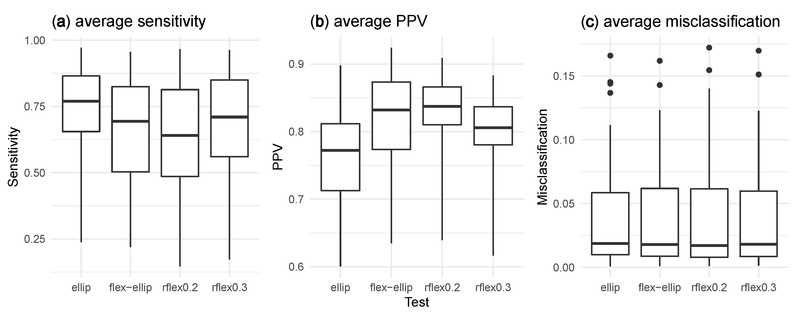
Figure 3 presents box plots of the average sensitivity, PPV, and misclassification for each method among all 56 clustering models. Table S1 in the Supplementary Materials provides complete results for the simulation study. Overall, the sensitivity of the elliptic method is higher than the other methods. This heightened sensitivity may be attributed to the fact that the elliptic method has a tendency to detect clusters that are larger than the true clusters. By detecting larger clusters, the elliptic method captures a greater number of true positives, resulting in a higher sensitivity value. However, it is important to note that this enhanced sensitivity comes at the cost of potentially including some false positives in the identified clusters. In contrast, the flexible–elliptical demonstrates a more consistent sensitivity and PPV across all different clustering models. Unlike the rflex method, which exhibits varying results based on the chosen value of ${\alpha }_1$, the flexible–elliptical method achieves a more constant sensitivity and PPV across different clustering models. Additionally, the flexible–elliptical method does not suffer from unnecessarily detecting larger clusters like the elliptic method. While the flexible–elliptical method may not always surpass the rflex and elliptic methods individually, it provides a robust and stable performance compared to the other two methods. The flexible–elliptical method exhibits similar sensitivities to the rflex method with ${\alpha }_1=0.3$, showcasing its overall robust performance. In terms of PPV, on average, the rflex method with ${\alpha }_1=0.2$, and the flexible–elliptical method demonstrate the highest average PPV values among the tested methods. This underscores the effectiveness of the flexible–elliptical method in identifying true clusters while minimizing false positives compared to the elliptic method. On the other hand, the elliptic method exhibits a relatively lower PPV, highlighting the advantages offered by the flexible–elliptical method in achieving precise and reliable cluster identification. Regarding misclassification, the results indicate similar average levels across all clustering models for each method.

4. Application to Northeastern United States Data

We now detect clusters of breast cancer mortality cases in the northeastern United States during the years 1988–1992. This data set is the inspiration for the simulated data examined in the previous section. We compare the clusters identified by the elliptic, rflex, and flexible–elliptical scan methods. The total number of observed breast cancer mortality cases is $y_{+}=$ 58,943, which was aggregated across the years 1988–1992. The population of each region used in this analysis is the 1990 U.S. census estimate, with the total number of persons at risk being $n_{+}=$ 29,535,210. More information related to the northeastern data set can be found in Kulldorff et al. [25].

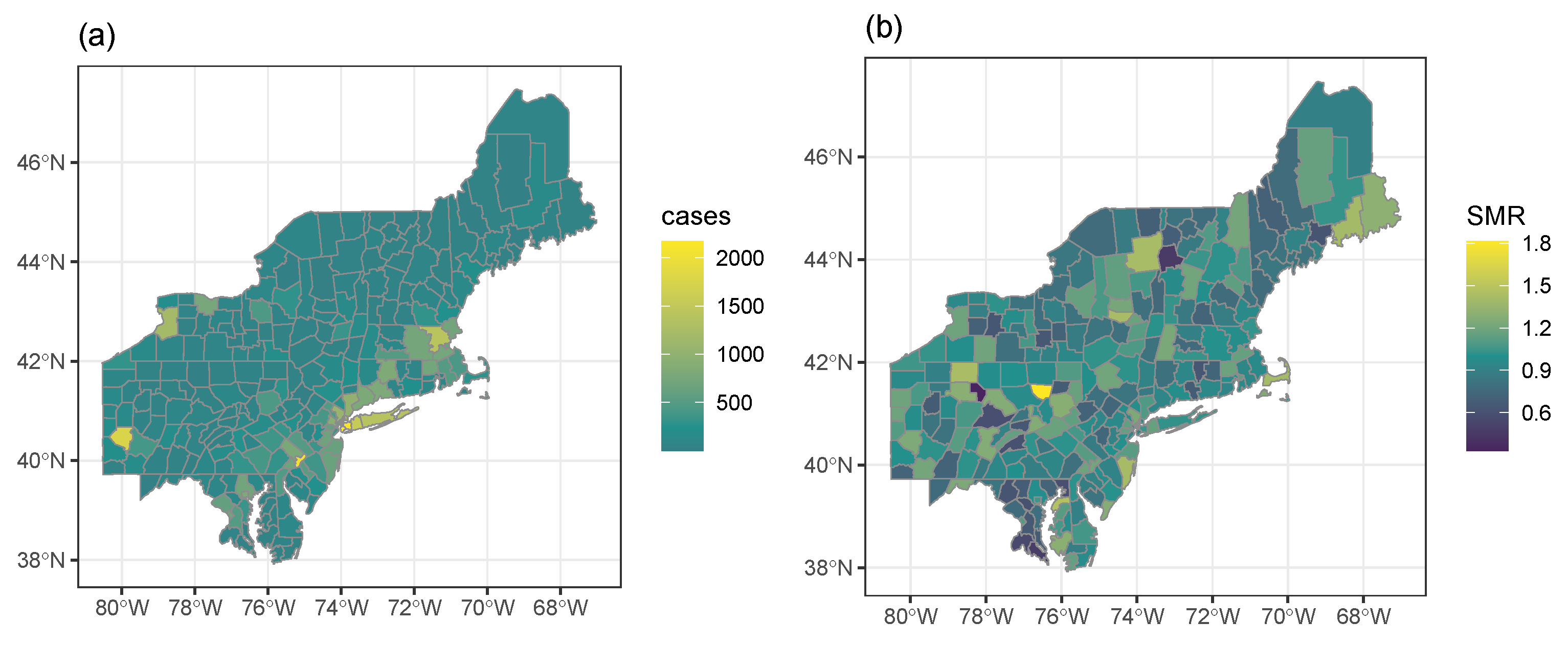
Figure 4 provides choropleth maps of the case count (left panel) and SMR (right panel) for each region in the northeastern data set. The number of cases per region ranged from 2 to 2169 with a median of 86 cases. The SMR of each region is computed as ${\mathrm{SMR}}_i=Y_i/E_i$, where $E_i$ is the population size of each region multiplied by the $\mathrm{constant}\mathrm{risk}=y_{+}/n_{+}$. The SMRs of the regions ranged from 0.33 to 1.81, while the case count plot in the left panel of Figure 4 does show patterns of large case counts, it is not clear whether this pattern is unusual because the plot does not account for the population size of each region. The SMR plot in the right panel of Figure 4 does not indicate any systematic patterns of high SMRs. Therefore, spatial scan methods must be applied to this data set to identify clusters.

The northeastern data were analyzed using the previously discussed scan methods, each of which identified different clusters. The maximum number of regions allowed in each candidate zone was set to $K=20$. The default values of s and $\varphi$ provided in Section 3 are used for the elliptic and flexible–elliptical method. For the middle p-value, two tuning parameters ${\alpha }_1=0.2$ and ${\alpha }_1=0.3$ were considered for the rflex method. For the elliptic method, $\gamma =0$ was used for the penalty function in Equation (8).

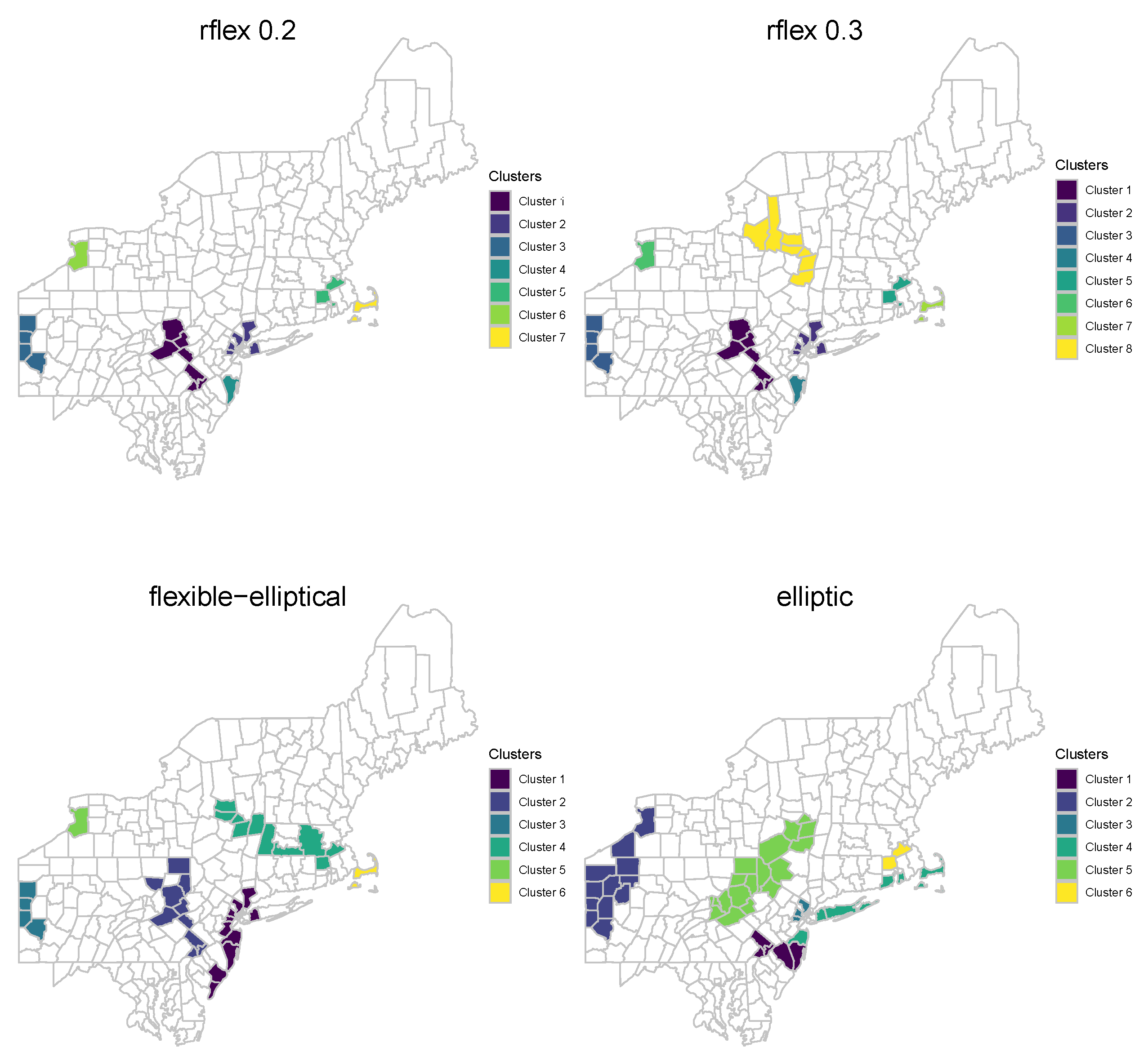
Figure 5 displays clusters detected by each scan method. There are seven clusters identified by the rflex method using ${\alpha }_1=0.2$. Eight clusters are detected by the rflex method using ${\alpha }_1=0.3$. Six clusters are detected by the elliptic and flexible–elliptical scan method. A summary of the significant clusters found at level $\alpha =0.05$ is given in

Table 1. Significant clusters detected by the rflex method (both ${\alpha }_1=0.2$ and ${\alpha }_1=0.3$), flexible–elliptical (flex-ellip) method, and elliptic method. The Monte Carlo p-value was computed using 999 null data sets under the constant risk hypothesis at the significance level of $\alpha =0.05$.

Method	Cluster	Population	Cases	Expected	SMR	p-Value
rflex (${\alpha }_1=0.2$)	Cluster 1	1,922,489	4525	3836	1.18	0.001
	Cluster 2	2,232,866	5150	4456	1.16	0.001
	Cluster 3	920,991	2248	1838	1.22	0.001
	Cluster 4	228,322	643	455	1.41	0.001
	Cluster 5	660,581	1537	1318	1.17	0.001
	Cluster 6	507,044	1201	1011	1.19	0.001
	Cluster 7	104,057	291	207	1.40	0.003
		mean = 939,478	mean = 2228		mean = 1.25
rflex (${\alpha }_1=0.3$)	Cluster 1	1,922,489	4525	3836	1.18	0.001
	Cluster 2	2,232,866	5150	4456	1.16	0.001
	Cluster 3	920,991	2248	1838	1.22	0.001
	Cluster 4	228,322	643	455	1.41	0.001
	Cluster 5	660,581	1537	1318	1.17	0.001
	Cluster 6	507,044	1201	1011	1.19	0.001
	Cluster 7	104,057	291	207	1.40	0.004
	Cluster 8	470,397	1084	938	1.15	0.041
		mean = 880,843	mean = 2085		mean = 1.23
flex-ellip	Cluster 1	3,256,369	7480	6498	1.15	0.001
	Cluster 2	2,062,671	4853	4116	1.18	0.001
	Cluster 3	920,991	2248	1838	1.22	0.001
	Cluster 4	1,673,793	3703	3340	1.11	0.001
	Cluster 5	507,044	1201	1011	1.19	0.004
	Cluster 6	104,057	291	207	1.40	0.009
		mean = 1,420,821	mean = 3296		mean = 1.21
elliptic	Cluster 1	1,917,315	4517	3826	1.18	0.001
	Cluster 2	1,701,906	3979	3396	1.17	0.001
	Cluster 3	1,102,261	2598	2199	1.18	0.001
	Cluster 4	1,841,814	4062	3675	1.11	0.001
	Cluster 5	889,355	2035	1774	1.15	0.002
	Cluster 6	635,396	1480	1268	1.17	0.002
		mean = 1,348,008	mean = 3112		mean = 1.16

.

The flexible–elliptical method exhibits several key properties that are worth focusing on. Notably, the clusters detected by this method encompass a larger number of cases, on average, compared to both the elliptic and rflex methods. Furthermore, the clusters identified by the flexible–elliptical method tend to have the largest population at risk, indicating their significance in terms of potential public health impact. While the rflex methods tend to yield clusters with higher SMR values, the flexible–elliptical method demonstrates slightly smaller SMR values, reflecting its ability to capture clusters with more precise risk estimates. In contrast, the elliptic method, which has a tendency to include low-risk regions, yields the lowest mean SMR values among the methods even though the population at rick is not as high as the flexible–elliptical method. This again shows a balancing of the advantages of both rflex and elliptic method. For example, consider Cluster 1 detected by the flexible–elliptical method. This cluster encompasses the largest population at risk compared to other clusters. Intriguingly, the rflex method detects two smaller clusters, namely Clusters 2 and 4, which, when combined, form a subset of Cluster 1. This example demonstrates that the flexible–elliptical method is capable of identifying more extensive and impactful clusters when compared to multiple smaller clusters detected by the rflex method.

Furthermore, Cluster 1 detected by the flexible–elliptical method was disconnected into two separate clusters, namely Cluster 1 and Cluster 4, by the elliptic method. This could be due to its ability to detect clusters of various shapes and sizes, making it more flexible and realistic in capturing different types of clusters. In contrast, the elliptic method tends to identify more compact and elliptical-shaped clusters. Almost all of the clusters detected by the elliptic method in Figure 5 have elliptical shapes, which might be unlikely in reality. It is important to note that, since the data set is real, definitive conclusions regarding the nature of the clusters cannot be made. However, the results from the proposed flexible–elliptical method demonstrate its ability to provide more diverse and versatile cluster configurations while maintaining a high number of cases, SMR values, and populations at risk. This method strikes a balance between the characteristics of the rflex and elliptic methods, offering a more comprehensive approach to cluster detection and potentially yielding more meaningful and interpretable results.

5. Application to NTM Data

In order to provide a more extensive comparison, we also analyze nontuberculous mycobacterial (NTM) patient data and identify disease clusters by comparing the discussed three spatial scan approaches. NTM data were obtained from the National Jewish Health (NJH) Hospital electronic medical record database in Denver, Colorado. All patients (those with cystic fibrosis and those without) who had sought treatment at NJH, had a diagnosis of NTM infection (i.e., at least one positive culture) and were resident in Colorado during February 2008 through January 2018 were included in this dataset, totaling $y_{+}=822$ patients. Since NTM is considered a rare disease, we aggregated patient data over a 10-year period and tabulated patient data for each zip code tabulation area (ZCTA). We used the total population of Colorado as determined by the 2010 US Census, fixed at $n_{+}=$ 5,029,374 people. Given that the incubation period of NTM is not currently understood, we did not have a reliable time of disease onset variable, and therefore, we could not consider a temporal analysis to identify disease clusters. The use of this dataset was approved by the NJH Institutional Review Board (HS-3148).

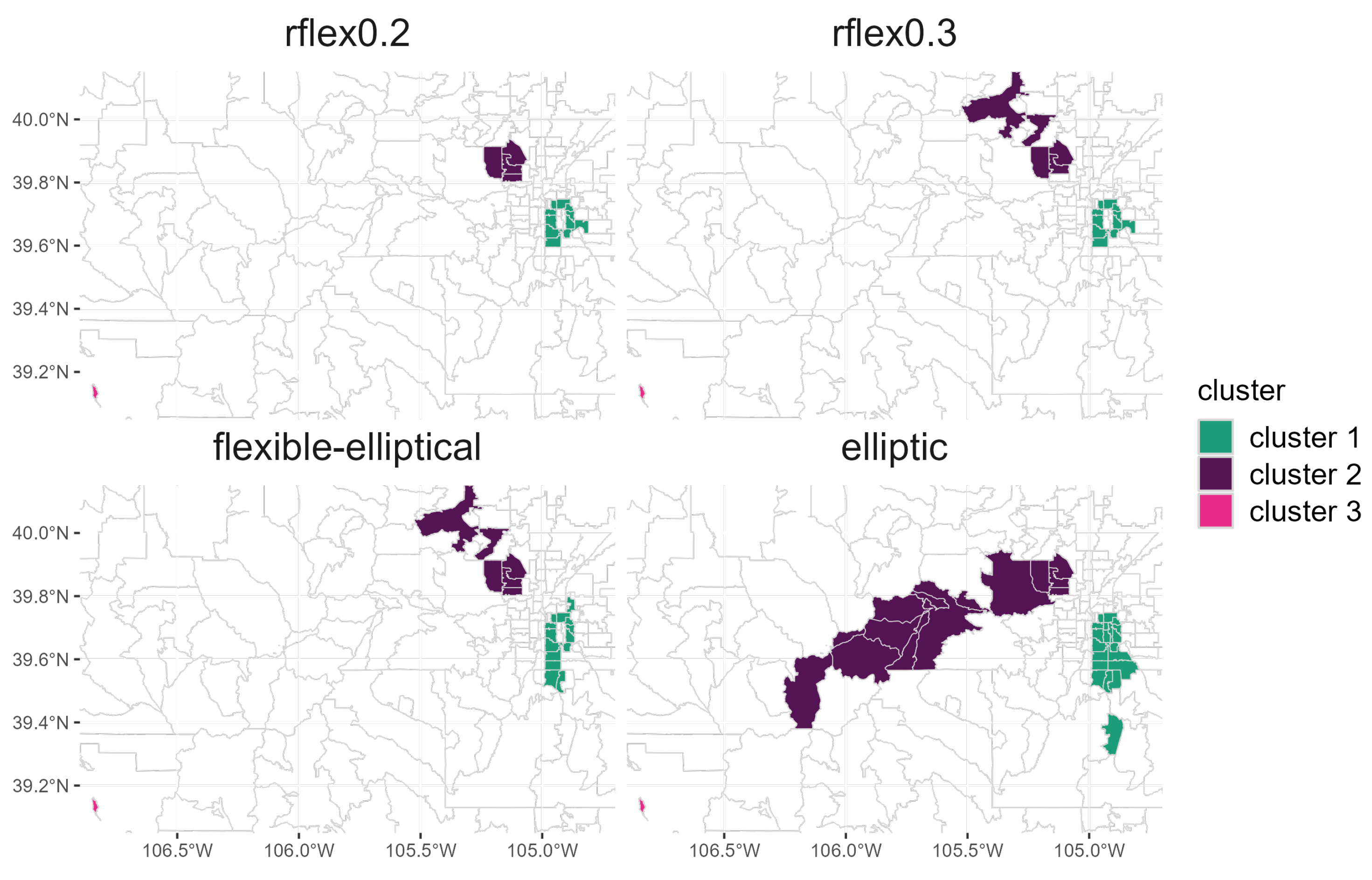
Figure 6 displays the significant NTM clusters detected by each scan method at significance level $\alpha =0.05$. To compute the p-value, 999 null data sets were simulated under constant risk hypothesis. The rflex method with ${\alpha }_1=0.2$ and ${\alpha }_1=0.3$ identified the same Cluster 1 but the rflex method with ${\alpha }_1=0.3$ includes additional regions for Cluster 2 compared to the rflex method with ${\alpha }_1=0.2$. For Cluster 1, the flexible–elliptical method included a longer, narrower set of zip codes compared to those identified by the rflex methods. For Cluster 2, the rflex methods differed from the flexible–elliptical method by only one zip code. The elliptic method detected the largest clusters among all of the methods tested. The elliptic method detected Cluster 1 zip codes within the same location as the previous methods but covered a larger area of zip codes. For Cluster 1, all methods identified some variation of zip codes within the center to the eastern end of the city of Denver and in suburban regions south of Denver. For Cluster 2, the elliptic method identified a much larger Cluster compared to those identified by the other methods. In Cluster 2, all methods included zip codes located in the city of Arvada. The rflex methods and the flexible–elliptical method also included zip codes located in Boulder County. The elliptic method did not include the Boulder zip codes but included the Arvada zip codes. Cluster 2, identified by the elliptic method, extended farther west into the Rocky Mountains. All methods detected Cluster 3, as this included one zip code in Pitkin County with only 20 residents.

NTM are commonly found in water, and the hypotheses surrounding NTM exposure and acquisition focus on municipal water supplies. The water supply for zip codes located in Cluster 1 comes from different regions along the Western Slope than for zip codes located in Cluster 2 (for clusters identified by the rflex and flexible–elliptical methods). Recent studies have demonstrated an association between a trace metal, molybdenum, in the raw water supply and NTM infection risk in Colorado [28,29]. Regions that supply water to zip codes in Clusters 1 and 2 have naturally occurring molybdenum in high abundance, as evidenced by the fact that large molybdenum mines are located in these regions. These regions with high molybdenum concentrations are located within Cluster 2 identified by the elliptic method.

The rflex method and the flexible–elliptical method present zip codes in Boulder County and the city of Arvada as part of Cluster 2. The Boulder zip codes receive their water supply from sources that are different from the Arvada zip codes. Since the Boulder zip codes were not identified in the elliptic method cluster, this identification may lead us to further examine those regions.

The elliptic method, because it typically exhibits greater sensitivity, tends to generate clusters including more zip codes and that have larger geographic area. However, its detected clusters tend to have lower PPV as not all zip codes within the detected clusters are likely to be high risk. The rflex and flexible–elliptical methods typically have greater PPV, so they are likely more useful for identifying the highest risk regions within the true cluster. Given that its detected clusters tend to be larger, the elliptic method may provide more opportunities for hypothesis generation in the initial stages of data exploration, while the elliptic–flexible method possibly focuses in on the most high-risk regions of each cluster.

6. Conclusions

In our simulation study, it was revealed that the elliptic method generally displayed higher sensitivity compared to the other scan methods. This heightened sensitivity is attributed to the elliptic method’s tendency to detect larger clusters, increasing the chances of capturing the true cluster. In contrast, the rflex method with ${\alpha }_1=0.2$ exhibited the lowest sensitivity, likely due to the elimination of moderate-rate regions by the middle p-value. However, the sensitivity of the flexible–elliptical method closely aligned with that of the rflex method with ${\alpha }_1=0.3$, indicating its comparable performance in identifying irregularly shaped clusters. Importantly, the proposed flexible–elliptical method moderates the trade-off between cluster size and accuracy without relying on any specific tuning parameter, providing a more flexible and versatile approach to capturing the true cluster.

The simulation study also revealed that, on average, the flexible–elliptical method demonstrated a better performance based on PPV. The PPV of the rflex method with ${\alpha }_1=0.2$ was comparable to the flexible–elliptical method, but the rflex method with ${\alpha }_1=0.3$ resulted in lower PPV. The elliptic method had the lowest PPV values, which again could be attributed to its tendency to detect clusters larger than the true clusters. PPV ensures more accurate and reliable cluster identification, holding significant implications for the precision and validity of cluster detection studies. By effectively detecting and capturing clusters, the proportion of the detected clusters accurately aligning with the true clusters in the population increased, which is an important measure. This further highlights the flexible–elliptical method as a versatile approach to maintain high accuracy and impact in cluster detection while avoiding dependence on a tuning parameter and detecting excessively larger clusters.

Notably, the performance of the rflex method exhibits some inconsistency between the two ${\alpha }_1$ levels, 0.2 and 0.3. This observation practically implies that the effectiveness of the rflex method relies on the chosen value of ${\alpha }_1$ and the specific characteristics of the clustering model. For instance, when examining the clustering model “irural05”, the sensitivity ranges from 0.61 for ${\alpha }_1=0.20$ to 0.70 for ${\alpha }_1=0.30$, while the PPV ranges from 0.79 to 0.74, or the clustering model “iurban08”, the sensitivity ranges from 0.59 for ${\alpha }_1=0.20$ to 0.71 for ${\alpha }_1=0.30$, while the PPV ranges from 0.81 to 0.78.

The performance in terms of misclassification was generally comparable across all methods. This similarity arose from the definition of misclassification in Equation (14), where the denominator represented the total population at risk. The breast cancer data set in Section 3 had a large total population size of $n_{+}=$ 29,535,210, contributing to the similarity in misclassification rates. However, it is worth noting that the proposed flexible–elliptical method demonstrated improved performance in certain clustering models, such as models “j”, “k”, and “iurban13”.

7. Discussion

In this study, we proposed the flexible–elliptical scan method, which combined the flexible and elliptic scan methods to address their respective limitations and leverage their advantages. Our approach involved modifying the set of candidate zones and the likelihood ratio test statistics. We thoroughly compared the performance of the proposed flexible–elliptical method with the elliptic and rflex methods for identifying irregularly shaped disease clusters. This evaluation included benchmark data sets comprising 56 diverse irregularly shaped cluster models as well as real-world data sets related to breast cancer mortality and NTM cases. Our findings demonstrated a balanced performance between the flexible and elliptic scan methods in accurately detecting irregularly shaped clusters in disease surveillance.

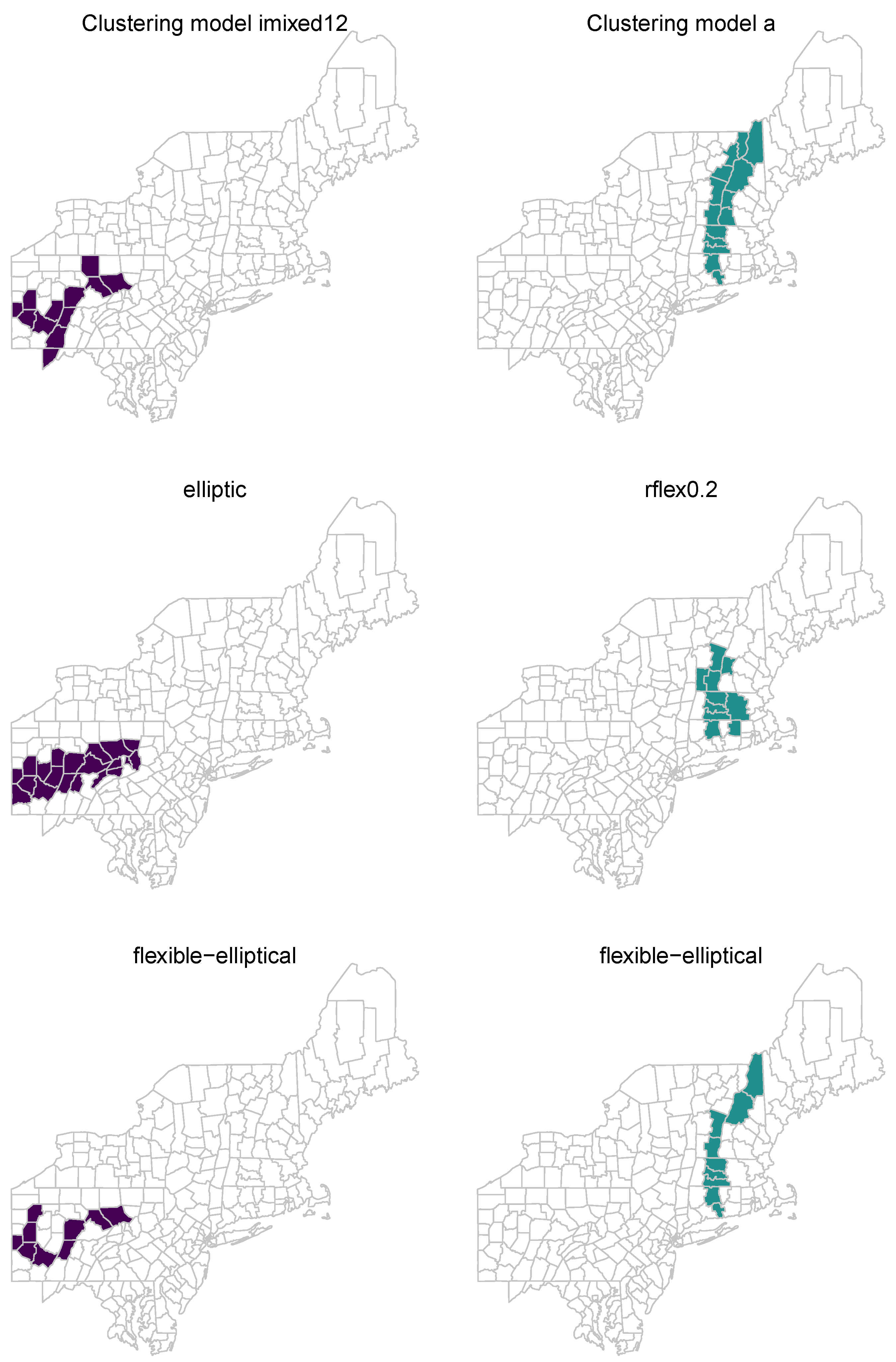
The flexible–elliptical method exhibited flexibility, inheriting the capabilities of the rflex and elliptic methods, particularly in constructing the set of candidate zones. The elliptic method often struggled to identify clusters with highly irregular shapes, limiting its effectiveness in capturing complex disease patterns. Similarly, the rflex method faced challenges in detecting very long and narrow clusters due to its reliance on circular-shaped windows and the user-defined ${\alpha }_1$ tuning parameter. By incorporating the strengths of these two methods, the flexible–elliptical method demonstrated a more adaptable approach to candidate zone construction, enabling it to capture highly non-circular shaped clusters as shown in Figure 7. This heightened flexibility allowed for the detection of a broader range of cluster shapes, rendering the flexible–elliptical method a valuable tool in identifying irregular disease clusters and leveraging the advantages of both elliptic and reflex methods.

While the rflex method’s performance can vary depending on the chosen tuning parameter values, the proposed flexible–elliptical method eliminates the need for such parameter adjustments. The flexible–elliptical method demonstrates independence from tuning parameters, ensuring consistent and reliable cluster detection outcomes. While the rflex method with tuning parameters ${\alpha }_1=0.2$ and ${\alpha }_1=0.3$ exhibited relatively good sensitivity and PPV, a closer examination reveals that ${\alpha }_1=0.2$ yielded a superior PPV, whereas ${\alpha }_1=0.3$ achieved better sensitivity (Figure 3). Moreover, the number of significant clusters can be influenced by the choice of tuning parameter (e.g., Figure 5). On the other hand, the elliptic method imposed an eccentricity penalty on the likelihood ratio test statistic which required another tuning parameter. By adjusting the tuning parameter, the elliptic method avoided detecting very narrow and long clusters. In the proposed flexible–elliptical method, no eccentricity penalties have been used. First, we considered not only elliptical windows but also connected regions inside them. Second, we filtered out windows having low-risk regions. Therefore, even if a very narrow and thin cluster is obtained, an additional penalty is not required due to the fact that we include only high-risk regions in each cluster. An example of such a cluster can be found in the bottom-right plane of Figure 7, which is a very long cluster, as it should be.

The flexible–elliptical method avoids including low-risk regions, which could potentially be an advantage, but it does allow for disconnecting a large cluster. For example, consider two large significant clusters that are connected with a single region, and that region is a low-risk region. In this situation, the flexible–elliptical method presumably detects one of them. It is possible that the other cluster is detected as a secondary cluster, but it is not guaranteed. It is important to note that there were some situations where the elliptic method detects clusters containing disconnected regions. For example, in the clustering models such as Cluster “c” in Figure 2, the nearest neighbors are not necessarily connected, and elliptical windows may include disconnected regions. Another example is shown in Cluster 1 detected by the elliptic method in Figure 6. Unlike the elliptic method, the flexible–elliptical method disconnects regions systematically. This can be a limitation of the proposed flexible–elliptical method, and it could be extended when taking other criteria into account before removing a region only based on whether it is a low-risk region. Similar to algorithms proposed by Costa et al. [16], we may avoid eliminating those low-risk regions by having specific geographic proximity criteria. For example, consider a current window that involves only high-risk regions. We can let a low-risk region be added to this current window if the region has two connections (borders) and increases the current likelihood test statistic value. Furthermore, although the proposed method is relatively simple, it is possible to impose additional restrictions on the regions to further enhance speed and accuracy in Cluster detection.

In summary, the proposed method combines two well-known methods for detecting irregularly shaped clusters, taking advantage of their individual strengths and achieving a balanced approach. The flexible–elliptical method inherits the favorable features of both the elliptic and rflex methods. It demonstrates a better positive predictive value (PPV) compared to the elliptic method and comparable PPV to the rflex method with ${\alpha }_1=0.2$. Notably, the flexible–elliptical method does not rely on the tuning parameter ${\alpha }_1$, offering a more streamlined and straightforward approach. The construction of the set of candidate zones in the proposed method provides greater flexibility compared to the rflex method, allowing for improved adaptability to irregular cluster shapes.