Families of Extended Exponentiated Generalized Distributions and Applications of Medical Data Using Burr III Extended Exponentiated Weibull Distribution

Abstract

In this article, four new families named as Weibull extended exponentiated-X (WEE-X), Lomax extended exponentiated-X (LEE-X), Logistic extended exponentiated-X (LGCEE-X), and Burr III extended exponentiated-X (BIIIEE-X) with their quantile functions are proposed. The expressions for distribution function and density function of BIIIEE-X family are written in terms of linear combinations of the exponentiated densities based to parent model. New models, i.e., Weibul extended exponentiated Weibull (WEEW), Lomax extended exponentiated Weibull (LEEW), Logistic extended exponentiated Weibull (LGCEEW), and Burr III extended exponentiated-Weibull (BIIIEEW) distributions are derived, were plotted for functions of probability density and hazard rate at different levels of parameters. Some mathematical properties of the BIIIEEW model are disclosed. The maximum likelihood method for the BIIIEEW model are described. Numerical applications of the BIIIEEW model to disease of cancer datasets are provided.

1. Introduction

Statistical modeling of lifetime data plays an important role in medical science. To determine reliable results in estimating medical data, it is often required to choose the appropriate statistical distribution of the data. Continuous probability distributions, such as the Weibull, exponential, Rayleigh, lognormal, gamma, logistic, and log-logistic, can be used to model biomedical data (BoMD). However, it is clear that the BoMD deviate from these classical distributions because of the skewness and heavy tails that are present in the data. Due to this, the aforementioned traditional skewed distributions become less suitable for modeling BoMD. Weibull distribution (WD) is not flexible enough to handle data types with a lot of complexity. Practically all clinical issues, including breast, bladder, neck, and other cancers, have unimodel or modified unimodel failure rates. After surgery, risk of bladder, breast, and neck cancer are unimodel. The regular two-parameter WD can simply model monotonically increasing and decreasing failure rate functions (FRFs), making it less relevant for fitting when data show non-monotonic FRFs. These disadvantages have motivated researchers to develop several generalizations of it to obtain more flexible distributions for modeling. Therefore, there is a need to emphasize the importance of enhancing the classical distributions for modeling BoMD. Numerous studies have been conducted to create statistical models that are superior to conventional models in their ability to describe health data.

Based on extended versions of WDs, numerous studies have examined the characteristics of various cancer datasets (CDSs). When data on cancer remission times were applied, the q-Weibull distribution by Jose and Naik (2009) [1] performed better than the regular WD. When it came to modeling colorectal cancer, the generalized WD that was developed by Baghestani et al. (2017) [2] performed well. The performance of the beta- weighted WD described by Idowu and Ikegwu (2013) [3] was validated using bladder cancer datasets (BCDSs). Modeling BCDSs was used to evaluate the empirical proofs of the transmuted exponentiated generalized WD by Yousof et al. (2017) [4], the Marshall- Olkin generalized WD by Elgohari and Yousof (2020) [5], the Marshall–Olkin power generalized WD by Afify et al. (2020) [6], and the Gull alpha power WD by Ijaz et al. (2020) [7]. With these new families, statistical modeling can be more adaptable, especially in practical fields, such as finance, engineering, the environment, and health care. In the statistical literature, one can add one or more parameters to a known distribution to create a family of distributions. The generalized distribution emerges when the parameters are added to the baseline distribution. The generalized distribution can be used effectively in fitting lifetime datasets because it can accommodate monotonic and non-monotonic data characteristics.

The transformed-transformer (T-X) technique was proposed by Alzaatreh et al. (2013) [8] to develop new G-families. Let $T\in [t_1,t_2]$ for $-\infty \le t_1, t_2\le \infty$ be a random variable (rv) having probability density function (PDF) $\pi \left(t\right)$ and cumulative distribution function (CDF) $\mathsf{\Pi }\left(t\right)$ and let $\mathsf{\Phi }\left[G\right(x\left)\right]$ be a function of CDF $G\left(x\right)$ of any parent rv X so that $\mathsf{\Phi }\left[G\right(x\left)\right]$ satisfies the conditions below:

$$\left.\begin{array}{c}\hfill \mathsf{\Phi }\left[G\left(x\right)\right]\in [t_1,t_2],\\ \hfill \underset{x\to -\infty }{lim}\mathsf{\Phi }\left[G\left(x\right)\right]=t_1\mathrm{and}\underset{x\to +\infty }{lim}\mathsf{\Phi }\left[G\left(x\right)\right]=t_2,\\ \hfill \mathsf{\Phi }\left[G\right(x\left)\right]\mathrm{is}\mathrm{non}-\mathrm{decreases}\mathrm{monotone}\mathrm{and}\mathrm{differentiable}.\end{array}\right\}$$

(1)

The CDF of T-X family of distributions (FoDs) is:

$$\begin{array}{cc}{F}^{TX}\left(x\right)& ={\int }_{t_1}^{\mathsf{\Phi }\left[G\right(x\left)\right]}\pi \left(t\right)\mathrm{d}t,\hfill \\ & =\mathsf{\Pi }\left(\mathsf{\Phi }\left[G\right(x\left)\right]\right).\hfill \end{array}$$

(2)

The PDF associated with Equation (2) is:

$$f^{TX}\left(x\right)=\pi \left(\mathsf{\Phi }\left[G\right(x\left)\right]\right)\frac{\mathrm{d}}{\mathrm{d}x}\mathsf{\Phi }\left[G\left(x\right)\right].$$

(3)

In Equation (2), the PDF $\pi \left(t\right)$ is transformed into CDF $F^{TX}\left(x\right)$ by function $\mathsf{\Phi }\left[G\right(x\left)\right]$, which behaves similar to a transformer, and in Equation (3), the distribution $f^{TX}\left(x\right)$ is transformed from rv T through transformer rv X.

The function $\mathsf{\Phi }\left[G\right(x\left)\right]$ will give a new FODs based on the support of the rv T. By using the following equation:

$$\mathsf{\Phi }\left[G\left(x\right)\right]=-log\left\{\frac{1-G^{\theta }\left(x\right)}{1-log[1-G^{\theta }\left(x\right)]}\right\},$$

(4)

the $F^{TX}\left(x\right)$ in Equation (2) is a CDF of new FoDs, which is defined as:

$$F^{TX}\left(x\right)={\int }_0^{-log\left\{\frac{1-G^{\theta }\left(x\right)}{1-log[1-G^{\theta }\left(x\right)]}\right\}}\pi \left(t\right)\mathrm{d}t=\mathsf{\Pi }\left(-log\left\{\frac{1-G^{\theta }\left(x\right)}{1-log[1-G^{\theta }\left(x\right)]}\right\}\right),$$

(5)

where $\mathsf{\Pi }\left(t\right)$ is the CDF of rv T. The corresponding PDF related to Equation (5) is:

$$f^{TX}\left(x\right)=\frac{\theta g\left(x\right)G^{\theta -1}\left(x\right)}{1-G^{\theta }\left(x\right)}\left[1+\frac{1}{1-log[1-G^{\theta }\left(x\right)]}\right]\pi \left(-log\left\{\frac{1-G^{\theta }\left(x\right)}{1-log[1-G^{\theta }\left(x\right)]}\right\}\right).$$

(6)

The main objectives for proposing new X-families are:

i.

Developing new X-families related to the function of CDF, i.e., $\mathsf{\Phi }\left[G\right(x\left)\right]$.

ii.

The developed families based on a generator, i.e., $-log\left\{\frac{1-G^{\theta }\left(x\right)}{1-log[1-G^{\theta }\left(x\right)]}\right\}$ instead of $G\left(x\right)$.

iii.

The generator discussed in step ii has the ability to generate better goodness of fit results and parameters estimates that can make it distinguishable and attractive for the researcher.

The article is arranged as follows. Section 2 presents four new proposed T-X distribution families, such as the WEE-X family, LEE-X family, LGCEE-X family, and BIIIEE-X family with their quantile functions. In Section 2.1.1, Section 2.2.1, Section 2.3.1 and Section 2.4.1, submodels WEEW of the WEE-X family, LEEW of the LEE-X family, LGCEE of the LGCEE-X family, and BIIIEEW of the BIIIEE-X family are characterized by PDF and FRF plots. The useful expressions for BIIIEE-X family are derived in Section 3. For the BIIIEEW model, we derive few mathematical properties in Section 4. The estimation of BIIEEWD by the maximum likelihood method is explained analytically in Section 5. Section 6 describes the applications of the proposed model to different datasets of cancer disease. Lastly, the conclusion is drawn in Section 7.

2. Some New T-X Distributions Families with Different T Distributions

Based on the classification of the T-X family, two subfamilies can be identified: the first subfamily has different T distributions, but the same X distribution, while the second subfamily has different X distributions but the same T distribution. This section considers the subfamily of different T distributions with their submodels. Here, we considered Weibull, Lomax, Logistic, and Burr III as T distributions and Weibull as an X distribution.

2.1. Weibull Extended Exponentiated-X (WEE-X) Family

If an rv $T\sim$ Weibull distribution (WD) with $\gamma$ and $\alpha$ parameters, then $\mathsf{\Pi }\left(t\right)=1-e^{-\gamma t^{\alpha }}$, $t\ge 0$. From Equation (5), the CDF of the WEE-X family is:

$$F^{WEE-X}\left(x\right)=1-exp\left(-\gamma {\left[-log\left\{\frac{1-G^{\theta }\left(x\right)}{1-log[1-G^{\theta }\left(x\right)]}\right\}\right]}^{\alpha }\right),$$

(7)

The PDF of WD is $\pi \left(t\right)=\gamma \alpha t^{\alpha -1}{e}^{-\gamma t^{\alpha }}$, $t>0$, and hence, from Equation (6), the PDF of the WEE-X family is:

$$\begin{array}{c}{f}^{WEE-X}\left(x\right)=\gamma \theta \alpha g\left(x\right)\frac{G^{\theta -1}\left(x\right)}{1-G^{\theta }\left(x\right)}\left[1+\frac{1}{1-log[1-G^{\theta }\left(x\right)]}\right]\times \hfill \\ {\left[-log\left\{\frac{1-G^{\theta }\left(x\right)}{1-log[1-G^{\theta }\left(x\right)]}\right\}\right]}^{\alpha -1}exp\left(-\gamma {\left[-log\left\{\frac{1-G^{\theta }\left(x\right)}{1-log[1-G^{\theta }\left(x\right)]}\right\}\right]}^{\alpha }\right).\hfill \end{array}$$

(8)

From Equation (7), the quantile function (QF) of WEE-X family can be written as:

$$Q^{WEE-X}\left(u\right)=G^{-1}{\left[1-exp\left\{-{\left[-\frac{1}{\gamma }log(1-u)\right]}^{\frac{1}{\alpha }}\right\}\mathbf{W}\left(exp\left\{1+{\left[-\frac{1}{\gamma }log(1-u)\right]}^{\frac{1}{\alpha }}\right\}\right)\right]}^{\frac{1}{\theta }};0\le u\le 1.$$

(9)

where $\mathbf{W}(.)\sim$ Lambert W function (LWF). For every complex Z, the LWF is the solution of equation $p\left(Z\right)=Z{e}^Z$.

2.1.1. Weibull Extended Exponentiated Weibull Distribution (WEEWD)

By considering CDF $G\left(x\right)=1-exp\left[-{\left(\frac{x}{\delta }\right)}^{\beta }\right]$ and PDF $g\left(x\right)=\left(\frac{\beta }{\delta }\right){\left(\frac{x}{\delta }\right)}^{\beta -1}exp\left[-{\left(\frac{x}{\delta }\right)}^{\beta }\right]$ in Equations (7) and (8), we develop a WEE-Weibull (WEEW) submodel having a CDF and PDF as follows:

$$F^{WEEW}\left(x\right)=1-exp\left(-\gamma {\left[-log\left\{\frac{1-{\left(1-exp\left[-{\left(\frac{x}{\delta }\right)}^{\beta }\right]\right)}^{\theta }}{1-log[1-{\left(1-exp\left[-{\left(\frac{x}{\delta }\right)}^{\beta }\right]\right)}^{\theta }]}\right\}\right]}^{\alpha }\right),$$

(10)

and

$$\begin{array}{cc}\hfill & \hfill f^{WEEW}\left(x\right)=\frac{\gamma \theta \alpha \beta x^{\beta -1}}{{\delta }^{\beta }}exp\left[-{\left(\frac{x}{\delta }\right)}^{\beta }\right]\frac{{\left(1-exp\left[-{\left(\frac{x}{\delta }\right)}^{\beta }\right]\right)}^{\theta -1}}{1-{\left(1-exp\left[-{\left(\frac{x}{\delta }\right)}^{\beta }\right]\right)}^{\theta }}\left[1+\frac{1}{1-log[1-{\left(1-exp\left[-{\left(\frac{x}{\delta }\right)}^{\beta }\right]\right)}^{\theta }]}\right]\times \hfill \\ \hfill & \hfill {\left[-log\left\{\frac{1-{\left(1-exp\left[-{\left(\frac{x}{\delta }\right)}^{\beta }\right]\right)}^{\theta }}{1-log[1-{\left(1-exp\left[-{\left(\frac{x}{\delta }\right)}^{\beta }\right]\right)}^{\theta }]}\right\}\right]}^{\alpha -1}exp\left(-\gamma {\left[-log\left\{\frac{1-{\left(1-exp\left[-{\left(\frac{x}{\delta }\right)}^{\beta }\right]\right)}^{\theta }}{1-log[1-{\left(1-exp\left[-{\left(\frac{x}{\delta }\right)}^{\beta }\right]\right)}^{\theta }]}\right\}\right]}^{\alpha }\right).\hfill \end{array}$$

(11)

2.2. Lomax Extended Exponentiated-X (LEE-X) Family

If rv $T\sim$ Lomax distribution (LD) with $\gamma$ and $\beta$ parameters, then $\mathsf{\Pi }\left(t\right)=1-{[1+\beta t]}^{-\gamma }$, $t\ge 0$. From Equation (5), the CDF of LEE-X family is:

$$F^{LEE-X}\left(x\right)=1-{\left[1+\beta \left[-log\left\{\frac{1-G^{\theta }\left(x\right)}{1-log[1-G^{\theta }\left(x\right)]}\right\}\right]\right]}^{-\gamma },$$

(12)

The PDF of LD is $\pi \left(t\right)=\gamma \beta {[1+\beta t]}^{-(\gamma +1)}$, t > 0, and hence, from Equation (6), the PDF of LEE-X family is:

$$f^{LEE-X}\left(x\right)=\gamma \theta \beta g\left(x\right)\frac{G^{\theta -1}\left(x\right)}{1-G^{\theta }\left(x\right)}\left[1+\frac{1}{1-log[1-G^{\theta }\left(x\right)]}\right]{\left[1+\beta \left[-log\left\{\frac{1-G^{\theta }\left(x\right)}{1-log[1-G^{\theta }\left(x\right)]}\right\}\right]\right]}^{-(\gamma +1)}.$$

(13)

From Equation (12), the QF of LEE-X family can be written as:

$$Q^{LEE-X}\left(u\right)=G^{-1}{\left[1-exp\left\{\frac{1-{(1-u)}^{-\frac{1}{\gamma }}}{\beta }\right\}\mathbf{W}\left(exp\left\{\frac{\beta -1+{(1-u)}^{-\frac{1}{\gamma }}}{\beta }\right\}\right)\right]}^{\frac{1}{\theta }};0\le u\le 1.$$

(14)

2.2.1. Lomax Extended Exponentiated Weibull Distribution (LEEWD)

By taking $G\left(x\right)=1-exp\left[-{\left(\frac{x}{\lambda }\right)}^{\alpha }\right]$ and $g\left(x\right)=\left(\frac{\alpha }{\lambda }\right){\left(\frac{x}{\lambda }\right)}^{\alpha -1}exp\left[-{\left(\frac{x}{\lambda }\right)}^{\alpha }\right]$ as CDF and PDF in Equations (12) and (13), we obtain a LEE-Weibull (LEEW) submodel with a CDF and PDF as:

$$F^{LEEW}\left(x\right)=1-{\left[1+\beta \left[-log\left\{\frac{1-{\left(1-exp\left[-{\left(\frac{x}{\lambda }\right)}^{\alpha }\right]\right)}^{\theta }}{1-log[1-{\left(1-exp\left[-{\left(\frac{x}{\lambda }\right)}^{\alpha }\right]\right)}^{\theta }]}\right\}\right]\right]}^{-\gamma },$$

(15)

and

$$\begin{array}{cc}{f}^{LEEW}\left(x\right)=& \frac{\gamma \theta \beta \alpha x^{\alpha -1}}{{\lambda }^{\alpha }}exp\left[-{\left(\frac{x}{\lambda }\right)}^{\alpha }\right]\frac{{\left(1-exp\left[-{\left(\frac{x}{\lambda }\right)}^{\alpha }\right]\right)}^{\theta -1}}{1-{\left(1-exp\left[-{\left(\frac{x}{\lambda }\right)}^{\alpha }\right]\right)}^{\theta }}\left[\frac{1}{1-log[1-{\left(1-exp\left[-{\left(\frac{x}{\lambda }\right)}^{\alpha }\right]\right)}^{\theta }]}+1\right]\hfill \\ & \times {\left[1+\beta \left[-log\left\{\frac{1-{\left(1-exp\left[-{\left(\frac{x}{\lambda }\right)}^{\alpha }\right]\right)}^{\theta }}{1-log[1-{\left(1-exp\left[-{\left(\frac{x}{\lambda }\right)}^{\alpha }\right]\right)}^{\theta }]}\right\}\right]\right]}^{-(\gamma +1)}.\hfill \end{array}$$

(16)

2.3. Logistic Extended Exponentiated-X (LGCEE-X) Family

If rv $T\sim$ Logistic (LGC) distribtion (LGCD) with $\delta$ parameter, then $\mathsf{\Pi }\left(t\right)={(1+e^{-\delta t})}^{-1}$, $t\ge 0$. From Equation (5), the CDF of LGCEE-X family is:

$$F^{LGCEE-X}\left(x\right)={\left[1+exp\left(-\delta \left[-log\left\{\frac{1-G^{\theta }\left(x\right)}{1-log[1-G^{\theta }\left(x\right)]}\right\}\right]\right)\right]}^{-1},$$

(17)

The PDF of LGCD is $\pi \left(t\right)=\delta e^{-\delta x}{(1+e^{-\delta x})}^{-2}$, $t>0$, and hence, from Equation (6), the PDF of LGCEE-X family is:

$$\begin{array}{cc}\hfill & \hfill f^{LGCEE-X}\left(x\right)=\delta \theta g\left(x\right)\frac{G^{\theta -1}\left(x\right)}{1-G^{\theta }\left(x\right)}exp\left(-\delta \left[-log\left\{\frac{1-G^{\theta }\left(x\right)}{1-log[1-G^{\theta }\left(x\right)]}\right\}\right]\right)\times \hfill \\ \hfill & \hfill \left[1+\frac{1}{1-log[1-G^{\theta }\left(x\right)]}\right]{\left[1+exp\left(-\delta \left[-log\left\{\frac{1-G^{\theta }\left(x\right)}{1-log[1-G^{\theta }\left(x\right)]}\right\}\right]\right)\right]}^{-2}.\hfill \end{array}$$

(18)

From Equation (17), the QF of LGCEE-X family can be written as:

$$Q^{LGCEE-X}\left(u\right)=G^{-1}{\left[1-{\left(\frac{1-u}{u}\right)}^{\frac{1}{\delta }}\mathbf{W}\left({\left(\frac{1-u}{u}\right)}^{-\frac{1}{\delta }}exp\left(1\right)\right)\right]}^{\frac{1}{\theta }};0\le u\le 1.$$

(19)

2.3.1. Logistic Extended Exponentiated Weibull Distribution (LGCEEWD)

By substituting $G\left(x\right)=1-exp\left[-{\left(\frac{x}{\alpha }\right)}^{\gamma }\right]$ and $g\left(x\right)=\left(\frac{\gamma }{\alpha }\right){\left(\frac{x}{\alpha }\right)}^{\gamma -1}exp\left[-{\left(\frac{x}{\alpha }\right)}^{\gamma }\right]$ in Equations (17) and (18), we derive a submodel LGCEE-Weibull (LGCEEW) having CDF and PDF as:

$$F^{LGCEEW}\left(x\right)={\left[1+exp\left(-\delta \left[-log\left\{\frac{1-{\left(1-exp\left[-{\left(\frac{x}{\alpha }\right)}^{\gamma }\right]\right)}^{\theta }}{1-log[1-{\left(1-exp\left[-{\left(\frac{x}{\alpha }\right)}^{\gamma }\right]\right)}^{\theta }]}\right\}\right]\right)\right]}^{-1},$$

(20)

and

$$\begin{array}{c}{f}^{LGCEEW}\left(x\right)=\frac{\delta \theta \gamma x^{\gamma -1}}{{\alpha }^{\gamma }}exp\left[-{\left(\frac{x}{\alpha }\right)}^{\gamma }\right]\frac{{\left(1-exp\left[-{\left(\frac{x}{\alpha }\right)}^{\gamma }\right]\right)}^{\theta -1}}{1-{\left(1-exp\left[-{\left(\frac{x}{\alpha }\right)}^{\gamma }\right]\right)}^{\theta }}exp\left(-\delta \left[-log\left\{\frac{1-{\left(1-exp\left[-{\left(\frac{x}{\alpha }\right)}^{\gamma }\right]\right)}^{\theta }}{1-log[1-{\left(1-exp\left[-{\left(\frac{x}{\alpha }\right)}^{\gamma }\right]\right)}^{\theta }]}\right\}\right]\right)\hfill \\ \times \left[1+\frac{1}{1-log[1-{\left(1-exp\left[-{\left(\frac{x}{\alpha }\right)}^{\gamma }\right]\right)}^{\theta }]}\right]{\left[1+exp\left(-\delta \left[-log\left\{\frac{1-{\left(1-exp\left[-{\left(\frac{x}{\alpha }\right)}^{\gamma }\right]\right)}^{\theta }}{1-log[1-{\left(1-exp\left[-{\left(\frac{x}{\alpha }\right)}^{\gamma }\right]\right)}^{\theta }]}\right\}\right]\right)\right]}^{-2}.\hfill \end{array}$$

(21)

2.4. Burr III Extended Exponentiated-X (BIIIEE-X) Family

If rv $T\sim$ Burr III distribution (BIIID) having c and k parameters, then $\mathsf{\Pi }\left(t\right)={(1+t^{-c})}^{-k}$, $t\ge 0$. From Equation (5), the CDF of the BIIIEE-X family is:

$$F^{BIIIEE-X}\left(x\right)={\left[1+{\left[-log\left\{\frac{1-G^{\theta }\left(x\right)}{1-log[1-G^{\theta }\left(x\right)]}\right\}\right]}^{-c}\right]}^{-k},$$

(22)

The PDF of BIIID is $\pi \left(t\right)=ck{t}^{-c-1}{(1+t^{-c})}^{-k-1},t>0$, and hence, from Equation (6), the PDF of the BIIIEE-X family is:

$$\begin{array}{c}{f}^{BIIIEE-X}\left(x\right)=c\theta kg\left(x\right)\frac{G^{\theta -1}\left(x\right)}{1-G^{\theta }\left(x\right)}\left[1+\frac{1}{1-log[1-G^{\theta }\left(x\right)]}\right]\times \hfill \\ {\left[-log\left\{\frac{1-G^{\theta }\left(x\right)}{1-log[1-G^{\theta }\left(x\right)]}\right\}\right]}^{-c-1}{\left[1+{\left[-log\left\{\frac{1-G^{\theta }\left(x\right)}{1-log[1-G^{\theta }\left(x\right)]}\right\}\right]}^{-c}\right]}^{-k-1}.\hfill \end{array}$$

(23)

From Equation (22), the QF of the BIIIEE-X family can be written as:

$$Q^{BIIIEE-X}\left(u\right)=G^{-1}{\left[1-exp\left(-{(u^{-\frac{1}{k}}-1)}^{-\frac{1}{c}}\right)\mathbf{W}\left(exp\left(1+{(u^{-\frac{1}{k}}-1)}^{-\frac{1}{c}}\right)\right)\right]}^{\frac{1}{\theta }};0\le u\le 1.$$

(24)

2.4.1. Burr III Extended Exponentiated Weibull Distribution

If $X\sim$ Weibull rv with CDF $G\left(x\right)=1-exp\left[-{\left(\frac{x}{\beta }\right)}^{\gamma }\right]$ and PDF $g\left(x\right)=\left(\frac{\gamma }{\beta }\right){\left(\frac{x}{\beta }\right)}^{\gamma -1}$$exp\left[-{\left(\frac{x}{\beta }\right)}^{\gamma }\right]$, then using Equations (22) and (23), we generate CDF and PDF of the BIIIEE-Weibull distribution (BIIIEEWD) as:

$$F^{BIIIEEW}\left(x\right)={\left[1+{\left[-log\left\{\frac{1-{\left(1-exp\left[-{\left(\frac{x}{\beta }\right)}^{\gamma }\right]\right)}^{\theta }}{1-log\left[1-{\left(1-exp\left[-{\left(\frac{x}{\beta }\right)}^{\gamma }\right]\right)}^{\theta }\right]}\right\}\right]}^{-c}\right]}^{-k},$$

(25)

and

$$\begin{array}{c}{f}^{BIIIEEW}\left(x\right)=\frac{c\theta k\gamma x^{\gamma -1}}{{\beta }^{\gamma }}\frac{exp\left[-{\left(\frac{x}{\beta }\right)}^{\gamma }\right]{\left(1-exp\left[-{\left(\frac{x}{\beta }\right)}^{\gamma }\right]\right)}^{\theta -1}}{1-{\left(1-exp\left[-{\left(\frac{x}{\beta }\right)}^{\gamma }\right]\right)}^{\theta }}\frac{2-log\left[1-{\left(1-exp\left[-{\left(\frac{x}{\beta }\right)}^{\gamma }\right]\right)}^{\theta }\right]}{1-log\left[1-{\left(1-exp\left[-{\left(\frac{x}{\beta }\right)}^{\gamma }\right]\right)}^{\theta }\right]}\times \hfill \\ {\left[-log\left\{\frac{1-{\left(1-exp\left[-{\left(\frac{x}{\beta }\right)}^{\gamma }\right]\right)}^{\theta }}{1-log\left[1-{\left(1-exp\left[-{\left(\frac{x}{\beta }\right)}^{\gamma }\right]\right)}^{\theta }\right]}\right\}\right]}^{-c-1}{\left[1+{\left[-log\left\{\frac{1-{\left(1-exp\left[-{\left(\frac{x}{\beta }\right)}^{\gamma }\right]\right)}^{\theta }}{1-log\left[1-{\left(1-exp\left[-{\left(\frac{x}{\beta }\right)}^{\gamma }\right]\right)}^{\theta }\right]}\right\}\right]}^{-c}\right]}^{-k-1}.\hfill \end{array}$$

(26)

where, $\beta >0$ is scale and $c,k,\gamma ,\theta >0$ are shapes parameters.

Plots for the PDFs of WEEWD, LEEWD, LGCEEWD, and BIIIEEWD are displayed in Figure 1, Figure 2, Figure 3 and Figure 4 and plots for failure rate function (FRF) of BIIIEEWD are presented in Figure 5 at various levels of parametes $\theta ,c,k,\beta$, and $\gamma$ (some of them are fixed, the other differ). These plots indicate that the FRF shapes of the BIIIEEWD are decreasing, increasing, upside-down bathtub, and bathtub.

Figure 1. Plots for PDF of WEEWD.

Figure 2. Plots for PDF of LEEWD.

Figure 3. Plots for PDF of LGCEEWD.

Figure 4. Plots for PDF of BIIIEEWD.

Figure 5. Plots for FRF of BIIIEEWD.

In the following sections, we explore different aspects of the BIIIEE-X family. The Burr III model (BIIIM) attracts extraordinary consideration because it includes several distributions families and it incorporates the characteristic of various distributions such as logistic and exponential. The BIIIM extensively applied in different areas, such as reliability and survival analysis, study of environment, water resources, forestry, meteorology, economics, and medical field, among others. It is also applied to datasets of wages, income, and wealth. For more details on well-known X-classes, review [9,10].

3. Useful Expansions for the BIIIEE-X Family

Here, we derived useful expressions for CDF and PDF of BIIIEE-X family. The expansion of binomial series (EoBS) is:

$${\left(1+Y\right)}^{-\alpha }=\sum _{i=0}^{\infty }{(-1)}^i\left(\genfrac{}{}{0pt}{}{\alpha +i-1}{i}\right)Y^i;\left|Y\right|<1,$$

(27)

where $\alpha$ is +ve non-integer real numbers. Using Equation (27) in Equation (22) and after simplification, we have:

$$F^{BIIIEE-X}\left(x\right)=\sum _{i=0}^{\infty }{(-1)}^i\left(\genfrac{}{}{0pt}{}{k+i-1}{i}\right){\left(-log[1-G^{\theta }\left(x\right)]\right)}^{-ci}{\left(1-\frac{log\{1-log[1-G^{\theta }\left(x\right)]\}}{log[1-G^{\theta }\left(x\right)]}\right)}^{-ci}$$

(28)

The generalized EoBS is:

$${\left(1-Y\right)}^{-\alpha }=\sum _{j=0}^{\infty }\left(\genfrac{}{}{0pt}{}{\alpha -1+j}{j}\right)Y^j,$$

(29)

where $\left|\alpha \right|>0$ is real number. Applying Equation (29) in Equation (28), we obtain:

$$F^{BIIIEE-X}\left(x\right)=\sum _{i,j=0}^{\infty }{(-1)}^i\left(\genfrac{}{}{0pt}{}{k+i-1}{i}\right)\left(\genfrac{}{}{0pt}{}{ci-1+j}{j}\right){\left(-log[1-G^{\theta }\left(x\right)]\right)}^{-(ci+j)}{\left(-log\{1-log[1-G^{\theta }\left(x\right)]\}\right)}^j,$$

(30)

For any real parameters, a and $B\in (0,1)$, we have:

$${\left(-log[1-B]\right)}^a=B^a+a\sum _{b=0}^{\infty }{p}_b(a+b)B^{b+a+1},$$

(31)

where $p_b\left(a\right)$ are Stirling poloynomials. For more explanation on Equation (31), see Flajonet and Odlyzko (1990) [11]; Flajonet and Sedgewick (2009) [12]; and Hussain et al. (2022, 2023) [13,14].

Using Equation (31), we obtain the expression below:

$$\begin{array}{cc}{F}^{BIIIEE-X}\left(x\right)=& \sum _{i,j=0}^{\infty }{(-1)}^{-(c-1)i-j}\left(\genfrac{}{}{0pt}{}{k+i-1}{i}\right)\left(\genfrac{}{}{0pt}{}{ci-1+j}{j}\right)[{(-1)}^{ci}{\left(-log[1-G^{\theta }\left(x\right)]\right)}^{-ci}\hfill \\ & +j\sum _{b=0}^{\infty }{(-1)}^{ci-b-1}{p}_b(j+b){\left(-log[1-G^{\theta }\left(x\right)]\right)}^{-ci+b+1}]\hfill \end{array}$$

(32)

The power series concept is:

$$Y^{\alpha }=\sum _{m_1=0}^{\infty }\sum _{m_2=m_1}^{\infty }{(-1)}^{m_2+m_1}\left(\genfrac{}{}{0pt}{}{\alpha }{m_2}\right)\left(\genfrac{}{}{0pt}{}{m_2}{m_1}\right)Y^{m_1}$$

(33)

Using Equations (31) and (33) in Equation (32), we have:

$$F^{BIIIEE-X}\left(x\right)=\sum _{i,j=0}^{\infty }{(-1)}^{-(c-1)i-j}\left(\genfrac{}{}{0pt}{}{k+i-1}{i}\right)\left(\genfrac{}{}{0pt}{}{ci-1+j}{j}\right)\left[{(-1)}^{ci}{A}_1+j\sum _{b=0}^{\infty }{(-1)}^{ci-b-1}{p}_b(j+b)A_2\right]G^{-m_1}\left(x\right)$$

(34)

where

$$A_1={\left\{\sum _{m_1=0}^{\infty }\sum _{m_2=m_1}^{\infty }{(-1)}^{m_2+m_1}\left(\genfrac{}{}{0pt}{}{m_2}{m_1}\right)\left[\left(\genfrac{}{}{0pt}{}{\theta ci}{m_2}\right)+ci\sum _{l_1=0}^{\infty }{p}_{l_1}(ci+l_1)\left(\genfrac{}{}{0pt}{}{\theta (l_1+ci+1)}{m_2}\right)\right]\right\}}^{-1}$$

(35)

and

$$A_2={\left\{\sum _{m_1=0}^{\infty }\sum _{m_2=m_1}^{\infty }{(-1)}^{m_2+m_1}\left(\genfrac{}{}{0pt}{}{m_2}{m_1}\right)\left[\left(\genfrac{}{}{0pt}{}{\theta (ci-b-1)}{m_2}\right)+(ci-b-1)\sum _{l_1=0}^{\infty }{p}_{l_1}(ci-b-1+l_1)\left(\genfrac{}{}{0pt}{}{\theta (l_1+ci-b)}{m_2}\right)\right]\right\}}^{-1}$$

(36)

Now, we can write Equation (34) as:

$$F^{BIIIEE-X}\left(x\right)=A_3{\left[1-\left(1-G^{m_1}\left(x\right)\right)\right]}^{-1}$$

(37)

where

$$A_3=\sum _{i,j=0}^{\infty }{(-1)}^{i-j}\left(\genfrac{}{}{0pt}{}{k+i-1}{i}\right)\left(\genfrac{}{}{0pt}{}{ci-1+j}{j}\right)\left[A_1+j\sum _{b=0}^{\infty }{(-1)}^{-(b+1)}{p}_b(j+b)A_2\right]$$

(38)

Using Equation (29) in Equation (37), we obtain:

$$F^{BIIIEE-X}\left(x\right)=\sum _{q=0}^{\infty }{A}_3{\left(1-G^{m_1}\left(x\right)\right)}^q$$

(39)

The binomial expansion is:

$${\left(1-Y\right)}^{\alpha }=\sum _{s=0}^{\infty }{(-1)}^s\left(\genfrac{}{}{0pt}{}{\alpha }{s}\right)Y^s$$

(40)

Applying Equation (40) in Equation (39), we obtain:

$$F^{BIIIEE-X}\left(x\right)=\sum _{s=0}^{\infty }\sum _{q=0}^{\infty }{A}_3{(-1)}^s\left(\genfrac{}{}{0pt}{}{q}{s}\right)G^{m_{1}s}\left(x\right)$$

(41)

Again, applying Equation (33) in Equation (41), we produce the following:

$$F^{BIIIEE-X}\left(x\right)=\sum _{n_1=0}^{\infty }{V}_{n_1}{G}^{n_1}\left(x\right)=\sum _{n_1=0}^{\infty }{V}_{n_1}{H}_{n_1}\left(x\right)$$

(42)

where

$$V_{n_1}=\sum _{s,q,n_2=0}^{\infty }{A}_3{(-1)}^{s+n_2+n_1}\left(\genfrac{}{}{0pt}{}{q}{s}\right)\left(\genfrac{}{}{0pt}{}{m_{1}s}{n_2}\right)\left(\genfrac{}{}{0pt}{}{n_2}{n_1}\right)$$

and $H_{n_1}\left(x\right)=G^{n_1}\left(x\right)$ for $n_1\ge 1$, since $H_0\left(x\right)=1$, is the CDF of the exponentiated-G (exp-G) with power parameter $n_1$.

We can write the PDF of BIIIEE-X family as:

$$f^{BIIIEE-X}\left(x\right)=\sum _{n_1=0}^{\infty }{V}_{n_1+1}(n_1+1)g\left(x\right)G^{n_1}\left(x\right)=\sum _{n_1=0}^{\infty }{V}_{n_1+1}{h}_{n_1+1}\left(x\right)$$

(43)

where $h_{n_1+1}\left(x\right)=(n_1+1)g\left(x\right)G^{n_1}\left(x\right)$ is the PDF of the exp-G with power parameter $n_1+1$.

Useful Expansions for the BIIIEEW Distribution

Using Equations (42) and (43), we can write useful expressions for CDF and PDF of BIIIEEWD as below:

$$F^{BIIIEEW}\left(x\right)=\sum _{n_1=0}^{\infty }{V}_{n_1}{\left\{1-exp\left[-{\left(\frac{x}{\beta }\right)}^{\gamma }\right]\right\}}^{n_1}$$

(44)

and

$$f^{BIIIEEW}\left(x\right)=\sum _{n_1=0}^{\infty }{V}_{n_1+1}(n_1+1)\left(\frac{\gamma }{\beta }\right){\left(\frac{x}{\beta }\right)}^{\gamma -1}exp\left[-{\left(\frac{x}{\beta }\right)}^{\gamma }\right]{\left\{1-exp\left[-{\left(\frac{x}{\beta }\right)}^{\gamma }\right]\right\}}^{n_1}$$

(45)

4. Mathematical Properties of the BIIIEEWD

4.1. Incomplete Moments

Let, in Equation (45), X follow the BIIIEEW density. Then, the nth incomplete moment of BIIIEEWD is:

$$T_n\left(x\right)={\int }_{-\infty }^x{y}^n{f}^{BIIIEEW}\left(y\right)\mathrm{d}y,$$

(46)

Using Equations (45) and (40) in Equation (46), we produce:

$$T_n\left(x\right)=\sum _{n_1,t_1=0}^{\infty }{(-1)}^{t_1}{V}_{n_1+1}(n_1+1)\gamma {\beta }^{-\gamma }\left(\genfrac{}{}{0pt}{}{n_1}{t_1}\right){\int }_0^x{y}^{n+\gamma -1}exp\left[-(n_1+1){\left(\frac{y}{\beta }\right)}^{\gamma }\right]\mathrm{d}y,$$

(47)

Put $Z=\frac{(n_1+1)}{{\beta }^{\gamma }}{y}^{\gamma }$, we have $y=\frac{\beta }{{(n_1+1)}^{\frac{1}{\gamma }}}{Z}^{\frac{1}{\gamma }}$ and $\mathrm{d}y=\frac{\beta }{\gamma {(n_1+1)}^{\frac{1}{\gamma }}}{Z}^{\frac{1}{\gamma }-1}\mathrm{d}Z$ with new limits $Z_1=0$ and $Z_2=\frac{(n_1+1)}{{\beta }^{\gamma }}{x}^{\gamma }$.

Equation (47) reduces to:

$$T_n\left(x\right)=\sum _{n_1,t_1=0}^{\infty }{(-1)}^{t_1}{V}_{n_1+1}(n_1+1)\left(\genfrac{}{}{0pt}{}{n_1}{t_1}\right)\frac{{\beta }^n}{{(n_1+1)}^{\frac{n}{\gamma }+1}}\mathsf{\Gamma }(\frac{n}{\gamma }+1,Z_2).$$

(48)

where $\mathsf{\Gamma }(\frac{n}{\gamma }+1,Z_2)={\int }_0^{Z_2}{Z}^{\frac{n}{\gamma }}exp(-Z)\mathrm{d}Z$ is the incomplete gamma function and $Z_2=\frac{(n_1+1)}{{\beta }^{\gamma }}{x}^{\gamma }$.

For $n=1$, we obtain the first incomplete moment for the BIIIEEWD as:

$$T_1\left(x\right)=\sum _{n_1,t_1=0}^{\infty }{(-1)}^{t_1}{V}_{n_1+1}(n_1+1)\left(\genfrac{}{}{0pt}{}{n_1}{t_1}\right)\frac{\beta }{{(n_1+1)}^{\frac{1}{\gamma }+1}}\mathsf{\Gamma }(\frac{1}{\gamma }+1,Z_2).$$

(49)

4.2. Moments

The rth raw moment for BIIIEEWD having PDF (45) of an rv X can be obtained by the following integral:

$${\mu }_r^{\prime }=E\left(X^r\right)={\int }_0^{\infty }{x}^r{f}^{BIIIEEW}\left(x\right)\mathrm{d}x,$$

(50)

Applying Equations (40) and (45) in Equation (50), we obtain:

$${\mu }_r^{\prime }=\sum _{n_1,t_1=0}^{\infty }{(-1)}^{t_1}(n_1+1)V_{n_1+1}\left(\genfrac{}{}{0pt}{}{n_1}{t_1}\right)\frac{\gamma }{{\beta }^{\gamma }}{\int }_0^{\infty }{x}^{r+\gamma -1}exp\left[-\frac{n_1+1}{{\beta }^{\gamma }}{x}^{\gamma }\right]\mathrm{d}x,$$

(51)

Substituting $Z=\frac{n_1+1}{{\beta }^{\gamma }}{x}^{\gamma }$, then $x=\frac{\beta }{{(n_1+1)}^{\frac{1}{\gamma }}}{Z}^{\frac{1}{\gamma }}$ and $\mathrm{d}x=\frac{\beta }{\gamma {(n_1+1)}^{\frac{1}{\gamma }}}{Z}^{\frac{1}{\gamma }-1}\mathrm{d}Z$. Equation (51) simplifies as:

$${\mu }_r^{\prime }=\sum _{n_1,t_1=0}^{\infty }{(-1)}^{t_1}(n_1+1)V_{n_1+1}\left(\genfrac{}{}{0pt}{}{n_1}{t_1}\right)\frac{{\beta }^r}{{(n_1+1)}^{\frac{r}{\gamma }+1}}\mathsf{\Gamma }(\frac{r}{\gamma }+1).$$

(52)

where the smooth function, $\mathsf{\Gamma }(\frac{r}{\gamma }+1)={\int }_0^{\infty }{Z}^{\frac{r}{\gamma }}exp(-Z)\mathrm{d}Z$, is the gamma function for positive non-integers.

Putting $r=1,2$ in Equation (52), we obtain the first and second raw moments for BIIIEEWD, given as:

$${\mu }_1^{\prime }=\sum _{n_1,t_1=0}^{\infty }{(-1)}^{t_1}(n_1+1)V_{n_1+1}\left(\genfrac{}{}{0pt}{}{n_1}{t_1}\right)\frac{\beta }{{(n_1+1)}^{\frac{1}{\gamma }+1}}\mathsf{\Gamma }(\frac{1}{\gamma }+1),$$

(53)

$${\mu }_2^{\prime }=\sum _{n_1,t_1=0}^{\infty }{(-1)}^{t_1}(n_1+1)V_{n_1+1}\left(\genfrac{}{}{0pt}{}{n_1}{t_1}\right)\frac{{\beta }^2}{{(n_1+1)}^{\frac{2}{\gamma }+1}}\mathsf{\Gamma }(\frac{2}{\gamma }+1).$$

(54)

Equation (53) is the mean for BIIIEEWD, and Equation (54) in relation to Equation (55) is the variance for BIIIEEWD:

$${\mu }_2={\mu }_2^{\prime }-{\left({\mu }_2^{\prime }\right)}^2$$

(55)

4.3. Mean Residual Life Function (MRLF)

Let a continuous rv X support the lifetime of an substance or a part with CDF defined in Equation (44), and the MRLF is obtained as:

$$\begin{array}{cc}\mu \left(x\right)& =\frac{1}{1-F^{BIIIEEW}\left(x\right)}\left\{{\mu }_1^{\prime }-{\int }_0^{x}y{f}^{BIIIEEW}\left(y\right)\mathrm{d}y\right\}-x;x\ge 0,\hfill \\ & =\frac{1}{1-F^{BIIIEEW}\left(x\right)}\left\{{\mu }_1^{\prime }-T_1\left(x\right)\right\}-x.\hfill \end{array}$$

(56)

Using Equations (44), (49) and (53) in Equation (56), we have:

$$\mu \left(x\right)=\frac{1}{1-{\sum }_{n_1=0}^{\infty }{V}_{n_1}{\left\{1-exp\left[-{\left(\frac{x}{\beta }\right)}^{\gamma }\right]\right\}}^{n_1}}\left\{\sum _{n_1,t_1=0}^{\infty }\left(\genfrac{}{}{0pt}{}{n_1}{t_1}\right)\frac{\beta {(-1)}^{t_1}{V}_{n_1+1}}{{(n_1+1)}^{\frac{1}{\gamma }}}\left[\mathsf{\Gamma }(\frac{1}{\gamma }+1)-\mathsf{\Gamma }(\frac{1}{\gamma }+1,Z_2)\right]\right\}-x.$$

(57)

4.4. Mean Inactivity Time Function (MITF)

If an rv X follows BIIIEEWD, then the MITF is expressed as:

$$M\left(x\right)=x-\frac{T_1\left(x\right)}{F^{BIIIEEW}\left(x\right)};x>0,$$

(58)

Putting the values of Equations (44) and (49) in Equation (58), we obtain MITF for BIIIEEWD as

$$M\left(x\right)=x-\frac{{\sum }_{n_1,t_1=0}^{\infty }{(-1)}^{t_1}\beta V_{n_1+1}{(n_1+1)}^{-\frac{1}{\gamma }}\left(\genfrac{}{}{0pt}{}{n_1}{t_1}\right)\mathsf{\Gamma }(\frac{1}{\gamma }+1,Z_2)}{{\sum }_{n_1=0}^{\infty }{V}_{n_1}{\left\{1-exp\left[-{\left(\frac{x}{\beta }\right)}^{\gamma }\right]\right\}}^{n_1}}.$$

(59)

4.5. Moment Generating Function (MGF)

The MGF of the BIIIEEWD is defined as:

$$M_X\left(t\right)=E\left(e^{tx}\right)={\int }_0^{\infty }{e}^{tx}{f}^{BIIIEEW}\left(x\right)\mathrm{d}x={\int }_0^{\infty }\sum _{t_2=0}^{\infty }\frac{t^{t_2}}{t_2!}{x}^{t_2}{f}^{BIIIEEW}\left(x\right)\mathrm{d}x,$$

(60)

Using Equations (40) and (45) in Equation (60), we obtain:

$$M_X\left(t\right)=\sum _{t_1,t_2,n_1=0}^{\infty }\frac{{(-1)}^{t_1}\gamma (1+n_1)V_{1+n_1}}{{\beta }^{\gamma }}\frac{t^{t_2}}{t_2!}\left(\genfrac{}{}{0pt}{}{n_1}{t_1}\right){\int }_0^{\infty }{x}^{\gamma +t_2-1}exp\left[-\frac{1+n_1}{{\beta }^{\gamma }}{x}^{\gamma }\right]\mathrm{d}x,$$

(61)

Put $Z=\frac{1+n_1}{{\beta }^{\gamma }}{x}^{\gamma }$ we have $x=\frac{\beta }{{(1+n_1)}^{\frac{1}{\gamma }}}{Z}^{\frac{1}{\gamma }}$ and $\mathrm{d}x=\frac{\beta }{\gamma {(1+n_1)}^{\frac{1}{\gamma }}}{Z}^{\frac{1}{\gamma }-1}\mathrm{d}Z$.

After simplification, Equation (61) becomes:

$$M_X\left(t\right)=\sum _{t_1,t_2,n_1=0}^{\infty }\frac{{(-1)}^{t_1}{V}_{1+n_1}{\beta }^{t_2}{t}^{t_2}}{{(1+n_1)}^{\frac{t_2}{\gamma }}{t}_2!}\left(\genfrac{}{}{0pt}{}{n_1}{t_1}\right)\mathsf{\Gamma }(\frac{t_2}{\gamma }+1).$$

(62)

4.6. Quantile Function (QnF)

If $X\sim BIIIEEWD$ with CDF Equation (25), then QnF of X, $x_u$, is:

$$x_u=\beta {\left\{-log\left[1-{\left(1-e^{-{\left(-1+u^{-\frac{1}{k}}\right)}^{-\frac{1}{c}}}\mathbf{W}\left(e^{1+{\left(-1+u^{-\frac{1}{k}}\right)}^{-\frac{1}{c}}}\right)\right)}^{\frac{1}{\theta }}\right]\right\}}^{\frac{1}{\gamma }}.$$

(63)

where $u\in (0,1)$, and $\mathbf{W}(.)$ the LWF.

4.7. Quantile Based Skewness and Kurtosis

Based QnF given in Equation (63), Bowley skewness ($B_{sk}$) using quartiles (Kenney and Keeping, 1962) [15] is as follows:

$$B_{sk}=\frac{Q_{0.75}-2Q_{0.50}+Q_{0.25}}{Q_{0.75}-Q_{0.25}}.$$

(64)

The Moor’s kurtosis ($M_{kur}$) using octiles (Moors, 1998) [16] is given as:

$$M_{kur}=\frac{(Q_{0.875}-Q_{0.625})+(Q_{0.375}-Q_{0.125})}{Q_{0.75}-Q_{0.25}}.$$

(65)

For specific values of $u=0.25,0.50$, and $0.75$, the first, second, and third quartiles of BIIIEEWD are obtained.

4.8. The Mean Deviation (MD)

The MD of BIIIEEWD for rv X w.r.t. mean (${\mu }_1^{\prime }$) and median (M) having CDF and PDF in Equations (44) and (45), respectively, can be expressed as:

$$\begin{array}{cc}{\Delta }_1\left(x\right)& ={\int }_x^{}|x-{\mu }_1^{\prime }|f^{BIIIEEW}\left(x\right)\mathrm{d}x\hfill \\ & =2{\mu }_1^{\prime }{F}^{BIIIEEW}\left({\mu }_1^{\prime }\right)-2T_1\left({\mu }_1^{\prime }\right),\hfill \end{array}$$

(66)

and

$$\begin{array}{cc}{\Delta }_2\left(x\right)& ={\int }_x^{}|x-M|f^{BIIIEEW}\left(x\right)\mathrm{d}x\hfill \\ & ={\mu }_1^{\prime }-2T_1\left(M\right).\hfill \end{array}$$

(67)

Here, we use ${\mu }_1^{\prime }$ from Equation (53), $M=x_{0.50}$ from Equation (63), $F^{BIIIEEW}\left({\mu }_1^{\prime }\right)$ from Equation (44), and $T_1\left(x\right)$ from Equation (49).

5. Maximum Likelihood Method for BIIIEEWD

The values $x_1,x_2,\cdots ,x_n$ are taken from BIIIEEWD having a PDF in Equation (26). The log-likelihood function (LLF), $l\left(\mathsf{\Theta }\right)$, for the vector of parameter $\mathsf{\Theta }={(c,k,\theta ,\gamma ,\beta )}^T$ is as below:

$$\begin{array}{cc}l& =l(c,k,\theta ,\gamma ,\beta )=nlogc+nlog\theta +nlogk+nlog\gamma -n\gamma log\beta +(\gamma -1)\sum _{i=1}^{n}log{x}_i-\frac{1}{{\beta }^{\gamma }}\sum _{i=1}^n{x}_i^{\gamma }\hfill \\ & +(\theta -1)\sum _{i=1}^{n}log\left(1-e^{-{\left(\frac{x_i}{\beta }\right)}^{\gamma }}\right)-\sum _{i=1}^{n}log\left(1-{\left(1-e^{-{\left(\frac{x_i}{\beta }\right)}^{\gamma }}\right)}^{\theta }\right)+\sum _{i=1}^{n}log\left[1+\frac{1}{1-log[1-{(1-e^{-{\left(\frac{x_i}{\beta }\right)}^{\gamma }})}^{\theta }]}\right]-(c+1)\times \hfill \\ & \sum _{i=1}^{n}log\left[-log\left\{\frac{1-{(1-e^{-{\left(\frac{x_i}{\beta }\right)}^{\gamma }})}^{\theta }}{1-log[1-{(1-e^{-{\left(\frac{x_i}{\beta }\right)}^{\gamma }})}^{\theta }]}\right\}\right]-(k+1)\sum _{i=1}^{n}log\left[1+{\left[-log\left\{\frac{1-{(1-e^{-{\left(\frac{x_i}{\beta }\right)}^{\gamma }})}^{\theta }}{1-log[1-{(1-e^{-{\left(\frac{x_i}{\beta }\right)}^{\gamma }})}^{\theta }]}\right\}\right]}^{-c}\right].\hfill \end{array}$$

(68)

To obtain the maximum likelihood estimates (MLEs) for a vector of parameter $\mathsf{\Theta }$, we maximized the LLF given in Equation (68). The components of the score function w.r.t. $c,k,\theta ,\gamma$, and $\beta$ are:

$$\begin{array}{cc}\frac{\partial l}{\partial c}=& \frac{n}{c}+(k+1)\sum _{i=1}^n{\left[1+{\left[-log\left\{\frac{1-{(1-e^{-{\left(\frac{x_i}{\beta }\right)}^{\gamma }})}^{\theta }}{1-log[1-{(1-e^{-{\left(\frac{x_i}{\beta }\right)}^{\gamma }})}^{\theta }]}\right\}\right]}^{-c}\right]}^{-1}{\left[-log\left\{\frac{1-{(1-e^{-{\left(\frac{x_i}{\beta }\right)}^{\gamma }})}^{\theta }}{1-log[1-{(1-e^{-{\left(\frac{x_i}{\beta }\right)}^{\gamma }})}^{\theta }]}\right\}\right]}^{-c}\times \hfill \\ & log\left[-log\left\{\frac{1-{(1-e^{-{\left(\frac{x_i}{\beta }\right)}^{\gamma }})}^{\theta }}{1-log[1-{(1-e^{-{\left(\frac{x_i}{\beta }\right)}^{\gamma }})}^{\theta }]}\right\}\right]-\sum _{i=1}^{n}log\left[-log\left\{\frac{1-{(1-e^{-{\left(\frac{x_i}{\beta }\right)}^{\gamma }})}^{\theta }}{1-log[1-{(1-e^{-{\left(\frac{x_i}{\beta }\right)}^{\gamma }})}^{\theta }]}\right\}\right],\hfill \end{array}$$

(69)

$$\begin{array}{c}\hfill \frac{\partial l}{\partial k}=\frac{n}{k}-\sum _{i=1}^{n}log\left[1+{\left[-log\left\{\frac{1-{(1-e^{-{\left(\frac{x_i}{\beta }\right)}^{\gamma }})}^{\theta }}{1-log[1-{(1-e^{-{\left(\frac{x_i}{\beta }\right)}^{\gamma }})}^{\theta }]}\right\}\right]}^{-c}\right],\end{array}$$

(70)

$$\begin{array}{cc}\frac{\partial l}{\partial \theta }& =\frac{n}{\theta }+\sum _{i=1}^{n}log\left(1-e^{-{\left(\frac{x_i}{\beta }\right)}^{\gamma }}\right)+\sum _{i=1}^n\frac{log\left(1-e^{-{\left(\frac{x_i}{\beta }\right)}^{\gamma }}\right)}{{\left(1-e^{-{\left(\frac{x_i}{\beta }\right)}^{\gamma }}\right)}^{-\theta }-1}-\sum _{i=1}^n\frac{{[1-log[1-{(1-e^{-{\left(\frac{x_i}{\beta }\right)}^{\gamma }})}^{\theta }]]}^{-2}}{1+{[1-log[1-{(1-e^{-{\left(\frac{x_i}{\beta }\right)}^{\gamma }})}^{\theta }]]}^{-1}}\frac{log\left(1-e^{-{\left(\frac{x_i}{\beta }\right)}^{\gamma }}\right)}{{\left(1-e^{-{\left(\frac{x_i}{\beta }\right)}^{\gamma }}\right)}^{-\theta }-1}\hfill \\ & -(c+1)\sum _{i=1}^n{\left[-log\left\{\frac{1-{(1-e^{-{\left(\frac{x_i}{\beta }\right)}^{\gamma }})}^{\theta }}{1-log[1-{(1-e^{-{\left(\frac{x_i}{\beta }\right)}^{\gamma }})}^{\theta }]}\right\}\right]}^{-1}\frac{log\left(1-e^{-{\left(\frac{x_i}{\beta }\right)}^{\gamma }}\right)}{{\left(1-e^{-{\left(\frac{x_i}{\beta }\right)}^{\gamma }}\right)}^{-\theta }-1}\left[1+\frac{1}{1-log[1-{(1-e^{-{\left(\frac{x_i}{\beta }\right)}^{\gamma }})}^{\theta }]}\right]\hfill \\ & +c(k+1)\sum _{i=1}^n{\left[1+{\left[-log\left\{\frac{1-{(1-e^{-{\left(\frac{x_i}{\beta }\right)}^{\gamma }})}^{\theta }}{1-log[1-{(1-e^{-{\left(\frac{x_i}{\beta }\right)}^{\gamma }})}^{\theta }]}\right\}\right]}^{-c}\right]}^{-1}{\left[-log\left\{\frac{1-{(1-e^{-{\left(\frac{x_i}{\beta }\right)}^{\gamma }})}^{\theta }}{1-log[1-{(1-e^{-{\left(\frac{x_i}{\beta }\right)}^{\gamma }})}^{\theta }]}\right\}\right]}^{-(c+1)}\hfill \\ & \times \frac{log\left(1-e^{-{\left(\frac{x_i}{\beta }\right)}^{\gamma }}\right)}{{\left(1-e^{-{\left(\frac{x_i}{\beta }\right)}^{\gamma }}\right)}^{-\theta }-1}\left[\frac{2-log[1-{(1-e^{-{\left(\frac{x_i}{\beta }\right)}^{\gamma }})}^{\theta }]}{1-log[1-{(1-e^{-{\left(\frac{x_i}{\beta }\right)}^{\theta }})}^{\theta }]}\right],\hfill \end{array}$$

(71)

$$\begin{array}{cc}\frac{\partial l}{\partial \gamma }& =\frac{n}{\gamma }+\sum _{i=1}^{n}log\left(\frac{x_i}{\beta }\right)\left\{1-{\left(\frac{x_i}{\beta }\right)}^{\gamma }\right\}+(\theta -1)\sum _{i=1}^n\frac{{\left(\frac{x_i}{\beta }\right)}^{\gamma }log\left(\frac{x_i}{\beta }\right)}{e^{{\left(\frac{x_i}{\beta }\right)}^{\gamma }}-1}+\theta \sum _{i=1}^n\frac{e^{-{\left(\frac{x_i}{\beta }\right)}^{\gamma }}{\left(\frac{x_i}{\beta }\right)}^{\gamma }log\left(\frac{x_i}{\beta }\right){(1-e^{-{\left(\frac{x_i}{\beta }\right)}^{\gamma }})}^{\theta -1}}{1-{(1-e^{-{\left(\frac{x_i}{\beta }\right)}^{\gamma }})}^{\theta }}\hfill \\ & -\theta \sum _{i=1}^n\frac{{(1-e^{-{\left(\frac{x_i}{\beta }\right)}^{\gamma }})}^{\theta -1}}{1-{(1-e^{-{\left(\frac{x_i}{\beta }\right)}^{\gamma }})}^{\theta }}\frac{{[1-log[1-{(1-e^{-{\left(\frac{x_i}{\beta }\right)}^{\gamma }})}^{\theta }]]}^{-2}log\left(\frac{x_i}{\beta }\right){\left(\frac{x_i}{\beta }\right)}^{\gamma }{e}^{-{\left(\frac{x_i}{\beta }\right)}^{\gamma }}}{1+{[1-log[1-{(1-e^{-{\left(\frac{x_i}{\beta }\right)}^{\gamma }})}^{\theta }]]}^{-1}}-(c+1)\theta \sum _{i=1}^n{\left(\frac{x_i}{\beta }\right)}^{\gamma }log\left(\frac{x_i}{\beta }\right)e^{-{\left(\frac{x_i}{\beta }\right)}^{\gamma }}\hfill \\ & \times {\left[-log\left\{\frac{1-{(1-e^{-{\left(\frac{x_i}{\beta }\right)}^{\gamma }})}^{\theta }}{1-log[1-{(1-e^{-{\left(\frac{x_i}{\beta }\right)}^{\gamma }})}^{\theta }]}\right\}\right]}^{-1}\frac{{(1-e^{-{\left(\frac{x_i}{\beta }\right)}^{\gamma }})}^{\theta -1}}{1-{(1-e^{-{\left(\frac{x_i}{\beta }\right)}^{\gamma }})}^{\theta }}\frac{[2-log[1-{(1-e^{-{\left(\frac{x_i}{\beta }\right)}^{\gamma }})}^{\theta }]]}{[1-log[1-{(1-e^{-{\left(\frac{x_i}{\beta }\right)}^{\gamma }})}^{\theta }]]}+c(k+1)\theta \hfill \\ & \times \sum _{i=1}^n{\left[-log\left\{\frac{1-{(1-e^{-{\left(\frac{x_i}{\beta }\right)}^{\gamma }})}^{\theta }}{1-log[1-{(1-e^{-{\left(\frac{x_i}{\beta }\right)}^{\gamma }})}^{\theta }]}\right\}\right]}^{-(c+1)}\left[1+\frac{1}{1-log[1-{(1-e^{-{\left(\frac{x_i}{\beta }\right)}^{\gamma }})}^{\theta }]}\right]\frac{{(1-e^{-{\left(\frac{x_i}{\beta }\right)}^{\gamma }})}^{\theta -1}}{1-{(1-e^{-{\left(\frac{x_i}{\beta }\right)}^{\gamma }})}^{\theta }}\hfill \\ & \times {\left[1+{\left[-log\left\{\frac{1-{(1-e^{-{\left(\frac{x_i}{\beta }\right)}^{\gamma }})}^{\theta }}{1-log[1-{(1-e^{-{\left(\frac{x_i}{\beta }\right)}^{\gamma }})}^{\theta }]}\right\}\right]}^{-c}\right]}^{-1}{e}^{-{\left(\frac{x_i}{\beta }\right)}^{\gamma }}{\left(\frac{x_i}{\beta }\right)}^{\gamma }log\left(\frac{x_i}{\beta }\right),\hfill \end{array}$$

(72)

and

$$\begin{array}{cc}\frac{\partial l}{\partial \beta }=& -\frac{n}{\beta }-\frac{n(\gamma -1)}{\beta }+\frac{\gamma }{{\beta }^{\gamma +1}}\sum _{i=1}^n{x}_i^{\gamma }-\frac{\gamma (\theta -1)}{{\beta }^{\gamma +1}}\sum _{i=1}^n\frac{x_i^{\gamma }}{e^{{\left(\frac{x_i}{\beta }\right)}^{\gamma }}-1}-\frac{\theta \gamma }{{\beta }^{\gamma +1}}\sum _{i=1}^n\frac{x_i^{\gamma }{e}^{-{\left(\frac{x_i}{\beta }\right)}^{\gamma }}{(1-e^{-{\left(\frac{x_i}{\beta }\right)}^{\gamma }})}^{\theta -1}}{1-{(1-e^{-{\left(\frac{x_i}{\beta }\right)}^{\gamma }})}^{\theta }}+\frac{\gamma \theta }{{\beta }^{\gamma +1}}\times \hfill \\ & \sum _{i=1}^n\frac{x_i^{\gamma }{e}^{-{\left(\frac{x_i}{\beta }\right)}^{\gamma }}{(1-e^{-{\left(\frac{x_i}{\beta }\right)}^{\gamma }})}^{\theta -1}}{1-{(1-e^{-{\left(\frac{x_i}{\beta }\right)}^{\gamma }})}^{\theta }}\frac{{[1+{[1-log[1-{(1-e^{-{\left(\frac{x_i}{\beta }\right)}^{\gamma }})}^{\theta }]]}^{-1}]}^{-1}}{{[1-log[1-{(1-e^{-{\left(\frac{x_i}{\beta }\right)}^{\gamma }})}^{\theta }]]}^2}+(c+1)\gamma \theta {\beta }^{-(\gamma +1)}\sum _{i=1}^n{e}^{-{\left(\frac{x_i}{\beta }\right)}^{\gamma }}{x}_i^{\gamma }\hfill \\ & \times \frac{{(1-e^{-{\left(\frac{x_i}{\beta }\right)}^{\gamma }})}^{\theta -1}}{1-{(1-e^{-{\left(\frac{x_i}{\beta }\right)}^{\gamma }})}^{\theta }}\left[\frac{2-log[1-{(1-e^{-{\left(\frac{x_i}{\beta }\right)}^{\gamma }})}^{\theta }]}{1-log[1-{(1-e^{-{\left(\frac{x_i}{\beta }\right)}^{\gamma }})}^{\theta }]}\right]{\left[-log\left\{\frac{1-{(1-e^{-{\left(\frac{x_i}{\beta }\right)}^{\gamma }})}^{\theta }}{1-log[1-{(1-e^{-{\left(\frac{x_i}{\beta }\right)}^{\gamma }})}^{\theta }]}\right\}\right]}^{-1}-c\gamma (k+1)\theta \hfill \\ & \times {\beta }^{-(1+\gamma )}\sum _{i=1}^n\left[1+\frac{1}{1-log[1-{(1-e^{-{\left(\frac{x_i}{\beta }\right)}^{\gamma }})}^{\theta }]}\right]{\left[-log\left\{\frac{1-{(1-e^{-{\left(\frac{x_i}{\beta }\right)}^{\gamma }})}^{\theta }}{1-log[1-{(1-e^{-{\left(\frac{x_i}{\beta }\right)}^{\gamma }})}^{\theta }]}\right\}\right]}^{-(1+c)}\hfill \\ & \times {\left[1+{\left[-log\left\{\frac{1-{(1-e^{-{\left(\frac{x_i}{\beta }\right)}^{\gamma }})}^{\theta }}{1-log[1-{(1-e^{-{\left(\frac{x_i}{\beta }\right)}^{\gamma }})}^{\theta }]}\right\}\right]}^{-c}\right]}^{-1}\frac{{(1-e^{-{\left(\frac{x_i}{\beta }\right)}^{\gamma }})}^{\theta -1}{x}_i^{\gamma }{e}^{-{\left(\frac{x_i}{\beta }\right)}^{\gamma }}}{1-{(1-e^{-{\left(\frac{x_i}{\beta }\right)}^{\gamma }})}^{\theta }}.\hfill \end{array}$$

(73)

Setting the following:

$$\frac{\partial l}{\partial c}=0,$$

(74)

$$\frac{\partial l}{\partial k}=0,$$

(75)

$$\frac{\partial l}{\partial \theta }=0,$$

(76)

$$\frac{\partial l}{\partial \gamma }=0,$$

(77)

$$\frac{\partial l}{\partial \beta }=0.$$

(78)

The MLEs $\hat{\mathsf{\Theta }}$ of $\mathsf{\Theta }$ can be obtained analytically by handling the normal Equations (74)–(78), but it is a tedious effort. The MLEs are obtained numerically for the BIIIEEW model to different datasets of cancer disease, as described in the following section.

6. Numerical Applications of BIIIEEWD to Disease of Cancer Datasets

This section provide applicability of the new developed BIIIEEWD by empirical datasets consisting cancer diseases, such as blood, neck and head, acute bone, and bladder cancers. The efficiency of BIIIEEWD is checked and compared with other competing models, including generalized odd beta prime Weibull (GOBPW) (Suleiman et al., 2022) [17], gamma log-logistic Weibull (GmLLW) (Foya et al., 2017) [18], gamma generalized modified Weibull (GmGMoW) (Oluyede et al., 2015) [19], beta modified Weibull (BMoW) (Silva et al., 2010) [20], Kumaraswamy modified Weibull (KmMoW) (Cordeiro et al. 2012) [21], and beta log-logistic Weibull (BeLLW) (Makubate et al., 2018) [22].

The PDF of the competing models are defined below:

• The GOBPW model:

  $$f^{GOBPW}\left(x\right)=\frac{\beta \theta \gamma x^{\beta -1}exp[-\theta x^{\beta }]}{B(c,k)}\frac{{\left(1-exp[-\theta x^{\beta }]\right)}^{c\gamma -1}}{{\left[1-{\left(1-exp[-\theta x^{\beta }]\right)}^{\gamma }\right]}^{1-k}},$$

  (79)
• The GmLLW model:

  $$\begin{array}{cc}{f}^{GmLLW}\left(x\right)=& \frac{1}{\mathsf{\Gamma }\left(k\right)c^k}{(1+x^{\gamma })}^{-1}exp(-\beta x^{\theta }){\left(-log\{1-{(1+x^{\gamma })}^{-1}exp(-\beta x^{\theta })\}\right)}^{k-1}\hfill \\ & \times {\left(1-{(1+x^{\gamma })}^{-1}exp(-\beta x^{\theta })\right)}^{\frac{1}{c}-1}[\beta \theta x^{\theta -1}+\gamma {(1+x^{\gamma })}^{-1}{x}^{\gamma -1}],\hfill \end{array}$$

  (80)
• The GmGMoW model:

  $$\begin{array}{cc}{f}^{GmGMoW}\left(x\right)=& \frac{1}{\mathsf{\Gamma }\left(c\right)}exp[-(kx+\theta x^{\gamma }exp\left(\beta x\right))]\{k+\theta (\gamma +\beta x)x^{\gamma -1}exp\left(\beta x\right)\}\hfill \\ & {\left(-log\{1-exp[-(\theta x^{\gamma }exp\left(\beta x\right)+kx)]\}\right)}^{c-1},\hfill \end{array}$$

  (81)
• The BMoW model:

  $$f^{BMoW}\left(x\right)=\frac{\theta (\gamma +\beta x)x^{\gamma -1}}{B(c,k)}exp[\beta x-k\theta x^{\gamma }exp\left(\beta x\right)]{\left(1-exp[-\theta x^{\gamma }exp\left(\beta x\right)]\right)}^{c-1},$$

  (82)
• The KmMoW model:

  $$\begin{array}{cc}{f}^{KmMoW}\left(x\right)=& ck\theta (\beta x+\gamma )x^{\gamma -1}exp[-\theta x^{\gamma }exp\left(\beta x\right)+\beta x]{\left(1-exp[-\theta x^{\gamma }exp\left(\beta x\right)]\right)}^{c-1}\hfill \\ & \times {\left(1-{\left(-exp[-\theta x^{\gamma }exp\left(\beta x\right)]+1\right)}^c\right)}^{k-1}\hfill \end{array}$$

  (83)
• The BeLLW model:

  $$\begin{array}{cc}{f}^{BeLLW}\left(x\right)=& \frac{1}{B(c,k)}[\theta \beta x^{\theta -1}+\gamma x^{\gamma -1}{(1+x^{\gamma })}^{-1}]{\left(exp(-\beta x^{\theta }){(1+x^{\gamma })}^{-1}\right)}^k\hfill \\ & \times {\left(1-exp(-\beta x^{\theta }){(1+x^{\gamma })}^{-1}\right)}^{c-1}\hfill \end{array}$$

  (84)

Here, we use the maximum likelihood (ML) method for parameter estimation of each model and then compare them by the maximum value of log-likelihood ($-\widehat{L}$) analyzed at ML estimates together with their standard errors (SEs). Furthermore, some criteria, including the Anderson ($A^{*}$), Cramer von Mises ($W^{*}$), Bayesian information criterion (BIC), and Akaike information criterion (AIC), are considered as conventional goodness-of-fit (GoF) measures. The Kolmogorov–Smirnov (KS) statistic value and its p-value are also calculated for models comparative analysis. We follow the selection rule as follows: the model with the smallest statistics values must be selected as the best one for fitting data. All calculations in study are computed using the AdequacyModel package in R language. R-codes are given in Appendix A. As described, the BIIIEEWD is estimated as being a model to investigate cancer datasets (CDSs), as listed below.

6.1. Blood CDS (BCDS-1)

BCDS-1, which we considered, was previously reported by (Al-Saiary and Bakoban, 2020) [23], from a hospital in Saudia Arabia, which included the ordered life time (in years) of patients suffering blood cancer (leukemia). The data are given in Table 1.

Table 1. Blood cancer dataset-1.

0.315	0.496	0.616	1.145	1.208	1.263	1.414	2.025	2.036	2.162
2.211	2.370	2.532	2.693	2.805	2.910	2.912	3.192	3.263	3.348
3.348	3.427	3.499	3.534	3.767	3.751	3.858	3.986	4.049	4.244
4.323	4.381	4.392	4.397	4.647	4.753	4.929	4.973	5.074	5.381

6.2. Head and Neck CDS (HNCDS-2)

HNCDS-2, used by (Ibrahim et al., 2020) [24], represents the survival time for patients suffering from head and neck cancer. The data are shown in Table 2.

Table 2. Head and Neck cancer dataset-2.

12.20	23.56	23.74	25.87	31.98	37.00	41.35	47.38	55.46
58.36	63.47	68.46	78.26	74.47	81.43	84.00	92.00	94.00
110.00	112.00	119.00	127.00	130.00	133.00	140.00	146.00	155.00
159.00	173.00	179.00	194.00	195.00	209.00	249.00	281.00	319.00
339.00	432.00	469.00	519.00	633.00	725.00	817.00	1776.00

6.3. Acute Bone CDS (ABCDS-3)

ABCDS-3 is taken from (Mansour et al., 2020) [25], which gives the survival times (in days) of patients that were diagnosed with acute bone cancer. The dataset is shown in Table 3.

Table 3. Acute Bone cancer dataset-3.

0.09	0.76	1.81	1.10	3.72	0.72	2.49	1.00	0.53
0.66	31.61	0.60	0.20	1.61	1.88	0.70	1.36	0.43
3.16	1.57	4.93	11.07	1.63	1.39	4.54	3.12	86.01
1.92	0.92	4.04	1.16	2.26	0.20	0.94	1.82	3.99
1.46	2.75	1.38	2.76	1.86	2.68	1.76	0.67	1.29
1.56	2.83	0.71	1.48	2.41	0.66	0.65	2.36	1.29
13.75	0.67	3.70	0.76	3.63	0.68	2.65	0.95	2.30
2.57	0.61	3.93	1.56	1.29	9.94	1.67	1.42	4.18
1.37

6.4. Bladder CDS (BCDS-4)

BCDS-4 is reported in (Varghese and Jose, 2022) [26], which represents the remission times (in months) of a random sample of bladder cancer patients. The data are shown in Table 4.

Table 4. Bladder cancer dataset-4.

0.08	0.20	0.40	0.50	0.51	0.81	0.87	0.90	1.05	1.19	1.26	1.35
1.40	1.46	1.76	2.02	2.02	2.07	2.09	2.23	2.26	2.46	2.54	2.62
2.64	2.69	2.69	2.75	2.83	2.87	3.02	3.25	3.31	3.36	3.36	3.36
3.48	3.52	3.57	3.64	3.70	3.82	3.88	4.18	4.23	4.26	4.33	4.33
4.34	4.40	4.50	4.51	4.65	4.70	4.87	4.98	5.06	5.09	5.17	5.32
5.32	5.34	5.41	5.41	5.49	5.62	5.71	5.85	6.25	6.54	6.76	6.93
6.94	6.97	7.09	7.26	7.28	7.32	7.39	7.59	7.62	7.28	7.32	7.39
7.59	7.62	7.63	7.66	7.87	7.93	8.26	8.37	8.53	8.60	8.65	8.66
9.02	9.22	9.47	9.74	10.06	10.34	10.66	10.75	10.86	11.25	11.64	11.79
11.98	12.02	12.03	12.07	12.69	13.11	13.29	13.80	14.24	14.76	14.77	14.83
15.96	16.62	17.12	17.14	17.36	18.10	19.13	19.36	20.28	21.73	22.69	23.60

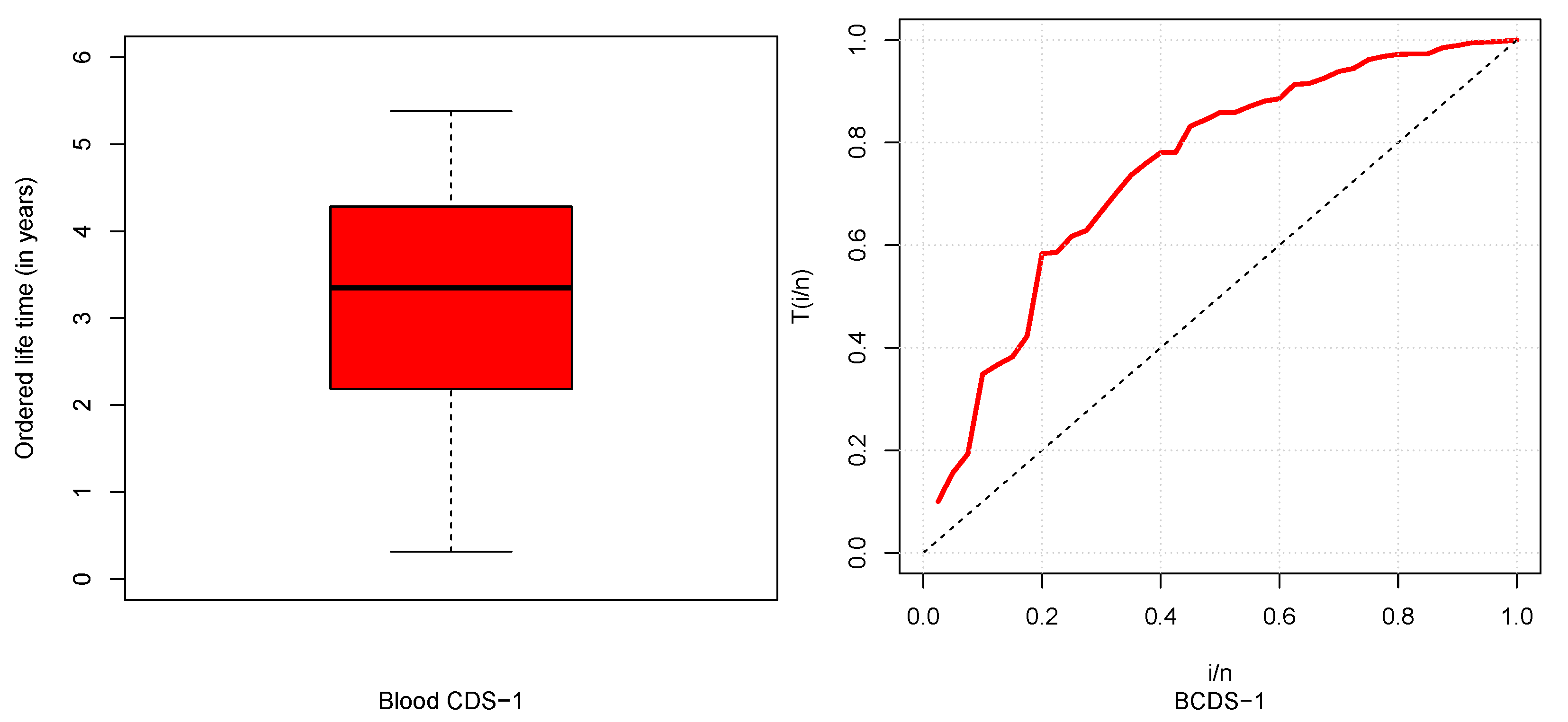
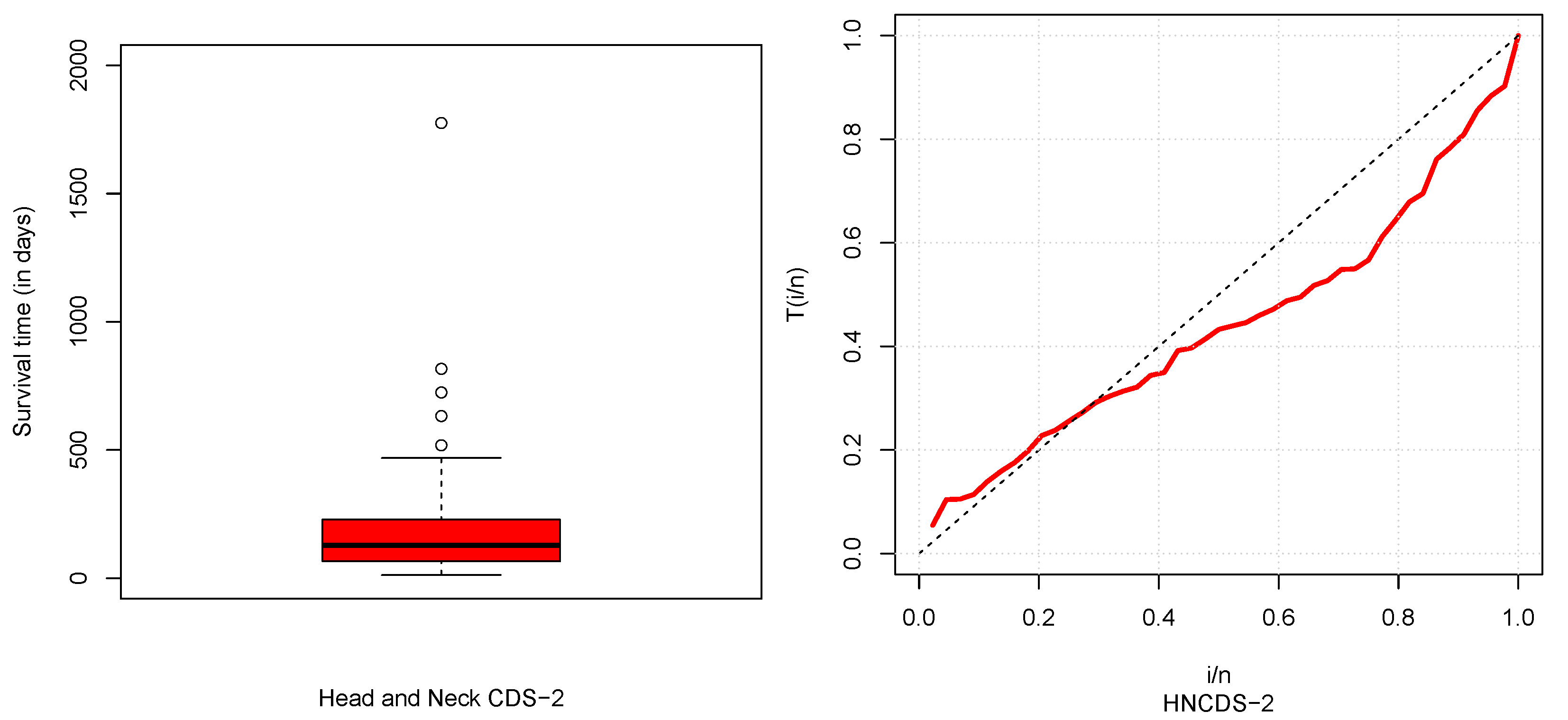
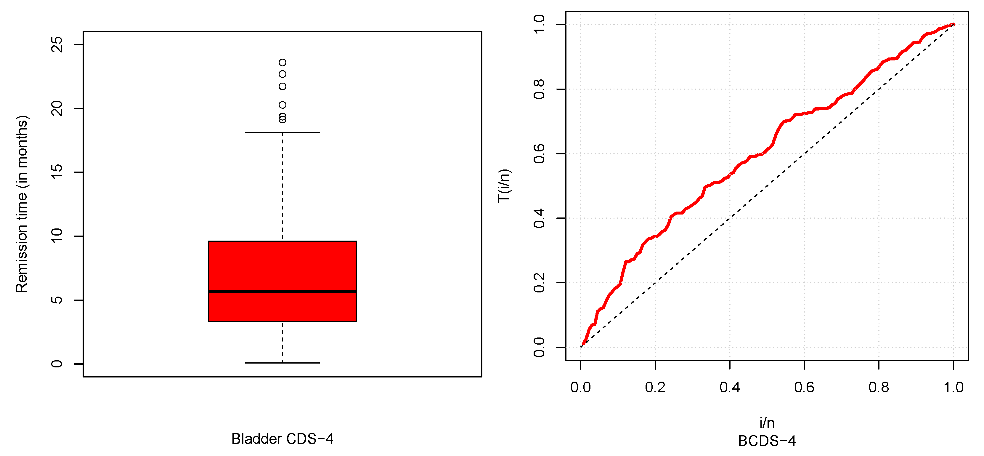
The descriptive statistics of CDSs are described in Table 5 and box and TTT plots are displayed in Figure 6, Figure 7, Figure 8 and Figure 9. From Table 5, it could be observed that HNCDS-2 and ABCDS-3 are right-skewed with high coefficients of kurtosis, while BCDS-1 is left-skewed. In Figure 7 and Figure 8, box plots indicate that HNCDS-2 and ABCDS-3 have extreme vales statistical behavior. Thus, these are suitable for distributions of extreme values and skewed models.

Table 5. Descriptive statistics for CDSs.

Data	BCDS-1	HNCDS-2	ABCDS-3	BCDS-4
n	40	44	73	132
Min.	0.3150	12.20	0.090	0.080
Ist Qu.	2.1990	67.21	0.920	3.348
Median	3.3480	128.50	1.570	5.665
3rd Qu.	4.2640	219.00	2.750	9.537
Mean	3.1407	223.48	3.755	7.149
Max.	5.3810	1776.00	86.010	23.600
Variance	1.8465	93286.41	112.331	27.673
Skewness	−0.4167	3.3838	6.799	1.072
Kurtosis	−0.7262	13.5596	48.777	0.669

Figure 6. Boxplot (left) and TTT plot (right) for BCDS-1.

Figure 7. Boxplot (left) and TTT plot (right) for HNCDS-2.

Figure 8. Boxplot (left) and TTT plot (right) for ABCDS-3.

Figure 9. Boxplot (left) and TTT plot (right) for BCDS-4.

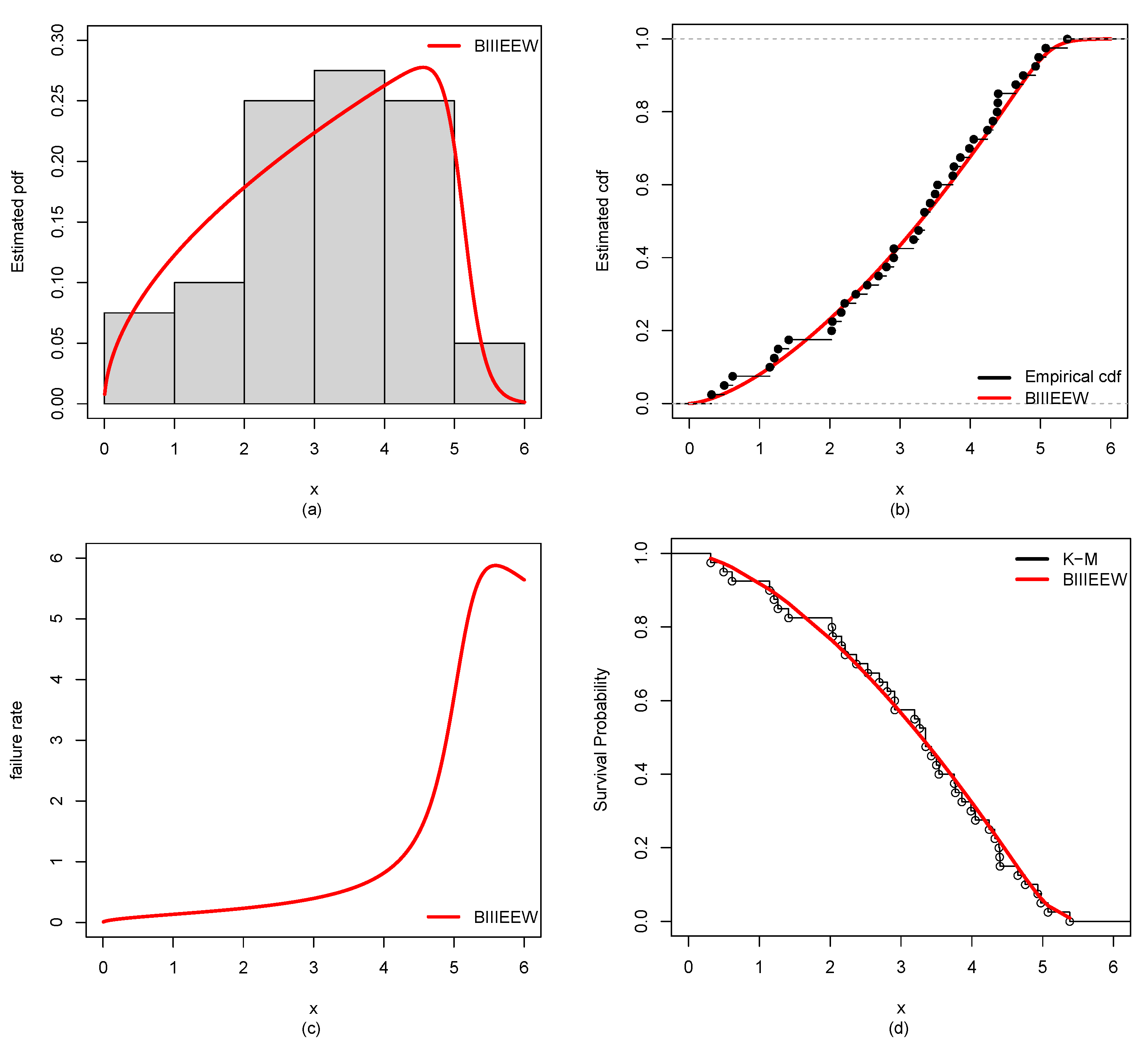
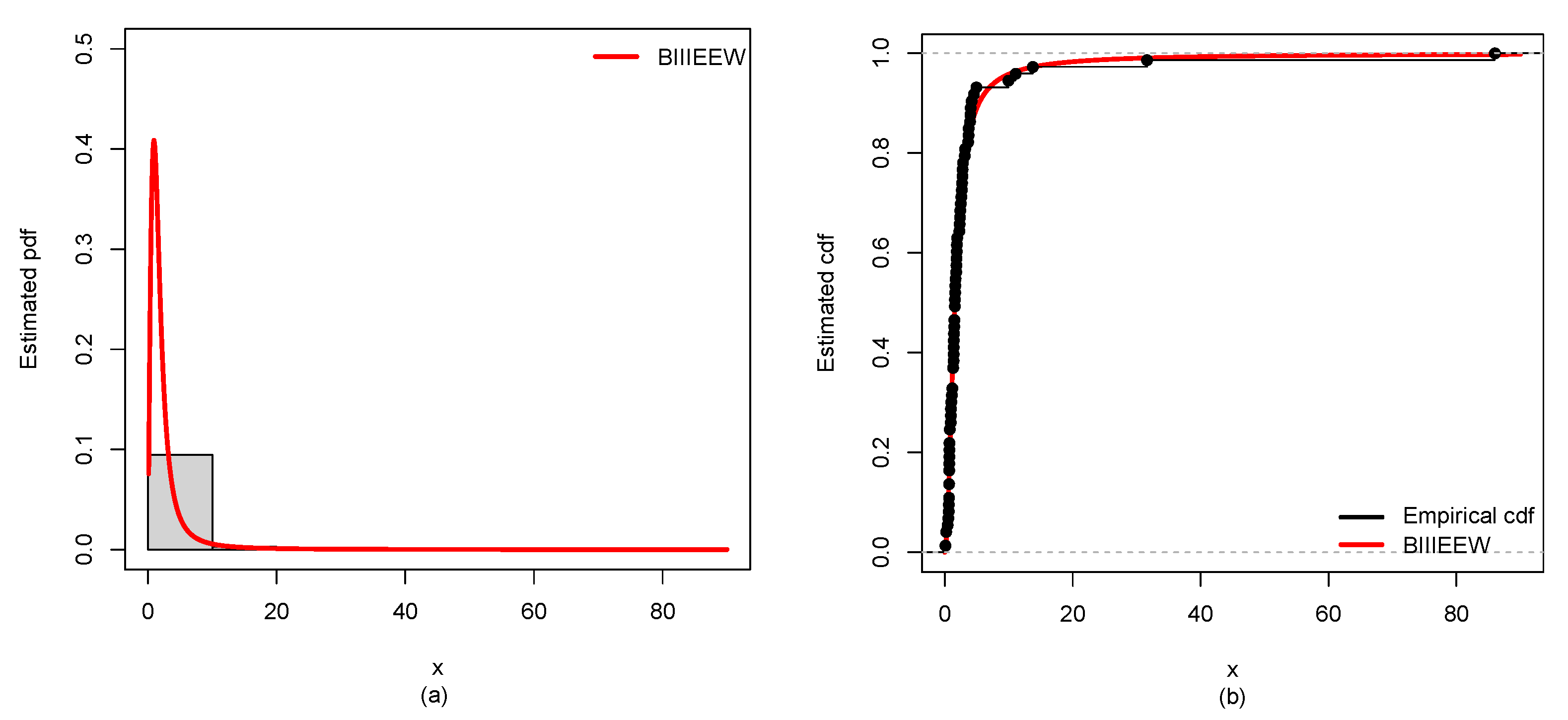
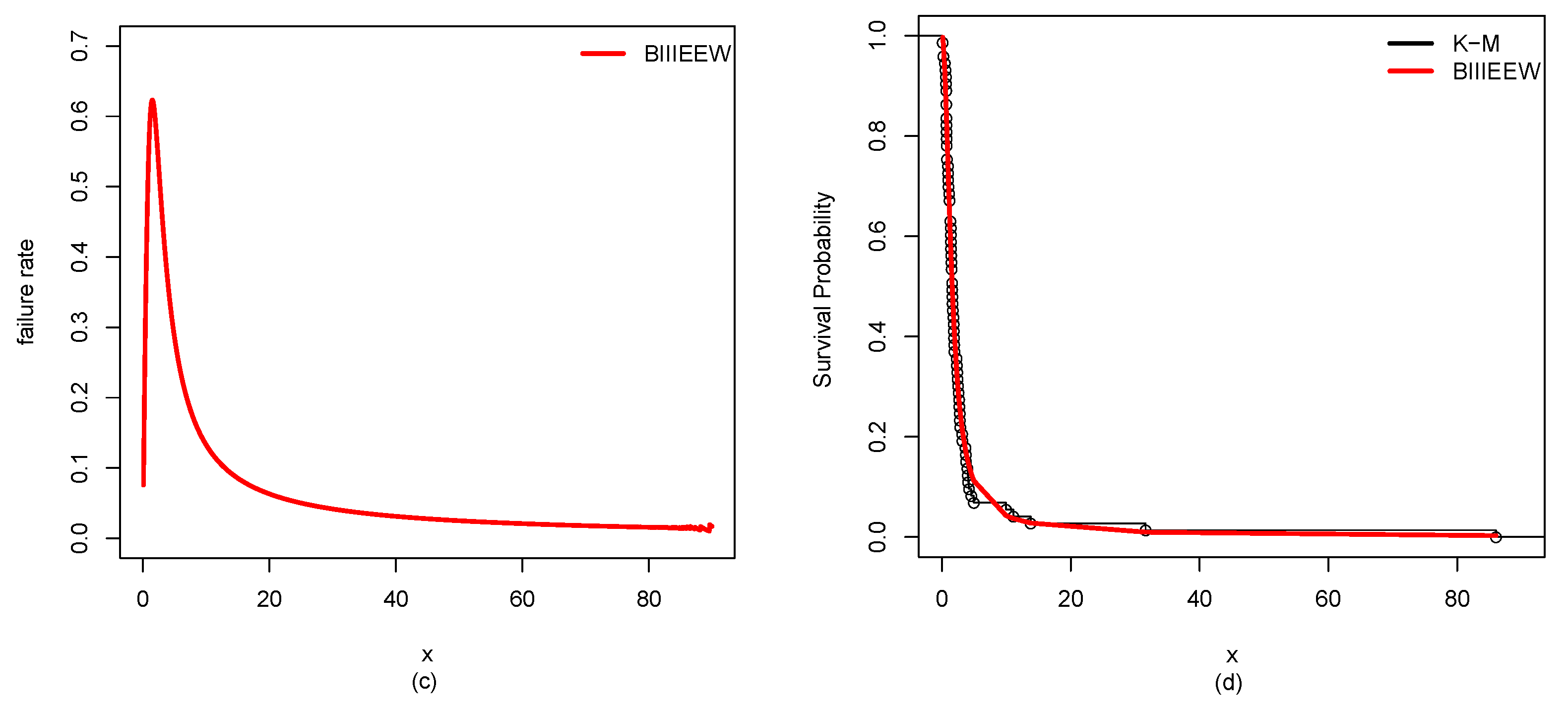
Furthermore, the results of ML estimates with corresponding SEs of the proposed BIIIEEWD in contrast of the other competing models for CDSs are provided in Table 6, Table 7, Table 8 and Table 9. The considered GoF measures values for CDSs of all candidate models are displayed in Table 10, Table 11, Table 12 and Table 13. From Table 10, Table 11, Table 12 and Table 13, it could be observed that the BIIIEEWD posses the smallest $-\widehat{L}$, $W^{*}$, $A^{*}$, AIC, BIC, and KS values for CDSs. In addition, it has the highest p-value at KS statistics against all fitted competing models. These results suggest that all fitted competing models fit quite well, but the proposed BIIIEEW model provides the best fit. Furthermore, Figure 10, Figure 11, Figure 12 and Figure 13 support these results for CDSs.

Table 6. ML estimates and SEs of parameters of the BIIIEEW model for BCDS-1.

Model	$\widehat{\mathit{\theta }}$	$\widehat{\mathit{c}}$	$\widehat{\mathit{k}}$	$\widehat{\mathit{\beta }}$	$\widehat{\mathit{\gamma }}$
BIIIEEW	0.71982	13.03392	0.04603	6.82169	3.55227
	(1.44108)	(41.79737)	(0.05557)	(7.47865)	(10.36960)
GOBPW	2.84630	3.21940	0.78820	1.45460	5.64530
	(0.17340)	(0.21990)	(0.10240)	(0.11350)	(2.47530)
GmLLW	4.95640	3.14070	1.34130	2.70340	7.94530
	(1.73540)	(0.21210)	(0.15050)	(0.20350)	(3.74620)
GmGMoW	3.25390	2.50030	3.51830	1.39260	5.65720
	(0.28450)	(0.33780)	(0.23160)	(0.07450)	(0.54930)
BMoW	2.64510	3.06980	3.01170	0.87210	4.87210
	(0.17340)	(0.41920)	(0.26480)	(0.06450)	(0.53910)
KmMoW	2.18350	3.46460	1.10320	1.74290	4.08320
	(0.63190)	(0.74040)	(0.25300)	(0.14390)	(1.35410)
BeLLW	1.94530	0.99320	0.64630	0.84530	2.62930
	(0.43520)	(0.10210)	(0.07260)	(0.09360)	(0.74530)

Table 7. ML estimates and SEs of parameters of the BIIIEEW model for HNCDS-2.

Model	$\widehat{\mathit{\theta }}$	$\widehat{\mathit{c}}$	$\widehat{\mathit{k}}$	$\widehat{\mathit{\beta }}$	$\widehat{\mathit{\gamma }}$
BIIIEEW	3.31393	12.26944	1.20636	0.49548	0.07396
	(5.22705)	(20.01934)	(0.88527)	(4.85634)	(0.08751)
GOBPW	5.25670	1.69090	25.03780	1.70180	3.44340
	(2.67430)	(0.21280)	(9.39440)	(1.18230)	(0.42360)
GmLLW	0.25630	4.84690	1.04080	3.45630	5.22080
	(0.13240)	(0.15690)	(0.11090)	(0.53410)	(2.97440)
KmMoW	1.35460	1.02340	0.45780	4.10360	2.97430
	(0.64540)	(0.18270)	(0.09910)	(1.03430)	(0.45830)
GmGMoW	8.34520	16.35720	6.72470	3.24360	18.25460
	(3.25430)	(4.74430)	(2.86690)	(1.01240)	(7.45320)
BeLLW	5.73520	51.17830	29.70710	4.83220	17.63240
	(2.11530)	(17.43520)	(8.84320)	(1.87430)	(6.53620)
BMoW	7.87320	37.52430	23.47700	5.53250	11.63490
	(2.65230)	(9.32450)	(6.96340)	(2.53420)	(3.64530)

Table 8. ML estimates and SEs of parameters of the BIIIEEW model for ABCDS-3.

Model	$\widehat{\mathit{\theta }}$	$\widehat{\mathit{c}}$	$\widehat{\mathit{k}}$	$\widehat{\mathit{\beta }}$	$\widehat{\mathit{\gamma }}$
BIIIEEW	2.84755	1.46752	0.57065	1.63629	0.89759
	(1.04539)	(0.24194)	(0.22568)	(0.00470)	( 0.00604)
GOBPW	1.74130	1.86900	1.61630	0.07310	1.98330
	(0.41310)	(0.18540)	(0.17250)	(0.00410)	(0.20230)
GmGMoW	0.09730	0.51960	1.03820	3.34570	0.56530
	(0.03670)	(0.12150)	(0.08590)	(1.95850)	(0.32010)
KmMoW	1.07040	1.11740	1.12800	2.70690	2.72850
	(0.21560)	(0.16440)	(0.20770)	(0.87170)	(1.19810)
GmLLW	0.38220	1.43420	0.71830	3.22470	0.37880
	(0.02530)	(0.12690)	(0.11490)	(0.60070)	(0.05830)
BeLLW	0.45670	2.11170	2.22080	7.53210	2.46790
	(0.83540)	(0.39510)	(0.24430)	(1.45670)	(0.55430)
BMoW	2.67490	3.75520	10.52570	3.35480	11.67360
	(1.53670)	(1.23190)	(0.87110)	(0.35470)	(3.57690)

Table 9. ML estimates and SEs of parameters of the BIIIEEW model for BCDS-4.

Model	$\widehat{\mathit{\theta }}$	$\widehat{\mathit{c}}$	$\widehat{\mathit{k}}$	$\widehat{\mathit{\beta }}$	$\widehat{\mathit{\gamma }}$
BIIIEEW	0.17521	1.86501	0.70097	17.38124	5.75015
	(0.05814)	(0.21181)	(0.29749)	(0.04119)	(0.04196)
GOBPW	3.01740	1.36900	7.81080	1.87480	5.92240
	(2.77700)	(0.09330)	(0.52260)	(0.25370)	(1.57770)
GmLLW	2.64730	1.63370	0.22850	1.60030	8.38840
	(0.40250)	(0.18420)	(0.03010)	(2.2953)	(3.65110)
GmGMoW	3.19930	1.97010	5.57350	1.42430	2.10570
	(0.70510)	(0.14390)	(0.42470)	(0.54220)	(0.23630)
BMoW	3.75310	6.51460	2.87810	0.93560	4.37650
	(0.34210)	(0.43480)	(0.21070)	(0.21320)	(0.63420)
KmMoW	5.38450	7.14820	5.24050	2.41150	2.10470
	(1.27530)	(0.45610)	(0.32250)	(1.19250)	(0.38850)
BeLLW	1.21220	5.41600	2.75570	1.35640	5.38260
	(0.10930)	(0.39990)	(0.30860)	(0.04320)	(0.68030)

Table 10. GoF measures for the BIIIEEW model for BCDS-1.

Model	$-\widehat{\mathit{L}}$	${\mathit{W}}^{*}$	${\mathit{A}}^{*}$	AIC	BIC	KS	p-Value
BIIIEEW	65.102	0.02195	0.14759	140.204	148.648	0.06610	0.9948
GOBPW	68.510	0.04800	0.42240	147.020	155.464	0.08300	0.9158
GmLLW	69.590	0.06370	0.44720	149.180	157.624	0.09020	0.8651
GmGMoW	70.150	0.11660	0.85640	150.300	158.744	0.11840	0.7316
BMoW	73.390	0.17660	1.54490	156.780	165.224	0.14410	0.5967
KmMoW	76.540	0.25180	1.55700	163.080	171.524	0.15820	0.3480
BeLLW	79.020	0.39830	2.33600	168.040	176.484	0.17710	0.1478

Table 11. GoF measures for the BIIIEEW model for HNCDS-2.

Model	$-\widehat{\mathit{L}}$	${\mathit{W}}^{*}$	${\mathit{A}}^{*}$	AIC	BIC	KS	p-Value
BIIIEEW	277.703	0.01317	0.10698	565.407	574.328	0.04582	0.9999
GOBPW	277.790	0.01370	0.11640	565.580	574.501	0.04960	0.8438
GmLLW	277.460	0.02180	0.14030	564.920	573.841	0.06840	0.7231
KmMoW	282.010	0.18440	0.98610	574.020	582.941	0.14720	0.6381
GmGMoW	289.390	0.39380	2.69420	588.780	597.701	0.18820	0.3081
BeLLW	302.910	0.44640	3.08110	615.820	624.741	0.21800	0.1721
BMoW	313.680	0.95740	5.04830	637.360	646.281	0.26910	0.0240

Table 12. GoF measures for the BIIIEEW model for ABCDS-3.

Model	$-\widehat{\mathit{L}}$	${\mathit{W}}^{*}$	${\mathit{A}}^{*}$	AIC	BIC	KS	p-Value
BIIIEEW	138.527	0.04848	0.37429	287.054	298.507	0.07352	0.8249
GOBPW	139.980	0.05240	0.46870	289.960	301.412	0.06730	0.5127
GmGMoW	144.260	0.16490	1.16500	298.520	309.972	0.09430	0.4821
KmMoW	147.900	0.29190	1.84080	305.800	317.252	0.14110	0.2386
GmLLW	153.290	0.53020	3.58210	316.580	328.032	0.15890	0.1359
BeLLW	221.360	1.61760	3.75730	452.720	464.172	0.28690	0.0731
BMoW	275.410	3.74270	8.34280	560.820	572.272	0.38810	0.0176

Table 13. GoF measures for the BIIIEEW model for BCDS-4.

Model	$-\widehat{\mathit{L}}$	${\mathit{W}}^{*}$	${\mathit{A}}^{*}$	AIC	BIC	KS	p-Value
BIIIEEW	382.021	0.03002	0.17785	774.042	788.456	0.04014	0.9835
GOBPW	382.530	0.03370	0.20870	775.060	789.474	0.04430	0.7146
GmLLW	383.310	0.03680	0.24550	776.620	791.034	0.05090	0.6732
GmGMoW	391.060	0.07640	0.89330	792.120	806.534	0.06770	0.3401
BMoW	404.120	0.26400	2.45860	818.240	832.654	0.09650	0.2721
KmMoW	405.940	0.56550	3.45940	821.880	836.294	0.12780	0.1397
BeLLW	418.340	0.59810	4.32780	846.680	861.094	0.15170	0.1259

Figure 10. Plots of the estimated (a) PDF using a histogram, (b) CDF using empirical CDF, (c) failure rate, (d) Kaplan–Meier (K-M) survival probability of BIIIEEWD for BCDS-1.

Figure 11. Plots of the estimated (a) PDF using a histogram, (b) CDF using empirical CDF, (c) failure rate, (d) K-M survival probability of BIIIEEWD for HNCDS-2.

Figure 12. Plots of the estimated (a) PDF using a histogram, (b) CDF using empirical CDF, (c) failure rate, (d) K-M survival probability of BIIIEEWD for ABCDS-3.

Figure 13. Plots of the estimated (a) PDF using a histogram, (b) CDF using empirical CDF, (c) failure rate, (d) K-M survival probability of BIIIEEWD for BCDS-4.

7. Conclusions

The field of medical research relies heavily on applications of statistical distributions, where applications have the potential to significantly improve public health, particularly for cancer patients. In this article, therefore, the WEE-X, LEE-X, LGCEE-X, and BIIIEE-X families have been proposed as new families of continuous distributions. Four new models, i.e., WEEW, LEEW, LGCEEW, and BIIIEEW, are derived and explored graphically. In this regard, we characterized the BIIIEE-X family with a five-parameter model, i.e., BIIIEE-Weibull. Various properties of the proposed model have also been derived. Consequently, the proposed model is applied to four distinct cancer data, including bladder, acute bone, neck and head, and blood. GoF measures have been compared with other competing models to see how well the proposed BIIIEEW model performed. Our proposed model have shown superior graphical and numerical results. When it comes to modeling positively skewed lifetime data, particularly cancer research, we hoped that our proposed model would serve as a better alternative to other more conventional distributions.

Using a Bayesian approach, the parameters of the various models derived from these proposed families can be estimated in future work. Besides, other datasets in various regions can be utilized to actually take a look at the adaptability of the determined models. For the bivariate families of distributions, this work can also be extended. Some other flexible distributions should also be considered besides the distribution proposed in this study to fit the data of the real-life case studies.

References

- Jose, K.K.; Naik, S.R. On the q-Weibull Distribution and Its Applications. Commun. Stat.-Theory Methods 2009, 38, 912–926. [Google Scholar] [CrossRef]
- Baghestani, A.R.; Moamer, S.; Pourhoseingholi, M.A.; Khadem Maboudi, A.A.; Ghoreshi, B.; Zali, M.R. Demographic and Pathological Predictors of Colorectal Cancer Survival in Competing Risk Model, Using Generalized Weibull Distribution, (in en). Int. J. Cancer Manag. 2017, 10, e7352. [Google Scholar] [CrossRef]
- Idowu, B.; Ikegwu, E.M. The Beta Weighted Weibull Distribution: Some Properties and Application to Bladder Cancer Data. J. Appl. Comput. Math. 2013, 2, 1–6. [Google Scholar] [CrossRef]
- Yousof, H.M.; Afify, A.Z.; Cordeiro, G.M.; Alzaatreh, A.; Ahsanullah, M. A new four-parameter Weibull model for lifetime data. J. Stat. Theory Appl. 2017, 16, 448–466. [Google Scholar] [CrossRef]
- Elgohari, H.; Yousof, H. New extension of weibull distribution: Copula, mathematical properties and data modeling. Stat. Optim. Inf. Comput. 2020, 8, 972–993. [Google Scholar] [CrossRef]
- Afify, A.Z.; Kumar, D.; Elbatal, I. Marshall-Olkin power generalized Weibull distribution with applications in engineering and medicine. J. Stat. Theory Appl. 2020, 19, 223–237. [Google Scholar] [CrossRef]
- Ijaz, M.; Asim, S.M.; Farooq, M.; Khan, S.A.; Manzoor, S. A Gull Alpha Power Weibull distribution with applications to real and simulated data. PLoS ONE 2020, 15, e0233080. [Google Scholar] [CrossRef] [PubMed]
- Alzaatreh, A.; Famoye, F.; Lee, C. A new method for generating families of continious distributions. Metron 2013, 71, 63–79. [Google Scholar] [CrossRef]
- Tahir, M.H.; Cordeiro, G.M. Compounding of distributions: A servey and new generalized classes. J. Stat. Distrib. Appl. 2016, 3, 13. [Google Scholar] [CrossRef]
- Hussain, S.; Rashid, M.S.; Ul Hassan, M.; Ahmed, R. The Generalized Alpha Exponent Power Family of Distributions: Properties and Applications. Mathematics 2022, 10, 1421. [Google Scholar] [CrossRef]
- Flajonet, P.; Odlyzko, A. Singularity analysis of generating function. SIAMJ. Discr. Math. 1990, 3, 216–240. [Google Scholar] [CrossRef]
- Flajonet, P.; Sedgewich, R. Analytic Combinatorics; Cambridge University Press: Cambridge, UK, 2009; ISBN 978-0-521-89806-5. [Google Scholar]
- Hussain, S.; Sajid Rashiid, M.; Ul Hassan, M.; Ahmed, R. The Generalized Exponential Extended Exponentiated Family of Distributions: Theory, Properties, and Applications. Mathematics 2022, 10, 3419. [Google Scholar] [CrossRef]
- Hussain, S.; Ul Hassan, M.; Sajid Rashiid, M.; Ahmed, R. The Exponentiated Power Alpha Index Generalized Family of Distributions: Properties and Applications. Mathematics 2023, 11, 900. [Google Scholar] [CrossRef]
- Kenney, J.; Keeping, E. Mathematics of Statistics, 3rd ed.; D. Van Nostrand: Princeton, NJ, USA, 1962; Volume 1. [Google Scholar]
- Moors, J.J.A. A quantile alternative for kurtosis. Statistician 1998, 37, 25–32. [Google Scholar] [CrossRef]
- Suleiman, A.A.; Othman, M.; Ishaq, A.I.; Abdullah, M.L.; Indawati, R.; Daud, H.; Sokkalingam, R. A New Statistical Model Based on the Novel Generalized Odd Beta Prime Family of Continuous Probability Distributions with Applications to Cancer Disease Data Sets. Comput. Sci. Math. 2022. [Google Scholar] [CrossRef]
- Foya, S.; Oluyede, B.O.; Fagbamigbe, A.F.; Makubate, B. The gamma log-logistic Weibull distribution: Model, properties, and application. Electron. J. Appl. Stat. Anal. 2017, 10, 206–241. [Google Scholar] [CrossRef]
- Oluyede, B.O.; Huang, S.; Yang, T. A new class of generalized modified weibull distribution with applications. Austrian J. Stat. 2015, 44, 45–68. [Google Scholar] [CrossRef]
- Silva, G.O.; Ortega, E.M.M.; Cordeiro, G.M. The beta modified Weibull distribution. Lifetime Data Anal. 2010, 16, 409–430. [Google Scholar] [CrossRef] [PubMed]
- Cordeiro, G.M.; Ortega, E.M.M.; Silva, G.O. The Kumaraswamy modified Weibull distribution: Theory and applications. J. Stat. Comput. Simul. 2012, 84, 1–25. [Google Scholar] [CrossRef]
- Makubate, B.; Oluyede, B.O.; Dingalo, N.; Fagbamigbe, A.F. The Beta Log-Logistic Weibull Distribution: Model, Properties and Application. Int. J. Stat. Probab. 2018, 7, 49–67. [Google Scholar] [CrossRef]
- Al-Saiary, Z.A.; Bakoban, R.A. The Topp-Leone generalized inverted exponential distribution with real data applications. Entropy 2020, 22, 1144. [Google Scholar] [CrossRef] [PubMed]
- Ibrahim, S.; Doguwa, S.I.; Isah, A.; Haruna, J.M. The Topp Leone Kumaraswamy-G Family of Distributions with Applications to Cancer Disease Data. J. Biostat. Epidemiol. 2020, 6, 40–51. [Google Scholar]
- Mansour, M.M.; Yousof, H.M.; Shehata, W.A.M.; Ibrahim, M. A new two parameter Burr XII distribution: Properties, copula, different estimation methods and modeling acute bone cancer data. J. Nonlinear Sci. Appl. 2020, 13, 223–238. [Google Scholar] [CrossRef]
- Varghese, J.; Jose, K.K. Kumaraswamy harris generalized kumaraswamy distribution and its Application in Survival Analysis. Biom. Biostat. Int. J. 2022, 11, 28–34. [Google Scholar]
Disclaimer/Publisher’s Note: The statements, opinions and data contained in all publications are solely those of the individual author(s) and contributor(s) and not of MDPI and/or the editor(s). MDPI and/or the editor(s) disclaim responsibility for any injury to people or property resulting from any ideas, methods, instructions or products referred to in the content. |
© 2023 by the authors. Licensee MDPI, Basel, Switzerland. This article is an open access article distributed under the terms and conditions of the Creative Commons Attribution (CC BY) license (https://creativecommons.org/licenses/by/4.0/).