1. Introduction
IP traffic model development is an important research field in the context of network technologies that can be applied to the Internet or, more generally, to any communication network. The significance of these models can be divided into the following two groups: First, IP traffic models are needed as input into network simulations. These simulations must be performed in order to study and validate network algorithms and protocols which will be applied to real traffic and in order to analyze how IP traffic responds to the occurrence of different conditions and network situations, for example network overload or other exceptional situations. It is therefore important that the proposed models reflect the relevant network traffic operating characteristics as closely as possible. Second, a well-designed model can help one to better understand the characteristics of the network traffic, an understanding which could also be helpful during the design process of routers and other devices that control network traffic.
In the field of mathematical modeling of IP networks, two-state, Markov-modulated On–Off processes (MMP) represent an important group of models. In a relatively simple way, by changing their parameters, they can model different important types of IP flows, from a Bernoulli flow, which is suitable for modeling the aggregation of several services, to a “regular flow” and to a flow with significant On–Off periods, which is used, for example, in VoIP transmission modeling. When modeling two-state network nodes, using the MMP process as an arrival flow model enables the construction of a relatively simple Markov queuing system.
In the context of sizing single-server queuing systems, two-state MMP processes take on the analytical form “effective bandwidth” (scale-cumulant generative function). This fact makes it possible to use two-state MMP processes when sizing network devices.
For example, n-state MMPs () provide better options for modeling IP flows, but they only have a numerical calculation of EB. Another group consists of, e.g., self-similar processes, but with them, EB often does not even exist. Use of the mentioned processes as models of IP flows for the overall dimensioning of IP devices leads to the construction of complicated models of queuing systems.
This paper deals with two types of two-state, Markov-modulated On–Off processes, assuming a discrete time with given time slots. The first type represents a two-state Markov chain which in the state (on period) generates 1 and in the state (Off period) generates 0 or silence. We will refer to this stochastic process as MMRP (Markov-modulated regular process). The second type is a two-state Markov chain which in the state (On period) generates a Bernoulli process with intensity p. We will refer to this process as MMBP (Markov-modulated Bernoulli process). During our study, we performed an analysis of the probabilistic characteristics of these processes, and based on the acquired knowledge, we created a method for estimating unknown parameters from the measured IP traffic.
The MMRP process has only two parameters, and , which represent the probabilities of transitions between the On and Off states. For their estimation, we used data on the average rate of packets in the monitored time window of the monitored IP traffic and the peak rate fluctuations probability shape.
In addition to the and parameters, the MMBP process also has the Bernoulli process parameter p. Since we were able to derive the moments of a random variable that describes the gaps between packets in this process, we also obtained a method of estimating unknown parameters with measured IP traffic.
The advantage of modeling IP flows using two-state Markov-modulated processes is that, for these processes, the analytical expression of effective bandwidth is known. This allows us to very easily and quickly dimension the necessary network interfaces for the transmission of monitored IP traffic with respect to QoS parameters, maximum delay, and probability packets lost.
2. Related Work
In general, the Markov-modulated Bernoulli process (MMBP) represents a Markov process with a countable set of states
. If the chain is in state
, then the system starts generating Bernoulli flow with intensity
. Such a model is described, for example, in Reference [
1], where transient analysis and Ergodic analysis are also found. In References [
2,
3], in addition to the basic description, they also deal with the influence of the MMB arrival process on the RED-like active queue management algorithm. In Reference [
4], they deal with the basic analysis of the MMBP process, introduce a general generation function for inter-arrival time, and analyze the behavior of the queue at the MMBP input. In Reference [
5], we find the Bayesian analysis of the MMBP process. Transient analysis of the queuing system MMBP/D/1/K queue is described in Reference [
6]. In Reference [
7], the Markov-modulated Bernoulli process model is used to analyze the delay experienced by messages in clocked, packed-switched Banyan networks with
output-buffered switches. In Reference [
8], when modeling bursty and correlated traffics, the authors use the two-state Markov-modulated Bernoulli arrival process. In Reference [
9] four-dimensional, discrete-time Markov chain development is described and used for the performance analysis of leaky bucket algorithms.
The article in Reference [
10] deals with ATM networks supporting B-ISDN. Authors use the two-state Markov-modulated Bernoulli process as a model output process from the queuing system D-BMAP/D/1/K.
In article [
11], we can find usage of Markov chains and hidden Markov models used for mobile application network traffic modelling. Several articles, for example, Reference [
12], investigate the QoS parameters, the mean waiting time, and the probability of packet loss in a single-server finite queuing system with exponential service, which includes a self-similar arrival process emulated by a circulant Markov-modulated Poisson process (system CMMPP/M/1/K).
Finite-state Markov modeling was also used for reliability prediction of this typical industrial wireless network [
13].
Another usage of Markov models was proposed in Reference [
14]. The authors propose a hybrid Markov model (HMM) for the performance analysis of connection provisioning with guaranteed availability in WDM optical networks.
A novel usage of Markov modelling, multivariate multi-order Markov transition to realize multi-modal accurate predictions was proposed in Reference [
15].
3. Basic IP Flow Description
The basic elements of an IP network are network devices (nodes) and packet flows. Packet flows can be described in several ways. For example, a deterministic model of the IP network (Network Calculus) uses subadditive curves to describe IP flows. In the stochastic model, effective bandwidth is usually used to describe flows.
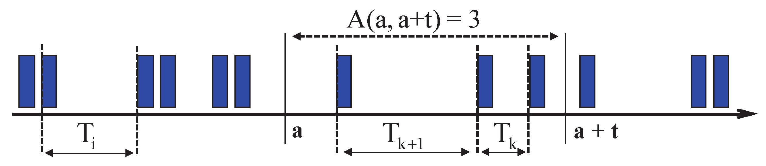
Overall, there are two basic procedures for describing and analyzing IP flows. The first is with the aid of the above process
, which describes the number of occurrences of packets in the interval
. The second way is through analysis of the probability distributions of random variables
, which describe the gaps between the occurrence of individual packets. An example of both methods is shown in
Figure 1:
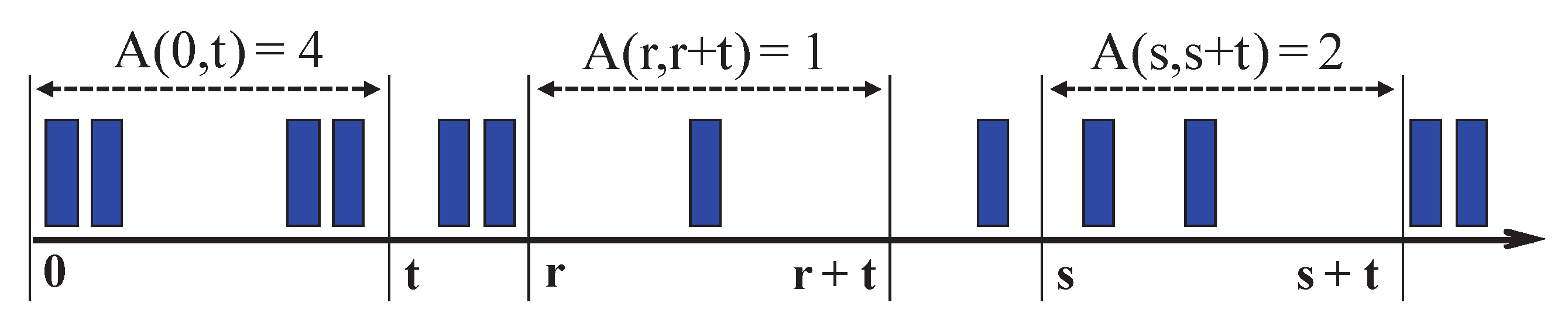
Using the stochastic model of the IP network, we assume that represents a cumulative stochastic process and are undeniably random variables. Another simplification of the model is that we assume represents a stationary random process. This means that all probabilistic characteristics of the sequence are invariant due to the time. Simply put, it does not matter at which point in time we observe the flow, only the length of the observations matters.
Thanks to this time invariance property, we can introduce the random process
, which describes the number of occurrences of packets in an arbitrary interval of length
t:
Thanks to the time invariance of the stationary random process
, the non-negative random variables
, which describe the gaps between the occurrence of packets in the flow, have the same probability distribution. Therefore, from now on we will describe the gaps in the stationary process with one random variable,
T, which has a distribution function
,
.
Figure 2 displays stationary flow:
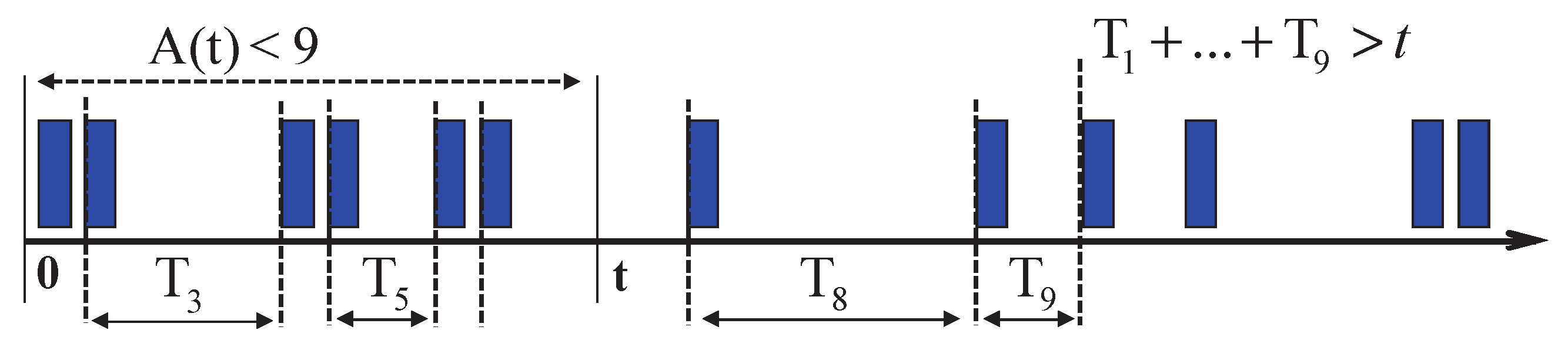
Between the probability distributions of the stationary process
and random variables
, the following relation applies: If less than
k events occur in the stream during time
t, then the sum of the first
k gaps is greater than the time
t. Therefore, the probabilities that the mentioned events will occur are equal.
Figure 3 displays the situation for
:
If the IP traffic is measured in given time slots, then the process
consists of the so-called increments
that record the occurrence of packets in time slots
i. No packet occurred at time zero; therefore,
:
If we consider a time window of length
n time slots, the basic characteristics of an IP flow, average rate
, and peak rate
have shape:
We denote the probability that
k packets occur in a time window of length
n:
4. Bernoulli Process
The simplest stochastic model of packet flow, or IP traffic, is represented by the Bernoulli process. It is defined by two properties: the occurrences of packets in the flow are independent of each other and the probability of packet occurrence in a time slot does not change over time. The time slot in which a maximum of one packet can occur is defined as an elementary slot.
For a better understanding of the Bernoulli process structure, we will show several simulations of the flow increments for the changing parameter
p. We can imagine the simulation as a flip of a coin, where the probability of getting a head is
p and the probability of getting a tail is
; see
Table 1:
Thus, the random process
will describe the occurrence of packets in
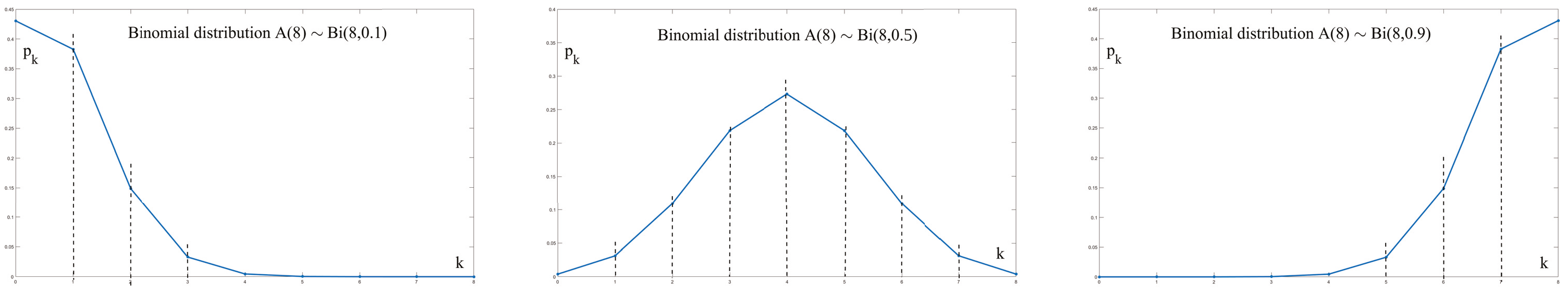
n elementary time slots. Due to independence, this process has a Binomial probability distribution:
The basic flow characteristics have the shape:
The probability distribution
for
and
is shown in
Figure 4:
A random variable
T which describes the size of the gap between packets has a geometric distribution,
:
The mean, variance, and coefficient of variation of the distribution have the shape:
If we have a detailed IP flow measurement available, e.g., from Wireshark, then we can very easily estimate
and
. Using the coefficient of variability
, we can decide whether it makes sense to deal with the Bernoulli process at all:
The parameter p represents the probability of the packet occurrence; therefore, if we obtain as a measurement, then it is not feasible to use the Bernoulli process for modeling.
Figure 5 shows the simulation of the Bernoulli process for different probabilities
p and different sampling increments
,
, and 8. We present the visualization of a variety of Bernoulli flows to allow for subsequent comparison with a variety of MMRP and MMBP processes in the following chapters.
In
Figure 5, for further clarification, a simulation of 200 increments
is shown, while the probability of the packet occurrence is set to
and
. We will also increase the values of increments
from 1 to 8.
In the first row of
Figure 5 we see how, with the gradually changing probability
p, we obtain first, when
, so-called “empty” flow with minimal occurrence of packets. After the probability increases to
, the fair “coin” flow is apparent, and with
, finally “bursty” flow is present. In the second row of
Figure 5, there are
processes sampled by two elementary slots. Furthermore, the third row contains an example of sampling by 8 elementary slots, which is defined by the process
. In all three examples, we see the course of events typical for stationary processes (with intensities
= 0.8 p/ts, 4 p/ts and 7.2 p/ts).
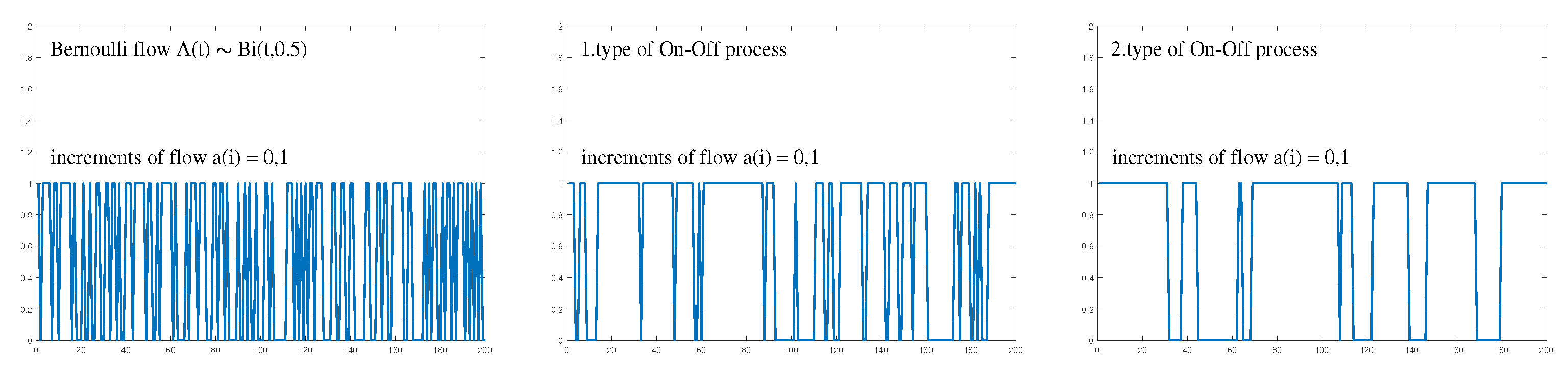
The Bernoulli process is a suitable model for IP flows in which a large number of IP services are aggregated (e.g., a core network). However, it cannot model flows in which there is significant alternation of On and Off periods, such as in VoIP and IPTV; see
Figure 6:
The Bernoulli process cannot model such significant transmission and silence periods as On–Off processes.
5. Markov-Modulated On–Off Regular Process
The Markov modulated On–Off regular process (MMRP) represents a two-state Markov chain with discrete time which, in the On state (
), generates a deterministic flow of IP traffic, and in the Off state (
), generates zeros, respectively, and does not broadcast any traffic. In the past, we have dealt with the basic analysis and usage of this process in IPTV traffic modeling in articles [
16,
17].
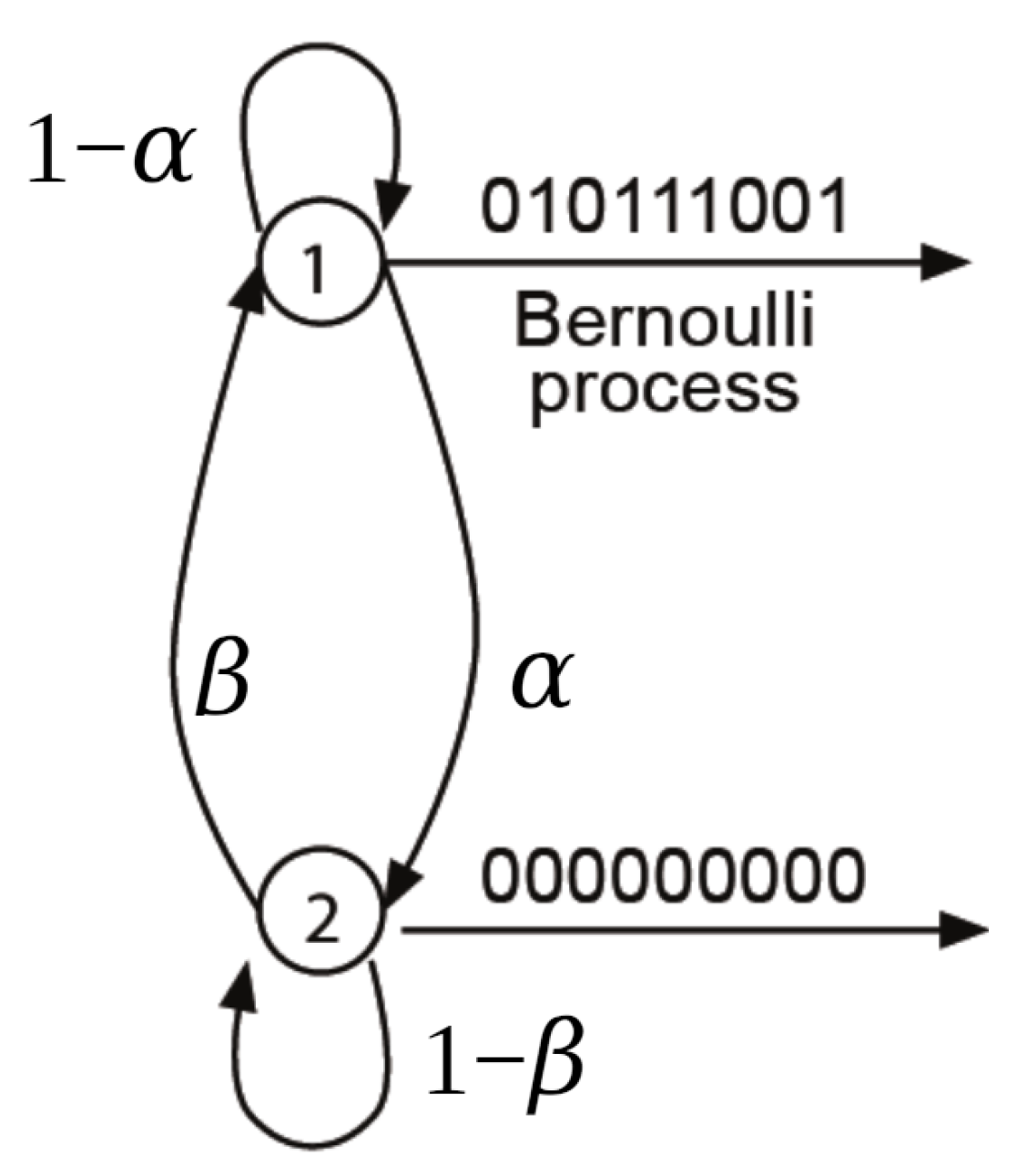
We denote by and the probabilities of transitions between states and in one time step . Modulation of the process is handled by a two-state Markov chain. Without prejudice to generality, we will assume that in the On state, the unit source (bits, packets, or frames) transmits at a constant speed of 1 [paket/ts].
The Markov chain is uniquely described by its set of states
and the matrix of transition probabilities
. We denote the steady-state probability distribution of a Markov chain by a vector
. We calculate it from the following system of linear equations:
A transition graph of the two-state Markov chain is shown in
Figure 7:
The simulation of the MMRP process is more complicated than it was with the Bernoulli process. Switching between the On and Off periods can be like tossing two coins,
-coin (probability of getting Head is
) and
-coin (probability of getting Head is
). If the chain switches to the On state, it will generate 1 with probability
; if it remains in the On state in the next time slot, it will generate 1 with probability
. A similar rule applies to generating 0. For comparison, we simulate the same 0/1 sequence as in the previous chapter in
Table 2:
We can model different types of IP flows by appropriate setting of and parameters. If the values are close to zero, , the chain minimally switches between states and therefore the flow contains significant On and Off periods, the so-called flow with bursty period. We get the opposite extreme if we set the parameter values close to one, . In that case, the flow switches almost constantly between 0 and 1, and we can speak of a deterministic flow. In case , the MMRP process turns into a Bernoulli process with parameter .
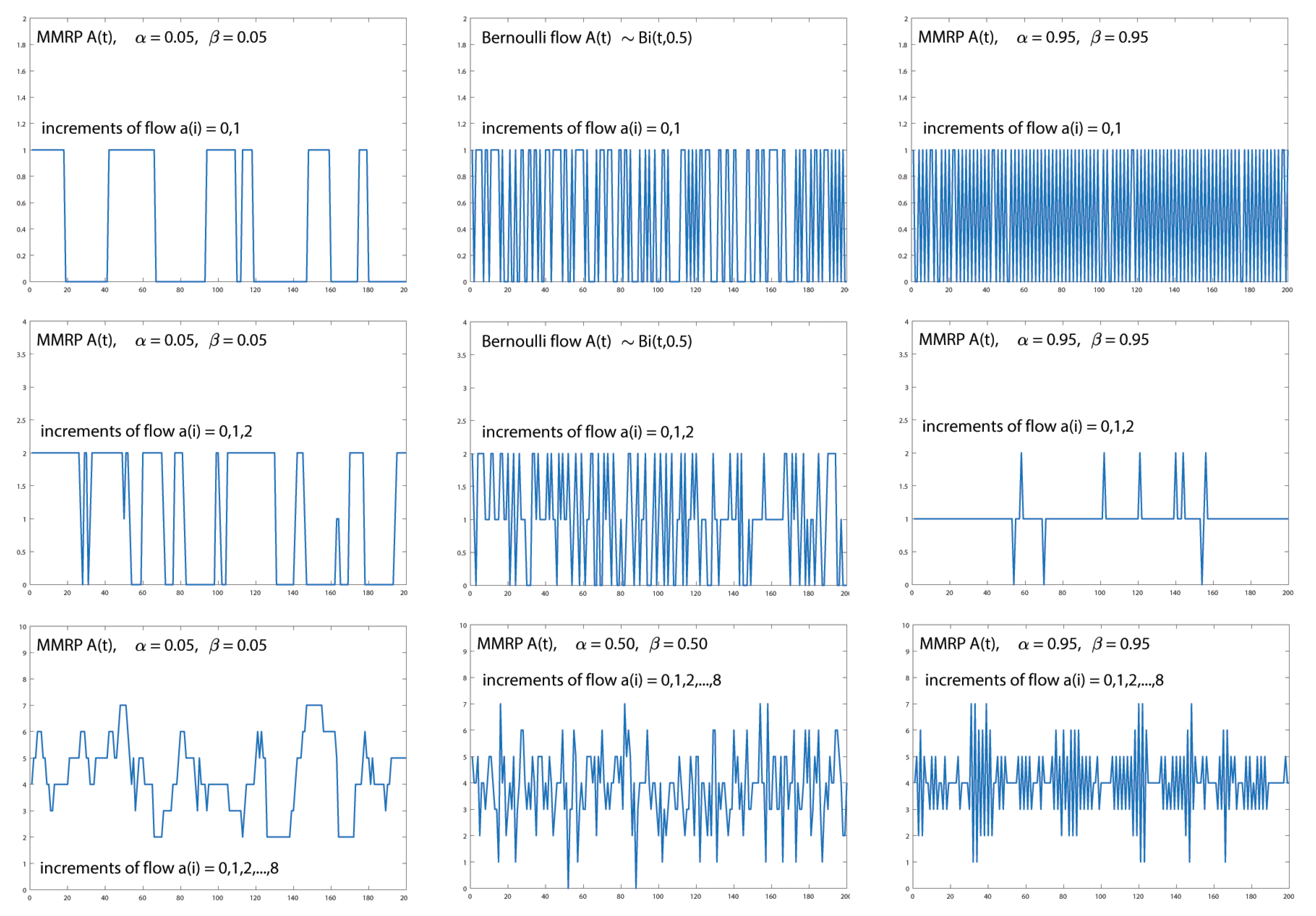
To clarify the situation, we will show a simulation of 200 increments
, while we will gradually set the switching probabilities between the states of the Markov chain to the values
, and
. The simulations are shown in
Figure 8.
In the first column of
Figure 8, there is a simulation of the On/Off process with
. On the 0/1 record, we see a marked alternation of the time when packets are sent and the gaps between the occurrence of packets. The second column is the process with parameters
. It is actually the same record of the Bernoulli flow that we already used in
Figure 5. In the third column is the simulation of the process with
. With such a setting, there is relatively fast switching between 0/1 generation. Looking at the course of the
process (2nd row, 3rd column), we can consider this process almost deterministic. In the third row is the record of the simulation of
processes. In all three cases, we see a significant difference in the internal structure of the processes, which is caused by a different correlation between the individual increments
.
5.1. Probability Distribution of MMRP
Using the complete probability theorem, we derive the distribution of the random process
or distribution of increments in one elemental slot:
We derived that the random process has an alternative probability distribution with moments and . According to the obtained results, we could say that the MMRP is no different from the Bernoulli process, just put and . However, we must realize that the MMRP process is governed by a two-state Markov chain, in which there is a dependency between two consecutive states. Therefore, analysis of the MMRP process only on the basis of the situation in elementary slots, or based on a 0/1 sequence, is misleading.
Using the complete probability theorem, we derive the distribution of the random process
, or the distribution of increments during two elemental slots.
We derive the characteristics of the random process
:
The form of the mean value is natural. However, the dispersion of has a different form from the Bernoulli process, and the dispersion of the packets occurrence also depends on the parameters and .
We derived probability distributions for random processes
and
in the articles [
16,
17]. For the process
, we have the form:
Probability distribution of a random process
:
Thanks to the knowledge of the distribution of increments in the
process, we can compare the probability of occurrence of the number of increments with the process
. We will compare processes with the same mean value of increments. In all of
Figure 9a–c, we have marked the probability distribution of the Bernoulli process when
with a blue line. Compared processes have the same mean values of increments, successively;
Figure 9a is
,
Figure 9b is
, and
Figure 9c is
:
In all of
Figure 9, we have marked the probability distribution for the Bernoulli process when
with a solid blue line. In
Figure 9b, an example of symmetric probability distributions,
. Thanks to the appropriate choice of parameters, the MMRP process can model a wide range of flows, from deterministic with a most-frequent occurrence of
, through the Bernoulli process
, to an On–Off process with the occurrence of mainly
and
. We notice that when
, we obtain a uniform distribution of increments. Similar variability of the distributions can also be observed in the asymmetric cases in the images
Figure 9a,c.
5.2. Probability Distribution of Time Spaces
We define the gap between the occurrence of packets in the MMRP process as a sequence of zeros (no packet occurred in the elementary slot), which will end the occurrence of the unit (packet). We describe the gaps between packets with the random variable
T. The gap starts by switching the source to the Off state, when the first zero is generated, then the count time slots in which the system remains in the Off state corresponds to the remaining length of the considered gap, and finally the gap ends by generating 1 by switching to the On period. A zero gap represents the occurrence of two consecutive packets. The random variable
T has the following probability distribution (see [
17] and
Figure 10):
We obtain the moments of the random variable
T using the moment-generating function (MGF)
:
Using the derivative of the MGF, we determine the first, second, and third initial moments:
We obtain the variance of the
T variable using second-order initial moments:
The coefficient of variability of gaps in the MMRP process has the form:
We obtain the third central moment
using the third orders of initial moments:
Estimation of MMRP Parameters from Measured IP Traffic
We have already dealt with the estimation of process parameters from measured IP traffic in our previous articles [
16,
17]. If we have a pcap file of the examined measured traffic, we can very easily estimate the values of the initial moments
and
. We then obtain parameter estimates from their analytical forms
a
:
Of course, if the values of parameters and fall outside the interval , we can reject the consideration of using the MMRP process.
If we only have a sampled record of the monitored traffic, we do not know the increments of the process and the moments estimates of the random variable T. For sampling , we do not even know the analytical form of ; therefore, we cannot utilize the standard moment method using and .
When building and subsequently optimizing an IP network model, it is often necessary to cover peaks of the monitored traffic. If we have already sampled the IP traffic record, we can estimate the characteristics of the IP flow: average rate
, peak rate
, and probability of
. Parameters
and
can be arranged so that not only is the equality of the average rate and peak rate maintained in the resulting model, but the probability of occurrence of the peak also coincides with the probability of occurrence in the real flow. Such a model is more relevant for the subsequent dimensioning of the IP network than a model with conservation of moment equality. We called this method the peak method for estimating the parameters of MMRP. This method was first published in our paper [
16].
From the knowledge of the estimates of the flow characteristics
,
, and
, it is possible, after the simple calculation, to compile formulas for calculating the parameters of the model:
Of course, if the values of the parameters and fall outside the interval , then we can reject the consideration of using the MMRP process.
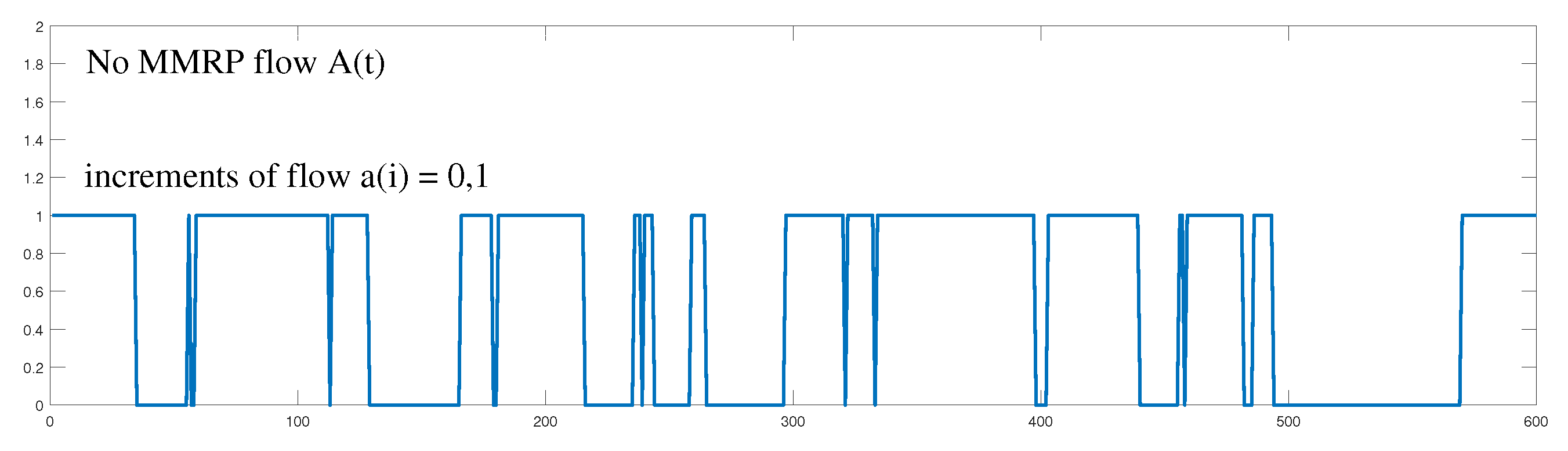
When modeling real IPTV traffic, we encountered flows that were clustered and contained alternating On and Off periods, but the probabilities of switching between periods could not be estimated because their values were outside the
interval. We present an example in
Figure 11.
We can see in the record that the flow in On periods has short outages. The need to model such flows led to the idea of turning on during the On period a Bernoulli process with a packet occurrence probability close to zero, .
6. Markov-Modulated Bernoulli Process
We have already dealt with the basic analysis of this process in the previous papers [
16,
17]. A Markov-modulated Bernoulli process is a process modulated by a two-state Markov chain, while a flow of units according to a Bernoulli process is transmitted during the On period with the parameter
p, or
; in the Off state, zeros are generated, which means that no traffic is broadcasted. A transition graph of the two-state Markov chain with discrete time is shown in
Figure 12:
The simulation of the MMBP process is significantly more complicated than the simulation of the Bernoulli process. If the source is in the On state, according to the probability
p, 1 or 0 is generated. Zero is generated even if the chain switches to the Off state. Switching between resource states is controlled using the transition probabilities
and
. Since the value 0 can be generated by two different elementary random events, we do not know, given the realization of the process, how to clearly describe the probabilities of events’ occurrence. In the following table, we show the realization of increments
with three different sequences of probabilities; see
Table 3:
Due to the ambiguity of the probability occurrence values of events 0 and 1, it is very problematic to derive the probability distribution of increments in the process and the probability distribution of gaps T.
We can model different types of flows by appropriate settings of parameters
,
, and
p. For
, we obtain all possibilities of the MMRP process. The Bernoulli process can be obtained in two ways: either
and
, or
. In the case that
, we obtain the flow that arises when tossing a fair coin. However, the most significant advantage of the MMBP usage is the acquisition of a flow which, in the On period, has short outages, or actually has two Off periods with different mean values of the silence period duration or non-broadcasting period. See
Figure 13.
6.1. Probability Distribution of MMBP
We calculate the probability distribution of flow increments in one elementary time slot using the complete probability theorem. First, we calculate the probability of generating a unit in an elementary time slot,
. The Markov chain
can only be in
(On) or
(Off) states at a given time. If it was in state
, (
),then it must remain in this state, (
), and generate 1 with probability
p. If it was in state
, (
), then it must go to state
, (
), and generate 1 again with probability
p:
The situation with
is significantly more complicated, because we have several possibilities for generating 0. If
was in state
, (
), it can remain in this state, (
), and generate 0 with probability
q or it can jump to state
,(
), in which it generates 0 for sure. If it was in state
, (
), it can remain in state (
) and generate 0, or it can go to state
, (
), and with probability
p generate 1:
After the adjustments, we found that in order for the stabilized chain to generate in time slot 1, it must be in state with success , and in order to generate 0, it must be in state and have failure, or be in state , in which it generates 0 automatically: . We will use this knowledge further in the derivation of the distribution .
We calculate the moments of the process
:
The mean and variance of the MMBP process coincide with the Bernoulli process . Flow modulation by a two-state chain has no effect on flow moments with increments of only .
We derive the probability distribution
using the knowledge obtained during the derivation of the distribution
:
We calculate the moments of the process
:
We expected that the mean value equals , as it is twice the mean occurrence of the value 1 in one elementary slot.
Dispersion is
If we put
, we obtain the dispersion of the MMRP process:
If
, the dispersion coincides with the Bernoulli process
:
It has a significantly more complicated form. Its value is influenced not only by the probabilities of switching between the
and
states, but also by the parameter
p.
In general, for the MMBP random process
, which represents the number of events in
n elementary slots, we can analytically express only the average rate, the probability of the peak occurrence, and of course the peak rate:
Thus far, we have only summarized and expanded the knowledge on MMRP and MMBP that we have already published in [
16,
17]. In the next chapter, we present newly derived knowledge about the probability distribution of the boundary
T in the MMBP process.
6.2. Probability Distribution of Time Spaces
In this chapter, we present our own way of deriving the hitherto-unknown probability distribution of time spaces for the MMBP model using a unique interconnection of various generation functions.
We will define the gap between packets in the MMBP process as a sequence of zeros (no packet occurred in the elementary slot), which will end the occurrence of the unit (packet). A gap can start by switching the source from the On state to the Off state, but by generating a 0 in the On state. A zero gap is represented by two consecutive units. For the probabilities
of the variable
T,
, the first values of
k, have the form:
The gap probability distribution is complicated, and we managed to derive the recurrence relation only for
:
In an effort to obtain probabilistic characteristics of the gap distribution, we decided to analyze the tail distribution function . The probability describes the occurrence of k consecutive zeros preceded by the occurrence of a unit.
The generation of 1 can only occur in the On state;
is the probability of occurrence of
k consecutive zeros if the process was in the On state. Therefore,
is equal to the probability of generating 0 in the On state or when switching to the Off state:
For the probability
, we have up to four possibilities to generate two consecutive zeros if the chain is in the On state at the beginning of generation:
The relation
is the probability of generating 0 if the chain is in the Off state. Let us call it
. We obtained the following recurrence relation for the probabilities
and
:
We receive a similar relationship for
. In total, we also have four possibilities to generate two consecutive zeros if the string is in the Off state:
So, let us denote by
the probability of generating consecutive
k zeros if the process is in the Off state. The probability
is equal to the product generation probabilities of 0 in the On state,
, and the probability of generating
zeros
, or the product of the probability of switching to the Off state,
, and generation probability
zero
. Similarly,
is equal to the product of the probability of generating 0 in the Off state,
, and the probability of generating
zeros
, or the product of the probability of switching to the On state and generating a zero,
, and the probability of generating
zeros
:
It holds that
. Let us define
. Then from Equations (
42) and (
43) hold for k = 1, 2, ….
To solve recurrence relations (
42) and (
43), we use generating functions
and
:
We derive the relation for the generating function
:
We derive the relation for the generating function
:
We obtain two relations between generating functions:
By solving the above equations, we get the form of the generating function
If we substitute
into the function
, we receive the generating function for the tail distribution of gaps in the MMRP process:
for the Tail distribution
:
Generating function
of the tail distribution
is decomposed into a Taylor series,
, while
has the form:
where
.
We obtain the probabilities
of the random variable
T from the differences of the tail distribution function:
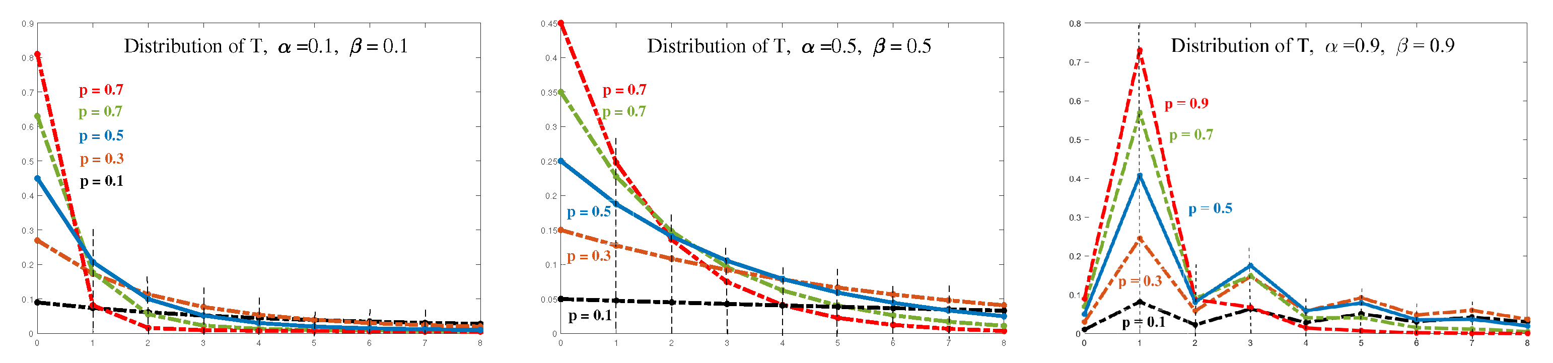
In general, the form of the probabilities
is complicated. However, it is not a problem to determine
for specific parameters. The following images show the probabilities of the distribution of
T with parameters
, and
. For the given parameters
and
, we gradually change the probabilities
p from
to
; see
Figure 14a–c:
Obtaining the explicit form of the probabilities from the function is problematic. Using the derivative, we can determine the first few values, but we were unable to develop the function into a power series.
6.3. Moments of Time Spaces
Using knowledge of the generation function form, we derive hitherto-unknown probabilistic characteristics of time space distribution: mean, variation, and third initial moment.
Using the function
, we can determine the moments of a random variable
T:
The random variable
has the same probability distribution as variable
T, but in the values
. It holds
and of course
. We obtain the form
by substituting
into the generating function
:
For the mean gap
, we receive some interesting formulas:
Variation of the stochastic variable
T is obtained from the derivative of the generating function
:
We obtained expressions for the second moments, initial and central moment, using the mean and derivative of the generating function at point 1.
We determine the value of the derivative
at a point
:
Using
, we obtain the second moments
and
:
We determine the coefficient of variability
from the derived moments of the random variable
T:
We derived the hitherto-unknown moments of the random variable describing the gaps in the MMBP On/Off process: mean
and variance
. Into the form
and
, we substitute
and
:
We obtain the already known mean
and variance
of the random variable
T describing the gaps in the MMRP process. Derivation of the third initial moment
is already considerably more complicated.
We break down the combination number and adjust it so that we receive the third power
:
We obtained expressions for the third initial moments using the mean value and the derivative of the generating function:
We do not specify the shape of
, we only determine it
:
If we substitute (
66) into (
65), we receive the analytical form of the third initial moment:
6.4. Estimation of MMBP Process Parameters
If we have a pcap file of measured traffic, we can estimate the values of the initial moments
,
, and
. From the mean
form, we obtain a recurrent relation between
and
:
By adjusting the relation (
59), we obtain the expression
using mean
:
If we know the estimates of the initial moments, then we can express
using
p:
If we substitute (
70) into the relation (
68), we get
The third initial moment has a complicated analytical form; therefore, we cannot use it to analytically estimate the parameter p, and we have to turn to numerical methods.
The parameter
p has values only in the interval
. Additional bounds are obtained from the condition
. From the condition
, we receive the lower bounds for
p:
If
would hold, then
. If we substitute the upper bound
into the relations (
70) and (
71), we receive the intervals for the parameters
a
:
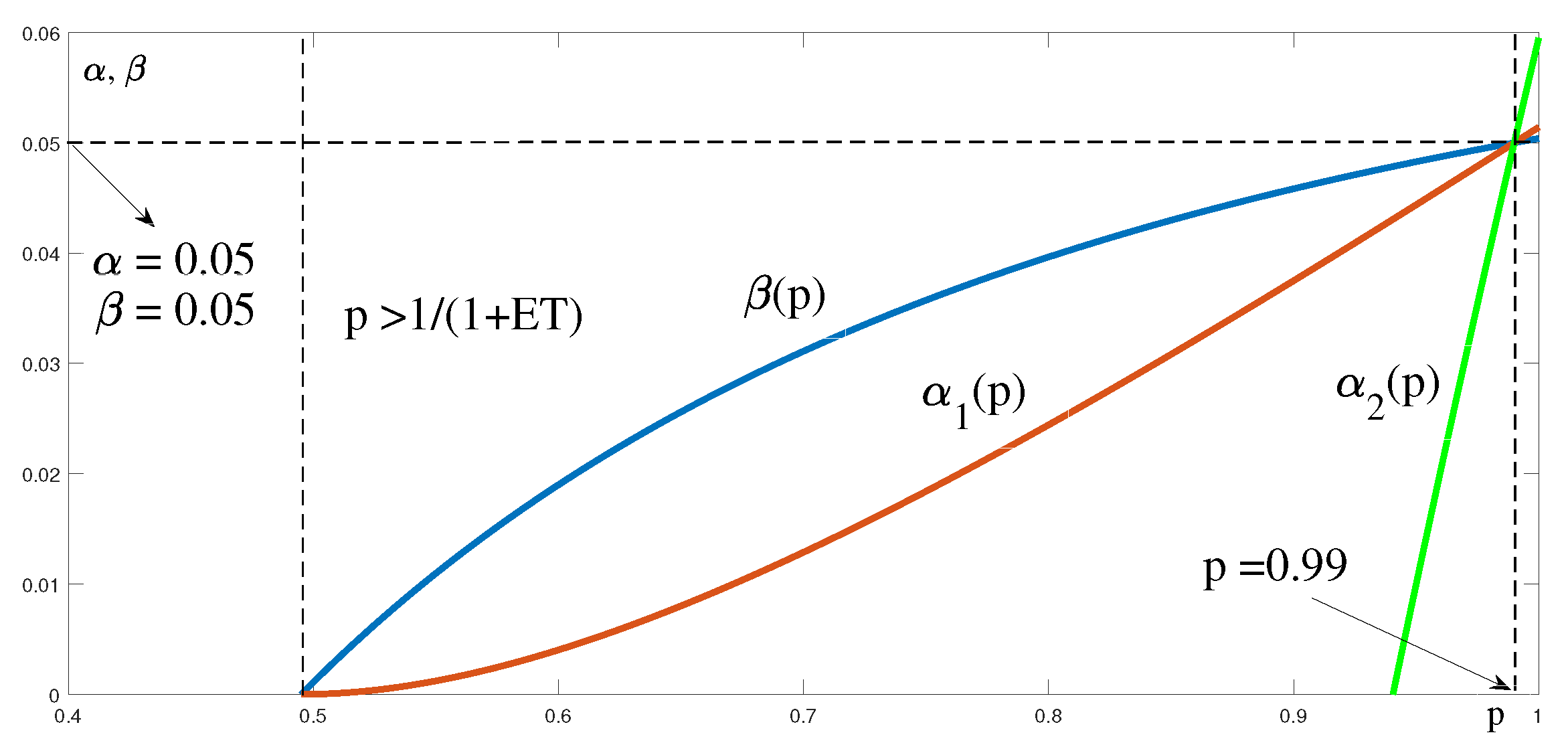
In the following figures, we can see the dependence of the parameters
and
on the probability
p, relations (
70) and (
71), for different estimates of
and
moments (
Figure 15):
For example, for the situation in which the moment estimates are and (the initial values of the parameters of the MMBP process are ), we get the lower bound of the probability . However, this range of values of the parameter p also satisfies both quadratic inequalities. In order to find the value of , we have to use numerical methods, for example, to find an upper estimate of the effective bandwidth of the measured traffic using the analytical form effective bandwidth of MMBP process (see the next chapter).
From the standard pcap file that contains captured IP traffic, after sampling for the selected time window of length
n, we can estimate the characteristics
,
, and
, for which we know it is true that
We use the formula for
and derive the necessary condition for the fast MMBP process recognition or rejection.
If the proportion of estimated values of mean and peak intensity differs statistically significantly from the estimated value , we can reject considerations of using the MMBP process for the given IP traffic.
For the missing estimate of the probability
p, we use the probability of the peak occurrence in the process
:
We obtained a second relation that expresses the dependence between
and
p and another lower bound for
p:
By numerically solving the equality between the relations (
71) and (
77), we can estimate the unknown parameter
p:
In relation (
79), we compared the estimate
obtained from the moments of the random variable
T and the estimate obtained from the average rate and probability of process peak
, which is created after sampling the original time record on
n time slots.
Let us go back to the IP traffic capture, which was the reason for exploring modeling using the MMBP process. In that capture, there was an alternation of On and Off periods, but the On periods had short interruptions; see
Figure 16a. By processing the time record, we obtained estimates of the moments:
ts,
ts
2. In order to calculate the average rate and probability of peak, we utilize sampling of the process to
n = 4 ts,
Figure 16b:
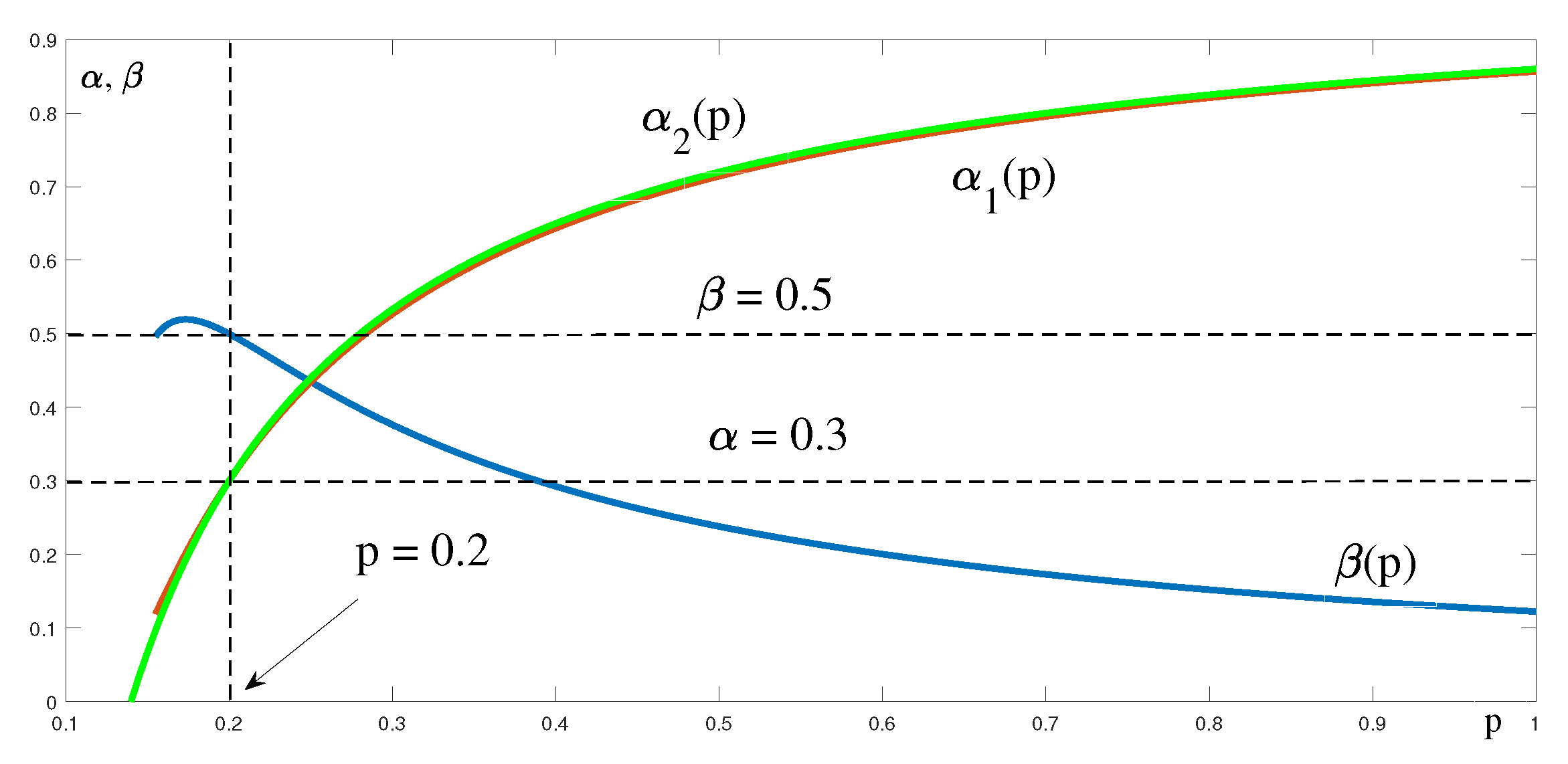
Functions in relations (
71) and (
77) will be denoted as
and
. From the equality of these two relations, we obtain the value of the parameter
p by numerical solution, and then, by substituting into the relations (
71) and (
70), we obtain the parameters
a
; see
Figure 17:
We expected the obtained parameter values. The 0/1 shape of the flow shows significant On and Off periods (calculated probabilities of staying in the states are 0.95), while short outages occur in the On period (probability of occurrence of 0 is 0.01).
Both probabilities of transitions between states are equal to , which means that the mean time of the Markov chain stay in both states is the same. We call such processes symmetric MMBP processes. In such a case, all three curves—, , and —must intersect at one common point.
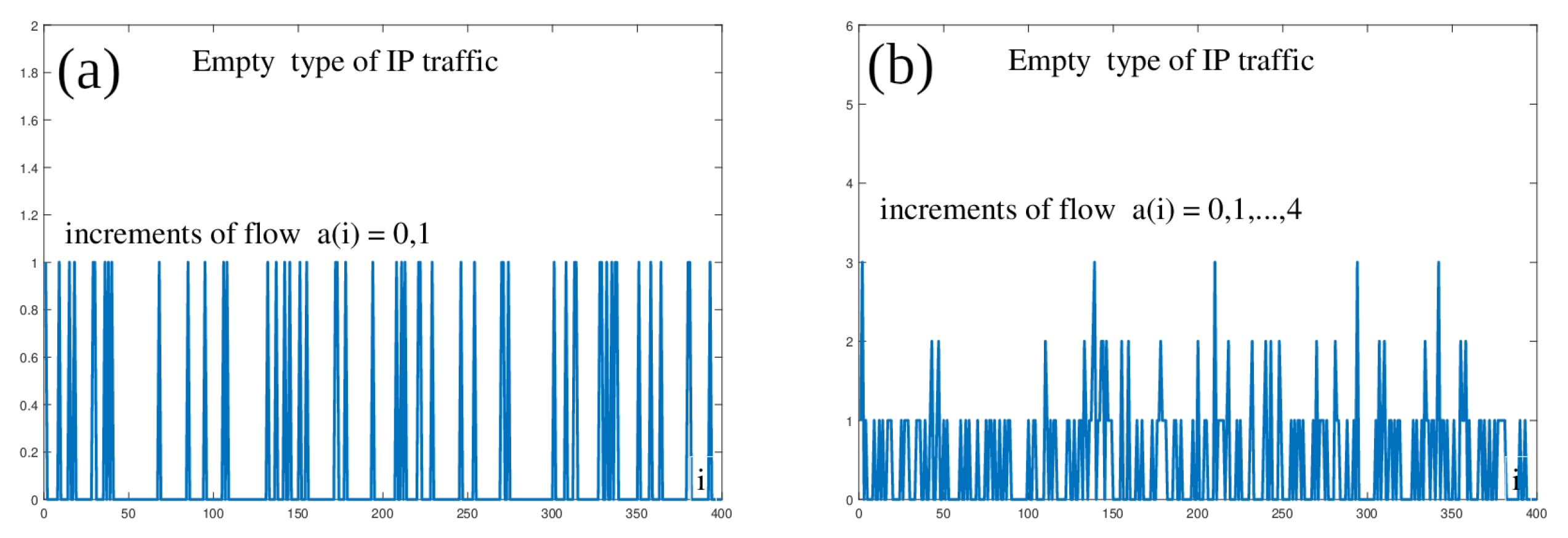
Thanks to its three parameters, the MMBP provides a wide range of different flow patterns. With the correct setting of the parameters, we can, for example, model the so-called empty flow with a rare occurrence of a packet in a time slot, as shown in
Figure 18a. By processing the time record and sampling to
, we obtained characteristics for
T and
; see
Figure 18b:
We obtained process parameters by numerical solution; see
Figure 19:
As the last example, we will show the type of process similar to the one we encountered during our experience with modeling IPTV operations for large ISP. In the 0/1 traffic capture, the process again shows significant On and Off periods, but during the On period, frequent alternation of 0 and 1 occurs in the time slot; see
Figure 20a. Characteristics for
T and
(see sampling,
Figure 20b):
We obtained process parameters; see solution
Figure 21:
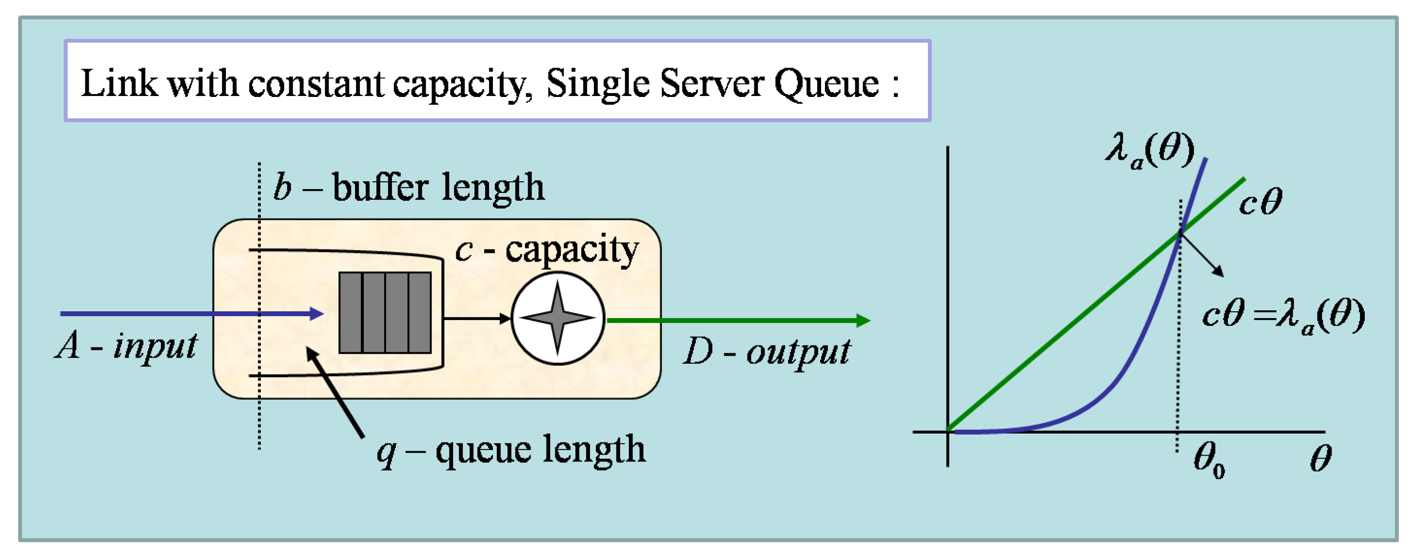
7. Use of Effective Bandwidth
The use of two-state Markov-modulated processes in IP flow modeling has the advantage that there is an analytical expression for these processes’ effective bandwidth. In such a case, we can relatively easily determine the necessary transmission speeds for given flows while guaranteeing the required QoS parameters: maximum delay d and probability of lost packet .
“The concept of effective bandwidth (EB) has gained much attention due to the looming gain for network analysis and design. The effective bandwidth of a general cumulative arrival process has been defined as” [
17]
“depending upon the space parameter
and the time parameter
t,
. The Theory of Large Deviation Principles provides the tool for link dimension with respect to probability of packet loss” [
17]
“where constant
b is the size of the queue (buffer) and variable
q is the steady-state length of the queue. If we propose a link capacity equal to the effective bandwidth,
, then the probability of buffer overflow decays (≍) exponentially with constant
” [
17].
“The value of effective bandwidth in 0 equals the average rate
. If the process has identical and above bounded increments,
, effective bandwidth is between the average rate and peak rate” [
17]:
“Let the process
have independent and identical distribution (i.i.d.) increments
. Let
be the moment generating function (MGF) and
be the cumulative generating function (CGF) of increments. EB has the form” [
17]:
Then, the tool for link dimensioning has the form (see
Figure 22):
For example, for the Bernoulli process (
), we gain the simple form of EB:
In general ([
18]), for any two-state Markov-modulated process, it holds that the moment generation function
of process is equal to the spectral radius
of matrix
, where
is a diagonal matrix of MGF functions
for the processes based on
states of Markov chain, and
is the matrix of the transition probabilities
Effective bandwidth for any MMP has the form
In order to determine the MGF , we must calculate the maximum eigenvalue of .
In the case of our On/Off MMBP, there are (
)
For the estimation of MGF
, we have to calculate the highest eigenvalue of matrix
. Then, CGF
has the form
The analytic solution for finding
and the EB of MMBP processes has the form
Figure 23 shows the EB for different symmetric MMBP with
and with the switch probabilities
. All models have the same
and
. For the same value of
, different EB values are obtained for different MMBP processes. The largest value,
, was obtained for the model with
. It is a process with distinct On and Off periods. In contrast, the process with
, which often switches between states and can be considered “almost” regular, acquired the smallest value,
. The value of
represents the minimum SSQ capacity necessary for fulfillment of the required QoS parameters, which is represented by the space parameter
. At the same average rate, the On/Off process is significantly more demanding on transmission network resources than the almost-regular process.
If the message is in the SSQ FIFO queue, then the maximum delay
d can be expressed using the queue size
b,
, where
c is the SSQ capacity. Tools for dimensioning () can be rewritten in the following form:
From the formula (
97), we can determine the relationship between the space parameter
and the QoS parameters (CGF is always a convex function; thus, the existence of an inverse function is guaranteed
):
If we have specified QoS parameters (
) for a given IP flow, we can use EB to set the capacity
c so that these QoS requirements are fulfilled:
For the MMBP process from the relations (
96) and (
99), we get an explicit formula for determining the required capacity
c with respect to the QoS parameters (
):
In case of On/Off MMRP, moment generation functions have the form
For the estimation of
, we have to calculate the highest eigenvalue of matrix
. Then, CGF
has the form
The analytic solution for finding
and the EB of MMBP processes has the form
Note that we would obtain the same values directly from the formula (
96) for the MMBP process by placing the probability value
.
After substituting the value
into the relation (
100), we obtain formulas for line capacity
c with the MMRP input process:
8. Problematic Modeling of IPTV Traffic
A limitation of the mentioned SSQ dimensioning method using effective bandwidth is the condition of finding the analytical form of the cumulative generating function and its inverse function. The MMBP process, since it depends on the three parameters , , and p, provides wide possibilities for different IP flows modeling, but it is not always sufficient. In such cases, however, this dimensioning method can still be used. A statistical estimate of the EB is calculated for the given flow, and the parameters , , and p are estimated using numerical methods so that the analytically corresponding shape of the EB is the upper limit of the statistical estimate. Finally, we will provide an example of such a situation.
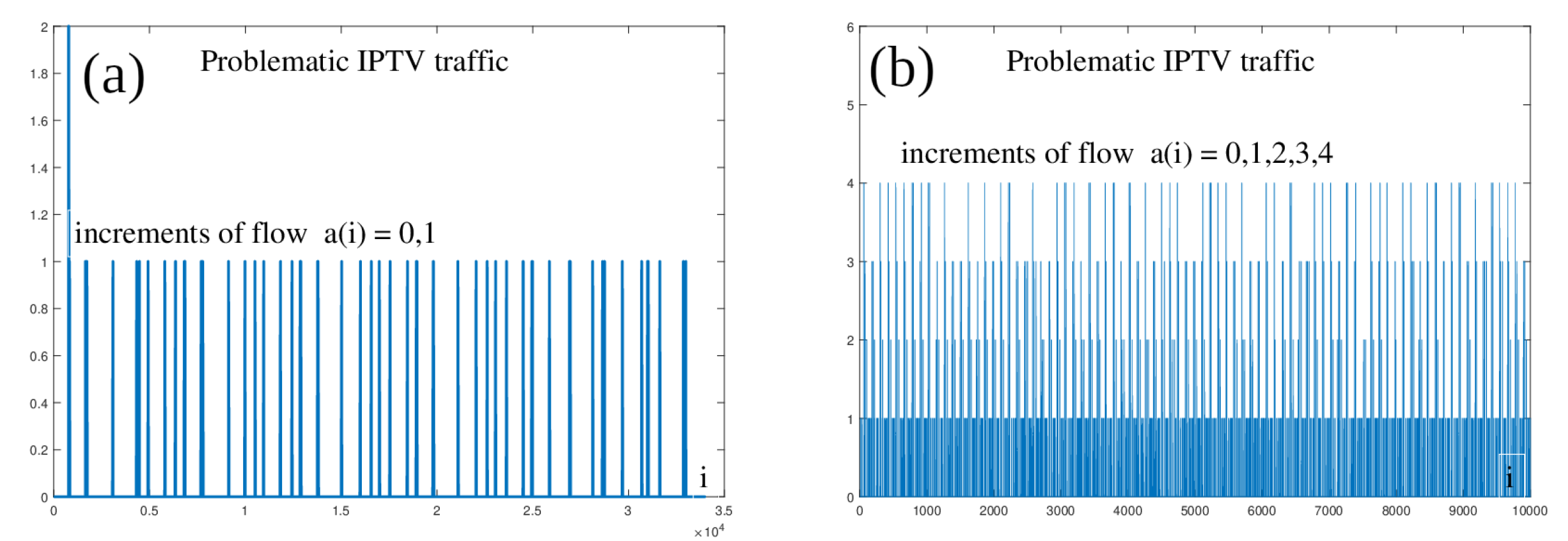
We are dealing with a sample of IPTV traffic, which was problematic to model using the MMBP process. It is a 2 min capture of one IPTV channel with a relatively static video (recording of a studio discussion); see
Figure 24a. In order to estimate the characteristics of
and
, we converted the sampling to
ms and thus, we obtained a record of the process
with increments
, as shown in
Figure 24b.
The characteristics of the variable
T and the sampled process
(
ms) are
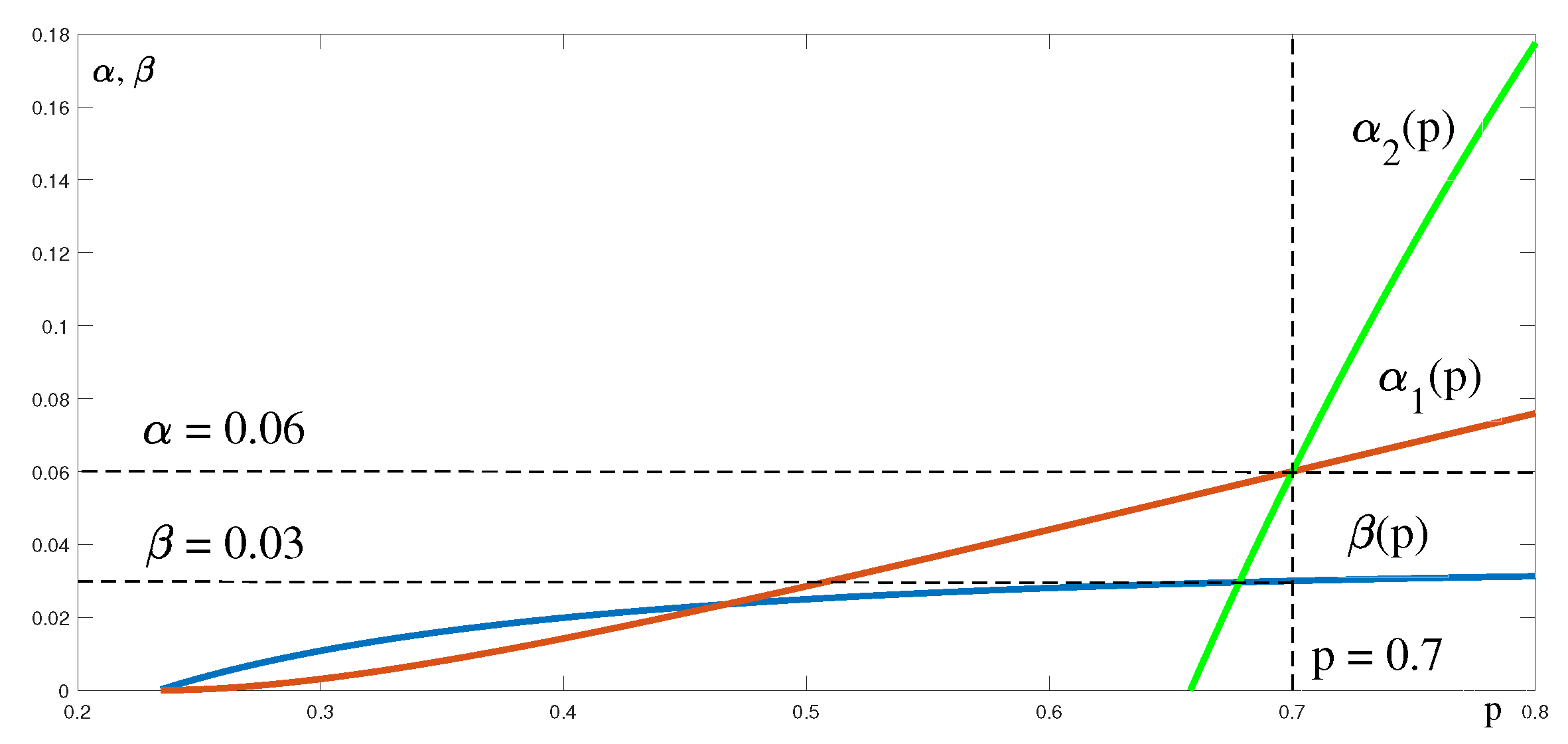
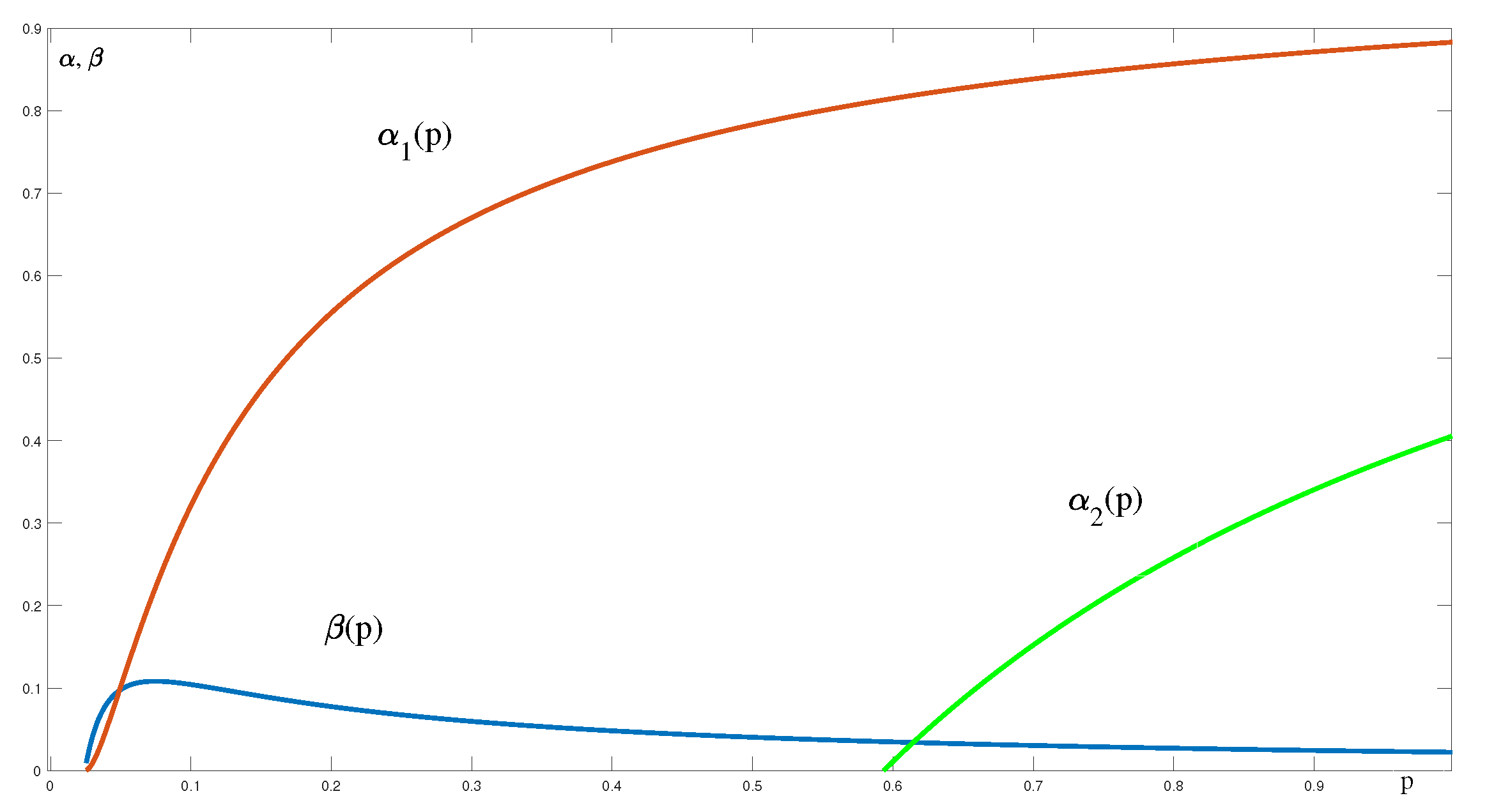
A problem occurred when estimating parameter
p using the curves
,
, and
. As we can see in
Figure 25, the curves
and
do not have a common intersection; therefore, the equation
does not have an interval
solution, meaning that the value of
p cannot be estimated; see
Figure 25.
We cannot model IPTV traffic using the MMBP process. However, we will show how to use the effective bandwidth of an MMBP process to estimate the line capacity for this IPTV stream with respect to QoS.
For any measured flow, we can always estimate the effective bandwidth. For a sampled process
, effective bandwidth has the form
For the analyzed IPTV stream, we estimated the parameters of the MMRP process using the relations (
25)
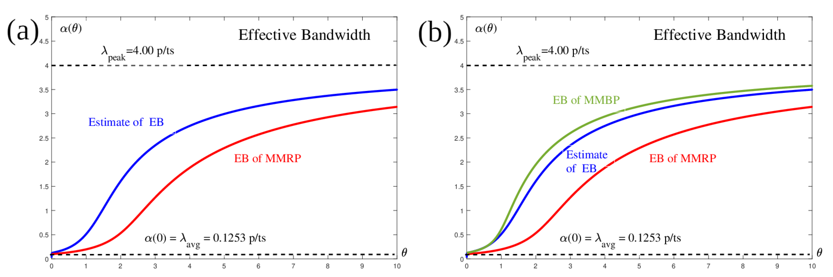
The reason why we try to find a suitable mathematical model for the analyzed traffic is the use of the analytical form of effective bandwidth to determine the necessary capacity of resources with respect to QoS. In
Figure 26a, we see that the use of the MMRP process as a model for IPTV operation is not suitable.
The effective bandwidth of MMRP at every point is significantly smaller than the statistical estimate of EB from measured traffic. Therefore, for some required QoS parameters (maximum delay and loss probability), we would obtain a smaller value of the required capacity than the value that would guarantee compliance with QoS for the given flow.
We used the estimated parameters of MMRP—
,
, and
—as starting values for calculating the parameters of the MMBP process, so that the EB of MMBP was the upper limit of statistical estimation of EB for IPTV flow. We obtained the values by numerical iterative methods.
,
and
; see
Figure 26b.
Parameter
is the so-called space parameter. If we consider the arrival process entering into some single server queue (a queuing system with one link), parameter
is directly dependent on a maximum delay
d of events waiting in queue, and on the probability of lost
. For the MMBP process, we calculate the
value using the following formula (
108):
For given QoS parameters of analyzed IPTV flow, for example
ms and
, according to (
108), the value of the space parameter is equal to
, and according to the relation (
96), the capacity needed to comply with QoS requirements is
p/ts; see
Figure 27.
We obtained a larger capacity value than we would receive from an exact IPTV stream model. From the dimensioning point of view with respect to QoS, we can state that we provide a higher guarantee of QoS fulfillment.
9. Conclusions
In the paper, we dealt with the use of two-state Markov-modulated processes for IP traffic modeling. We summarized and further developed the knowledge we have already published about the MMRP and MMBP processes, while for the sake of completeness, we also dealt with the basic Bernoulli process. In addition to basic analysis, we determined the necessary conditions for Bernoulli and MMRP processes for their use based on the estimation of the first and second initial moments of the random variable T, which describes the inter-arrival time between the occurrence of packets.
Next, we dealt with the method of estimating the parameters of the MMRP and MMBP process, which we called the peak equal method. Unlike the moment method, this method invokes, in addition to the equality of the average rate, the equality of the probabilities of peak occurrence in the flow.
The core of the article consists of our own derivation of the new probability distribution of MMBP process time spaces. First, we derived the generating function for the tail distribution of stochastic variable T. Expanding it to a power series, we obtained an explicit form of probabilities of tail distribution , which, however, had a complicated shape and were not suitable for further analytical use. For specific parameters of the MMBP process, we can use tail distribution to determine the probabilities of variable T, . Using the derivation of the generating function , we determined the first, second, and third initial moment of the variable T (and of course the variance), using the so-called combinatorial generating functions. Using a combination of the peak equal method and knowledge of the T variable moments, we created a new numerical method for determining the parameters of the MMBP process.
At the end, we presented the IPTV flow, which we were unable to model using the MMBP. However, thanks to the fact that the MMBP process has an analytical form of effective bandwidth, we managed to determine the capacity of the queuing system with respect to QoS for this flow as well.
Thanks to its flexibility (three parameters: , , and p), to the existence of effective bandwidth, and, last but not least, thanks to the derivation of the random variable T moments, the two-state MMBP On/Off process demonstrates significant potential for IP modeling operations for the purpose of dimensioning the IP network with regard to QoS parameters.


