Research on Financial Default Model with Stochastic Intensity Using Filtered Likelihood Method

Abstract

This paper investigates the financial default model with stochastic intensity by incomplete data. On the strength of the process-designated point process, the likelihood function of the model in the parameter estimation can be decomposed into the factor likelihood term and event likelihood term. The event likelihood term can be successfully estimated by the filtered likelihood method, and the factor likelihood term can be calculated in a standardized manner. The empirical study reveals that, under the filtered likelihood method, the first model outperforms the other in terms of parameter estimation efficiency, convergence speed, and estimation accuracy, and has a better prediction effect on the default data in China’s financial market, which can also be extended to other countries, which is of great significance in the default risk control of financial institutions.

1. Introduction

Generalized from stochastic processes, marked point processes have been widely applied in fields such as informatics, physics, and finance. A marked point process can be used to describe common bond defaults in financial markets [1], where the marker variable $U_n$ can be seen as the cumulative value of the default amount from zero to the corresponding moment [2]. Financial default models have been studied extensively by foreign academics. For example, Gordy et al. [3] developed the notion of rating-based bank capital risk and presented a single financial default model affected by visible systematic risk. Das et al. [4] and Duffie et al. [5] examined US financial default data from 1979 to 2004 and discovered that, in addition to observable systematic risk, all enterprises are vulnerable to unobservable systematic risk. Based on this, we present a model of the financial default with unobservable latent factors and an O-U process for studying the effect of latent variables on default intensity. Our study reveals that the model with latent variables is more accurate in depicting default events than the model with simply observable systematic risk. Azizpour et al. [6] also discovered that cluster contagion plays a crucial role in the dynamics of model parameters, and they put forward a financial default model that includes cluster contagion and latent variables. In this model, the latent variables are described by the conventional CIR model, and the cluster contagion is described by Hawkes’ standard self-excited process model [7]. The financial default model with the self-excited term outperforms the classic model when it comes to describing default events. Meanwhile, Chen et al. [8] applied the financial default model with the cluster contagion factor to give a derivation of the CDS pricing strategy based on this model, and proved that the financial default model with the cluster contagion factor also has better performance in the portrayal of default events in the supply chain system. Wang et al. [9] investigated how the non-financial sector affects the financial system, extended default clustering estimates to the non-financial sector using data on listed companies, and documented significant time-varying and cross-sectional changes in default clustering across different non-financial sectors in China. Finally, it was found that stock market volatility, fixed asset investment and credit-GDP gaps are key determinants of changes in time-series default clusters. Li et al. [10] proposed a simplified model for the embedded credit risk of corporate bonds. They specified the default risk rate as an affine function of a set of influencing variables and, in order to capture the clustering properties in certain extreme cases, employed a Hawkes jump-diffusion process to model these variables to derive a semi-analytical pricing formula for default bonds. Kai Xing et al. [11] found that macro indicators and NBER recession indicators are significant in explaining and predicting default clusters, even with a lag of 3 months.

The explanatory variables determining the default intensity in different financial default models are often different, and hence the estimation methods of the model parameters often differ from each other. On this premise, Ogata [12] proposed a point-process default model based on the experience of each state under complete data and proved the asymptotic property and convergence of its parameter estimation method on this basis. Fernando et al. [13] investigated the situation in which the model’s default intensity is based on the proportional risk equation with complete data. However, in the default model generated from incomplete observable data (partially observable or unobservable explanatory variables), the discrete information flow of partially observable variables and the path dependence of endogenous variables cause the filtering problem of discontinuous information flow due to the interaction of explanatory variables and point-process paths in the intensity parameters. Most researchers utilize interpolation to make the trajectories of some observable variables continuous in the filtering problem. For example, Lando [14] extended the COX model to give parameter estimates for a financial default model based on default intensity with latent variables under incomplete observable data. In previous studies, it was found that using the interpolation method to solve the likelihood function does not lead to a closed-form solution, and the properties of the resulting parameter estimation method are not well described. Thus, it is reasonable to attempt methods other than interpolation to solve the filtering equations controlling the maximum likelihood estimation. Elliott et al. [15] used a stochastic EM technique to solve the filtering equations and provide asymptotic estimates of the filtering control equations. Giesecke et al. [16] suggested a method for estimating the default intensity based on filtered likelihood estimation and obtained an analytical solution for parameter estimation. The filtered likelihood technique outperforms other methods for solving the filtered equations in terms of parameter estimation accuracy and asymptotic efficiency in numerical simulations. This method can be seen as a good answer to the default model’s parameter estimation problem with incomplete observable data.

Clusters of corporate defaults can have catastrophic economic effects, such as a sudden drop in consumption [17]. The default behavior is one of the most important indicators for credit rating review in the financial market. However, financial default modeling and estimation methods in China are still in their infancy, relying primarily on basic models and Monte Carlo simulation approaches. The filtered likelihood estimation approach is rarely employed in China since there is a lack of the effective creation of explanatory variables affecting financial default events. Studying financial default, particularly bond default, is critical both theoretically and practically for avoiding financial risk and establishing a stable financial environment. Based on incomplete observable data, a filtered likelihood estimation method is utilized in this research to estimate the parameters of the marked point process under the influence of self-excitation and jump-diffusion processes on the default intensity [18]. We also compare and analyze the parameter estimation and model-fitting effects of the two models, as well as investigating and analyzing China’s financial default problem and development trend, using financial default data from 2014 to 2020 [19], and find that our first model has better results in portraying the small sample data of the Chinese bond default market. Other references are also of great help to this paper [20,21,22,23,24].

2. Explanation of Related Concepts

2.1. The CIR Process

The O-U process is a stochastic process, also known as the Ornstein–Uhlenbeck process, which describes a stochastic process with a tendency to regress to the mean. Originally invented by Ornstein and Uhlenbeck in the 1930s, the O-U process is widely used in finance, physics, chemistry, biology, and other fields. The O-U process is usually described by the following differential equation:

$$dX\left(t\right)=\theta (\mu -X(t\left)\right)dt+\sigma dW\left(t\right)$$

where $X\left(t\right)$ is the value of the stochastic process at time t, and $\theta ,\mu ,\sigma$, and $W\left(t\right)$ represent the regression intensity, mean, standard deviation, and Wiener process, respectively. The Wiener process is a continuous, constantly changing stochastic process, which is the noise source of the O-U process and represents the stochastic fluctuations in the system.

In the O-U process, the random variable $X\left(t\right)$ fluctuates up and down around the mean value $\mu$, but when $X\left(t\right)$ deviates from the mean, the regression force $\theta$ tends to pull it back to the mean. Thus, the O-U process has the property of regression to the mean, which makes it useful in describing random walks (i.e., random wanderings).

The O-U process and the CIR process are solutions of stochastic differential equations, and they both have the property of regression to the mean, which can be used to describe the evolution of stochastic processes, and therefore they both have a wide range of applications in the field of finance. In fact, the CIR process can be regarded as an extension of the O-U process, and there are certain connections and similarities between them. Specifically, the CIR process can be obtained by applying some transformations to the O-U process. Suppose we have a random variable $X\left(t\right)$ that conforms to the O-U process, which can be expressed as

$$dX\left(t\right)=\theta (\mu -X(t\left)\right)dt+\sigma dW\left(t\right)$$

where $\theta$ is the regression intensity, $\mu$ is the mean, $\sigma$ is the standard deviation, and $W\left(t\right)$ is the Wiener process. We can transform it as follows:

$$\begin{array}{cc}\hfill r\left(t\right)& =X{\left(t\right)}^2\hfill \\ \hfill dr\left(t\right)& =2X\left(t\right)dX\left(t\right)+{\left(dX\left(t\right)\right)}^2\hfill \end{array}$$

Substituting the differential equation for $X\left(t\right)$ into the above equation, we obtain

$$dr\left(t\right)=2X\left(t\right)(\theta (\mu -X\left(t\right))dt+\sigma dW\left(t\right))+{\sigma }^2{\left(dW\left(t\right)\right)}^2$$

The simplification gives

$$dr\left(t\right)=2\theta (\mu -X\left(t\right))X\left(t\right)dt+{\sigma }^{2}dW\left(t\right)$$

This equation is very similar to the form of the equation for the CIR process, and by simply considering $r\left(t\right)$ as the random variable of the CIR process, $\kappa =2\theta$, $\theta =2\theta \mu /{\sigma }^2$, and $\sigma =\sigma$, we can obtain the form of the equation for the CIR process as follows

$$dr\left(t\right)=\kappa (\theta -r\left(t\right))dt+\sigma \sqrt{r\left(t\right)}dW\left(t\right)$$

Therefore, the CIR process can be regarded as an extension of the O-U process, an extended model based on the O-U process, which is widely used in finance for interest rate modeling, option pricing, etc.

2.2. The Cox Process

The Cox model is a statistical model for analyzing survival data, which was originally proposed by David Cox in 1972 and is widely used in survival analysis in medicine, public health, finance, etc. The Cox model is a semi-parametric model that can handle right-hand truncated survival data and does not require any assumptions about the time distribution. The ratio comparison analyzes the effect of a factor on survival time by comparing the risk ratio of two groups on that factor. The basic form of the Cox model is as follows:

$$h\left(t\right|X)=h_0\left(t\right)exp({\beta }_1{X}_1+{\beta }_2{X}_2+\cdots +{\beta }_p{X}_p)$$

where $h\left(t\right|X)$ represents the risk function at time t given the covariates X, $h_0\left(t\right)$ is the underlying risk function, and ${\beta }_1,{\beta }_2,\cdots ,{\beta }_p$ are the coefficients of the covariates $X_1,X_2,\cdots ,X_p$. The core of the Cox model is the assumption that the risk function can be decomposed into an exponential function of the underlying risk function and covariates, which allows the Cox model to handle a variety of different risk factors and does not require any assumptions to be made about the underlying risk function.

2.3. The Hawkes Process

The Hawkes process (Hawkes process) is a stochastic process, which was proposed by Hawkes in 1971 to describe the stochastic process of a class of events occurring. The Hawkes process is often used to describe the occurrence and evolution of events, such as social networks, financial markets, and earthquakes. The Hawkes process has the property of self-excitation, that is, the occurrence of one event affects the occurrence probability of subsequent events.

The basic form of the Hawkes process is as follows:

$$\lambda \left(t\right)=\mu \left(t\right)+\sum _{i=1}^{N\left(t\right)}g(t-t_i)$$

where $\lambda \left(t\right)$ represents the intensity function at time t, $\mu \left(t\right)$ is the underlying intensity function, $N\left(t\right)$ is the event count in the time interval $[0,t]$, and $g(t-t_i)$ is the activation function that affects the probability of subsequent events. The central idea of the Hawkes process is that when an event occurs, it has an effect on the probability of occurrence of subsequent events, and this effect can be described by the activation function $g(t-t_i)$. The activation function $g(t-t_i)$ represents the effect of an event occurring at time $t_i$ on an event after time t, and it is usually a non-negative function with respect to the time difference $t-t_i$.

The model parameters of the Hawkes process can be estimated by the maximum likelihood estimation, which can be implemented using the Hawkes package in the R language. The model parameters of the Hawkes process include the underlying intensity function $\mu \left(t\right)$ and the activation function $g(t-t_i)$, etc. By studying these parameters, the pattern of event occurrence can be obtained, and the occurrence of future events can be predicted.

In conclusion, the Hawkes process is a stochastic process used to describe the occurrence of events, which has the property of self-excitation and can be used to describe the occurrence and evolution of events such as social networks, financial markets, and earthquakes. The estimation and prediction of the Hawkes process model parameters can be achieved by the maximum likelihood estimation and analysis of the activation function.

3. Financial Default Marked Point Process Model

A complete probability space $(\mathsf{\Omega },F,P)$ and a right continuous and complete filtration ${\left({\mathcal{F}}_t\right)}_{t\ge 0}$ are fixed, and a marked point process $\left(T_n,U_n\right)$ is conducted. The $T_n$ is a strictly increasing sequence of positive stopping times that represent the arrival times of events. The $U_n$ is ${\mathcal{F}}_{T_{n-}}$ measurable mark variables that take values in a subset $R_U$ of the Euclidean space. The marked point processes $\left(T_n,U_n\right)$ provide information about the arrival of events. One of the random processes $N_t$ is also called the counting process used to calculate the number of event arrivals:

$$N_t={\sum }_{n\ge 1}^{}{I}_{(T_n\le t)}$$

(1)

Because $N_t$ contains the same information as the stop-time sequence, it can act as a replacement for the stop-time sequence. $N_t$ has a right continuous time-dependent violation strength ${\lambda }_t$:

$${\lambda }_t=\mathsf{\Lambda }(V;\alpha )$$

(2)

where $\mathsf{\Lambda }$ is a function determined by the parameter $\alpha$, $V_t$ denotes a Markov process taking values in $R_V$. The initial value of this process and the transfer probability are determined by the parameter $\gamma$. The conditional distribution function ${\pi }_t$ of the marker variable $U_n$ is determined by the parameter $\beta$:

$$\begin{array}{c}\mathsf{\Lambda }:R_v\to (0,\infty )\hfill \\ {\pi }_t\left(d_u\right)=\pi (u,V_t;\beta )d_u\hfill \end{array}$$

(3)

After the initial values and the corresponding state transfer probabilities are given, the intensity of the default event arrival ${\lambda }_t$ and the process of the explanatory variable $V_t$ are dynamically changed. Here, $V_t$ and $N_t$ are interacting. In particular, $N_t$ can appear as a constituent element in $V_t$, or $V_t$ and $N_t$ have the same jump or self-excited behavior. Specifically, the structure of the explanatory variable stochastic process $V_t$ can be set as $\left(X,Y,Z\right)$, where X represents the observable explanatory variable and the path of X in $\left(0,t\right)$ can take values in $R_X$, Y represents the partially observable explanatory variable and the path of Y in $\left(0,t\right)$ takes values in $R_Y$, and Z represents the unobservable latent variable and the path of Z in $\left(0,t\right)$ takes values in $R_Z$, which is shown in Equation (4). Order $\tau$ is the time of the first default:

$$\begin{array}{c}{N}_{\tau }=\left\{N_t:0\le t\le \tau \right\}\hfill \\ U_{\tau }=\left\{{\sum }_{n\le N_t}{U}_n:0\le t\le \tau \right\}\hfill \\ X_{\tau }=\left\{X_t:0\le t\le \tau \right\}\hfill \\ Y_{\tau }=\left\{Y_t^j:0\le t\le \tau ,t\in s^j\right\},j\in \left\{1\cdots d_y\right\},s=\bigcap _{j=1}^{d_y}{s}_j\ne \varnothing ,d_y>0,d_z>0\hfill \end{array}$$

(4)

Since the default intensity of financial default events arrival is influenced by macro- and micro-economic factors, observable systematic risk variables, and unobservable systematic risk variables, the structure of the default intensity is constructed as shown in Equation (4) in the setting of the default intensity:

$${\lambda }_t=\sum _{i=1}^d{a}_i{X}_{i,t}+Y_t+Z_t$$

(5)

4. Filter Likelihood Method

The filtered likelihood asymptotic method was proposed by Giesecke et al. [16]. On the one hand, it solves the problems of difficulty in describing the nature of the solution results and difficulty in controlling the convergence speed when the traditional interpolation method is used for parameter estimation of the violation intensity of the marked point process. On the other hand, it also solves the problems of path dependence and discontinuous information flow when the partially observable variable $Y_t$ is calculated under incomplete data. The filtered likelihood method is superior in terms of parameter accuracy, parameter convergence speed and asymptotic efficiency. Therefore, the filtered likelihood method is used as the parameter estimation method for the financial default intensity model.

First let the parameters be estimated for the explanatory variables in the point process with default intensity as $\theta =(\alpha ,\beta ,\gamma )\in \mathsf{\Theta }$. The true unknown parameters ${\theta }^0\in {\mathsf{\Theta }}^0$, $P_{\theta }$ and $E_{\theta }$ denote the probability and expectation operators, respectively. Then, the likelihood function $L_{\tau }\left(\theta \right)$ of the data $D_{\tau }$ under the parameter $\theta$ comes from the Radon–Nikodym derivative of the $P_{\theta }$ distribution. Under incomplete data, the likelihood function is a projection of $\frac{d{P}_{\theta }}{d{P}_{{\theta }_0}}$, so we have

$$L_{\tau }\left(\theta \right)=E_{{\theta }_0}\left[\frac{d{P}_{\theta }}{d{P}_{{\theta }_0}}|D_{\tau }\right].$$

(6)

Set the random variable $M_{\tau }\left(\theta \right)$ and the distribution function ${\pi }^{*}\left(U_n\right)$ of the marker term. When $E_{\theta }\left[M_t\left(\theta \right)\right]=1$ in Equation (7) satisfies the condition, a new measure $P_{\theta }^{*}$ can be obtained. The counting process in the point process under the new measure obeys the standard Poisson distribution, and the distribution function of the marker term is also independent of $\theta$ [16]:

$$M_{\tau }\left(\theta \right)=\prod _{n\le N_{\tau }}\frac{{\pi }^{*}\left(U_n\right)}{\pi \left(U_n,V_{T_n-;};\beta \right)}\ast exp\left(-{\int }_0^{\tau }log\left(\mathsf{\Lambda }\left(V_{s-};\alpha \right)\right)d{N}_s-{\int }_0^{\tau }\left(1-\mathsf{\Lambda }\left(V_s;\alpha \right)\right)ds\right).$$

(7)

Therefore, when the parameters are estimated under incomplete data, $L_{\tau }\left(\theta \right)$ can be calculated by splitting it into the product of the point process term and the explanatory variable term. See Theorem 1 and Equation (8):

$$L_{\tau }\left(\theta \right)=log{L}_F^{*}\left(\theta ;\tau \right)+log{L}_E^{*}\left(\theta ;\tau \right).$$

(8)

In the calculation of Equation (8), a more standardized solution for the term $log{L}_F^{*}\left(\theta ;\tau \right)$ is already available [8,14]. However, it is more difficult to calculate the direct solution for $log{L}_E^{*}\left(\theta ;\tau \right)$. Thus, the likelihood asymptotic is performed using the filtered likelihood method for the term $\epsilon \left(\theta ;\tau ,g\right)$ in the following Equation (9):

$$\epsilon \left(\theta ;\tau ,g\right)=E_{{\theta }^{*}}\left[\frac{g\left(V_{\tau },\tau \right)}{M_{t\left(\theta \right)}}|D_{\tau }\right].$$

(9)

According to Theorem 1, when $g\left(V_{\tau },\tau \right)=1$, $log{L}_E^{*}\left(\theta ;\tau \right)$ can be calculated. Therefore, we divide the state space by $m_s\in \mathbb{N}$ and the time interval by $m_T\in \mathbb{N}$ to obtain $E^I(\theta ;\tau ,g)$ as its likelihood approximation. The specific result is shown in (10):

$$E^I(\theta ;\tau ,g)=\sum _{i_0=1}^{m_s}\dots \sum _{i_{m_t}=1}^{m_s}{p}_{\theta ,0}^I\left(i_0\right)\times \prod _{j=1}^{m_T}{W}_{\theta ,j}^I\left(i_j\right)p_{\theta ,j}^I\left(i_j,i_{j-1}\right).$$

(10)

$p_{\theta ,0}^I\left(i_0\right)$ and $W_{\theta ,j}^I\left(i_j\right)$ in Equation (10) are given in a more complicated form ([14]) and are not given here. $E^I\left(\theta ;\tau ,1\right)$ can be viewed as an approximation of $\epsilon (\theta ;\tau ,1)$ based on the multidimensional rectangular orthogonal Leberg integral. In the calculation of $E^I\left(\theta ;\tau ,1\right)$, if the $m_s^{m_T}$ orbits (realizations) are multiplied, finding the parameter estimate that maximizes the probability of all states occurring is difficult to achieve. Therefore, the filtered likelihood algorithm is used to adjust the construction order of the likelihood function, and the transfer probability matrix is constructed from the transfer probabilities p of all states at each moment t. The $log{L}_E^{*}\left(\theta ;\tau \right)$ term is solved by the dot product of the matrix and the multiplication of the matrix, and the local optimal solution of the log-likelihood function is finally solved by the simplex method.

First the vector $\xi$ is constructed, where $\xi \left(i\right)$ is the component of $\xi$, $1\le i\le m_s$. Next, since the asymptotic essence of $E^I(\theta ;\tau ,1)$ is the integral of all realization paths based on a sufficiently small time interval and the division of the state space. For each initial state of $p_{\theta ,0}^I\left(i_0\right)$ with a probability of that, the integral of the realization path term that should be obtained is shown in (11):

$$\sum _{k=1}^{m_s}{p}_{\theta ,0}^I\left(i\right)\times p_{\theta ,j}^I(k,i).$$

(11)

Therefore, the matrix calculation is used, and the specific calculation process is divided into two steps.

First, the explanatory variables transfer probability matrix is constructed as shown in (12). The integral of the realized path is calculated up to moment $m_T$. Then $\xi$ is updated:

$$\begin{array}{l}{Q}_j=\left[\begin{array}{ccc}{q}_j(1,1)& \dots & q_j\left(1,m_s\right)\\ ⋮& ⋮& ⋮\\ q_j\left(m_s,1\right)& \dots & q_j\left(m_s,m_s\right)\end{array}\right]\\ q_j(k,l)=W_{\theta ,j}^I\left(k\right)\times P_{\theta ,j}^I(k,l)\\ k,l\in 1\dots m_s\\ j\in 1,\dots ,m_T-1\\ \xi \leftarrow Q_j\ast \xi \end{array}$$

(12)

Next, the operation in Equation (13) is performed to construct the probability function matrix at moment $m_T$ and accordingly calculate the integral of the realized path at moment $m_T$ and update it for $\xi$:

$$\begin{array}{c}{Q}_{m_T}=\left[\begin{array}{ccc}{q}_{m_T}(1,1)& \dots & q_{m_T}\left(1,m_s\right)\\ ⋮& ⋮& ⋮\\ q_{m_T}\left(m_s,1\right)& \dots & q_{m_T}\left(m_s,m_s\right)\end{array}\right]\hfill \\ q_j(k,l)=W_{\theta ,m_T}^I\left(k\right)\times P_{\theta ,m_T}^I(k,l)\hfill \\ k,l\in 1\dots m_s\hfill \\ \xi \leftarrow Q_{m_T}\ast \xi \hfill \end{array}$$

(13)

The final summation of the realized path integrals for all initial states yields an approximation $E^I\left(\theta ,\tau ,1\right)$ for $\epsilon \left(\theta ;\tau ,1\right)$, which is shown in Equation (14).

$$E^I(\theta ;\tau ,1)=\sum _{i=1}^{m_s}\xi \left(i\right)$$

(14)

After the algorithm is constructed, the state space and the time interval are divided into $m_s$ and $m_T$ intervals. Then, the unobservable explanatory variables $Z_t$ and the partially observable explanatory variables $Y_t$ are transformed into matrices (the expressions are available in the subsequent sections). The orbits (realizations) of the point process are combined and logarithmically manipulated, which are also combined with the log-likelihood function $log{L}_F^{*}\left(\theta ;\tau \right)$ for the explanatory variables part of the processed incomplete data to derive the filtered likelihood asymptotic $\epsilon \left(\theta ;\tau ,g\right)$ for the point process events and the stopping time part. The local optimal solution of the log-likelihood function is found via the downhill simplex method. The parameter estimates obtained by the filter likelihood method can be obtained.

5. Properties and Proofs of Filtered Likelihood Estimation

Since it is known that it is difficult to solve $L_{\tau }\left(\theta \right)$ directly after the Radon–Nikodym transformation, the random variable $M_{\tau }\left(\theta \right)$ and the distribution function ${\pi }^{*}\left(U_n\right)$ of the marker term are set. The likelihood function can be calculated in two parts when the condition $E_{\theta }\left[M_{\tau }\left(\theta \right)\right]=1$ is satisfied. The sum of the two independently calculated parts, i.e., the event term $log{L}_E^{*}\left(\theta ;\tau \right)$ and the factor term $log{L}_F^{*}\left(\theta ;\tau \right)$, which is positively correlated with the initial maximum likelihood function $L_{\tau }\left(\theta \right)$, i.e., the direction of the optimal solution parameters, is the same. The following theorem applies:

Theorem 1. 

Assume that the following conditions hold:

(1) On parameter space Θ, $E_{\theta }\left[M_{\tau }\left(\theta \right)\right]=1$ is satisfied for all $\theta \in \mathsf{\Theta }$;

(2) For all $\theta \in \mathsf{\Theta }$, given the event data $\left(N_{\tau },U_{\tau }\right)$ under measure $P_{\theta }^{*}$, the conditional likelihood function $log{L}_f^{*}\left(\theta ;\tau \right)$ for the factor data $(X_{\tau },Y_{\tau })$ exists and is strictly positive a.s., then the likelihood function is satisfied:

$$\begin{array}{c}{L}_{\tau }\left(\theta \right)\propto E_{\theta }^{*}\left[\frac{1}{M_{\tau }\left(\theta \right)}\mid D_{\tau }\right]·log{L}_F^{*}(\theta ;\tau ).\hfill \end{array}$$

(15)

The above theorem gives a method for estimating the posterior probability and the posterior mean of the filtered likelihood based on incomplete data. The results of the parameter estimation of the filtered likelihood have the same optimization direction as the original maximum likelihood function, which is proved as follows.

Proof of Theorem 1. 

From condition (1) and the definition of the measure $P_{\theta }^{*}$, we have $d{P}_{\theta }^{*}=M_{\tau }\left(\theta \right)d{P}_{\theta }$, so for any $A\in D_{\tau }$, the measure $P_{\theta }^{*}$ and the measure $P_{\theta }$ can be transformed as in (16):

$$\begin{array}{c}{P}_{\theta ,\tau }\left(A\right)=E_{\theta }\left[1_A\right]=E_{\theta }^{*}\left[1_A{E}_{\theta }^{*}\left[\frac{1}{M_{\tau }\left(\theta \right)}\mid D_{\tau }\right]\right]={\int }_A{E}_{\theta }^{*}\left[\frac{1}{M_{\tau }\left(\theta \right)}\mid D_{\tau }\right]d{P}_{\theta ,\tau }^{*}.\hfill \end{array}$$

(16)

According to the Radon–Nikodym theorem, the measure $P_{\theta }^{*}$ is absolutely continuous with respect to measure $P_{\theta }$ under the Radon–Nikodym derivative, so Equation (17) is established:

$$\begin{array}{c}\frac{d{P}_{\theta ,\tau }}{d{P}_{\theta ,\tau }^{*}}=E_{\theta }^{*}\left[\frac{1}{M_{\tau }\left(\theta \right)}\mid D_{\tau }\right]\hfill \end{array}$$

(17)

Then, according to the Bayesian formula, the measure of the data under $P_{\theta }^{*}$ is equal to the product of the measure of the event term $\left(N_{\tau },U_{\tau }\right)$ under $P_{\theta }^{*}$ and the posterior conditional probability of the factor data $\left(X_{\tau },Y_{\tau }\right)$ under the given event term

$$\begin{array}{ccc}\hfill P_{\theta ,\tau }^{*}& =& P_{F,\theta ,\tau }^{*}{P}_{E,\theta ,\tau }^{*}.\hfill \end{array}$$

(18)

Since the event term $\left(N_{\tau },U_{\tau }\right)$ does not depend on the parameter $\theta$ under the measure $P_{\theta }^{*}$, the counting process N is normalized. Also, the density function ${\pi }^{*}$ of the labeled term under the measure $P_{\theta }^{*}$ does not depend on parameters $\theta$ and ${\theta }_0$, so Equation (19) holds:

$$\begin{array}{c}\hfill \frac{P_{E,\theta ,\tau }^{*}}{P_{E,{\theta }_0,\tau }^{*}}\propto 1.\end{array}$$

(19)

Equation (20) can be obtained by condition (2):

$$\begin{array}{c}\hfill \frac{P_{F,\theta ,\tau }^{*}}{P_{F,{\theta }_0,\tau }^{*}}=L_F^{*}(\theta ;\tau ).\end{array}$$

(20)

Since $P_{\theta }^{*}$ is in the form of a product of measures as shown in Equation (18), it is obtained by combining Equation (19) with (20) and using Fubini’s theorem:

$$\begin{array}{c}\hfill \frac{d{P}_{\theta ,\tau }^{*}}{d{P}_{{\theta }_0,\tau }^{*}}=\frac{d{P}_{F,\theta ,\tau }^{*}·d{P}_{E,\theta ,\tau }^{*}}{d{P}_{F,{\theta }_0,\tau }^{*}·d{P}_{E,{\theta }_0,\tau }^{*}}=\frac{d{P}_{F,\theta ,\tau }^{*}}{d{P}_{F,{\theta }_0,\tau }^{*}}·\frac{d{P}_{E,\theta ,\tau }^{*}}{d{P}_{E,{\theta }_0,\tau }^{*}}\propto L_F^{*}(\theta ;\tau ).\end{array}$$

(21)

In summary, the filtered likelihood function has the same optimization direction as the original likelihood function, i.e.,

$$\begin{array}{c}\hfill L_{\tau }\left(\theta \right)\propto E_{\theta }^{*}\left[\frac{1}{M_{\tau }\left(\theta \right)}\mid D_{\tau }\right]·log{L}_F^{*}(\theta ;\tau ).\end{array}$$

(22)

□

6. Two Intensity Parameter Models

The default intensity can usually be expressed in the form of Equation (23), where p represents the arrival rate of a default event in time h. We multiply it by the number of defaults, divide it by the time interval h, and take the limit, the average arrival rate of defaults in a given time [8]:

$$\begin{array}{c}\hfill {\lambda }_t=\underset{h\to 0}{lim}\frac{p\left[\left(N_{t+h}-N_t\right)\ge 1\right]}{h}\end{array}$$

(23)

The intensity parameter $\lambda$ is influenced by, partly, measurable macro variables (e.g., GDP, PPI, and CPI), systemic risk factors, and endogenous variables, such as default events. Therefore, $\lambda$ can provide a better understanding of the scale and frequency of financial default events at a macro level, which is of high reference value for the evaluation of the macro-financial environment [6].

6.1. The First Model

Ignoring the contagion factor caused by the cluster default in traditional financial default models often leads to an overestimation of the impact of unobservable systematic risk variables on default intensity, resulting in large errors in model parameter estimation. Furthermore, ignoring cluster default contagion results in extreme values of the marker amount at the time of the financial default event’s arrival, causing a high level of bias in the model’s representation of the financial default event. The probability of another financial default occurring immediately after a marked large-volume financial default increases significantly. Therefore, it is appropriate to include a self-excitation term in the model to characterize the effect of the contagion factor on the default intensity and marker amount, as well as its decaying effect with increasing lags. Moreover, it is necessary to study the optimization of the explanatory variables’ parameter settings and the model-fitting effect under extreme values [25]. As a result, the first model studied in this paper is shown in (24):

$$\begin{array}{c}\mathsf{\Lambda }(V;\alpha )={\alpha }_{1}exp\left(Y_t\right)+{\alpha }_2{X}_t+{\alpha }_3{Z}_t\hfill \\ Y_t=e^{{\alpha }_4{V}_t+{\gamma }_1{w}_t}\hfill \\ X_t={\gamma }_2\sum _{T_n\le t}^d{e}^{-{\gamma }_3\left(t-T_n\right)}{U}_n\hfill \\ d{Z}_t=\left({\gamma }_4-{\gamma }_5{Z}_t\right)dt+{\gamma }_6\sqrt{Z_t}d{w}_t.\hfill \end{array}$$

(24)

The COX model, CIR model, and Hawkes models are used to treat the model’s parameter settings, accordingly. According to the analysis of Azizpour et al. [6], among the variables such as short-term treasury yields, bond credit ratings, and broad market indices, only the GDP variable passed the significance test. Thus, the $V_t$ variable in the partially observable term $Y_t$ in the first model was selected, considering only the effect of the GDP factor. Also, for the form of the composition of the effect of the partially observable variable $Y_t$ on the intensity parameter, the standard proportional risk COX model is used. As for the control of the systematic risk variable $Z_t$, the standard mean reversion CIR model is chosen. Since the CIR model has better performance in reflecting the treasury yield curve, which has a relatively good effect in portraying the macroeconomic boom, it makes good economic sense to use this model to portray the unobservable systematic risk variables. In the construction of the fully observable explanatory variable $X_t$, a self-exciting term factor with the Hawkes model is added to portray the contagious effect of the cluster event because the effect of a high default event on subsequent default stops is a gradually decaying positive effect. Accordingly, the model is set $U_n=max\left(0,log{u}_n\right)$ where $log{u}_n$ is monotonically increasing, representing the effect of the size of the default event marker (amount) on it, while the model front of the exponential term $e^{-k\left(t-T_n\right)}$ is monotonically decreasing, depicting the half decay of the default amount impact over time. According to Azizpour et al. [6], it is found that as the value of the default marker increases, the probability of the occurrence of a cluster event rises, along with the probability of another default event rising. Also, as $T_n$ increases, the effect of the occurrence of a default event at moment $T_n-1$ gradually decays. The same Azizpour et al. [6] also found that ignoring the effect of the contagious factor $X_t$ in the model causes problems, such as overestimating the effect of the unobservable variable $Z_t$. Therefore, the settings in the model make better economic sense [26].

6.2. The Second Model

In the setup of the intensity parameter model based on incomplete data, the partially observable term $Y_t$ and the unobservable explanatory variable $Z_t$ are crucial. Since the unobservable systematic risk variable contains stochastic components, the inclusion of Brownian motion at the stochastic wandering scale in the inscription of $Z_t$ can better fit the stochastic nature of the model. As for the setting of the partially observable term $Y_t,$ using only the diffusion process to describe it would ignore the jump characteristics of the $Y_t$ term time series. Therefore, we consider adding the jump process to the diffusion, i.e., the $Y_t$ term is constructed as a diffusion process with a jump. The second model is constructed as shown in (25):

$$\mathsf{\Lambda }(V;\alpha )={\alpha }_1{Y}_t+{\alpha }_2{Z}_t+{\alpha }_3{e}^{-{\alpha }_4{X}_t^3}{X}_t^1.$$

(25)

This model is the one used in Giesecke et al. [16] for simulations with the filtered likelihood method. It can be considered an extension of the first model. Each variable in this model satisfies the stochastic differential equation shown in (26), where $V_t=\left(Y_t,Z_t,X_t^1,X_t^2,X_t^3\right)$:

$$d{V}_t=\mu \left(V_t;\gamma \right)dt+\sigma \left(V_t;\gamma \right)d{W}_t+R\left(V_{t-};\gamma \right)d{N}_t.$$

(26)

and the parameters $\mu$, $\sigma$, and R to be estimated for the stochastic differential equation, as shown in (27):

$$\begin{array}{c}\mu \left(V_t;\gamma \right)=\left(\begin{array}{c}\left({\gamma }_1+\frac{{\gamma }_2^2}{2}\right)\left(v_1-{\gamma }_3{e}^{-{\gamma }_4{v}_5}{v}_4\right)-{\gamma }_3{\gamma }_4{e}^{-{\gamma }_4{v}_5}{v}_4\\ \left({\gamma }_5+\frac{{\gamma }_6^2}{2}\right)v_2\\ 0\\ 0\\ 1\end{array}\right),\hfill \\ \sigma \left(V_t;\gamma \right)=\left(\begin{array}{cc}{\gamma }_2\left(v_1-{\gamma }_3{e}^{-{\gamma }_4{v}_5}{v}_4\right)& 0\\ 0& {\gamma }_6{v}_2\\ 0& 0\\ 0& 0\\ 0& 0\end{array}\right),\hfill \\ R\left(V_{t-};\gamma \right)={\left(\begin{array}{ccccc}{\gamma }_3\hfill & 0\hfill & e^{{\gamma }_7{v}_5}\hfill & e^{{\gamma }_8{v}_5}\hfill & 0\hfill \end{array}\right)}^{\mathrm{T}}.\hfill \end{array}$$

(27)

Bringing the corresponding parameters in (27) into the stochastic differential Equation (26) leads to the analytical solution of the explanatory variables in the intensity parameter model as shown in Equation (28):

$$\begin{array}{c}{Y}_t=V_0^1{e}^{\left({\gamma }_{1}t+{\gamma }_2{w}_t{}^1\right)}+{\gamma }_3{\int }_0^t{e}^{-{\gamma }_4(t-u)}d{N}_u,\hfill \\ Z_t=V_0^2{e}^{\left({\gamma }_{5}t+{\gamma }_6{w}_t^2\right)},\hfill \\ X_t^1={\int }_0^t{e}^{-{\alpha }_{4}u}d{N}_u,\hfill \\ X_t^2={\int }_0^t{e}^{-{\gamma }_{4}u}d{N}_u,\hfill \\ X_t^3=t.\hfill \end{array}$$

(28)

where $Y_t$ is a diffusion process with jumps, which are driven by the counting process $N_u$, which is used to describe the effect of the self-excitation caused by the contagion term on the financial default event, and $Z_t$ is the geometric Brownian motion. The fully observable variables in the model are $X_t^1$, $X_t^2$, $X_t^3$, where $X_t^1$, $X_t^2$ are two pure jump processes that integrate over the counting process, and $X_t^3$ is a one-dimensional variable t representing the stopping time of the default event. According to the constructed form of the pair of jump processes in Equation (28), the three elements $X_t^1$, $X_t^2$, and $X_t^3$ in the fully observable vector are combined to obtain ${\alpha }_3{\int }_0^t{e}^{-{\alpha }_4(u-t)}d{N}_u$, and with the combination $Z_t$, one can obtain a partially observable variable of the form shown in $Y_t$.

A comparison with the first model reveals that the two models are similar in the form of the fully observable variable $X_t$, while the second model lacks the self-excitation effect caused by the cluster contagion factor due to the neglect of the marker term $U_n$. In dealing with the latent variable $Z_t$, the components of the two models differ significantly: the first model uses the standard mean reversion CIR model, which has only a numerical solution to the stochastic differential equation, while the second model uses the geometric Brownian motion, which has a clearer analytical solution. The second model uses the summation of $X_t$ and $Y_t$ for the partial observable vector, while the first model uses the COX risk ratio form for the GDP variable to depict the effect of macro variables on the default intensity.

In the following, the algorithm for filtering the likelihood function of this model is processed to obtain the closed expression for $P_{\theta ,j}^I\left(k,l\right)$ in Equation (12). From Equation (28), we can see that $Y_t$ consists of a geometric Brownian motion with log-normal probability density function and a pure jump process. $Z_t$ also follows a log-normal distribution, and the model uses a random variable with log-normal conditional probability distribution to characterize the transfer probability of the variable. Also, the variable is logarithmicized to have mean ${\gamma }_5\left({\tau }^j-{\tau }^{j-1}\right)$ and standard deviation ${\gamma }_{6\sqrt{{\tau }^j-{\tau }^{j-1}}}$ at each fixed interval ${\tau }^j-{\tau }^{j-1}$. Therefore, its transfer probability is shown in (29), and the treatment of the $Z_t$ transfer probability is described in more detail in Section 6.2:

$$\begin{array}{c}{P}_{\theta }^{*}\left[Y_{{\tau }^j}\in A_Y^{k_y}\mid D_{\tau },Y_{{\tau }^{j-1}}=y^{l_y}\right]\hfill \\ ={\int }_{A_Y^{k_y}}\frac{\varphi \left(log\frac{f_Y\left(Y_{s^j},s^j\right)}{f_Y\left(u,{\tau }^j\right)};{\gamma }_1^j\left(1-{\rho }^j\right),{\gamma }_2^j\sqrt{1-{\rho }^j}\right)\varphi \left(log\frac{f_Y\left(u,{\tau }^j\right)}{f_Y\left(y^{l_y},{\tau }^{j-1}\right)};{\gamma }_1^j{\rho }^j,{\gamma }_2^j\sqrt{{\rho }^j}\right)}{f_Y\left(u,{\tau }^j\right)\varphi \left(log\frac{f_Y\left(Y_{s^j},s^j\right)}{f_Y\left(y^{l_y,{\tau }^{j-1}}\right)};{\gamma }_1^j,{\gamma }_2^j\right)}du,\hfill \\ P_{\theta }\left[Z_{{\tau }^j}\in A_Z^{k_z}\mid Z_{{\tau }^{j-1}}=z^{l_z}\right]\hfill \\ ={\int }_{A_Z^{k_z}}\frac{1}{u}\varphi \left(log\frac{u}{z^{l_z}};{\gamma }_5\left({\tau }^j-{\tau }^{j-1}\right);{\gamma }_6\sqrt{{\tau }^j-{\tau }^{j-1}}\right)du,\hfill \end{array}$$

(29)

and

$$\begin{array}{c}{P}_{\theta ,j}^I(k,l)=P_{\theta }^{*}\left[Y_{{\tau }^j}\in A_Y^{k_y}\mid D_{\tau },Y_{{\tau }^{j-1}}=y^{l_y}\right]\times P_{\theta }\left[Z_{{\tau }^j}\in A_Z^{k_z{Z}_{{\tau }^{j-1}}}=z^{l_z}\right].\hfill \end{array}$$

(30)

where the parameters, ${\gamma }_1^j$ is ${\gamma }_1\left(s^j-{\tau }^{j-1}\right)$, ${\gamma }_2^j$ is ${\gamma }_2\sqrt{s^j-{\tau }^{j-1}}$, ${\rho }^j$ is $\frac{{\tau }^j-{\tau }^{j-1}}{s^j-{\tau }^{j-1}}$, $\varphi \left(·;a,b\right)$ is the density of a normal distribution with mean a and standard deviation b. $A_y^{k_y}$ and $B_y^{k_y}$ denote the division interval, where the variable $Y_t$ and $Z_t$ are transferred to the next state. The function $f_Y\left(y,t\right)$ is a jump process that can be expressed as $y-{\gamma }_3{\int }_0^t{e}^{-{\gamma }_4(t-u)}d{N}_u$. Also, the model $Y_t$ is constructed in a form more similar to that of the model obtained by combining $X_t$ with $Z_t$. And in the application, $Y_t$ is a partially observable variable in months, so $A_y^{k_y}$ can be taken at 30-day time intervals.

6.3. Nature of Parameter Estimation for Both Models

Theorem 2 

(Convergence Theorem for Parameter Estimation). Suppose the conditions of Theorem 1 in Giesecke et al. [16] hold, and also that $su{p}_{\theta \in \mathsf{\Theta }}{L}_F^{*}\left(\theta ;\tau \right)<\infty$ holds almost everywhere on the parameter space Θ, then, if there is a parameter ${\widehat{\theta }}_{\tau }\in \mathsf{\Theta }$, the likelihood function maximizes the following equation

$$\begin{array}{ccc}\hfill L_{\tau }\left(\theta \right)& =& \epsilon (\theta ;\tau ;1)L_F^{*}(\theta ;\tau ).\hfill \end{array}$$

(31)

Also, for any $n\in N$, the parameter estimation ${\widehat{\theta }}_{\tau }^n$ obtained under the n division maximizes the likelihood function $L_{\tau }^n$ in (32):

$$\begin{array}{ccc}\hfill L_{\tau }^n\left(\theta \right)& =& E^{I^n}(\theta ;\tau ;1)L_F^{*}(\theta ;\tau ).\hfill \end{array}$$

(32)

Then, for any fixed $\tau >0$, ${lim}_{n\to \infty }{L}_{\tau }^n\left({\widehat{\theta }}_{\tau }^n\right)=L_{\tau }\left({\widehat{\theta }}_{\tau }\right)$ holds almost everywhere, and also for any data $D_{\tau }$, ${\widehat{\theta }}_{\tau }^n$ converges to the parameter estimation ${\widehat{\theta }}_{\tau }$ such that the likelihood function achieves the global optimum. This theorem illustrates that the parameters obtained under the filtered likelihood method of the first model estimates under the filtered likelihood method of the first model has the property of global convergence.

Proof of Theorem 2. 

First taking $\epsilon >0$, it follows from Giesecke et al. [13] that there exists $n_0\in N$ that depends only on $\tau$. Equation (33) holds for all $n\ge n_0$ and $\theta \in \mathsf{\Theta }$:

$$\begin{array}{c}\hfill \left|E^{I^n}(\theta ;\tau ;g)-\epsilon (\theta ;\tau ;g)\right|\le \epsilon .\end{array}$$

(33)

Since $ma{x}_{\theta \in \mathsf{\Theta }}{L}_F^{*}\left(\theta ;\tau \right)<\infty$ holds almost everywhere, we have that

$$\begin{array}{c}\hfill \left|L_{\tau }\left(\theta \right)-L_{\tau }^n\left(\theta \right)\right|\le ϵ\underset{\theta \in \mathsf{\Theta }}{max}{L}_F^{*}(\theta ;\tau )<\infty \end{array}$$

(34)

holds almost everywhere. Definition $\widetilde{ϵ}=ϵ{max}_{\theta \in \mathsf{\Theta }}{L}_F^{*}(\theta ;\tau )$ since ${\widehat{\theta }}_{\tau }^n$ is the parameter estimation that maximizes $L_{\tau }^n$. Therefore, the value space $\mathsf{\Theta }$ can be expressed by Equation (35) under n division:

$$\begin{array}{c}\hfill {\widehat{\theta }}_{\tau }^n\in \left\{\theta \in \mathsf{\Theta }:L_{\tau }\left({\widehat{\theta }}_{\tau }\right)-\widetilde{ϵ}\le L_{\tau }^n\left(\theta \right)\le L_{\tau }\left({\widehat{\theta }}_{\tau }\right)+\widetilde{ϵ}\right\}.\end{array}$$

(35)

Therefore, when $\epsilon \to \infty$, ${lim}_{n\to \infty }{L}_{\tau }^n\left({\widehat{\theta }}_{\tau }^n\right)=L_{\tau }\left({\widehat{\theta }}_{\tau }\right)$ holds, and the proof is complete. □

Theorem 3 

(Asymptotic properties of parameter estimation). Assume that all the conditions of Theorem 2 hold, and the following conditions also hold:

(1) The exact maximum likelihood estimates of any of the original parameters are consistent and asymptotically normal, i.e., on the probability space $P_{{\theta }_0}$, when $\tau \to \infty$, there is ${\widehat{\theta }}_{\tau }\to {\theta }_0$. Also on the probability space $P_{{\theta }_0}$ when $\tau \to 0$ we have $\sqrt{\tau }\left({\widehat{\theta }}_{\tau }-{\theta }_0\right)\to N\left(0,{\mathsf{\Sigma }}_0\right)$, where ${\mathsf{\Sigma }}_0$ is: ${\mathsf{\Sigma }}_0=I\left({\theta }_0^{-1}\right)+2\xi I{\left({\theta }_0\right)}^{-1}{\mathsf{\Sigma }}_{EF}I{\left({\theta }_0\right)}^{-1}$.

(2) The parameter estimation of the maximum likelihood function $L_{\tau \left(\theta \right)}$ to obtain the global optimal solution does not reach the boundary of the parameter space Θ.

(3) For any $n>1$, the Hessian matrix ${▽}^2{L}_{\tau }^n$ of the asymptotic likelihood function is positive definite in the neighborhood of the filtered likelihood estimate ${\widehat{\theta }}_{\tau }^n$, while for any $q>\frac{1}{2}$, when $\tau \mapsto n\left(\tau \right)$, let the sequence satisfy the following equation

$$\begin{array}{ccc}\hfill {\mathsf{\Psi }}_{\tau }^{n\left(\tau \right),1}+{\mathsf{\Psi }}_{\tau }^{n\left(\tau \right),2}& =& O\left({\tau }^{-q}\right).\hfill \end{array}$$

(36)

Then when $\tau \mapsto n\left(\tau \right)$, the sequence of parameter estimation ${\left({\widehat{\theta }}_{\tau }^{n\left(\tau \right)}\right)}_{\tau >0}$ derived from the discretization $I^{n\left(\tau \right)}$ satisfies

(1) On the probability space $P_{{\theta }_0}$, when $\tau \to \infty$ we have ${\widehat{\theta }}_{\tau }^{n\left(\tau \right)}\to {\theta }_0$

(2) Under the $P_{{\theta }_0}$ distribution, when $\tau \to \infty$ we have $\sqrt{\tau }\left({\widehat{\theta }}_{\tau }^{n\left(\tau \right)}-{\theta }_0\right)\to N\left(0,{\mathsf{\Sigma }}_0\right)$. Here ${\mathsf{\Sigma }}_0$ is the same as in condition (1).

Proof of Theorem 3. 

For any fixed $\tau >0$, it follows from Theorem 2 that there is a limit to the filter estimate ${\widehat{\theta }}_{\tau }^n$ when n tends to infinity. Let this limit be ${\widehat{\theta }}_{\tau }^{\infty }$. If ${\widehat{\theta }}_{\tau }$ is the global optimal solution of the likelihood function, i.e., ${\widehat{\theta }}_{\tau }=argma{x}_{\theta \in \mathsf{\Theta }}{L}_{\tau }\left(\theta \right)$, then we have

$$\begin{array}{c}\hfill L_{\tau }\left({\widehat{\theta }}_{\tau }^{\infty }\right)=L_{\tau }\left({\widehat{\theta }}_{\tau }\right).\end{array}$$

(37)

Since ${\widehat{\theta }}_{\tau }$ is a globally optimal solution that does not take values at the boundary of the parameter space $\mathsf{\Theta }$, then the first-order derivative of $L_{\tau }\left({\widehat{\theta }}_{\tau }^{\infty }\right)$ is 0, i.e.,

$$\begin{array}{c}\hfill ▽L_{\tau }\left({\widehat{\theta }}_{\tau }^{\infty }\right)=0.\end{array}$$

(38)

Meanwhile, from the asymptotic normality of the global optimal parameter of ${\widehat{\theta }}_{\tau }$ as shown in the following equation, the second-order derivative of the limiting parameter ${\widehat{\theta }}_{\tau }^{\infty }$ can be obtained. The Taylor expansion of $L_{\tau }\left({\widehat{\theta }}_{\tau }^{\infty }\right)$ can be performed around ${\theta }_0$

$$\begin{array}{c}\hfill \sqrt{\tau }\left({\widehat{\theta }}_{\tau }^{n\left(\tau \right)}-{\theta }_0\right)\to N\left(0,{\mathsf{\Sigma }}_0\right).\end{array}$$

(39)

According to Giesecke et al. [15], the series of parameter estimation ${\widehat{\theta }}_{\tau }^{n\left(\tau \right)}$ generated by dividing n when $\tau \mapsto n\left(\tau \right)$ and the parameter estimation ${\widehat{\theta }}_{\tau }^{\infty }$ that lead to the global optimization of the likelihood function satisfy the following equation:

$$\begin{array}{cc}\hfill \left|L_{\tau }^{n\left(\tau \right)}\left({\widehat{\theta }}_{\tau }^{n\left(\tau \right)}\right)-L_{\tau }^{n\left(\tau \right)}\left({\widehat{\theta }}_{\tau }^{\infty }\right)\right|=& O\left({\tau }^{-q}\right).\end{array}$$

(40)

For each parameter $\tilde{\theta }$ in the domain of ${\widehat{\theta }}_{\tau }^{\infty }$, there is a second-order Taylor expansion of the great likelihood function $L_{\tau }\left({\widehat{\theta }}_{\tau }^{\infty }\right)$ around the point ${\theta }_0$ satisfying the following equation:

$$\begin{array}{ccc}\hfill L_{\tau }\left({\widehat{\theta }}_{\tau }^{\infty }\right)-L_{\tau }^{n\left(\tau \right)}\left({\widehat{\theta }}_{\tau }^{n\left(\tau \right)}\right)& =& {\nabla }^2{L}_{\tau }^{n\left(\tau \right)}\left(\tilde{\theta }\right)\left({\widehat{\theta }}_{\tau }^{n\left(\tau \right)}-{\widehat{\theta }}_{\tau }^{\infty }\right).\hfill \end{array}$$

(41)

Since for any $n>1$, the Hessian matrix ${\nabla }^2{L}_{\tau }^{n\left(\tau \right)}$ of the asymptotic likelihood function is positive definite over the domain of the filtered likelihood estimate ${\widehat{\theta }}_{\tau }^{n\left(\tau \right)}$, it follows that the second-order derivative of the likelihood function is finite, i.e.,

$$\begin{array}{c}\hfill ∥{\left({\nabla }^2{L}_{\tau }^{n\left(\tau \right)}\left(\tilde{\theta }\right)\right)}^{-1}∥<\infty .\end{array}$$

(42)

So when $\tau \to \infty$, and $q>\frac{1}{2}$ holds, we have the following conclusion:

$$\begin{array}{c}\hfill \sqrt{\tau }\left|{\widehat{\theta }}_{\tau }^{n\left(\tau \right)}-{\widehat{\theta }}_{\tau }^{\infty }\right|\le ∥{\left({\nabla }^2{L}_{\tau }^{n\left(\tau \right)}\left(\tilde{\theta }\right)\right)}^{-1}∥\left|L_{\tau }^{n\left(\tau \right)}\left({\widehat{\theta }}_{\tau }^{n\left(\tau \right)}\right)-L_{\tau }^{n\left(\tau \right)}\left({\widehat{\theta }}_{\tau }^{\infty }\right)\right|=O\left({\tau }^{\frac{1}{2}-q}\right)\to 0.\end{array}$$

(43)

□

7. Model Comparison and Empirical Analysis

Due to the late development of China’s financial market and the emergence of financial defaults (bond defaults) in actual practice only in recent years, there are few sample data available for the study of financial default models and parameter estimation. As China’s structural deleveraging continues to advance, the financing environment as a whole has tightened, making it more difficult for enterprises to raise funds, and the tight credit environment has exacerbated the structural problems in the fund transmission process, while the declining risk appetite of investors in the bond market has further increased the difficulty of financing for issuers with low credit quality to the extent that the number of bond defaults increased in the second half of 2018 as well as in 2019. In this chapter, we use the bond default data of China from 5 March 2014 to 24 June 2020 in the Wind Database to study the trend of quarterly cumulative default amount and daily default amount, the correlation of the quarterly average default arrivals and quarterly GDP data, as well as the correlation of daily default marker amount and daily average default arrival rate by using R language software to analyze them. We also study their normality, lagging and spikes. A comparative analysis of the first model and the second model is also conducted. The coefficient of determination $R^2$, the AIC criterion, the degree of model fit, and the significance analysis of model parameters are utilized to derive a model that is more consistent with the portrayal of China’s bond default data in the case of small samples. Since the default data are tagged with large amounts, the tagged amounts are reduced by a factor of 10,000 to facilitate observation and analysis. Figure 1 first shows the trend of quarterly cumulative default amount and daily default amount.

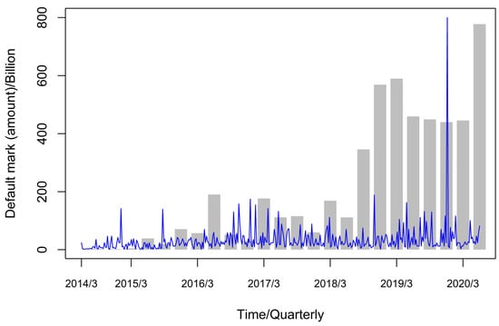
Figure 1. Trend graph of quarterly cumulative default amount (bar) and daily default amount.

7.1. Model Variable Study

From Figure 2, the average default intensity arrival rate (day) fluctuates in the interval [0, 25]. Due to the distribution of the average default arrival rate exhibiting characteristics similar to a normal distribution, it is reasonable to assume that there is an unobserved systematic risk factor $Z_t$ that affects the average default event rate that can be fitted by the geometric Brownian motion $W_t$ under a random walk scale. The results of the J-B test on the true value of the average intensity of financial default arrival parameter ${\lambda }_t$ show that p-value $<0.05$, indicating that the series test of the average arrival times of default rejects the normality hypothesis, as shown in the Table 1. Combined with the peak and thick tail shape of the average default arrival rate image, it shows that the extreme value phenomenon of the distribution of the average occurrence rate of financial default events is significant. The probability of the occurrence of financial default events is relatively high. At the same time, the influence of contagion factors is obvious in Figure 2. After the default event occurs, the probability of another default event increases. Therefore, the default event is not completely determined by the random walk scale. Under the Brownian motion $W_t$ interpretation, there is also a strong contagion factor.

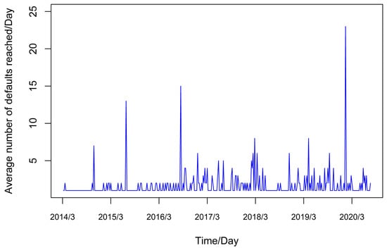
Figure 2. Trend of the average number of default arrivals.

Table 1. J-B test result.

	Value
Skew	6.78
Kurtosis	66.84
Jarque–Bera	67,966.17
p-value	0.00

In Figure 3, the solid line depicts quarterly GDP statistics, whereas the dotted line depicts quarterly average default arrivals. The link between GDP and the quarterly average default arrival rate reveals a p-value of 0.05, as shown in the Table 2. As a result, it seems appropriate to include GDP, a partially observable quantity, in the explanation of the intensity parameter model, implying that the macro-financial environment has a greater impact on the financial default arrival rate. The macroeconomic environment substantially impacts the pace at which financial defaults arrive. It can be utilized to fit the underlying pattern features of changes in the intensity parameter. Defaults tend to climb in tandem with the general financial environment’s volume, but the average growth rate of defaults is more moderate or even declining.

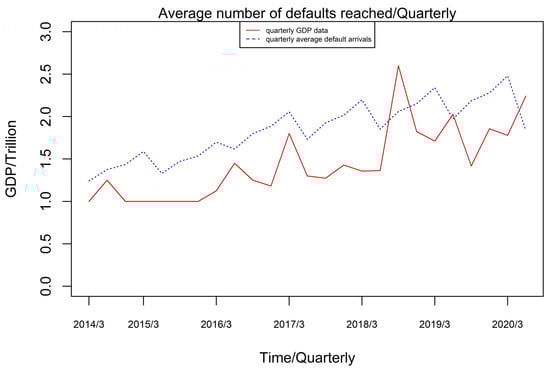
Figure 3. Average default arrivals (quarterly) vs. GDP data (quarterly) trend graph.

Table 2. Results of the correlation test between GDP and quarterly average default arrival rate.

	Value
t	3.98
df	23
p-value	0.00
cor	0.64

Figure 4 shows that when a contagion event occurs, the default amount $U_n$ (dashed line) and the average daily default arrivals (solid line) have a fairly consistent trend and periodicity. Therefore, it is reasonable to use $log{U}_n$ to build a Hawkes model that simulates the effect of the contagion factor on the average default arrival rate at the random travel scale using a model with the half-decayed self-excitation effect. Although the self-excited effect accounts for a small proportion of the model description, at moment T when the contagion effect causes extreme marker values, the self-excited term can better describe the fluctuation of the average default arrival rate affected by infectious factors. Thus, the setting of the self-excited term can better describe the model in extreme value situations.

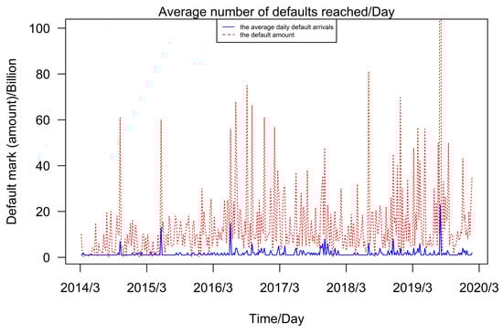
Figure 4. Default marker (amount) vs. average default arrival rate trend.

7.2. Comparative Analysis of the Model

The filtered likelihood algorithm is used to estimate the parameters of the model. Compared with the Monte Carlo method, the filtered likelihood algorithm greatly reduces the computational burden of estimating the a posteriori mean of the intensity parameter likelihood function; compared with the EM algorithm, the filtered likelihood algorithm enhances the efficiency of parameter estimation without increasing the estimation error so that the model can converge better and has a better fit. The parameters are $\theta =\left[{\alpha }_1,{\alpha }_2,{\alpha }_3,{\alpha }_4,{\gamma }_1,{\gamma }_2,{\gamma }_3,{\gamma }_4,{\gamma }_5,{\gamma }_6\right]$. Since the unobservable variable $Z_t$ in the second model is inscribed by a random variable whose conditional probability distribution is log-normal with respect to its transfer probability, the logarithmization of this variable yields its mean ${\gamma }_5\left({\tau }^j-{\tau }^{j-1}\right)$ and standard deviation ${\gamma }_6\sqrt{{\tau }^j-{\tau }^{j-1}}$ at each fixed interval ${\tau }^j-{\tau }^{j-1}$. In the case where the state is $Z^{l^z}$ at moment ${\tau }^{j-1}$ is known, the next moment state is the transfer probability obtained by integrating over all states of $\frac{u}{Z^{l^z}}$ as shown in (44):

$${\mathrm{P}}_{\theta }\left[Z_{{\tau }^j}\in {\mathrm{A}}_z^{k_z}\mid Z_{{\tau }^j}=z^{l_z}\right]={\int }_{{\mathrm{A}}_z^{k_z}\mid }\frac{1}{u}\varphi \left(log\frac{u}{z^{l_z}};{\gamma }_5\left({\tau }^j-{\tau }^{j-1}\right),{\gamma }_6\sqrt{{\tau }^j-{\tau }^{j-1}}\right)du$$

(44)

where $\varphi (\ast ;a,b)$ is a normally distributed probability density function with mean a and standard deviation b, and $A_z^{k_z}$ is a subinterval after partitioning the $Z_t$ state space. Also, after we analyze the unobservable variables of the first model, it is evident that since the factors set in the first model to capture the variables of systematic risk are standard mean-reverting CIR models, the initial values of the model are set to obey, and the shape parameter $\frac{2kz}{{\sigma }^2}$ is a non-centered chi-square distribution with scale parameter $\frac{{\sigma }^2}{2k}$. Meanwhile, it is easy to know through a calculation that its initial values can be set to the shape parameter $v=4.111$ and scale parameter $\lambda =0.497$. Therefore, with the conditional transfer probability under time division $m^T$, state division $m^s$ can be calculated by Equation (45):

$$p_{\theta }(t,y\mid 0,x)=c{e}^{-u-v}{\left(\frac{u}{v}\right)}^{q/2}{I}_q\left(2\sqrt{uv}\right),x,y\in R_{+},$$

(45)

where, for parameters, c is $\frac{2k}{{\sigma }^2\left(1-e^{-kt}\right)}$ and q is $\frac{2kz}{{\sigma }^2}-1$; for variables, u is $cx{e}^{-kt}$ and v is $cy$; and $I_q\left(x\right)$ is the q-order first class modified Sebel function ${\sum }_{i=0}^{\infty }{\left(\frac{x}{2}\right)}^{2i+q}\frac{1}{i!\Gamma (i+q+1)}$.

The asymptotic estimation of the intensity parameter likelihood function using the filtered likelihood algorithm and the locally optimal parameter estimation of the second model, and the first model likelihood function obtained by the simplex method, as shown in Table 3. For the design of the initial values of the model, on the one hand, we refer to the relevant literature, and on the other hand, we consider the weight of the parameters in the model. For example, parameters ${\gamma }_5$ and ${\gamma }_6$ of the latent variable $Z_t$ in the first model are set to consider the variation of $Z_t$ per unit time t and the variation of Brownian motion $W_t$ relative to $Z_t$ at each moment, respectively. From the analysis of the parameters, we can see that the contagious factor $X_t$ and the unobservable latent variable $Z_t$ have a positive influence on the model but the proportion is relatively small, while the partially observable explanatory variable $Y_t$ has a positive influence on the model by decaying the period with a relatively large proportion.

Table 3. Financial default model parameter estimation.

Parameter	The First Model Initial Value	The First Model Parameter Estimation	The Second Model Initial Value	The Second Model Parameter Estimation
${\alpha }_1$	4.0	3.0	3.0	3.0
${\alpha }_2$	3.0	3.0	3.0	3.0
${\alpha }_3$	2.0	2.0	2.0	2.0
${\alpha }_4$	0.2	2.5	2.5	−0.125
${\gamma }_1$	0.5	−0.5	−0.5	0.5
${\gamma }_2$	2.0	1.5	1.0	0.2
${\gamma }_3$	1.0	0	0.2	5.0
${\gamma }_4$	4.0	5.0	5.0	0.2
${\gamma }_5$	−0.5	−0.125	−0.125	0.4
${\gamma }_6$	0.53	0.5	0.5	0.32

The right panel of Figure 5 shows the fit of the second model to the average default arrival rate. The figure shows that the second model better describes the overall trend of the average default arrival rate and has a better fit for the contagion factors of default events. The left panel of Figure 5 shows the fit of the first model to the average default arrival rate. It can be seen that the first model reflects the overall trend of the average default arrival rate better than the second model. The first model has a better fit for the “spikes thick tail” of the default arrival rate distribution because it takes into account the influence of the contagion factors depicted by the Hawkes model represented by $e^{-\kappa \left(t-T_n\right)log{U}_n}$. The fit also matches the moment of default, the change in decay and the magnitude of the event. Combined with the higher values of the coefficient of determination $R^2$ and AIC of the first model, it can be concluded that the first model is a better fit for the stochastic average default intensity arrival rate of financial default events in China in the case of small samples, as shown in the Table 4.

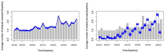
Figure 5. Default marker (amount) vs. average default arrival rate trend.

Table 4. Comparison of financial default model values.

	The First Model	The Second Model
AIC	785	744
BIC	776	753
$R^2$	0.108	0.325
MLE	503	396

8. Conclusions and Recommendations

From a macro perspective, financial default data can indicate the stability and risk level of the national financial environment. The timing of financial defaults and the regularity of the accumulated default amount can be used as a benchmark for the stability and future predictions of the financial market’s development. Two default intensity parameters models are investigated in this paper. Because the first model accounts for the self-excitation impact of cluster default factors, it does not overstate the influence of latent variables on the model and hence has a better fit for small samples of data, such as China’s bond default market. In this paper, we estimate the default intensity parameters in these two models based on the filtered likelihood method with great likelihood, which enhances the interpretation of the parameter solution and the efficiency of the model parameter solution, and, to some extent, reduces the estimation errors caused by the nature of the filtered likelihood method [27]. The default intensity model can be improved in the future study by selecting relevant explanatory factors that are more appropriate for China’s national conditions, allowing it to play a stronger role in the early warning and prediction of China’s financial default market.

References

- Shreve, S. Stochastic Calculus for Finance-Continuous Times Models; Springer: New York, NY, USA, 2003; pp. 125–251. [Google Scholar]
- Bremnud, P. Point Process and Queues-Martingale Dynamics; Springer: New York, NY, USA, 1980; pp. 150–233. [Google Scholar]
- Gordy, M.B. A Risk-Factor Model Foundation for Ratings-Based Bank Capital Rules. Journey Financ. Intermediat. 2003, 12, 199–232. [Google Scholar] [CrossRef]
- Das, S.; Duffie, D.; Kapadia, N.; Saita, L. Common Failings: How Corporate Defaults are Correlated. J. Financ. 2006, 62, 93–117. [Google Scholar] [CrossRef]
- Duffie, D.; Saita, L.; Wang, K. Multi-period corporate default prediction with stochastic covariates. J. Financ. Econ. 2007, 83, 635–665. [Google Scholar] [CrossRef]
- Azizpour, S.; Giesecke, K.; Schwenkler, G. Exploring the sources of default Clustering. J. Financ. Econ. 2018, 129, 154–183. [Google Scholar] [CrossRef]
- Hawkes, A.G. Spectra of some self-exciting and mutually exciting point processes. Biometrika 1971, 58, 83–90. [Google Scholar] [CrossRef]
- Chen, Y.S.; Zou, H.W.; Cai, L.X. Credit Default Swap Pricing Based on Supply Chain Default Transmission. South China Financ. 2018, 8, 33–42. [Google Scholar]
- Wang, X.; Hou, S.; Shen, J. Default clustering of the nonfinancial sector and systemic risk: Evidence from China. Econ. Model. 2021, 96, 196–208. [Google Scholar] [CrossRef]
- Li, C.; Ma, Y.; Xiao, W.L. Pricing defaultable bonds under Hawkes jump-diffusion processes. Financ. Res. Lett. 2022, 47, 102738. [Google Scholar]
- Xing, K.; Luo, D.; Liu, L. Macroeconomic conditions, corporate default, and default clustering. Econ. Model. 2023, 118, 106079. [Google Scholar] [CrossRef]
- Ogata, Y. The Asymptotic Behavior Of MaxiumLikehood Estimators for Stationary Point Processes. Ann. Inst. Stat. Math. 1978, 30, 243–261. [Google Scholar] [CrossRef]
- Fernando, B.P.W.; Sritharan, S.S. Nonlinear Filtering of Stochastic Navier-Stokes Equation with Ito-Levy Noise. Stoch. Anal. Appl. 2013, 31, 381–426. [Google Scholar] [CrossRef]
- Lando, D. On Cox Processes and Credit Risky Securities. Rev. Deriv. Res. 1998, 2, 99–120. [Google Scholar] [CrossRef]
- Elliott, R.J.; Chuin, C.; Siu, T.K. The Discretization Filter: On filtering and estimation of a threshold stochastic volatility model. Appl. Math. Comput. 2011, 218, 61–75. [Google Scholar]
- Giesecke, K.; Schwenkler, G. Filtered likelihood for point processes. J. Econom. 2018, 204, 33–53. [Google Scholar] [CrossRef]
- Gourieroux, C.; Monfort, A.; Mouabbi, S.; Renne, J.P. Disastrous defaults. Rev. Financ. 2021, 25, 1727–1772. [Google Scholar] [CrossRef]
- Duffie, D.; Eckner, A.; Horel, G. Frailty Correlated Default. J. Financ. 2009, 64, 2089–2123. [Google Scholar] [CrossRef]
- Chakrabarty, B.; Zhang, G. Credit contagion channels: Market microstructure evidence from Lehman Brothers’ bankruptcy. Financ. Manag. 2012, 41, 320–343. [Google Scholar] [CrossRef]
- Collin-Dufresn, P.; Goldstein, R.S.; Martin, J.S. The Determinants of Credit Spread Changes. J. Financ. 2001, 68, 2177–2207. [Google Scholar] [CrossRef]
- Liu, X.D.; Jin, X.J. Parameter estimation via regime switching model for high frequency data. J. Shenzhen Univ. (Sci. Eng.) 2018, 35, 432–440. [Google Scholar] [CrossRef]
- Liu, X.D.; Wang, X.R. Semi-Markov regime switching interest rate term structure models—Based on minimal Tsallis entropy martingale measure. Syst. Eng.-Theory Pract. 2017, 37, 1136–1143. [Google Scholar]
- Xu, Y.X.; Wang, H.W.; Zhang, X. Application of EM algorithm to eatimate hyper parameters of the random parameters of Wiener process. Syst. Eng. Electron. 2015, 37, 707–712. [Google Scholar]
- Giesecke, K.; Schwenkler, G. Simulated likelihood estimators for discretely observed jump–diffusions. J. Econom. 2019, 213, 297–320. [Google Scholar] [CrossRef]
- Duffie, D.; Pan, J.; Singleton, K.J. Transform Analysis and Asset Pricing for Affine Jump-diffusions. Econometrica 2000, 68, 1343–1376. [Google Scholar] [CrossRef]
- Hou, Z.T.; Ma, Y.; Liu, L. Estimation of the stationary distribution parameters based on the forward equation. Acta Math. Sci. 2016, 36, 997–1009. [Google Scholar]
- Wang, S.W.; Wen, C.L. The Wavelet Packet Maximum Likelihood Estimation Method of Long Memory Process Parameters. J. Henan Univ. (Nat. Sci.) 2006, 2, 79–84. [Google Scholar]
Disclaimer/Publisher’s Note: The statements, opinions and data contained in all publications are solely those of the individual author(s) and contributor(s) and not of MDPI and/or the editor(s). MDPI and/or the editor(s) disclaim responsibility for any injury to people or property resulting from any ideas, methods, instructions or products referred to in the content. |
© 2023 by the authors. Licensee MDPI, Basel, Switzerland. This article is an open access article distributed under the terms and conditions of the Creative Commons Attribution (CC BY) license (https://creativecommons.org/licenses/by/4.0/).