Abstract
Traffic incidents pose substantial hazards to public safety and wellbeing, and accurately estimating their duration is pivotal for efficient resource allocation, emergency response, and traffic management. However, existing research often faces limitations in terms of limited datasets, and struggles to achieve satisfactory results in both prediction accuracy and interpretability. This paper established a novel prediction model of traffic incident duration by utilizing a tabular network-TabNet model, while also investigating its interpretability. The study incorporates various novel aspects. It encompasses an extensive temporal and spatial scope by incorporating six years of traffic safety big data from Tianjin, China. The TabNet model aligns well with the tabular incident data, and exhibits a robust predictive performance. The model achieves a mean absolute error (MAE) of 17.04 min and root mean squared error (RMSE) of 22.01 min, which outperforms other alternative models. Furthermore, by leveraging the interpretability of TabNet, the paper ranks the key factors that significantly influence incident duration and conducts further analysis. The findings emphasize that road type, casualties, weather conditions (particularly overcast), and the number of motor and non-motor vehicles are the most influential factors. The result provides valuable insights for traffic authorities, thus improving the efficiency and effectiveness of traffic management strategies.
MSC:
68T07; 00A69
1. Introduction
Traffic incidents are a major cause of delays and congestion in the road network. They can also lead to accidents, injuries, and fatalities [1,2]. The duration of a traffic incident can vary widely, depending on the type of incident, the severity of the damage, and the resources available to clear the scene. The ability to accurately predict the duration of a traffic incident would be beneficial for a number of reasons. First, it would allow traffic managers to better plan for and respond to incidents. This could help to reduce delays and congestion, and it could also help to improve safety. Second, it would allow drivers to make informed decisions about their travel plans. This could help them to avoid congested areas and to arrive at their destinations on time.
The term “duration” in the context of a traffic incident refers to the overall time period starting from when the incident takes place until the arrival of traffic police at the scene and the completion of handling. Generally, the duration of a traffic incident can be divided into the following stages [3], as illustrated in Figure 1 below.
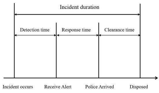
Figure 1.
Stages of a traffic incident.
Generally, the duration of a traffic incident can be divided into three stages: detection time, response time, and clearance time. Their specific meanings are as follows: (1) Detection time: The time from the occurrence of the incident to when traffic police or other management personnel discover it. The incident can be detected through means such as surveillance videos and emergency calls to the police hotline (e.g., 122 in China). This process allows relevant personnel to confirm the occurrence of the incident. (2) Response time: The time from confirming the occurrence of the incident to the arrival of traffic police and other emergency personnel at the scene. (3) Clearance time: The time during that traffic police and other emergency personnel work at the scene, such as conducting investigations, providing medical assistance to injured individuals, and removing debris. This process often involves traffic control measures, such as lane closures, until the measures are revoked.
The duration of a traffic incident is determined by the cumulative time of three distinct periods, encompassing the time from the incident’s initiation to its complete resolution. The length of this process is influenced by various factors. For example, rapid incident detection, efficient management, and a well-established emergency response system contribute to reducing the duration of the incident. Some studies also include the time required for traffic flow to fully recover after incident clearance as part of the duration. This additional time is mainly influenced by the traffic conditions at the time of the incident and uncontrollable environmental factors, such as congestion, the number of occupied lanes, and weather conditions. For simplicity, this study only considers the first three time periods.
There has been a growing body of research on the prediction of traffic incident duration. A number of different methods have been proposed, mainly including statistical models and machine learning models [4,5]. The main methods and characteristics of these approaches are summarized in Table 1.
Statistical Approach
Statistical models are representative predictive methods in traffic incident duration analysis. Such models are based on the assumption that the duration of a traffic incident can be predicted by a set of factors, including the incident type, time of day, and prevailing weather conditions, as well as the traffic volume. These models encompass widely used regression models [6,7,8,9,10], probabilistic statistical models [11,12,13], hazard-based models [14,15,16,17,18], copula-based models [19], finite mixture models [20,21], etc. They typically assume that the data follow a certain distribution and model and predict the distribution of the data. For example, Valenti, G. and Lelli, M. [6] conducted an analysis using a multivariate linear regression model to study six major factors, including the presence of on-site emergency measures, involvement of heavy vehicles, occurrence during peak traffic hours, extent of damage to traffic facilities, number of lanes, and the occurrence of fire. The study revealed that for certain specific incidents, as the duration of the incident response increased, the regression errors also increased. Similarly, there have been advancements in linear regression, such as the development of quantile analysis [22,23], which have been applied successfully in incident duration.
Machine Learning Approach
Machine learning models are based on the idea that the duration of a traffic incident can be predicted by learning from historical data [4]. Machine learning models can be trained on datasets that include information about the type of incident, time of day, weather conditions, traffic volume, and duration of the incident. Typical machine learning models include K-nearest neighbor (KNN) [15], support vector machine (SVM) [24], annual neural network (ANN) [25], decision tree (DT) [26], and random forest (RF) [27,28], which can be categorized into three types—distance metric learning, ensemble learning, and neural network learning. Table 1 summarizes the characteristics and differences of various types of methods. For example, SVM is a supervised learning algorithm that can be used to classify or predict data. Another machine learning model for predicting traffic incident duration is the random forest algorithm, which is an ensemble learning algorithm that combines the predictions of multiple decision trees. Decision trees are a type of supervised learning algorithm that can be used to classify or predict data [29]. Decision trees work by splitting the data into smaller and smaller groups until each group contains only data points of the same class. Deep neural networks are a type of machine learning model that can learn complex relationships between variables. Deep neural networks can be used to predict the duration of a traffic incident by considering a large number of variables, such as the type of incident, time of day, weather conditions, traffic volume, and surrounding environment. Some models combine the strengths of statistical models and machine learning models. Hybrid models [3,27,30] can be more accurate than either statistical models or machine learning models alone. One example of a hybrid model is the Bayesian network [31]. Bayesian networks, also known as Bayesian belief networks or graphical probabilistic models, are graphical models that depict the probabilistic relationships between variables. Bayesian networks can be used to predict the duration of a traffic incident by considering the relationships between the type of incident, time of day, weather conditions, traffic volume, and duration of the incident [32,33].

Table 1.
Summary of the main research methods.
Table 1.
Summary of the main research methods.
| Research Approach | Typical Methods | Description |
|---|---|---|
| Statistical Approach | Hazard-based models [14,15,16,17,18], Quantile regression [22,23], Copula-based approach [19], and Finite mixture models [20,21] | Statistical methods attempt to establish models to explain various influencing factors. The main differences lie in the model construction and the choice of parameter estimation methods. |
| Machine Learning Approach | Distance Metric Learning (1) KNN [15] (2) SVM [24] | KNN and SVM both use distance metrics to measure the similarity between instances. The goal of KNN is to find the optimal classifier by minimizing the classification error, while SVM aims to find the hyperplane that maximizes the margin between classes for better classification performance. |
| Ensemble Learning (1) RF [27,28] (2) GBDT [34] | RF and gradient boost decision tree (GBDT) both combine multiple decision trees to make predictions. Specifically, RF builds independent trees through random feature selection and voting, while GBDT sequentially builds trees to correct the residuals of previous trees. | |
| Neural Network Learning (1) Bayesian Neural Network [31] (2) ANN [25] | Neural Network Learning utilizes network architectures for predicting incident duration. Bayesian neural networks incorporate Bayesian inference techniques to model and quantify uncertainty in the network’s predictions, while ANN typically focuses on optimizing network weights through backpropagation without explicitly considering uncertainty. |
The existing research on traffic incident duration prediction has made significant progress; however, several research gaps remain to be addressed. This literature review highlights the following key research gaps:
(1) Limited dataset coverage: Previous studies often suffer from limitations in dataset size, temporal and spatial coverage, and the variety of incident and road types included. To overcome this gap, there is a need for larger-scale datasets that encompass a broader range of road types, such as urban roads, highways, and expressways, and that include diverse influencing factors.
(2) Prediction accuracy of statistical model: Traditional decision tree and statistical models have been widely used for their interpretability in predicting traffic incident duration. However, these models often have limitations in terms of prediction accuracy, especially when dealing with complex relationships among features.
(3) Interpretability of deep learning models: Deep learning models have gained popularity in various domains, but may not directly translate to traffic tabular datasets. One challenge is the reduced interpretability of deep learning models, making it difficult to analyze feature importance and understand the decision-making process at the individual data point level in the context of traffic incident duration prediction.
Based on the analysis above, we need to find a suitable predictive model for traffic incident data and apply it to the analysis of traffic incident data on complex road networks in large cities. As most of the traffic incident data are in tabular format, our model should have good adaptability to tabular data, whether categorical or numerical. Additionally, we aim for both high prediction accuracy and interpretability. This is because traffic incidents are influenced by multiple factors, making accurate prediction of incident duration challenging, and we also want to conduct in-depth analysis of the factors affecting incident duration. Fortunately, the TabNet [35] model meets our requirements. TabNet is a particular deep learning model specifically designed for tabular data analysis, which aligns well with the nature of our problem. It leverages sequential attention to dynamically select a subset of relevant features at each stage of decision making. This feature selection mechanism allows the model to focus its learning capacity on the most informative and meaningful features in the dataset. By selecting important features, TabNet improves the model’s interpretability and ability to capture complex patterns in the data [35]. Moreover, previous studies have demonstrated favorable outcomes in both predictive accuracy and interpretability [36,37]. Therefore, in this study, we adopt the TabNet model to predict the duration of incidents on diverse road types in large cities, aiming to improve prediction accuracy and uncover the key factors influencing duration, ultimately providing insights for intelligent traffic management.
The present study introduces several notable contributions to the field of predicting traffic incident duration. Firstly, it addresses the data limitations of previous research by utilizing a more extensive dataset that spans six years and covers the entire city of Tianjin, China. This dataset encompasses a wide range of incident types and diverse regions, allowing for a comprehensive analysis of influential factors. Secondly, to achieve a balance between interpretability and predictive accuracy, the research adopts the TabNet model, which leverages the advantages of deep learning while maintaining interpretability. This model facilitates the examination of the significance of various influencing factors. Lastly, the analysis of the factors influencing incident duration provides valuable insights for intelligent traffic management, enabling optimized resource allocation and more efficient incident management, ultimately improving overall traffic flow and system effectiveness.
The rest of this paper is structured as follows. Section 2 presents a comprehensive overview of the main principles of the employed and alternative models in our study. Section 3 presents a comprehensive analysis of the dataset used in this research. In Section 4, we analyze the experimental results obtained from the employed model. Subsequently, we focus on the interpretability of experiment results in Section 5 by examining the overall feature importance and investigating the step-wise feature selection process. Section 6 concludes this paper.
2. Model Principals
The perceptron is the foundation of the neural network, while deep neural networks (DNNs) are neural networks with multiple hidden layers. DNNs have demonstrated remarkable success in image analysis, text processing, and audio recognition. However, traditional DNN architectures, such as those based on convolutional layers or multi-layer perceptrons (MLPs), are not well-suited for tabular data. These architectures often have excessive parameters and lack the necessary inductive bias to capture the decision manifold in tabular data. On the other hand, decision trees and their variants heavily rely on feature engineering, which poses a significant limitation. In contrast, TabNet model is a deep learning model that combines the benefits of deep neural networks with interpretability in tabular data analysis. Below is the detailed model description.
2.1. Structure of TabNet Model
TabNet, originally proposed by Sercu [35], has gained popularity for its effective handling of tabular data and for the provision of feature importance rankings. It consists of a shared feature transformer, decision steps, and an adaptive feature selection mechanism [36]. The model follows an encoder–decoder structure, where the encoder captures relevant features and the decoder utilizes them for prediction. TabNet’s interpretability and prediction accuracy have made it a suitable choice for various tasks, including predicting traffic incident durations.
In Figure 2, the TabNet encoder architecture is depicted. The structure of TabNet is a multi-step process that includes the transformation and masking of features. It works with both numerical and transformed categorical data from tabular datasets. An attention mechanism influences how the features contribute to each step, taking the preceding step’s outcome into account. This mechanism manipulates the features at each step, and these transformed features are then integrated into the overall decision-making process.

Figure 2.
TabNet encoder architecture.
2.1.1. Feature Selection
The TabNet model achieves feature selection through the Mask module at each decision step. The attentive transformer within each step determines the specific function to be applied. Figure 3 illustrates how the Attentive transformer learns a mask for the feature selection process in the current decision step . The specific meanings are as follows [36]:

Figure 3.
Attentive transformer.
(1) The split module splits the tensor output from the feature transformer layer into two parts. This process can be represented by equation , where is used to compute the final output of the model and is used to calculate the mask layer for the next step.
(2) is reserved and passed to the following flows.
(3) means that undergoes the fully connected layer (FC layer) to extract more abstract features and the batch normalization layer (BN layer) to stabilize training and reduce sensitivity to initialization.
(4) is then scaled by , which is the scale of the previous decision step. denotes the degree of feature usage in earlier steps. The mathematical representation can be stated as: .
(5) The resulting is generated through the Sparsemax function, as depicted by M [i] = Sparsemax(s [i]).
Sparsemax is a technique that encourages sparsity by mapping the Euclidean projection onto the probabilistic simplex. This mapping aids in achieving sparser feature selection by promoting a more concentrated distribution of probabilities. It ensures that the sum of the feature selection weights, denoted as , for each sample and feature , equals 1, where represents the feature dimension. By implementing a weight distribution for each feature of each sample, Sparsemax enables instance-wise feature selection. This allows TabNet to focus on the most informative features in each decision step. To regulate the sparsity level, TabNet incorporates a regularization term. This term is defined as follows:
When a significant portion of features in a dataset exhibit redundancy, the introduction of sparsity in feature selection can offer a more effective inductive bias, leading to improved convergence and higher accuracy levels.
(6) The update of in is carried out using Equation (2). When the parameter is set to 1, this indicates that each feature is allowed to appear in only one decision step.
(7) The feature selection of the current decision step is achieved by multiplying with the feature elements. After selecting the relevant features, they are then fed into the current step’s feature transformer and become ready for a new loop.
2.1.2. Feature Processing
The initial input to the feature transformer in Figure 4 is the combination of the original features (for the initial step) or the masked features (for the subsequent steps) and the output from the prior decision step. This transformed input undergoes a series of transformations in the feature transformer to learn more complex, abstract features. The feature transformer has two types of transformation blocks: shared blocks and independent blocks. Each block is composed of a succession of transformations, including a fully connected (FC) layer, a normalization (typically Ghost Batch Normalization), and a gated linear unit (GLU) layer.

Figure 4.
Feature transformer.
- (1)
- Shared blocks: The weights of the shared blocks are shared across all decision steps. This means that the transformations applied in the shared blocks are identical for every decision step. Shared blocks are designed to extract common patterns from the input features, which are useful across all decision steps, aiding in model generalization and reducing the number of parameters.
- (2)
- Independent blocks: Conversely, the independent blocks have weights that are independent for each decision step. This means that for each decision step, the transformations applied in these blocks can be different. Independent blocks allow each decision step to learn and extract different features or representations from the transformed output of the shared blocks. This design supports the model’s ability to capture complex interactions and relationships.
2.1.3. TabNet Decoder Architecture
In Figure 5, the TabNet decoder begins its operation with the encoded representation, which is the cumulative sum of all of the decision step outputs from the encoder, excluding their subsequent passage through the FC layer. This condensed encoded representation is then fed into the decoder. To decode the embedded information, the feature transformer is employed, which is capable of transforming the encoded representation back into a feature space. This transformation process is not carried out in a single step, but rather is accomplished across multiple steps. The final output from the decoder is the reconstructed feature, which is the result of these multiple transformation steps.
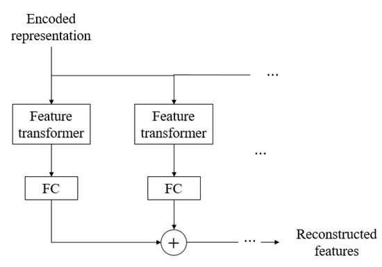
Figure 5.
TabNet decoder architecture.
2.2. Interpretability of TabNet Model
The TabNet model employs the concepts of a mask matrix and an importance matrix in the process of feature selection. These matrices are the result of an attention mechanism within each decision step, which prioritizes certain features over others by assigning unique weights. The mask matrix captures the immediate importance of features in each decision step, while the importance matrix cumulates these weights over all decision steps to create an aggregated importance score. This combined score allows TabNet to effectively identify and prioritize features that have the greatest influence on the model’s output, enhancing the overall interpretability of the model. The following is a detailed explanation:
Mask Matrix
The mask matrix in TabNet determines the relevance of each feature during the decision-making process. It is created using a sparsity-inducing regularization technique known as the “sparsemax” function, as stated in Equation (1). The mask matrix, denoted by , is a binary matrix of the same shape as the input features . Each element of the mask matrix indicates whether feature is considered relevant for predicting the output of data point . The mask matrix effectively identifies the important features by assigning high weights (close to 1) to the relevant features and low weights (close to 0) to the irrelevant ones. By visualizing or analyzing the mask matrix, researchers and practitioners can understand which features are crucial for the model’s predictions.
Importance Matrix
The importance matrix in TabNet quantifies the relative importance of each feature based on its contribution to the model’s predictions. It is calculated by considering the average of feature importance scores across different decision steps. The importance matrix, denoted by , has the same shape as the input features , with each element indicating the importance of feature for predicting the data point . The Mathematical expression is
Here, represents the mask matrix at the -th decision step, denotes the learnable weight matrix associated with the -th decision step, and the sum (∑) is taken over all of the decision steps. The importance matrix provides a comprehensive view of feature importance throughout the model’s decision process. By analyzing the importance matrix, we can gain insights into the relative influence of each feature on the final predictions, allowing for a better understanding of the model’s behavior and interpretability.
In summary, the mask matrix and importance matrix in the TabNet model contribute to its interpretability. The mask matrix identifies relevant features for prediction, while the importance matrix quantifies the importance of each feature. These matrices enable us to analyze and explain the decision-making process, facilitating a deeper understanding of the model’s behavior and aiding in the interpretation of its predictions.
2.3. Alternative Models for Contrast
This study considers the following popular prediction models as reference models for the Tabnet model.
(1) Ridge Linear Regression (RLR):
RLR is an extension of ordinary least squares regression that addresses multicollinearity issues. The model is represented by equation , where is the dependent variable, is the matrix of predictors, is the coefficient vector, and is the error term. The goal of RLR is to estimate the optimal values of that minimize the objective function . Here, is the regularization parameter that controls the amount of shrinkage applied to the coefficients. The term represents the L2 norm of the coefficient vector, penalizing large coefficients. By balancing the residual sum of squares and the constraint on coefficients, RLR improves model generalization by reducing the impact of collinear predictors.
(2) Decision Tree (DT):
DT is a non-parametric supervised learning method that uses a tree-like structure to make predictions [29]. It partitions the data based on the values of the predictors and creates decision rules to classify or predict the response variable.
(3) Support Vector Regression (SVR):
SVR is a regression method that utilizes the principles of support vector machines. It aims to find the optimal hyperplane that maximizes the margin while minimizing the error between the predicted and actual values. SVR assumes that the dependent variable y is expressed as , where is a feature mapping function that transforms the input data into a higher-dimensional space. The mathematical goal can be expressed as follows:
(4) Artificial Neural Network (ANN):
ANN is a machine learning model inspired by the structure and function of biological neural networks [38,39]. It consists of interconnected nodes (neurons) organized in layers. ANN can learn complex patterns and relationships through a process called training, which involves adjusting the weights and biases of the connections between neurons. The optimization objective can be defined as follows:
where are the corresponding parameters. is the hyper penalty coefficient.
(5) Random Forest (RF):
RF is an ensemble learning method that combines multiple decision trees to make predictions [40,41]. Each tree in the forest is trained on a random subset of the data, and the final prediction is determined by aggregating the predictions of individual trees. RF is known for its ability to handle high-dimensional datasets and capture complex interactions among variables.
3. Dataset Description
3.1. General Summary
The selected traffic incident data for this section were obtained from the Traffic Management Department of Tianjin City. The data cover the period from 1 January 2009 to 31 December 2015, and includes approximately 31,000 incident records. The dataset covers various road types, including highways, urban expressways, urban arterial roads, and other ordinary or minor roads. Every data record covers various attributes, and after removing irrelevant fields such as identifiers, the remaining fields can be categorized into the following four groups:
Time and location of occurrence: This includes fields such as “administrative district”, “time of happening”, “time of start investigation”, “time of ending investigation, and “day of the week”.
Infrastructure conditions: This includes fields related to the road infrastructure, such as “road surface structure”, “road conditions”, “lane configuration”, “intersection type”, and “road type”.
Environmental conditions at the scene: This includes fields such as “weather”, “topography”, and “lighting conditions”.
Severity of the incident: This includes fields related to the severity of the incident, such as “incident type”, “collision type”, “number (#) of motor vehicles”, and “number (#) of non-motor vehicles”.
Among the mentioned incident attributes, some are numerical variables, such as “number of motor vehicles” and “number of non-motor vehicles“. Most of the others are categorical variables. For example, “administrative district” is categorized based on the primary administrative areas, “lane configuration“ is divided into mixed and one-way configurations, “road condition” is categorized as wet or flooded, “road surface structure” is classified as asphalt or cement, “intersection type” includes options such as T-junction or four-way intersection, “road type” can be categorized as expressway or highway, etc., “collision type” includes options such as head-on collision or opposite sides scraping, “topography” can be plain or mountainous, and “lighting conditions” can be daylight or illuminated at night. Finally, “incident type” includes categories such as fatal, injury, and property damage incidents. In our study, the incident duration is calculated as follows:
In actual situations, there is a certain deviation between the calculation results of Equation (6) and the strict definition in Figure 1. This is mainly because the incident investigation may not always take place at the incident scene, and after the incident is cleared, traffic management personnel may not record the incident in a timely manner. As a result, the calculated duration of certain small-scale incidents based on Equation (6) can reach several tens of hours, which clearly does not align with the actual situation. After calculation, the average value of is 56.5 min. Considering that the majority of incidents can be resolved within 1 h, this paper removes abnormal records with T > 120 min.
Note that the TabNet model requires the input features to be numerical. Therefore, categorical features need to be appropriately preprocessed into numerical format (e.g., via one-hot encoding or embedding), which adds to the data preparation process. To ensure that these categorical variables can be appropriately included in the models, we adopted the technique of “one-hot” encoding. This technique transforms each categorical variable into multiple binary variables, commonly known as dummy variables. It is an effective way to convert categorical data into a format that can be provided to machine learning algorithms to improve their performance.
When performing “one-hot” encoding, each category value is converted into a new column, and a binary value is assigned corresponding to the presence or absence of the attribute. However, this raises an issue of multicollinearity, because the value of one variable can be easily predicted with the help of the others. Multicollinearity is a problem because it undermines the statistical significance of an independent variable. We can avoid this by setting binary variables for a variable that has categorical values. This approach is also known as dummy variable trap avoidance. For example, consider an event type variable with three categories: death, injury, and property damage. In this case, we can set two binary variables and instead of three. Here, and represent a death event, and signify an injury event, and and denotes a property damage incident. Furthermore, if a categorical variable has many categories, it is often beneficial to simplify the problem by grouping less frequent or statistically insignificant categories into a single “other” category. For instance, if , , and in Table 2 are all 0, this indicates that the weather is “other”, which represents conditions such as snow, strong winds, and foggy weather. These types of weather account for only 1% of the total occurrences. After detailed data preprocessing, the transformed variables are shown in Table 2 (numeric variables are retained as is).
Table 2.
Selected features for prediction.
Figure 6 presents a histogram depicting the frequency distribution of the incident durations. The distribution shows a pronounced concentration of incidents within the duration range of 30 to 39 min. Subsequently, as the duration increases, the frequency notably decreases. This pattern can be attributed to the fact that the majority of non-severe traffic incidents, which involve no casualties or significant property damage, are typically resolved within half an hour. In contrast, severe traffic incidents pose greater challenges in terms of management, resulting in longer durations, as well as increased heterogeneity among individual incidents. By our calculations, the mean and the standard deviation of duration are 50.36 min and 40.00 min, respectively. Moreover, the skewness value is 1.02, which suggests a positively skewed distribution, indicating that the data are inclined towards longer durations. The kurtosis value of 0.02 indicates a nearly normal distribution with a slightly flatter peak and lighter tails compared with a normal distribution.
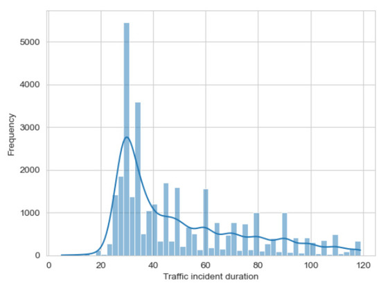
Figure 6.
Distribution of traffic incident duration.
3.2. Characteristics by Different Categories
In this section, we consider the incident duration in different categories, such as whether the incident happens in the morning or evening peak hours or whether the weather is good. Figure 7 indicates that the distribution of the incident duration is similar, regardless of whether it occurs during peak hours or non-peak hours. There could be several possible explanations for this. (a) Traffic flow: It is possible that the traffic flow during peak hours is not significantly different from non-peak hours in some areas. (b) Response time: The response time of emergency services, such as police and medical personnel, might not vary significantly between peak and non-peak hours. If the response time is consistent throughout the day, it may not contribute to a significant difference in incident duration. (c) The nature and severity of traffic incidents may not differ significantly between peak and non-peak hours, thus resulting similar incident durations. We should also note that the incident duration in our study does not include the time required for traffic flow to return to its normal state after incident clearance. Therefore, the result may change if we take the recovery time into account.

Figure 7.
Traffic incident duration (peak vs. non-peak); (a) Distribution of incident duration; (b) Box plot of incident duration.
Similarly, Figure 8 displays that the incident durations between urban (non-suburb) and suburban areas are significantly different. The average level and variance of incident duration in suburban areas are higher than those in urban areas. For example, the median incident duration in urban areas is 35 min, while it is 46 min in suburban areas. Additionally, the range of the typical distribution interval (from the 25th percentile to the 75th percentile) in suburban areas is approximately twice as wide as that in urban areas. This could be caused by the longer response times or limited resources, the road infrastructure and the geographical factors. For example, emergency services such as police and medical teams may need more time to arrive the scene, thus leading to a higher incident duration. Figure 9 reveals the traffic incident duration by incident types. It indicates that the majority of incidents involve injuries, followed by a smaller proportion of incidents involving fatalities, and an even smaller proportion involving no injuries (only property damage). Moreover, the average and variance of duration of death incidents are significantly higher than that of incidents involving only injuries, which is consistent with our intuitions, because fatal incidents typically require a more thorough investigation and documentation process. The involvement of law enforcement agencies, medical examiners, or other specialized personnel may prolong the incident duration due to the additional procedures and paperwork involved. From Figure 10, it can be seen that most incidents occurred during sunny weather conditions. Incidents that took place during overcast or rainy weather conditions had relatively longer durations compared with those during sunny weather. One possible reason is that overcast or rainy weather conditions can lead to reduced visibility, slippery road surfaces, and decreased traction, which may result in longer incident durations. Furthermore, inclement weather can cause traffic congestion due to slower driving speeds, road closures, or accidents. This congestion can delay the response time of emergency services and impede the clearance of the incident scene, leading to longer incident durations.

Figure 8.
Traffic incident durations (suburb vs. non-suburb districts); (a) Distribution of incident duration; (b) Box plot of incident duration.
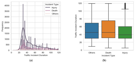
Figure 9.
Traffic incident durations (by incident type); (a) Distribution of incident duration; (b) Box plot of incident duration.
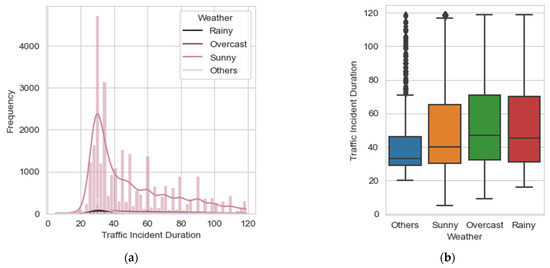
Figure 10.
Traffic incident durations (by weather); (a) Distribution of incident duration; (b) Box plot of incident duration.
We also explored the relationship between the incident duration and road types. Figure 11 displays that most incidents occurred on arterial roads, and the incident durations of arterial roads tended to be shorter. Generally, arterial roads serve as primary routes for transportation, accommodating a substantial volume of vehicles. The heavy traffic flow increases the likelihood of incidents occurring on these roads. Moreover, because of the importance and high traffic load of arterial roads, traffic police departments prioritize their monitoring and enforcement efforts in these areas. This proactive approach enables quicker detection of incidents and faster response times. On the other hand, incidents on lower-grade roads and expressways have relatively longer durations. However, this rule is not fixed, because Class-A and Class-C highways have a shorter duration than Class-B and Class-D highways, indicating the complexity of the traffic safety system. Furthermore, in Figure 12, it can be seen that a higher number of motor vehicles is associated with longer incident durations, while there is no apparent relationship between the number of non-motor vehicles and incident duration. This may be because non-motor vehicles have different characteristics and lower speeds compared with motor vehicles. As a result, incidents involving non-motor vehicles may have a different nature and require less time for resolution compared with motor-vehicle-related incidents.
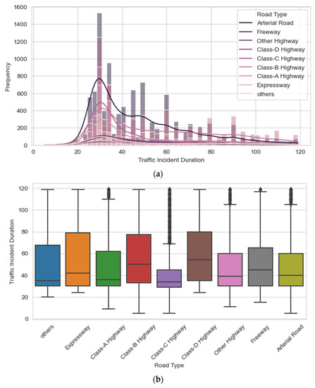
Figure 11.
Traffic incident durations (by road type); (a) Distribution of incident duration; (b) Box plot of incident duration.

Figure 12.
Traffic incident durations (by number of vehicles); (a) Motor vehicles; (b) non-Motor vehicles.
4. Experiment Results
4.1. Overall and Categorical Results
In this study, we employed multiple models, including the TabNet model, as well as other comparative models, to predict the duration of traffic incidents. We compared and evaluated the performance of these models on the entire dataset. Based on the error metrics presented in Table 3, we can summarize the performance of the models as follows: Overall, all models were capable of predicting the duration of traffic incidents to a certain extent. However, when comparing the TabNet model with the comparative models (ANN, DT, RF, RLR, and SVR), TabNet demonstrated a superior performance. Specifically, the TabNet model achieved an MAE (mean absolute error) of 17.04 min and an RMSE (root mean squared error) of 22.01 min on the full dataset. These values were lower compared with the other models, indicating that the TabNet model provided more accurate predictions of the duration of traffic incidents with smaller errors.
Table 3.
Model performance on the whole dataset.
Additionally, we examined the MAPE (mean absolute percentage error) metric, which assessed the relative error of the predictions compared with the true values. It should be noted that the MAPE values for all models, including TabNet, were relatively high (33.60%). This can be attributed to the small scale and inherent randomness and uncertainty associated with the duration of traffic incidents. However, the MAPE values obtained from the TabNet model were comparable to those reported in similar studies.
Table 4 summarizes the performance of different models in predicting the duration of traffic incidents across various categories. For example, “suburb” means the incident happened in the suburb areas, and “expressway” means the incident occurred at an expressway. As displayed in Table 4, the TabNet model performed optimally in the following categories: suburb, injury, arterial road, and peak, exhibiting lower average errors (MAE, RMSE, and MAPE) compared with the other models. It can be seen that all prediction models had higher average errors in the suburb category compared with the non-suburb category. This could be attributed to the complex nature of incidents in suburban areas, where factors such as response time, road infrastructure, population density varied, leading to higher prediction errors. Moreover, the average error was obviously higher in the death category compared with that in the injury category. The higher variability in incident durations in the death category, which may be influenced by factors such as severity of accidents, emergency response time, and medical interventions, contributed to the increased prediction errors. Similarly, the prediction error for the expressway category was higher than that for the arterial road. This could be due to the differences in traffic flow, speed limits, and incident characteristics between arterial roads and expressways. Incidents on expressways may involve higher speeds, multiple lanes, and limited access, resulting in increased complexities when predicting their durations.
Table 4.
Model performance on specific categories.
The variations in prediction errors across these categories can be attributed to the distinct characteristics and dynamics associated with different types of incidents and road environments. Factors such as traffic volume, road infrastructure, severity of incidents, and response time play crucial roles in determining the duration of incidents and contribute to the differences in prediction errors observed. Generally, TabNet’s ability to capture and model these variations to some extent resulted in a superior performance compared with other models.
4.2. Impact of Parameter Settings
To investigate the relationship between the key parameters and the prediction results, we set the main parameters as seen in Table 5. (1) TabNet: The parameter “n_step” represents the number of steps in the TabNet encoder network and was set to 1, 2, 3, 5, 7, 9, 11, 13, 15, or 17. (2) RLR: The parameter “alpha” corresponds to the regularization coefficient. It controls the amount of regularization applied to the model and we took values of 0.01, 0.05, 0.22, 1.00, 4.46, 21.54, 100, or 464.16 (in log scale). (3) DT: The parameter “n_depth” refers to the maximum depth of the decision tree. It ranged from 5 to 14, indicating the maximum number of levels the tree can grow. (4) SVR: The parameter “gamma” represents the coefficient of the RBF (radial basis function) kernel in the SVR model. It determines the influence of each training example and was set to 0.05, 0.25, 1, 6, 11, or 16. (5) ANN (artificial neural network): The “layer setting” parameter defines the architecture of the neural network. It specifies the number of layers and the nodes in each layer. The options include 10, 30, 100 (indicating one hidden layer with 10, 30, and 100 nodes, respectively); (5,5) (indicating 2 hidden layers with 5 nodes each); (10,10) (indicating two hidden layers with 10 nodes each), and (30,30) (indicating two hidden layers with 30 nodes each). (6) RF (Random Forest): The parameter “n_tree” determines the number of decision trees (estimators) in the random forest ensemble. It was set to 10, 25, 40, 55, 70, or 85 in our study.
Table 5.
Model parameter settings.
In Figure 13, we analyzed the prediction errors on the training and test sets for different models. It is evident that in most cases, the error on the test set was significantly higher than that on the training set, especially for tree-based models such as random forest and decision tree. Generally, as the parameter values increased, the complexity of the model also increased. As a result, the prediction performance on the training set tended to be better, while on the test set, it followed a pattern of initially decreasing and then increasing. This phenomenon could be attributed to overfitting, where the increased complexity led to a closer fit to the training data, but it compromised generalization to unseen data. For instance, the decision tree model showed a rapid decrease in MAE on the training set as the tree depth increased, reaching below 16 min. However, because of overfitting, the MAE on the test set increased to around 18.5 min. Similarly, the random forest model achieved an MAE of around 15 min on the training set, but exhibited a high MAE of over 18 min on the test set. It is noteworthy that the TabNet model demonstrated a consistent performance on both the training and test sets, with the MAE ranging from 17.1 min to 17.6 min across different n_step values. This indicates that the TabNet model possessed good adaptability and was less sensitive to the adjustment of training parameters, making it less prone to overfitting.

Figure 13.
Influence of the key model parameters.
5. Further Discussion
While we focused on achieving a high predictive accuracy, the ability to understand and interpret the underlying mechanisms of a model’s predictions is equally critical. Interpretability fosters trust and transparency in predictive models, and provides insights into the relationships between the input features and predictions. The TabNet model exhibits strong interpretability in the prediction process, as it allows us to assess the overall importance of explanatory variables through the “importance” metric. Additionally, the model provides insights into how features are progressively selected through the step-wise feature selection mask matrix, shedding light on the process of feature selection for prediction purposes.
More specifically, the interpretability of the TabNet model stems from its unique architecture and mechanisms. Firstly, the model employs a structured attention mechanism, where each decision step involves the selection of important features using the attention weights. By examining the importance scores assigned to different variables, we can gain a comprehensive understanding of their relative significance in the prediction process. This information enables researchers and practitioners to identify the key drivers behind the model’s predictions and to make informed decisions based on these insights. Furthermore, the step-wise feature selection mask matrix employed in TabNet provides detailed information about the sequential selection of features. It allows us to track the progression of feature inclusion or exclusion, providing a transparent view of how the model dynamically incorporates or discards features during the learning process. This level of granularity in feature selection offers valuable insights into the model’s decision-making process, enhancing its interpretability.
5.1. Numerical Feature Importance
Regarding the importance of features, based on our calculations on the entire dataset, the feature importance scores are as follows: overcast (0.273), death (0.194), number of non-motor vehicles (0.115), injury (0.112), and Class-B highway (0.09). Note that scores of all features sum up to 1, indicating the relative importance of each feature. Overall, these important features align with our previous overall description in Section 3 and exhibit good discriminatory power. For instance, “overcast” implies bad weather and poor visibility, which is supported by the comparison in Figure 10, which confirms its impact on incident duration. Moreover, the importance of the “death” feature aligns with our intuition. However, the importance of the number of non-motor vehicles may not be obvious. Although Figure 12b shows no fixed relationship between the number of non-motor vehicles and duration, the model identifies it as an important feature, indicating its potential influence in conjunction with other features on the duration.
The feature importance ranking in Figure 14 represents the model’s overall assessment on the entire dataset. However, the trained model evaluates the importance of each feature individually for each instance. Figure 15 below illustrates the average feature importance for incidents with death. It can be observed that, compared with the entire dataset, the importance of weather factors decreased, while factors such as “four-way intersection” or “Class-B highway” have higher importance. Thus, the TabNet model can adaptively assess the importance of features based on different incident categories, adjusting feature importance to achieve more accurate predictions.
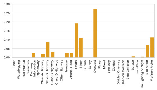
Figure 14.
Average feature importance on the whole dataset.
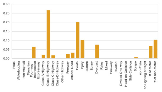
Figure 15.
Average feature importance of the death category.
In addition, we randomly selected 100 incidents, and Figure 16a shows the heatmap of feature importance for these incidents. It can be observed that the important features align with the overall feature ranking in Figure 14, while there are slight differences in feature importance between individual incidents. Figure 16b illustrates the importance of features for “death” incidents, and it also aligns with the feature importance ranking in Figure 15. Therefore, the TabNet model demonstrates good adaptability to various categories, exhibits excellent interpretability for tabular data in traffic incidents, and guides us to focus on relevant features for specific event types.

Figure 16.
Heatmap of the average feature importance; (a) Samples of all incidents; (b) Samples of incidents with death.
5.2. Stepwise Feature Selection
Subsequently, we focused on each step’s feature selection in Figure 17 by exploring the feature mask matrix. N_step was set to be three in this section. It can be observed that step 1 was the most critical, as it encompassed a wide range of features, including “four-way intersection”, “class-A highway”, “freeway”, “injury”, “number of motor vehicles”, and “number of non-motor vehicles”. In step 2, the model paid attention to features such as “death”, “overcast”, and “arterial road”, while in the third step, the focus shifted to “Class-B highway injury” and “overcast”. Similarly, the selected features varied across different individual instances, highlighting the model’s ability to adapt to the specific characteristics of each data point. We interpreted the feature selection in the subsequent steps as a means of addressing any missing features from the previous steps. By iteratively selecting the features at each step, we determined the overall feature selection pattern and the overall feature importance, which were then used for prediction. This improvement over the black-box nature of other deep learning models strikes a balance between training accuracy and interpretability. It allowed us to gain a deeper understanding of the significant factors influencing incident duration and provided us with more informed judgment.

Figure 17.
Heatmap of the sample mask matrix for each step; (a) Step1; (b) Step2; (c) Step3.
6. Conclusions and Future Work
6.1. Conclusions
Traffic incidents often lead to increased congestion, delays, and potential safety hazards for road users. Accurate prediction of the incident duration is crucial to mitigating these consequences by enabling effective resource allocation, improved incident response planning, and efficient traffic management strategies. This study seeks to address several research gaps in the prediction of traffic incident duration. It utilized a comprehensive dataset spanning six years and covering the entire city of Tianjin, China, enabling a thorough analysis of incident types and diverse regions. By adopting the TabNet model, the research achieved a balance between interpretability and predictive accuracy, facilitating the examination of influential factors. The findings provide valuable insights for intelligent traffic management, supporting optimized resource allocation and efficient incident management. Overall, this research contributes to improving traffic flow and system effectiveness.
More specifically, this study preprocessed the incident dataset, utilized the TabNet model, and explored its interpretability to enhance our understanding of the key factors and prediction steps. The TabNet model demonstrates a strong predictive performance, achieving an MAE of 17.04 min, RMSE of 22.01 min, and MAPE of 33.60% on the test dataset, which outperformed most other reference models. Moreover, through the interpretability of the TabNet model, the paper identified and numerically ranked the influential factors affecting the incident duration.
The results also highlighted the road type, casualties, weather conditions (especially overcast), and number of motor and non-motor vehicles as the most significant factors. Hence, some specific road types (e.g., Class-B highways) and regions require the proactive allocation of police resource to effectively manage accident-prone areas. For incidents involving significant casualties, extreme weather conditions, or a large number of vehicles, traffic management authorities should develop pre-planned strategies to minimize incident duration and mitigate the impact on traffic flow. This proactive approach can lead to a timely response, efficient incident clearance, and reduced disruptions to the overall traffic system.
Overall, the TabNet model showcases its effectiveness in predicting traffic incident duration, while offering interpretability to uncover the key factors and prediction steps. By combining the interpretability of tree-based models and the high prediction accuracy of deep neural networks, this study contributes to the field of traffic incident prediction and offers valuable insights for improving traffic management strategies, ultimately enhancing the efficiency and safety of road networks.
6.2. Future Work
Based on the findings of this study, there are several directions for future improvements. Firstly, it is important to note that the incident duration considered in this research focused primarily on the duration of the incident itself, without considering the subsequent recovery of traffic flow to normal conditions. Future studies could investigate and model the process of traffic flow restoration after incidents, which would provide a more comprehensive understanding of the overall impact of incidents on traffic. Secondly, while the TabNet model demonstrated good predictive performance, the complex architecture of TabNet can be computationally expensive. Therefore, we need to continue exploring methods that allow for cost-effective prediction on large-scale and very high-dimensional datasets.
Furthermore, despite its ability to provide feature importance, the interpretability of TabNet is not as straightforward as simpler models such as decision trees or linear regression. Thus, more advanced techniques can be employed to gain deeper insights into the decision-making process of the TabNet model. For instance, techniques such as SHAP (SHapley Additive exPlanations) values or LIME (Local Interpretable Model-agnostic Explanations) could be applied to provide more detailed explanations of the model’s predictions and enhance its interpretability. By addressing these areas, we can further improve the accuracy, interpretability, and comprehensiveness of predicting traffic incident duration, thereby facilitating more effective traffic management.
Author Contributions
Conceptualization, H.L.; methodology, H.L. and Y.L.; software, H.L.; validation, H.L. and Y.L.; formal analysis, H.L.; investigation, H.L. and Y.L.; resources, Y.L.; data curation, H.L.; writing—original draft preparation, H.L.; writing—review and editing, Y.L. All authors have read and agreed to the published version of the manuscript.
Funding
This research was funded by Shanxi Provincial Innovation Center Project for Digital Road Design Technology (202104010911019).
Data Availability Statement
Not applicable.
Conflicts of Interest
The authors declare no conflict of interest.
References
- Mannering, F.L.; Bhat, C.R. Analytic methods in accident research: Methodological frontier and future directions. Anal. Methods Accid. Res. 2014, 1, 1–22. [Google Scholar] [CrossRef]
- Chung, Y.; Chiou, Y.; Lin, C. Simultaneous equation modeling of freeway accident duration and lanes blocked. Anal. Methods Accid. Res. 2015, 7, 16–28. [Google Scholar] [CrossRef]
- Shang, Q.; Xie, T.; Yu, Y. Prediction of duration of traffic incidents by hybrid deep learning based on multi-source incomplete data. Int. J. Environ. Res. Public Health 2022, 19, 10903. [Google Scholar] [CrossRef] [PubMed]
- Tang, J.; Zheng, L.; Han, C.; Yin, W.; Zhang, Y.; Zou, Y.; Huang, H. Statistical and machine-learning methods for clearance time prediction of road incidents: A methodology review. Anal. Methods Accid. Res. 2020, 27, 100123. [Google Scholar] [CrossRef]
- Hamad, K.; Obaid, L.; Nassif, A.B.; Abu Dabous, S.; Al-Ruzouq, R.; Zeiada, W. Comprehensive evaluation of multiple machine learning classifiers for predicting freeway incident duration. Innov. Infrastruct. Solut. 2023, 8, 177. [Google Scholar] [CrossRef]
- Valenti, G.; Lelli, M.; Cucina, D. A comparative study of models for the incident duration prediction. Eur. Transp. Res. Rev. 2010, 2, 103–111. [Google Scholar] [CrossRef]
- Ke, A.; Gao, Z.; Yu, R.; Wang, M.; Wang, X. A hybrid approach for urban expressway traffic incident duration prediction with Cox regression and random survival forests models. In Proceedings of the 2017 IEEE/ACIS 16th International Conference on Computer and Information Science (ICIS), Wuhan, China, 24–26 May 2017; pp. 113–118. [Google Scholar]
- Wang, S.; Li, R.; Guo, M. Application of nonparametric regression in predicting traffic incident duration. Transport 2018, 33, 22–31. [Google Scholar] [CrossRef]
- Chand, S.; Li, Z.; Alsultan, A.; Dixit, V.V. Comparing and Contrasting the Impacts of Macro-Level Factors on Crash Duration and Frequency. Int. J. Environ. Res. Public Health 2022, 19, 5726. [Google Scholar] [CrossRef]
- Yang, L. Clearance time prediction of traffic accidents: A case study in Shandong, China. Australas. J. Disaster Trauma Stud. 2022, 26, 185–194. [Google Scholar]
- Khattak, A.J.; Liu, J.; Wali, B.; Li, X.; Ng, M. Modeling traffic incident duration using quantile regression. Transp. Res. Rec. 2016, 2554, 139–148. [Google Scholar] [CrossRef]
- Li, R.; Pereira, F.C.; Ben-Akiva, M.E. Competing risks mixture model for traffic incident duration prediction. Accid. Anal. Prev. 2015, 75, 192–201. [Google Scholar] [CrossRef] [PubMed]
- Anastasopoulos, P.C.; Labi, S.; Bhargava, A.; Mannering, F.L. Empirical assessment of the likelihood and duration of highway project time delays. J. Constr. Eng. Manag. 2012, 138, 390–398. [Google Scholar] [CrossRef]
- Lin, L.; Wang, Q.; Sadek, A.W. A combined M5P tree and hazard-based duration model for predicting urban freeway traffic accident durations. Accid. Anal. Prev. 2016, 91, 114–126. [Google Scholar] [CrossRef]
- Araghi, B.N.; Hu, S.; Krishnan, R.; Bell, M.; Ochieng, W. A comparative study of k-NN and hazard-based models for incident duration prediction. In Proceedings of the 17th International IEEE Conference on Intelligent Transportation Systems (ITSC), Qingdao, China, 8–11 October 2014; pp. 1608–1613. [Google Scholar]
- Pan, D.; Hamdar, S. From Traffic Analysis to Real-Time Management: A Hazard-Based Modeling for Incident Durations Extracted Through Traffic Detector Data Anomaly Detection. Transp. Res. Rec. 2023, 365415635. [Google Scholar] [CrossRef]
- Hojati, A.T.; Ferreira, L.; Washington, S.; Charles, P. Hazard based models for freeway traffic incident duration. Accid. Anal. Prev. 2013, 52, 171–181. [Google Scholar] [CrossRef]
- Mouhous, F.; Aissani, D.; Farhi, N. A stochastic risk model for incident occurrences and duration in road networks. Transp. A Transp. Sci. 2022, 1–33. [Google Scholar] [CrossRef]
- Zou, Y.; Ye, X.; Henrickson, K.; Tang, J.; Wang, Y. Jointly analyzing freeway traffic incident clearance and response time using a copula-based approach. Transp. Res. Part C Emerg. Technol. 2018, 86, 171–182. [Google Scholar] [CrossRef]
- Zou, Y.; Zhang, Y.; Lord, D. Analyzing different functional forms of the varying weight parameter for finite mixture of negative binomial regression models. Anal. Methods Accid. Res. 2014, 1, 39–52. [Google Scholar] [CrossRef]
- Zou, Y.; Henrickson, K.; Lord, D.; Wang, Y.; Xu, K. Application of finite mixture models for analysing freeway incident clearance time. Transp. A Transp. Sci. 2016, 12, 99–115. [Google Scholar] [CrossRef]
- Zou, Y.; Tang, J.; Wu, L.; Henrickson, K.; Wang, Y. Quantile analysis of factors influencing the time taken to clear road traffic incidents. In Proceedings of the Institution of Civil Engineers-Transport; Thomas Telford Ltd.: London, UK, 2017; Volume 170, pp. 296–304. [Google Scholar]
- Fitzenberger, B.; Wilke, R.A. Using quantile regression for duration analysis. Allg. Stat. Arch. 2006, 90, 105–120. [Google Scholar]
- Wu, W.; Chen, S.; Zheng, C. Traffic incident duration prediction based on support vector regression. In Proceedings of the ICCTP 2011: Towards Sustainable Transportation Systems, Nanjing, China, 17–17 September 2011; American Society of Civil Engineers: Reston, VA, USA, 2011; pp. 2412–2421. [Google Scholar]
- Wang, W.; Chen, H.; Bell, M.C. Vehicle breakdown duration modelling. J. Transp. Stat. 2005, 8, 75–84. [Google Scholar]
- Kim, W.; Chang, G. Development of a hybrid prediction model for freeway incident duration: A case study in Maryland. Int. J. Intell. Transp. Syst. Res. 2012, 10, 22–33. [Google Scholar] [CrossRef]
- Shang, Q.; Tan, D.; Gao, S.; Feng, L. A Hybrid Method for Traffic Incident Duration Prediction Using BOA-Optimized Random Forest Combined with Neighborhood Components Analysis. J. Adv. Transp. 2019, 2019, 4202735. [Google Scholar] [CrossRef]
- Zhao, H.; Gunardi, W.; Liu, Y.; Kiew, C.; Teng, T.; Yang, X.B. Prediction of traffic incident duration using clustering-based ensemble learning method. J. Transp. Eng. Part A Syst. 2022, 148, 4022044. [Google Scholar] [CrossRef]
- Song, Y.; Ying, L.U. Decision tree methods: Applications for classification and prediction. Shanghai Arch. Psychiatry 2015, 27, 130. [Google Scholar] [PubMed]
- Grigorev, A.; Mihaita, A.; Lee, S.; Chen, F. Incident duration prediction using a bi-level machine learning framework with outlier removal and intra–extra joint optimisation. Transp. Res. Part C Emerg. Technol. 2022, 141, 103721. [Google Scholar] [CrossRef]
- Ghosh, B.; Dauwels, J. Comparison of different Bayesian methods for estimating error bars with incident duration prediction. J. Intell. Transp. Syst. 2022, 26, 420–431. [Google Scholar] [CrossRef]
- Park, H.; Haghani, A.; Zhang, X. Interpretation of Bayesian neural networks for predicting the duration of detected incidents. J. Intell. Transp. Syst. 2016, 20, 385–400. [Google Scholar] [CrossRef]
- Boyles, S.; Fajardo, D.; Waller, S.T. A naive Bayesian classifier for incident duration prediction. In Proceedings of the 86th Annual Meeting of the Transportation Research Board, Washington, DC, USA, 1 January 2007. [Google Scholar]
- Zhao, Y.; Deng, W. Prediction in traffic accident duration based on heterogeneous ensemble learning. Appl. Artif. Intell. 2022, 36, 2018643. [Google Scholar] [CrossRef]
- Arik, S.Ö.; Pfister, T. Tabnet: Attentive interpretable tabular learning. In Proceedings of the AAAI Conference on Artificial Intelligence, Virtual Event, 2–9 February 2021; pp. 6679–6687. [Google Scholar]
- Yan, J.; Xu, T.; Yu, Y.; Xu, H. Rainfall forecast model based on the tabnet model. Water 2021, 13, 1272. [Google Scholar] [CrossRef]
- Sun, C.; Li, S.; Cao, D.; Wang, F.; Khajepour, A. Tabular Learning-Based Traffic Event Prediction for Intelligent Social Transportation System. IEEE Trans. Comput. Soc. Syst. 2022, 10, 1199–1210. [Google Scholar] [CrossRef]
- Da Silva, I.N.; Spatti, D.H.; Flauzino, R.A.; Liboni, L.H.B.; Dos Reis Alves, S.F. Artificial Neural Networks; Springer: Cham, Switzerland, 2017. [Google Scholar]
- Hamadneh, N.N.; Tahir, M.; Khan, W.A. Using artificial neural network with prey predator algorithm for prediction of the COVID-19: The case of Brazil and Mexico. Mathematics 2021, 9, 180. [Google Scholar] [CrossRef]
- Kesavaraj, G.; Sukumaran, S. A study on classification techniques in data mining. In Proceedings of the 2013 Fourth International Conference on Computing, Communications and Networking Technologies (ICCCNT), Tiruchengode, India, 4–6 July 2013; pp. 1–7. [Google Scholar]
- Iranitalab, A.; Khattak, A. Comparison of four statistical and machine learning methods for crash severity prediction. Accid. Anal. Prev. 2017, 108, 27–36. [Google Scholar] [CrossRef] [PubMed]
Disclaimer/Publisher’s Note: The statements, opinions and data contained in all publications are solely those of the individual author(s) and contributor(s) and not of MDPI and/or the editor(s). MDPI and/or the editor(s) disclaim responsibility for any injury to people or property resulting from any ideas, methods, instructions or products referred to in the content. |
© 2023 by the authors. Licensee MDPI, Basel, Switzerland. This article is an open access article distributed under the terms and conditions of the Creative Commons Attribution (CC BY) license (https://creativecommons.org/licenses/by/4.0/).