The Impact of Fear on a Harvested Prey–Predator System with Disease in a Prey

Abstract

A mathematical eco-epidemiological model consisting of harvested prey–predator system involving fear and disease in the prey population is formulated and studied. The prey population is supposed to be separated into two groups: susceptible and infected. The susceptible prey grows logistically, whereas the infected prey cannot reproduce and instead competes for the environment’s carrying capacity. Furthermore, the disease is transferred through contact from infected to susceptible individuals, and there is no inherited transmission. The existence, positivity, and boundedness of the model’s solution are discussed. The local stability analysis is carried out. The persistence requirements are established. The global behavior of the system is investigated with the use of the Lyapunov method. An application to the Sotomoyar theorem of local bifurcation is performed around the equilibrium points. In the end, the system is numerically simulated to confirm our obtained analytical results and specify the control set of parameters. Bifurcation diagrams are used to show the dynamical behavior as a function of some parameters. It is obtained that the prey’s fear stabilizes the system, while the disease and harvest cause extinction in one or more species.

1. Introduction

Due to its widespread existence and significance, the dynamic interaction between prey and predator has been the subject of research and will continue to be a crucial topic; see [1,2,3,4,5,6,7,8,9] and the references cited therein. The well-known Lotka–Volterra type prey–predator system has been the focus of numerous good articles since being raised by Lotka and Volterra [10,11]. A Canadian scientist by the name of Holling [12] introduced the comparable functional response functions for diverse species in 1959, including type I, type II, and type III, based on his experimental results, which comprised three fundamental types of predation rates. Since weak (or slow) prey is relevant to Holling type I functional response function, the rate of prey consumption rises linearly. In contrast, type II functional response shows that a predator’s rate of prey intake grows as prey density increases but eventually levels off at a particular point, remaining constant regardless of increases in prey density. The type III functional response, on the other hand, is comparable to the type II response in that saturation happens at high prey density levels. However, at low prey density levels, the graph between the number of prey eaten and the size of the prey population is now a strictly increasing function of prey consumed by predators, making it suitable for the prey with a group defense capability.

The consistent environment is unusual in natural existence. Fear, stage structure, delay, harvesting, toxicity, cannibalism, anti-predator capabilities, refuge, infective disease, and other important factors affecting the population all have an impact on the natural environment. The principal biotic threats to the prey–predator relationship are infectious disease, which causes both species to suffer and has economic consequences, harvesting, and fear, which lowers prey growth. As a result, knowing the impact of biotic and abiotic forces on the ecosystem is critical. Consequently, it is worth looking into the prey–predator system in the context of fear, harvesting, and illness. For many years, mathematical biologists have attempted to integrate the two primary research areas, ecology and epidemiology. Eco-epidemiological refers to the integration of infection into the ecological model [13]. Eco-epidemiological models, which are described as mathematical representations of ecological systems where the disease impacts prey and/or predators, have been the subject of many investigations. When analyzing the effects of disease on an environment, disease in the predator, disease in the prey, and disease in both groups can all be taken into consideration. Predators may eat susceptible and ill animals if the disease is present in the prey. Studies on disease, infection, prey–predator dynamics, and possible ecological and biological implications are mentioned in [14,15,16,17,18,19,20,21,22,23,24]. On the other hand, the impact of harvesting a natural population is one of the most important issues in population ecology. According to Ganguli and Kar [25] and the references therein, harvesting can signify a population decline because of hunting or capturing individuals and removing them from the population. Numerous studies have looked at the dynamic behaviors of harvesting populations because there is so much interest in using bio-economic models; see, for example, [19,21,25,26,27]. This component is also useful for population control [28]. Most of the time, achieving a sizable harvest gain from the population is the aim in addition to population management.

Additionally, fear has a remarkable impact on ecosystems. The impact of terror on prey species was a topic of study for many scholars. The effects of fear can be either direct or indirect; in the former, the predator directly kills the prey [29]. In contrast, in the indirect example, a predator’s presence drastically alters the prey’s behavior due to their dread of the threat of predation [30]. As a result, numerous studies have been conducted to comprehend how prey fear affects the dynamics of the prey–predator system, see [9,31,32,33,34,35,36,37,38,39] and the references therein. Despite the aforementioned, this paper combines the effects of fear, disease, and harvest in a single prey–predator system. Moreover, this paper is structured as follows: In Section 2, we develop a harvested prey–predator model with fear and sickness in prey species and then investigate the existence, boundedness, and non-negativity of solutions. In Section 3, we addressed the equilibria’s stability and persistence. Section 4 focuses on global dynamics. Section 5 investigates the local bifurcation. Section 6 has some numerical simulations, while Section 5 contains concluding observations.

2. Model Construction

In this section, a real-world eco-epidemiological problem is simulated mathematically depending on the following assumptions. First, let $X\left(t\right)$ and $Y\left(t\right)$ be the density of the prey and predator species at time t, respectively. Consider now the assumptions:

• The prey species $X\left(t\right)$ is divided into two compartments due to the existence of the disease in their population: Susceptible prey is denoted by $S\left(t\right)$ and Infected prey is represented by $I\left(t\right)$.
• In the absence of predation, the susceptible prey grows logistically, while the infected prey cannot reproduce; rather, it competes for the carrying capacity of the environment. According to the mass action principle, the disease is transmitted from the infected to susceptible individuals by contact. Finally, the existence of disease causes a specific death rate in the infected population.
• The susceptible prey growth reduces due to the influence of the fear of the predation process by the predator.
• The predator species does not distinguish between the susceptible and infected prey and attack the available prey according to the Holling type-II and Lotka–Volttera functional responses for the susceptible and infected prey, respectively.
• There is an external force that imposes harvesting on the system.

Now, according to the above assumptions, the eco-epidemiological model can be represented as follows:

$$\begin{array}{c}\frac{dS}{dt}=r\left(\theta +\frac{\mu \left(1-\theta \right)}{\mu +Y}\right)S-\alpha S\left(S+I\right)-\beta SI-\frac{a_{1}SY}{b+S}-h_{1}S,\\ \frac{dI}{dt}=\beta SI-a_{2}IY-\left(d_1+h_2\right)I,\\ \frac{dY}{dt}=\frac{e_1{a}_{1}SY}{b+S}+e_2{a}_{2}IY-\left(d_2+h_3\right)Y,\end{array}$$

(1)

with initial condition $S\left(0\right)>0,I\left(0\right)>0,Y\left(0\right)>0$. While the parameters are positive constants and are described the Table 1.

Table 1. The model terms and parameters description.

Parameter or Term	Description
$r$	The susceptible prey’s intrinsic growth rate.
$\theta +\frac{\mu \left(1-\theta \right)}{\mu +Y}\in \left[0,1\right]$	The fear function, where $\mu >0$ is the level of fear and $\theta \in \left[0,1\right]$ is the minimum cost of fear [36].
$\alpha$	The intraspecific competition rate among the prey individuals.
$\beta$	The infection rate.
$a_1$	The maximum attack rate of the predator to the susceptible prey.
$b$	The half saturation constant of the predator.
$a_2$	The maximum attack rate of the predator to the infected prey.
$d_i;i=1,2$	The death rates of the infected prey and a predator, respectively.
$e_i\in \left[0,1\right];i=1,2$	The conversion rates of the susceptible and infected biomass to predator biomass.
$h_i;i=1,2,3$	The harvested rates for the susceptible prey, infected prey, and predator.

Moreover, the solution of system (1) is bounded, as seen in the next theorem. It is easy to confirm that the necessary requirement for the survival of all species in the system (1) is given by:

$$h_1<r$$

(2)

Theorem 1. 

The solutions of system (1) starting in ${ℝ}_{+}^3$ remain positive for all time.

Proof. 

The solution $\left(S\left(t\right),I\left(t\right),Y\left(t\right)\right)$ of the system (1) exists and is unique on $\left[0,\tau \right]$, where $0<\tau <+\infty$ [40], since the right-hand side of the system (1) is continuous and locally Lipschitzian on $C$ (space of continuous functions). Now, from the first equation of Equation (1), it is obtained that

$$S\left(t\right)=S\left(0\right)\exp \left[{{\displaystyle \int }}_0^t\left\{r\left(\theta +\frac{\mu \left(1-\theta \right)}{\mu +Y\left(u\right)}\right)-\alpha \left(S\left(u\right)+I\left(u\right)\right)-\beta I\left(u\right)-\frac{a_{1}Y\left(u\right)}{b+S\left(u\right)}-h_1\right\}du\right]>0.$$

Similarly,

$$I\left(t\right)=I\left(0\right)\exp \left[{{\displaystyle \int }}_0^t\left\{\beta S\left(u\right)-a_{2}Y\left(u\right)-\left(d_1+h_2\right)\right\}du\right]>0,$$

and

$$Y\left(t\right)=Y\left(0\right)\exp \left[{{\displaystyle \int }}_0^t\left\{\frac{e_1{a}_{1}S\left(u\right)}{b+S\left(u\right)}+e_2{a}_{2}I\left(u\right)-\left(d_2+h_3\right)\right\}du\right]>0.$$

Hence, for all starting points in ${ℝ}_{+}^3$, the solution remains positive for all time. □

Theorem 2. 

All solutions of system (1) are uniformly bounded.

Proof: 

From the first equation, it is obtained that

$$\frac{dS}{dt}+\alpha S^2\le \left(r-h_1\right)S$$

Hence,

$$\underset{t\to \infty }{\lim }\sup S\left(t\right)\le \frac{r-h_1}{\alpha }.$$

Let $M\left(t\right)=S\left(t\right)+I\left(t\right)+Y\left(t\right)$, then applying some calculations gives that

$$\begin{array}{c}\frac{dM}{dt}\le \left(r-h_1\right)S-\left(d_1+h_2\right)I-\left(d_2+h_3\right)Y\\ =\left(r-h_1+1\right)S-S-\left(d_1+h_2\right)I-\left(d_2+h_3\right)Y\\ \le \left(r-h_1+1\right)\frac{r-h_1}{\alpha }-LM=N-LM\end{array}$$

where $L=min\left\{1,d_1+h_2,d_2+h_3\right\}$, and $N=\frac{{\left(r-h_1\right)}^2}{\alpha }+\frac{r-h_1}{\alpha }$. Direct computation gives that

$$M\left(t\right)\le \frac{N}{L}\left(1-e^{-Lt}\right)+M\left(0\right)e^{-Lt}$$

Therefore, for $t\to \infty$, it is obtained that $M\left(t\right)\le \frac{N}{L}$. Therefore, all of the system (1)’s solutions will reach the region:

$$D=\left\{\left(S,I,Y\right)\in {ℝ}_{+}^3:S\left(t\right)\le \frac{r-h_1}{\alpha },0<M\left(t\right)\le \frac{N}{L}\right\}$$

Thus, all the solutions are uniformly bounded. □

3. Stability Analysis with Persistence

In this part, the existence of the equilibrium points $\left(E.P\right),$ stability analysis, and persistence of the system (1) are studied. It is spotted that the next equilibrium points exist as follows:

The vanishing equilibrium point $\left(V.E.P\right)$, which is denoted by $m_0=\left(0,0,0\right)$ always exists.

The axial equilibrium point $\left(A.E.P\right)$ is denoted by $m_1=\left(\widehat{S},0,0\right)$ where $\widehat{S}=\frac{r-h_1}{\alpha }$, exists under Condition (2).

The predator-free equilibrium point $\left(P.F.E.P\right)$ that is denoted by $m_2=\left(\overline{S},\overline{I},0\right)$, where

$$\overline{S}=\frac{d_1+h_2}{\beta },\overline{I}=\frac{\left(r-h_1\right)\beta -\alpha (d_1+h_2)}{\beta \left(\alpha +\beta \right)},$$

(3)

exists if the following condition holds:

$$\alpha (d_1+h_2)<\left(r-h_1\right)\beta$$

(4)

The disease-free equilibrium point $\left(D.F.E.P\right)$ that is denoted by $m_3=\left(\tilde{S},0,\tilde{Y}\right)$, where

$$\tilde{S}=\frac{b\left(d_2+h_3\right)}{e_1{a}_1-\left(d_2+h_3\right)},$$

(5)

while $\tilde{Y}$ is a positive root of the following second-order polynomial equation

$$B_1{Y}^2+B_{2}Y+B_3=0,$$

(6)

where

$$\begin{array}{l}{B}_1=-{\left[a_1{e}_1-d_2-h_3\right]}^2,\\ B_2=-\mu {\left[d_2+h_3-a_1{e}_1\right]}^2-b^2\alpha e_1\left(d_2+h_3\right)-b{e}_1\left(r\theta -h_1\right)\left[d_2+h_3-a_1{e}_1\right].\\ B_3=-b\mu e_1\left[b\alpha \left(d_2+h_3\right)-\left(r-h_1\right)\left(a_1{e}_1-d_2-h_3\right)\right].\end{array}$$

Obviously, $m_3$ exists uniquely in the positive quadrant of the $SY$-plane provided that the following requirements are met.

$$\left(d_2+h_3\right)<e_1{a}_1.$$

(7)

$$b\alpha \left(d_2+h_3\right)<\left(r-h_1\right)\left(a_1{e}_1-d_2-h_3\right).$$

(8)

The positive equilibrium point $\left(P.E.P\right)$ that is denoted by $m_4=\left(S^{\ast },I^{\ast },Y^{\ast }\right)$, where

$$\begin{array}{c}{I}^{\ast }=\frac{\left(b+S^{\ast }\right)\left(d_2+h_3\right)-S^{\ast }{a}_1{e}_1}{\left(b+S^{\ast }\right)a_2{e}_2}\\ Y^{\ast }=\frac{S^{\ast }\beta -\left(d_1+h_2\right)}{a_2}\end{array}\}.$$

(9)

While $S^{\ast }$ is a positive root of the following third-order polynomial equation

$$E_1{S}^3+E_2{S}^2+E_{3}S+E_4=0,$$

(10)

where

$$\begin{array}{l}{E}_1=\alpha \beta a_2{e}_2.\\ \begin{array}{c}{E}_2=\beta \left(\alpha +\beta \right)\left(d_2-a_1{e}_1+h_3\right)+e_2[{\beta }^2{a}_1+\beta a_2\left(b\alpha -r\theta +h_1\right)\\ +\alpha a_2\left(\mu a_2-d_1-1\right)]\end{array}.\\ \begin{array}{c}{E}_3=\left(\alpha +\beta \right)\left[\left(d_2+h_3\right)\left(b\beta +\mu a_2\right)-\mu a_1{a}_2{e}_1+\left(d_1+h_2\right)\left(a_1{e}_1-d_2-h_3\right)\right]\\ -e_2\left(d_1+h_2\right)\left[2\beta a_1+a_2\left(b\alpha -r\theta +h_1\right)\right]\\ +a_2{e}_2{h}_1\left(b\beta +\mu a_2\right)+\beta a_2{e}_2\left(\mu a_1-br\theta \right)+\mu a_2^2{e}_2\left(b\alpha -r\right)\end{array}.\\ \begin{array}{c}{E}_4=\left(\alpha +\beta \right)\left(d_2+h_3\right)\left[b\mu a_2-b\left(d_1+h_2\right)\right]-a_2{e}_2\left[br\mu a_2+\left(\mu a_1-br\theta \right)d_1\right]\\ +a_1{e}_2{\left(d_1+h_2\right)}^2+b{a}_2{e}_2{h}_1\left(\mu a_2-d_1\right)+a_2{e}_2{h}_2\left(br\theta -\mu a_1-b{h}_1\right)\end{array}.\end{array}$$

So by Descartes’ rule of sign, Equation (10) has a unique positive root, and hence, P.E.P exists uniquely in the interior of ${ℝ}_{+}^3$ provided that the following condition is met

$$\frac{\left(d_1+h_2\right)}{\beta }<S^{\ast }<\frac{\left(b+S^{\ast }\right)\left(d_2+h_3\right)}{a_1{e}_1},$$

(11)

with one set of the following sets of conditions.

$$\begin{array}{c}{E}_2>0,E_3\ne 0,E_4<0\\ E_2\ne 0,E_3<0,E_4<0\end{array}\}.$$

(12)

Now, the local stability of the above equilibrium points of system (1) is studied. The Jacobian matrix at $m_0=\left(0,0,0\right)$ can be written as

$$J\left(m_0\right)=\left[\begin{array}{ccc}r-h_1& 0& 0\\ 0& -\left(d_1+h_2\right)& 0\\ 0& 0& -\left(d_2+h_3\right)\end{array}\right].$$

(13)

Obviously, the eigenvalues of $J\left(m_0\right)$ are given by:

$${\lambda }_{01}=r-h_1,{\lambda }_{02}=-\left(d_1+h_2\right)<0,{\lambda }_{03}=-\left(d_2+h_3\right)<0.$$

(14)

Hence, the V.E.P is locally asymptotically stable (L.A.S) if and only if the survival Condition (2) is reflected $\left(r<h_1\right)$, and otherwise, it is a saddle point.

The Jacobian matrix at $m_1=\left(\frac{r-h_1}{\alpha },0,0\right)$ can be written as

$$J\left(m_1\right)=\left[\begin{array}{ccc}-r+h_1& -\frac{\left(\alpha +\beta \right)\left(r-h_1\right)}{\alpha }& -\frac{\left(r\left(1-\theta \right)\left(b\alpha +r-h_1\right)+a_1\alpha \mu \right)\left(r-h_1\right)}{\mu \alpha \left(b\alpha +r-h_1\right)}\\ 0& \frac{\beta \left(r-h_1\right)-\alpha \left(d_1+h_2\right)}{\alpha }& 0\\ 0& 0& \frac{a_1{e}_1\left(r-h_1\right)}{\left(b\alpha +r-h_1\right)}-\left(d_2+h_3\right)\end{array}\right].$$

(15)

So, the eigenvalues of $J\left(m_1\right)$ are given by

$${\lambda }_{11}=-\left(r-h_1\right)<0,{\lambda }_{12}=\frac{\beta \left(r-h_1\right)-\alpha \left(d_1+h_2\right)}{\alpha },{\lambda }_{13}=\frac{a_1{e}_1\left(r-h_1\right)}{\left(b\alpha +r-h_1\right)}-\left(d_2+h_3\right).$$

(16)

Therefore, the A.E.P. is a L.A.S provided that the following condition holds:

$$\begin{array}{c}\beta \left(r-h_1\right)<\alpha \left(d_1+h_2\right)\\ \frac{a_1{e}_1\left(r-h_1\right)}{\left(b\alpha +r-h_1\right)}<\left(d_2+h_3\right)\end{array}\}.$$

(17)

The Jacobian matrix at $m_2=\left(\overline{S},\overline{I},0\right)$ can be written as

$$J\left(m_2\right)=\left[\begin{array}{ccc}-\alpha \overline{S}& -\left(\alpha +\beta \right)\overline{S}& -\left(\frac{r\left(1-\theta \right)}{\mu }+\frac{a_1}{b+\overline{S}}\right)\overline{S}\\ \beta \overline{I}& 0& -a_2\overline{I}\\ 0& 0& \frac{e_1{a}_1\overline{S}}{b+\overline{S}}+e_2{a}_2\overline{I}-\left(d_2+h_3\right)\end{array}\right].$$

(18)

The characteristic equation of $J\left(m_2\right)$ can be determined as follows:

$$\left({\lambda }^2-T_2\lambda +D_2\right)\left(\frac{e_1{a}_1\overline{S}}{b+\overline{S}}+e_2{a}_2\overline{I}-\left(d_2+h_3\right)-\lambda \right)=0,$$

(19)

where $T_2=-\alpha \overline{S}<0$, and $D_2=\beta \left(\alpha +\beta \right)\overline{S}\overline{I}>0$.

Since, $T_2<0$ and $D_2>0$, then the two eigenvalues obtain from the first factor of Equation (19) have negative real parts. While the third eigenvalue is given by ${\lambda }_{23}=\frac{e_1{a}_1\overline{S}}{b+\overline{S}}+e_2{a}_2\overline{I}-\left(d_2+h_3\right)$, will be negative, provided that the following condition holds.

$$\frac{e_1{a}_1\overline{S}}{b+\overline{S}}+e_2{a}_2\overline{I}<\left(d_2+h_3\right).$$

(20)

Accordingly, the P.F.E.P. is a L.A.S. provided that Condition (20) is met.

The Jacobian matrix at $m_3=\left(\tilde{S},0,\tilde{Y}\right)$ can be written as

$$J\left(m_3\right)=\left[\begin{array}{ccc}-\alpha \tilde{S}+\frac{a_1\tilde{Y}}{{\left(b+\tilde{S}\right)}^2}& -\left(\alpha +\beta \right)\tilde{S}& -\left(\frac{r\mu \left(1-\theta \right)}{{\left(\mu +\tilde{Y}\right)}^2}+\frac{a_1}{b+\tilde{S}}\right)\tilde{S}\\ 0& \beta \tilde{S}-a_2\tilde{Y}-\left(d_1+h_2\right)& 0\\ \frac{b{e}_1{a}_1}{{\left(b+\tilde{S}\right)}^2}\tilde{Y}& e_2{a}_2\tilde{Y}& 0\end{array}\right].$$

(21)

The characteristic equation of $J\left(m_3\right)$ can be determined as follows:

$$\left({\lambda }^2-T_3\lambda +D_3\right)\left(\beta \tilde{S}-a_2\tilde{Y}-\left(d_1+h_2\right)-\lambda \right)=0,$$

(22)

where $T_3=-\alpha \tilde{S}+\frac{a_1\tilde{Y}}{{\left(b+\tilde{S}\right)}^2}$, and $D_3=\frac{b{e}_1{a}_1}{{\left(b+\tilde{S}\right)}^2}\left(\frac{r\mu \left(1-\theta \right)}{{\left(\mu +\tilde{Y}\right)}^2}+\frac{a_1}{b+\tilde{S}}\right)\tilde{S}\tilde{Y}>0$.

It is easy to verify that all the eigenvalues have negative real parts and D.F.E.P. is L.A.S. if the following condition holds.

$$\beta \tilde{S}<a_2\tilde{Y}+\left(d_1+h_2\right).$$

(23)

$$a_1\tilde{Y}<\alpha \tilde{S}{\left(b+\tilde{S}\right)}^2.$$

(24)

Finally, The Jacobian matrix at $m_4=\left(S^{\ast },I^{\ast },Y^{\ast }\right)$ can be written as

$$J\left(m_4\right)=\left[\begin{array}{ccc}-\alpha +\frac{a_1{Y}^{\ast }}{{\left(b+S^{\ast }\right)}^2}& -\left(\alpha +\beta \right)S^{\ast }& -\left(\frac{r\mu \left(1-\theta \right)}{{\left(\mu +Y^{\ast }\right)}^2}+\frac{a_1}{b+S^{\ast }}\right)S^{\ast }\\ \beta I^{\ast }& 0& -a_2{I}^{\ast }\\ \frac{b{e}_1{a}_1{Y}^{\ast }}{{\left(b+S^{\ast }\right)}^2}& e_2{a}_2{Y}^{\ast }& 0\end{array}\right]={\left[a_{ij}\right]}_{3\times 3}.$$

(25)

Then, the characteristic equation of $J\left(m_4\right)$ is

$${\lambda }^3+A_1{\lambda }^2+A_2\lambda +A_3=0,$$

(26)

where

$$\begin{array}{l}{A}_1=-a_{11},\\ A_2=-\left(a_{23}{a}_{32}+a_{12}{a}_{21}+a_{13}{a}_{31}\right),\\ A_3=a_{23}\left(a_{11}{a}_{32}-a_{12}{a}_{31}\right)-a_{21}{a}_{32}{a}_{13},\end{array}$$

While

$$\Delta =A_1{A}_2-A_3=a_{11}{a}_{12}{a}_{21}+a_{13}\left(a_{11}{a}_{31}+a_{21}{a}_{32}\right)+a_{12}{a}_{23}{a}_{31}.$$

Consequently, the L.A.S requirements of P.E.P. can be constructed in the following theorem.

Theorem 3. 

A P.E.P. of the system (1) is L.A.S. if and only if the following condition is met.

$$\max \left\{\frac{a_1{Y}^{\ast }}{{\left(b+S^{\ast }\right)}^2}+\frac{b{e}_1{a}_1\left(\alpha +\beta \right)S^{\ast }}{e_2{a}_2{\left(b+S^{\ast }\right)}^2},\frac{a_1{Y}^{\ast }}{{\left(b+S^{\ast }\right)}^2}+\frac{e_2{a}_2\beta I^{\ast }{\left(b+S^{\ast }\right)}^2}{b{e}_1{a}_1}\right\}<\alpha .$$

(27)

Proof. 

According to the Routh–Hurwitz criterion, the roots of the Jacobian matrix $J\left(m_4\right)$ have negative real parts provided that $A_1>0,A_3>0,\mathrm{and}\Delta >0$. Direct computation shows that Condition (27) guarantees the satisfaction of Routh–Hurwitz criterion requirements. Hence the proof is done.

In the following, the persistence requirements of the system (1) are investigated. It is clear that system (1) has two subsystems lying in the non-negative quadrant of $SI$ and $SY$ planes. These subsystems can be written as

$$\begin{array}{c}S\left[r-\alpha S-\left(\alpha +\beta \right)I-h_1\right]={\varphi }_1\left(S,I\right)\\ I\left[\beta S-\left(d_1+h_2\right)\right]={\varphi }_2\left(S,I\right)\end{array}.$$

(28)

$$\begin{array}{c}S\left[r\left(\theta +\frac{\mu \left(1-\theta \right)}{\mu +Y}\right)-\alpha S-\frac{a_{1}Y}{b+S}-h_1\right]={\rho }_1\left(S,I\right)\\ Y\left[\frac{e_1{a}_{1}S}{b+S}-\left(d_2+h_3\right)\right]={\rho }_2\left(S,I\right)\end{array}.$$

(29)

Clearly, each of these subsystems has three nonnegative equilibrium points that represent the projection of the corresponding boundary equilibrium points of the system (1).

Define the Dulac functions as $B_1\left(S,I\right)=\frac{1}{SI}$ and $B_2\left(S,Y\right)=\frac{1}{SY}$ that are obviously $B_1\left(S,I\right)>0$, $B_2\left(S,Y\right)>0$, and $C^1$ functions in the $Int.{ℝ}_{+}^2$ of the $SI$ and $SY$ planes. Now, direct computation gives that

$$\Delta \left(S,I\right)=\frac{\partial \left(B_1{\varphi }_1\right)}{\partial S}+\frac{\partial \left(B_1{\varphi }_2\right)}{\partial I}=-\frac{\alpha }{I}<0.$$

$$\Delta \left(S,Y\right)=\frac{\partial \left(B_2{\rho }_1\right)}{\partial S}+\frac{\partial \left(B_2{\rho }_{21}\right)}{\partial Y}=-\frac{\alpha }{Y}+\frac{a_1}{{\left(b+S\right)}^2}.$$

Then, the expression $\Delta \left(S,I\right)$ is always negative, and hence, the first subsystem (28) does not contain a periodic dynamic fall in the positive quadrant of the $SI$-plane. However, the expression $\Delta \left(S,Y\right)$ does not identically zero in the $Int.{ℝ}_{+}^2$ of the $SY$-plane and does not change the sign under the condition

$$\frac{a_{1}Y}{{\left(b+S\right)}^2}<\alpha .$$

(30)

Therefore, by using the Dulac–Bendixson criterion [41], there is no closed curve lying in the $Int.{ℝ}_{+}^2$ of the $SY$-plane for all the trajectories satisfying Condition (30). Hence, according to the Poincare–Bendixon theorem [41], the interior equilibrium points of the subsystems (28) and (29) that are given by $m_2$ and $m_3$ respectively, will be a globally asymptotically stable G.A.S whenever they are L.A.S. □

Theorem 4. 

Assume that Condition (30) holds, then system (1) is uniformly persistent if the following conditions are met.

$$\alpha \left(d_1+h_2\right)<\beta \left(r-h_1\right).$$

(31)

$$\left(d_2+h_3\right)<\frac{e_1{a}_1\overline{S}}{b+\overline{S}}+e_2{a}_2\overline{I}.$$

(32)

$$a_2\tilde{Y}+\left(d_1+h_2\right)<\beta \tilde{S}.$$

(33)

Proof. 

Consider the following function: $\left(S,I,Y\right)=S^{p_1}{I}^{p_2}{Y}^{p_3}$, where $p_j$, $\forall j=1,2,3$ are positive constants. Clearly, $\xi \left(S,I,Y\right)>0\mathrm{for}\mathrm{all}\left(S,I,Y\right)\in Int.{ℝ}_{+}^3$ and $\xi \left(S,I,Y\right)\to 0$, when $S\to 0$,$I\to 0$, or $Y\to 0$. Consequently, it is obtained that

$$\begin{array}{c}\mathsf{\Omega }\left(S,I,Y\right)=\frac{{\xi }^{\prime }\left(S,I,Y\right)}{\xi \left(S,I,Y\right)}=p_1\left[r\left(\theta +\frac{\mu \left(1-\theta \right)}{\mu +Y}\right)-\alpha \left(S+I\right)-\beta I-\frac{a_{1}Y}{b+S}-h_1\right]\\ +p_2\left[\beta S-a_{2}Y-\left(d_1+h_2\right)\right]+p_3\left[\frac{e_1{a}_{1}S}{b+S}+e_2{a}_{2}I-\left(d_2+h_3\right)\right]\end{array}.$$

Now the proof follows if $\mathsf{\Omega }\left(P\right)>0$ for any boundary equilibrium point $P$, with a suitable choice of constants $p_1>0$, $p_2>0$, and $p_3>0$.

$$\begin{array}{l}\mathsf{\Omega }\left(m_0\right)=p_1\left(r-h_1\right)-p_2\left(d_1+h_2\right)-p_3\left(d_2+h_3\right).\\ \mathsf{\Omega }\left(m_1\right)=p_2\left(\beta \widehat{S}-\left(d_1+h_2\right)\right)+p_3\left(\frac{e_1{a}_1\widehat{S}}{b+\widehat{S}}-\left(d_2+h_3\right)\right).\\ \mathsf{\Omega }\left(m_2\right)=p_3\left(\frac{e_1{a}_1\overline{S}}{b+\overline{S}}+e_2{a}_2\overline{I}-\left(d_2+h_3\right)\right).\\ \mathsf{\Omega }\left(m_3\right)=p_2\left(\beta \tilde{S}-a_2\tilde{Y}-\left(d_1+h_2\right)\right).\end{array}$$

Clearly, Condition (31) guarantees that $\mathsf{\Omega }\left(m_0\right)>0$, under Condition (31) with a suitable choice of positive constants $p_j$, so that $p_1$ is sufficiently larger than $p_2$ and $p_3$. Moreover, $\mathsf{\Omega }\left(m_1\right)>0$, for a suitable choice of positive constants $p_j$, so that $p_2$ is sufficiently larger than $p_3$. Finally, $\mathsf{\Omega }\left(m_j\right)>0;j=2,3$ due to Conditions (32) and (33), respectively. Thus the proof is performed. □

4. Global Dynamics

In this section, an investigation of the global dynamics of the system (1) around each L.A.S. point is carried out utilizing a suitable Lyapunov function.

Theorem 5. 

The V.E.P. is a G.A.S. whenever it is L.A.S. provided that the following condition holds

$$e_2<e_1.$$

(34)

Proof. 

Define the function $W_0\left(S,I,Y\right)=S+I+\frac{1}{e_1}Y$. Clearly, the function $W_0$ is a positive definite so that $W_0\left(0,0,0\right)=0$ and $W_0\left(S,I,Y\right)>0$ for all $\left(S,I,Y\right)\in {ℝ}_{+}^3$ with $\left(S,I,Y\right)\ne \left(0,0,0\right)$. Then, the derivative $\frac{d{W}_0}{dt}$ can be determined as

$$\frac{d{W}_0}{dt}=r\left(\theta +\frac{\mu \left(1-\theta \right)}{\mu +Y}\right)S-\alpha S\left(S+I\right)-h_{1}S-a_2\left(1-\frac{e_2}{e_1}\right)IY-\left(d_1+h_2\right)I-\frac{\left(d_2+h_3\right)}{e_1}Y.$$

Now, using Condition (34) and after some algebraic manipulation, it is obtained that

$$\frac{d{W}_0}{dt}\le \left(r-h_1\right)S-\left(d_1+h_2\right)I-\frac{\left(d_2+h_3\right)}{e_1}Y.$$

Therefore, $\frac{d{W}_0}{dt}$ is negative definite due to the L.A.S. condition of $m_0$. Hence, the V.E.P. is a G.A.S. point whenever it is L.A.S. under Condition (34). □

Theorem 6. 

The A.E.P. is a G.A.S. whenever it is a L.A.S. provided that the following conditions are met along with the Condition (34).

$$\left(\alpha +\beta \right)\widehat{S}<\left(d_1+h_2\right).$$

(35)

$$\frac{a_1\widehat{S}}{b}+\frac{r\left(1-\theta \right)\widehat{S}}{\mu }<\frac{\left(d_2+h_3\right)}{e_1}.$$

(36)

Proof. 

Define the function $W_1\left(S,I,Y\right)={{\displaystyle \int }}_{\widehat{S}}^S\frac{u-\widehat{S}}{u}du+I+\frac{1}{e_1}Y$. Clearly, the function $W_1$ is positive definite so that $W_1\left(\widehat{S},0,0\right)=0$ and $W_1\left(S,I,Y\right)>0$ for all $\left(S,I,Y\right)\in {ℝ}_{+}^3$ with $\left(S,I,Y\right)\ne \left(\widehat{S},0,0\right)$ and $S>0$. Then, the derivative $\frac{d{W}_1}{dt}$ can be determined as

$$\begin{array}{c}\frac{d{W}_1}{dt}\le -\alpha {\left(S-\widehat{S}\right)}^2-\left[\left(d_1+h_2\right)-\left(\alpha +\beta \right)\widehat{S}\right]I-a_2\left(1-\frac{e_2}{e_1}\right)IY\\ -\left[\frac{\left(d_2+h_3\right)}{e_1}-\frac{a_1\widehat{S}}{b+S}-\frac{r\left(1-\theta \right)\widehat{S}}{\mu +Y}\right]Y\end{array}.$$

Now, using Conditions (34)–(36) and after some algebraic manipulation it is obtained that

$$\frac{d{W}_1}{dt}\le -\alpha {\left(S-\widehat{S}\right)}^2-\left[\left(d_1+h_2\right)-\left(\alpha +\beta \right)\widehat{S}\right]I-\left[\frac{\left(d_2+h_3\right)}{e_1}-\frac{a_1\widehat{S}}{b+S}-\frac{r\left(1-\theta \right)\widehat{S}}{\mu +Y}\right]Y.$$

Therefore, $\frac{d{W}_1}{dt}$ is negative definite due to the given conditions. Hence, the A.E.P. is a G.A.S., and the proof is complete. □

Theorem 7. 

The basin of attraction of the P.F.E.P is given by the region $B\left(m_2\right)=\left\{\left(S,I,Y\right)\in {ℝ}_{+}^3:S>\overline{S},I>\overline{I},Y\ge 0\right\}$ provided that the following condition is met along with Condition (34).

$$\frac{r\left(1-\theta \right)\overline{S}}{\mu }+\frac{a_1\overline{S}}{b}+a_2\overline{I}<\frac{\left(d_2+h_3\right)}{e_1}.$$

(37)

Proof. 

Consider the following function: $W_2\left(S,I,Y\right)={\int }_{\overline{S}}^S\frac{u-\overline{S}}{u}du+{\int }_{\overline{I}}^I\frac{v-\overline{I}}{v}dv+\frac{1}{e_1}Y$. Clearly, the function $W_2\left(S,I,Y\right)>0$ is a continuously differentiable real-valued function for all $\left(S,I,Y\right)\in {ℝ}_{+}^3$ with $\left(S,I,Y\right)\ne \left(\overline{S},\overline{I},0\right)$ and $W_2\left(\overline{S},\overline{I},0\right)=0$. Then, the derivative $\frac{d{W}_2}{dt}$ can be determined as

$$\begin{array}{c}\frac{d{W}_2}{dt}\le -\alpha {\left(S-\overline{S}\right)}^2-\alpha \left(S-\overline{S}\right)\left(I-\overline{I}\right)-a_2\left(1-\frac{e_2}{e_1}\right)IY\\ -\left[\frac{\left(d_2+h_3\right)}{e_1}-\frac{r\left(1-\theta \right)\overline{S}}{\mu +Y}-\frac{a_1\overline{S}}{b+S}-a_2\overline{I}\right]Y\end{array}.$$

So, by using Conditions (34) and (37), it is then obtained after some algebraic manipulation that

$$\frac{d{W}_2}{dt}\le -\alpha {\left(S-\overline{S}\right)}^2-\alpha \left(S-\overline{S}\right)\left(I-\overline{I}\right)-\left[\frac{\left(d_2+h_3\right)}{e_1}-\frac{r\left(1-\theta \right)\overline{S}}{\mu +Y}-\frac{a_1\overline{S}}{b+S}-a_2\overline{I}\right]Y.$$

Therefore, $\frac{d{W}_2}{dt}$ is negative definite due to the given conditions in the region $B\left(m_2\right)$. Hence, the proof is complete. □

Theorem 8. 

The basin of attraction of the D.F.E.P is given by the region $B\left(m_3\right)=\left\{\left(S,I,Y\right)\in {ℝ}_{+}^3:S>\overline{S},I\ge 0,Y>\tilde{Y}\right\}$ provided that the following conditions are met along with Condition (34).

$$\frac{a_1\tilde{Y}}{\left(b+S\right)\left(b+\tilde{S}\right)}<\alpha$$

(38)

$$\left(\alpha +\beta \right)\tilde{S}<\left(d_1+h_2\right)+\frac{e_2{a}_2}{e_1}\tilde{Y}$$

(39)

Proof. 

Consider the following function: $W_3\left(S,I,Y\right)={\int }_{\tilde{S}}^S\frac{u-\tilde{S}}{u}du+I+\frac{1}{e_1}{\int }_{\tilde{Y}}^Y\frac{w-\tilde{Y}}{w}dw$. Clearly, the function $W_3\left(S,I,Y\right)>0$ is a continuously differentiable real-valued function for all $\left(S,I,Y\right)\in {ℝ}_{+}^3$ with $\left(S,I,Y\right)\ne \left(\tilde{S},0,\tilde{Y}\right)$ and $W_3\left(\tilde{S},0,\tilde{Y}\right)=0$. Then, the derivative $\frac{d{W}_3}{dt}$ can be determined as

$$\begin{array}{c}\frac{d{W}_3}{dt}\le -\left[\alpha -\frac{a_1\tilde{Y}}{\left(b+S\right)\left(b+\tilde{S}\right)}\right]{\left(S-\tilde{S}\right)}^2-\left[\frac{\mu r\left(1-\theta \right)}{\left(\mu +Y\right)\left(\mu +\tilde{Y}\right)}+\frac{a_1\tilde{S}}{\left(b+S\right)\left(b+\tilde{S}\right)}\right]\left(S-\tilde{S}\right)\left(Y-\tilde{Y}\right)\\ -a_2\left(1-\frac{e_2}{e_1}\right)IY-\left[\left(d_1+h_2\right)+\frac{e_2{a}_2}{e_1}\tilde{Y}-\left(\alpha +\beta \right)\tilde{S}\right]I\end{array}.$$

So, by using Conditions (34), (38), and (39), it is obtained after some algebraic manipulation that

$$\begin{array}{c}\frac{d{W}_3}{dt}\le -\left[\alpha -\frac{a_1\tilde{Y}}{\left(b+S\right)\left(b+\tilde{S}\right)}\right]{\left(S-\tilde{S}\right)}^2-\left[\frac{\mu r\left(1-\theta \right)}{\left(\mu +Y\right)\left(\mu +\tilde{Y}\right)}+\frac{a_1\tilde{S}}{\left(b+S\right)\left(b+\tilde{S}\right)}\right]\left(S-\tilde{S}\right)\left(Y-\tilde{Y}\right)\\ -\left[\left(d_1+h_2\right)+\frac{e_2{a}_2}{e_1}\tilde{Y}-\left(\alpha +\beta \right)\tilde{S}\right]I\end{array}.$$

Therefore, $\frac{d{W}_3}{dt}$ is negative definite due to the given conditions in the region $B\left(m_3\right)$. Hence, the proof is complete. □

Theorem 9. 

The basin of attraction of the P.E.P is given by the region $B\left(m_4\right)=\left\{\left(S,I,Y\right)\in {ℝ}_{+}^3:S>S^{\ast },I\ge I^{\ast },Y>Y^{\ast }\right\}$ provided that the following conditions are met along with Condition (34). 

$$\frac{a_1{Y}^{\ast }}{\left(b+S\right)\left(b+S^{\ast }\right)}<\alpha .$$

(40)

$$\frac{a_1{S}^{\ast }}{\left(b+S\right)\left(b+S^{\ast }\right)}<\frac{r\mu \left(1-\theta \right)}{\left(\mu +Y\right)\left(\mu +Y^{\ast }\right)}.$$

(41)

Proof. 

Consider the function: $W_4\left(S,I,Y\right)={\int }_{S^{\ast }}^S\frac{u-S^{\ast }}{u}du+{\int }_{I^{\ast }}^I\frac{v-I^{\ast }}{v}dv+\frac{1}{e_1}{\int }_{Y^{\ast }}^Y\frac{w-Y^{\ast }}{w}dw$. Clearly, the function $W_4\left(S,I,Y\right)>0$ is a continuously differentiable real-valued function for all $\left(S,I,Y\right)\in {ℝ}_{+}^3$ with $\left(S,I,Y\right)\ne \left(S^{\ast },I^{\ast },Y^{\ast }\right)$ and $W_4\left(S^{\ast },I^{\ast },Y^{\ast }\right)=0$. Then, the derivative $\frac{d{W}_4}{dt}$ can be determined as

$$\begin{array}{c}\frac{d{W}_4}{dt}=-\left(\alpha -\frac{a_1{Y}^{\ast }}{\left(b+S\right)\left(b+S^{\ast }\right)}\right){\left(S-S^{\ast }\right)}^2-\alpha \left(S-S^{\ast }\right)\left(I-I^{\ast }\right)\\ -\left(\frac{r\mu \left(1-\theta \right)}{\left(\mu +Y\right)\left(\mu +Y^{\ast }\right)}-\frac{a_1{S}^{\ast }}{\left(b+S\right)\left(b+S^{\ast }\right)}\right)\left(S-S^{\ast }\right)\left(Y-Y^{\ast }\right)\\ -a_2\left(1-\frac{e_2}{e_1}\right)\left(I-I^{\ast }\right)\left(Y-Y^{\ast }\right)\end{array}.$$

So, by using Conditions (34), (40) and (41), it is obtained that $\frac{d{W}_4}{dt}$ is negative definite due to the given conditions in the region $B\left(m_4\right)$. Hence, the proof is complete. □

5. Local Bifurcation

By using Sotomayor’s theorem [41], the local bifurcation (L.B.) around the equilibrium points of system (1) is explored. It is common knowledge that a non-hyperbolic equilibrium point is a requirement, but not a sufficient one, for bifurcation to take place. In order to ensure that the equilibrium point is non-hyperbolic at a given value of the parameter, the candidate bifurcation parameter is chosen. Now, rewrite system (1) in the form:

$$\frac{dX}{dt}=F\left(X\right)$$

(42)

where $\mathit{X}={\left(S,I,Y\right)}^{\mathrm{T}}$ and $\mathit{F}={\left(S{f}_1,I{f}_2,Y{f}_3\right)}^{\mathrm{T}}$ with $f_i;i=1,2,3$ represent the interaction functions on the right-hand side of the system (1). Then, using the Jacobian matrix of system (1), simple computation demonstrates that we have the following second directional derivative for every non-zero vector $V={\left(v_1,v_2,v_3\right)}^{\mathrm{T}}$, and $\mathsf{\vartheta }\in {ℝ}_{+}$.

$$D^{2}F\left(X,\mathsf{\vartheta }\right)\left(V,V\right)={\left[k_{i1}\right]}_{3\times 1},$$

(43)

where

$$\begin{array}{l}\begin{array}{c}{k}_{11}=-2\left(\alpha -\frac{a_{1}bY}{{\left(b+S\right)}^3}\right)v_1{}^2-2\left(\frac{r\mu \left(1-\theta \right)}{{\left(\mu +Y\right)}^2}+\frac{a_{1}b}{{\left(b+S\right)}^2}\right)v_1{v}_3\\ -2\left(\alpha +\beta \right)v_1{v}_2+2\left(\frac{r\mu \left(1-\theta \right)S}{{\left(\mu +Y\right)}^3}\right)v_3{}^2\end{array},\\ k_{21}=2\beta v_1{v}_2-2a_1{v}_2{v}_3,\\ k_{31}=-2\frac{b{e}_1{a}_{1}Y}{{\left(b+S\right)}^3}{v}_1{}^2+2\frac{b{e}_1{a}_1}{{\left(b+S\right)}^2}{v}_1{v}_3+2e_2{a}_2{v}_2{v}_3.\end{array}$$

While the third directional derivative is determined as

$$D^{3}F\left(X,\mathsf{\vartheta }\right)\left(V,V,V\right)={\left[h_{i1}\right]}_{3\times 1},$$

(44)

where

$$\begin{array}{l}{h}_{11}=\frac{6r\left(1-\theta \right)\mu v_1{v}_3^2}{{\left(\mu +Y\right)}^3}-\frac{6r\left(1-\theta \right)\mu S{v}_3^3}{{\left(\mu +Y\right)}^4}-\frac{6b{a}_{1}Y{v}_1^3}{{\left(b+S\right)}^4}+\frac{6b{a}_1{v}_1^2{v}_3}{{\left(b+S\right)}^3},\\ h_{21}=0,\\ h_{31}=\frac{6b{a}_1{e}_{1}Y{v}_1^3}{{\left(b+S\right)}^4}-\frac{6b{a}_1{e}_1{v}_1^2{v}_3}{{\left(b+S\right)}^3}.\end{array}$$

Theorem 10. 

A transcritical bifurcation takes place near the V.E.P. when the parameter $r$ moves through the point $r=h_1\equiv \left(r^{\ast }\right)$.

Proof. 

As $r=r^{\ast }$ the Jacobian matrix at V.E.P. becomes

$$J_0=J\left(m_0,r^{\ast }\right)=\left[\begin{array}{ccc}0& 0& 0\\ 0& -\left(d_1+h_2\right)& 0\\ 0& 0& -\left(d_2+h_3\right)\end{array}\right].$$

Hence, the eigenvalues of $J_0$ are given in Equation (14) with ${\lambda }_{01}=0$. Accordingly, the eigenvectors corresponding to ${\lambda }_{01}=0$ of $J_0$ and $J_0{}^{\mathrm{T}}$ can be determined as follows, respectively.

$$V_{\mathbf{0}}={\left(v_{10},v_{20},v_{30}\right)}^{\mathrm{T}}={\left(1,0,0\right)}^{\mathrm{T}};U_{\mathbf{0}}={\left(u_{10},u_{20},u_{30}\right)}^{\mathrm{T}}={\left(1,0,0\right)}^{\mathrm{T}}.$$

Moreover, direct computation shows that

$$\begin{array}{l}{F}_r\left(X,r\right)=\left(\begin{array}{c}\left(\theta +\frac{\mu \left(1-\theta \right)}{\mu +Y}\right)S\\ 0\\ 0\end{array}\right)\Rrightarrow F_r\left(m_0,r^{\ast }\right)=\left(\begin{array}{c}0\\ 0\\ 0\end{array}\right)\Rrightarrow U_{\mathbf{0}}{}^{\mathrm{T}}{F}_r\left(m_0,r^{\ast }\right)=0.\\ D{F}_r\left(X,r\right).V_{\mathbf{0}}=\left(\begin{array}{c}\theta +\frac{\mu \left(1-\theta \right)}{\mu +Y}\\ 0\\ 0\end{array}\right)\Rrightarrow D{F}_r\left(m_0,r^{\ast }\right).V_{\mathbf{0}}=\left(\begin{array}{c}1\\ 0\\ 0\end{array}\right)\\ \Rrightarrow U_{\mathbf{0}}{}^{\mathrm{T}}\left[D{F}_r\left(m_0,r^{\ast }\right).V_{\mathbf{0}}\right]=1.\end{array}$$

Using Equation (43) gives that

$$D^{2}F\left(m_0,r^{\ast }\right)\left(V_{\mathbf{0}},V_{\mathbf{0}}\right)=\left(\begin{array}{c}-2\alpha \\ 0\\ 0\end{array}\right)\Rrightarrow U_{\mathbf{0}}{}^{\mathrm{T}}\left[D^{2}F\left(m_0,r^{\ast }\right)\left(V_{\mathbf{0}},V_{\mathbf{0}}\right)\right]=-2\alpha .$$

Hence, according to Sotomayor’s theorem, the transcritical bifurcation takes place, and the proof is complete. □

Theorem 11. 

Assume that the second part of Condition (17) is satisfied, then a transcritical bifurcation takes place near the A.E.P when the parameter $\beta$ moves through the point $\beta =\frac{\alpha \left(d_1+h_2\right)}{r-h_1}\equiv \left({\beta }^{\ast }\right)$.

Proof. 

As $\beta ={\beta }^{\ast }$ the Jacobian matrix at A.E.P. becomes

$$J_1=J\left(m_1,{\beta }^{\ast }\right)=\left[\begin{array}{ccc}-r+h_1& -\frac{\left(\alpha +{\beta }^{\ast }\right)\left(r-h_1\right)}{\alpha }& -\frac{\left(r\left(1-\theta \right)\left(b\alpha +r-h_1\right)+a_1\alpha \mu \right)\left(r-h_1\right)}{\mu \alpha \left(b\alpha +r-h_1\right)}\\ 0& 0& 0\\ 0& 0& \frac{a_1{e}_1\left(r-h_1\right)}{\left(b\alpha +r-h_1\right)}-\left(d_2+h_3\right)\end{array}\right].$$

Hence, the eigenvalues of $J_1$ are given in Equation (16) with ${\lambda }_{12}=0$. Accordingly, under the second part of Condition (17), the eigenvectors corresponding to ${\lambda }_{12}=0$ of $J_1$ and $J_1{}^{\mathrm{T}}$ can be determined as follows, respectively.

$$V_{\mathbf{1}}={\left(v_{11},v_{21},v_{31}\right)}^{\mathrm{T}}={\left(-\frac{\left(\alpha +{\beta }^{\ast }\right)}{\alpha },1,0\right)}^{\mathrm{T}};U_{\mathbf{1}}={\left(u_{11},u_{21},u_{31}\right)}^{\mathrm{T}}={\left(0,1,0\right)}^{\mathrm{T}}.$$

Moreover, direct computation shows that

$$F_{\beta }\left(m_1,{\beta }^{\ast }\right)=\left(\begin{array}{c}0\\ 0\\ 0\end{array}\right)\Rrightarrow U_{\mathbf{1}}{}^{\mathrm{T}}{F}_{\beta }\left(m_1,{\beta }^{\ast }\right)=0.$$

$$D{F}_{\beta }\left(m_1,{\beta }^{\ast }\right).V_{\mathbf{1}}=\left(\begin{array}{c}-\widehat{S}\\ \widehat{S}\\ 0\end{array}\right)\Rrightarrow U_{\mathbf{1}}{}^{\mathrm{T}}\left[D{F}_{\beta }\left(m_1,{\beta }^{\ast }\right).V_{\mathbf{1}}\right]=\widehat{S}.$$

Using Equation (43) gives that

$$\begin{array}{l}{D}^{2}F\left(m_1,{\beta }^{\ast }\right)\left(V_{\mathbf{1}},V_{\mathbf{1}}\right)=\left(\begin{array}{c}0\\ -2{\beta }^{\ast }\left(\frac{\alpha +{\beta }^{\ast }}{\alpha }\right)\\ 0\end{array}\right)\\ \Rrightarrow U_1{}^{\mathrm{T}}\left[D^{2}F\left(m_1,{\beta }^{\ast }\right)\left(V_{\mathbf{1}},V_{\mathbf{1}}\right)\right]=-2{\beta }^{\ast }\left(\frac{\alpha +{\beta }^{\ast }}{\alpha }\right).\end{array}$$

Hence, according to Sotomayor’s theorem, the transcritical bifurcation takes place, and the proof is complete. □

Theorem 12. 

A transcritical bifurcation takes place near the P.F.E.P when the parameter $h_3$ moves through the point $h_3=\frac{e_1{a}_1\overline{S}}{b+\overline{S}}+e_2{a}_2\overline{I}-d_2\equiv \left(h_3^{\ast }\right)$ provided that the following condition is met

$$2\frac{b{e}_1{a}_1}{{\left(b+\overline{S}\right)}^2}{\rho }_1+2e_2{a}_2{\rho }_2\ne 0.$$

(45)

Otherwise, a pitchfork bifurcation takes place.

Proof. 

As $h_3=h_3^{\ast }$ the Jacobian matrix at P.F.E.P. becomes

$$J_2=J\left(m_2,h_3^{\ast }\right)=\left[\begin{array}{ccc}-\alpha \overline{S}& -\left(\alpha +\beta \right)\overline{S}& -\left(\frac{r\left(1-\theta \right)}{\mu }+\frac{a_1}{b+\overline{S}}\right)\overline{S}\\ \beta \overline{I}& 0& -a_2\overline{I}\\ 0& 0& 0\end{array}\right]=\left[b_{ij}\right].$$

Hence, the eigenvalues of $J_2$ are given in Equation (19), with ${\lambda }_{23}=0$. Accordingly, the eigenvectors corresponding to ${\lambda }_{23}=0$ of $J_2$ and $J_2{}^{\mathrm{T}}$ can be determined as follows, respectively.

$$V_{\mathbf{2}}={\left(v_{12},v_{22},v_{32}\right)}^{\mathrm{T}}={\left({\rho }_1,{\rho }_2,1\right)}^{\mathrm{T}};U_{\mathbf{2}}={\left(u_{12},u_{22},u_{32}\right)}^{\mathrm{T}}={\left(0,0,1\right)}^{\mathrm{T}},$$

where ${\rho }_1=-\frac{b_{23}}{b_{21}}>0$ and ${\rho }_2=\frac{b_{11}{b}_{23}-b_{13}{b}_{21}}{b_{12}{b}_{21}}<0$.

Moreover, direct computation shows that

$$\begin{array}{l}{F}_{h_3}\left(X,h_3\right)=\left(\begin{array}{c}0\\ 0\\ -Y\end{array}\right)\Rrightarrow F_{h_3}\left(m_2,h_3^{\ast }\right)=\left(\begin{array}{c}0\\ 0\\ 0\end{array}\right)\Rrightarrow U_{\mathbf{2}}{}^{\mathrm{T}}{F}_{h_3}\left(m_2,h_3^{\ast }\right)=0.\\ D{F}_{h_3}\left(X,h_3\right).V_{\mathbf{2}}=\left(\begin{array}{c}0\\ 0\\ -1\end{array}\right)\Rrightarrow D{F}_{h_3}\left(m_2,h_3^{\ast }\right).V_{\mathbf{2}}=\left(\begin{array}{c}0\\ 0\\ -1\end{array}\right)\\ \Rrightarrow U_{\mathbf{2}}{}^{\mathrm{T}}\left[D{F}_{h_3}\left(m_2,h_3^{\ast }\right).V_{\mathbf{2}}\right]=-1.\end{array}$$

Using Equation (43) gives that

$$D^{2}F\left(m_2,h_3^{\ast }\right).\left(V_{\mathbf{2}},V_{\mathbf{2}}\right)={\left[k_{i1}\left(m_2,h_3^{\ast }\right)\right]}_{3\times 1},$$

where

$$\begin{array}{l}{k}_{11}\left(m_2,h_3^{\ast }\right)=-2\alpha {\rho }_1{}^2-2\left(\frac{r\left(1-\theta \right)}{\mu }+\frac{a_{1}b}{{\left(b+\overline{S}\right)}^2}\right){\rho }_1-2\left(\alpha +\beta \right){\rho }_1{\rho }_2+2\left(\frac{r\left(1-\theta \right)\overline{S}}{{\mu }^2}\right),\\ k_{21}\left(m_2,h_3^{\ast }\right)=2\beta {\rho }_1{\rho }_2-2a_1{\rho }_2,\\ k_{31}\left(m_2,h_3^{\ast }\right)=2\frac{b{e}_1{a}_1}{{\left(b+\overline{S}\right)}^2}{\rho }_1+2e_2{a}_2{\rho }_2.\end{array}$$

Thus, it is obtained that

$$U_{\mathbf{2}}{}^{\mathrm{T}}\left[D^{2}F\left(m_2,h_3^{\ast }\right).\left(V_{\mathbf{2}},V_{\mathbf{2}}\right)\right]=2\frac{b{e}_1{a}_1}{{\left(b+\overline{S}\right)}^2}{\rho }_1+2e_2{a}_2{\rho }_2.$$

Clearly, under Condition (45), it is found that $U_{\mathbf{2}}{}^{\mathrm{T}}\left[D^{2}F\left(m_2,h_3^{\ast }\right).\left(V_{\mathbf{2}},V_{\mathbf{2}}\right)\right]\ne \mathbf{0}$. Hence, according to Sotomayor’s theorem, transcritical bifurcation takes place. However, if Condition (45) is violated, then Equation (44) yields that

$$D^{3}F\left(m_2,h_3^{\ast }\right).\left(V_{\mathbf{2}},V_{\mathbf{2}},V_{\mathbf{2}}\right)=\left(\begin{array}{c}\frac{6r\left(1-\theta \right){\rho }_1}{{\mu }^2}-\frac{6r\left(1-\theta \right)\overline{S}}{{\mu }^3}+\frac{6b{a}_1{\rho }_1{}^2}{{\left(b+\overline{S}\right)}^3}\\ 0\\ -\frac{6b{a}_1{e}_1{\rho }_1{}^2}{{\left(b+\overline{S}\right)}^3}\end{array}\right).$$

Consequently, $U_{\mathbf{2}}{}^{\mathrm{T}}\left[D^{3}F\left(m_2,h_3^{\ast }\right).\left(V_{\mathbf{2}},V_2,V_{\mathbf{2}}\right)\right]=-\frac{6b{a}_1{e}_1{\rho }_1{}^2}{{\left(b+\overline{S}\right)}^3}$, Hence, a pitchfork bifurcation takes place, and the proof is complete. □

Theorem 13. 

Assume that Condition (24) holds. Then, a transcritical bifurcation takes place near the D.F.E.P when the parameter $h_2$ moves through the point $h_2=\beta \tilde{S}+a_2\tilde{Y}-d_1\equiv \left(h_2^{\ast }\right)$ provided that the following condition is met

$$2\beta {\rho }_3-2a_1{\rho }_4\ne 0.$$

(46)

Otherwise, a pitchfork bifurcation does not occur.

Proof. 

As $h_3=h_3^{\ast }$ the Jacobian matrix at D.F.E.P. becomes

$$J_3=J\left(m_3,h_2^{\ast }\right)=\left[\begin{array}{ccc}-\alpha \tilde{S}+\frac{a_1\tilde{Y}}{{\left(b+\tilde{S}\right)}^2}& -\left(\alpha +\beta \right)\tilde{S}& -\left(\frac{r\mu \left(1-\theta \right)}{{\left(\mu +\tilde{Y}\right)}^2}+\frac{a_1}{b+\tilde{S}}\right)\tilde{S}\\ 0& 0& 0\\ \frac{b{e}_1{a}_1}{{\left(b+\tilde{S}\right)}^2}\tilde{Y}& e_2{a}_2\tilde{Y}& 0\end{array}\right]=\left[c_{ij}\right].$$

Hence, the eigenvalues of $J_3$ are given in Equation (22) with ${\lambda }_{32}=0$. Accordingly, due to Condition (24), the eigenvectors corresponding to ${\lambda }_{32}=0$ of $J_3$ and $J_3{}^{\mathrm{T}}$ can be determined as follows, respectively.

$$V_{\mathbf{3}}={\left(v_{13},v_{23},v_{33}\right)}^{\mathrm{T}}={\left({\rho }_3,1,{\rho }_4\right)}^{\mathrm{T}};U_{\mathbf{3}}={\left(u_{13},u_{23},u_{33}\right)}^{\mathrm{T}}={\left(0,1,0\right)}^{\mathrm{T}},$$

where ${\rho }_3=-\frac{c_{32}}{c_{31}}<0$ and ${\rho }_4=\frac{c_{11}{c}_{32}-c_{12}{c}_{31}}{c_{13}{c}_{31}}$.

Moreover, direct computation shows that

$$\begin{array}{l}{F}_{h_2}\left(X,h_2\right)=\left(\begin{array}{c}0\\ -I\\ 0\end{array}\right)\Rrightarrow F_{h_2}\left(m_3,h_2^{\ast }\right)=\left(\begin{array}{c}0\\ 0\\ 0\end{array}\right)\Rrightarrow U_{\mathbf{3}}{}^{\mathrm{T}}{F}_{h_2}\left(m_3,h_2^{\ast }\right)=0.\\ D{F}_{h_2}\left(X,h_2\right).V_{\mathbf{3}}=\left(\begin{array}{c}0\\ -1\\ 0\end{array}\right)\Rrightarrow D{F}_{h_2}\left(m_3,h_2^{\ast }\right).V_{\mathbf{3}}=\left(\begin{array}{c}0\\ -1\\ 0\end{array}\right)\\ \Rrightarrow U_{\mathbf{3}}{}^{\mathrm{T}}\left[D{F}_{h_2}\left(m_3,h_2^{\ast }\right).V_{\mathbf{3}}\right]=-1.\end{array}$$

Using Equation (43) gives that:

$$D^2{F}_{h_2}\left(m_3,h_2^{\ast }\right).\left(V_{\mathbf{3}},V_{\mathbf{3}}\right)={\left[k_{i1}\left(m_3,h_2^{\ast }\right)\right]}_{3\times 1},$$

where,

$$\begin{array}{l}\begin{array}{c}{k}_{11}\left(m_3,h_2^{*}\right)=-2\left(\alpha -\frac{a_{1}b\tilde{Y}}{{\left(b+\tilde{S}\right)}^3}\right){\rho }_3{}^2-2\left(\frac{r\mu \left(1-\theta \right)}{{\left(\mu +\tilde{Y}\right)}^2}+\frac{a_{1}b}{{\left(b+\tilde{S}\right)}^2}\right){\rho }_3{\rho }_4\\ -2\left(\alpha +\beta \right){\rho }_3+2\left(\frac{r\mu \left(1-\theta \right)\tilde{S}}{{\left(\mu +\tilde{Y}\right)}^3}\right){\rho }_4{}^2\end{array}\\ k_{21}\left(m_3,h_2^{\ast }\right)=2\beta {\rho }_3-2a_1{\rho }_4,\\ k_{31}\left(m_3,h_2^{\ast }\right)=-2\frac{b{e}_1{a}_1\tilde{Y}}{{\left(b+\tilde{S}\right)}^3}{\rho }_3{}^2+2\frac{b{e}_1{a}_1}{{\left(b+\tilde{S}\right)}^2}{\rho }_3{\rho }_4+2e_2{a}_2{\rho }_4.\end{array}$$

Thus, it is obtained that

$$U_{\mathbf{3}}{}^{\mathrm{T}}\left[D^2{F}_{h_2}\left(m_3,h_2^{\ast }\right).\left(V_{\mathbf{3}},V_{\mathbf{3}}\right)\right]=2\beta {\rho }_3-2a_1{\rho }_4.$$

Clearly, under Condition (46), it is found that $U_{\mathbf{3}}{}^{\mathrm{T}}\left[D^{2}F\left(m_3,h_2^{\ast }\right).\left(V_{\mathbf{3}},V_{\mathbf{3}}\right)\right]\ne \mathbf{0}$. Hence, according to Sotomayor’s theorem, transcritical bifurcation takes place. However, if Condition (46) is violated, then Equation (44) yields that:

$$D^{3}F\left(m_3,h_2^{\ast }\right).\left(V_{\mathbf{3}},V_3,V_{\mathbf{3}}\right)=\left(\begin{array}{c}\frac{6r\left(1-\theta \right)\mu {\rho }_3{\rho }_4{}^2}{{\left(\mu +\tilde{Y}\right)}^3}-\frac{6r\left(1-\theta \right)\mu \tilde{S}{\rho }_4{}^3}{{\left(\mu +\tilde{Y}\right)}^4}-\frac{6b{a}_1\tilde{Y}{\rho }_3{}^3}{{\left(b+\tilde{S}\right)}^4}+\frac{6b{a}_1{\rho }_3{}^2{\rho }_4}{{\left(b+\tilde{S}\right)}^3}\\ 0\\ \frac{6b{a}_1{e}_1\tilde{Y}{\rho }_3{}^3}{{\left(b+\tilde{S}\right)}^4}-\frac{6b{a}_1{e}_1{\rho }_3{}^2{\rho }_4}{{\left(b+\tilde{S}\right)}^3}\end{array}\right).$$

Consequently, $U_{\mathbf{3}}{}^{\mathrm{T}}\left[D^{3}F\left(m_3,h_2^{\ast }\right).\left(V_{\mathbf{3}},V_{\mathbf{3}},V_{\mathbf{3}}\right)\right]=0$, Hence a pitchfork bifurcation does not occur, and the proof is complete. □

Theorem 14. 

A saddle-node bifurcation takes place near the P.E.P. when the parameter $e_2$ moves through the point $e_2=\frac{a_{12}{a}_{23}{a}_{31}}{a_2{Y}^{\ast }\left(a_{11}{a}_{23}-a_{21}{a}_{13}\right)}\equiv \left(e_2^{\ast }\right)$provided that the following conditions are met

$$\frac{a_1{Y}^{\ast }}{{\left(b+S^{\ast }\right)}^2}<\alpha .$$

(47)

$${\rho }_7{k}_{11}\left(m_4,e_2^{\ast }\right)+{\rho }_8{k}_{21}\left(m_4,e_2^{\ast }\right)+k_{31}\left(m_4,e_2^{\ast }\right)\ne 0.$$

(48)

Proof. 

As $e_2=e_2^{\ast }$ the Jacobian matrix at P.E.P. becomes

$$J_4=J\left(m_4,e_2^{\ast }\right)=\left[\begin{array}{ccc}-\alpha +\frac{a_1{Y}^{\ast }}{{\left(b+S^{\ast }\right)}^2}& -\left(\alpha +\beta \right)S^{\ast }& -\left(\frac{r\mu \left(1-\theta \right)}{{\left(\mu +Y^{\ast }\right)}^2}+\frac{a_1}{b+S^{\ast }}\right)S^{\ast }\\ \beta I^{\ast }& 0& -a_2{I}^{\ast }\\ \frac{b{e}_1{a}_1{Y}^{\ast }}{{\left(b+S^{\ast }\right)}^2}& e_2^{\ast }{a}_2{Y}^{\ast }& 0\end{array}\right]=\left[a_{ij}\right].$$

Direct computation shows that the determinant of $J_4$ that $A_3$ gives in the characteristic Equation (26) at $e_2=e_2^{\ast }$ equals zero. Therefore, the characteristic Equation (26) has zero eigenvalue, say ${\lambda }_3^{\ast }=0$, along with the other two negative real parts eigenvalues due to Condition (47), which are given by ${\lambda }_{1,2}=\frac{-A_1}{2}\pm \frac{\sqrt{A_1^2-4A_2}}{2}$.

Accordingly, the eigenvectors corresponding to ${\lambda }_3^{\ast }=0$ of $J_4$ and $J_4{}^{\mathrm{T}}$ can be determined as follows, respectively.

$$V_{\mathbf{4}}={\left(v_{14},v_{24},v_{34}\right)}^{\mathrm{T}}={\left({\rho }_5,{\rho }_6,1\right)}^{\mathrm{T}};U_{\mathbf{4}}={\left(u_{14},u_{24},u_{34}\right)}^{\mathrm{T}}={\left({\rho }_7,{\rho }_8,1\right)}^{\mathrm{T}},$$

where ${\rho }_5=-\frac{a_{23}}{a_{21}}>0$, ${\rho }_6=\frac{a_{11}{a}_{23}-a_{13}{a}_{21}}{a_{12}{a}_{21}}<0$, ${\rho }_7=-\frac{a_{32}}{a_{12}}>0$ and ${\rho }_8=\frac{a_{11}{a}_{32}-a_{12}{a}_{31}}{a_{12}{a}_{21}}$.

Moreover, direct computation shows that

$$F_{e_2}\left(X,e_2\right)=\left(\begin{array}{c}0\\ 0\\ a_{2}IY\end{array}\right)\Rrightarrow F_{e_2}\left(m_4,e_2^{\ast }\right)=\left(\begin{array}{c}0\\ 0\\ a_2{I}^{\ast }{Y}^{\ast }\end{array}\right)\Rrightarrow U_{\mathbf{4}}{}^{\mathrm{T}}{F}_{e_2}\left(m_4,e_2^{\ast }\right)=a_2{I}^{\ast }{Y}^{\ast }.$$

Using Equation (43) gives that

$$D^{2}F\left(m_4,e_2^{\ast }\right)\left(V_{\mathbf{4}},V_{\mathbf{4}}\right)={\left[k_{i1}\left(m_4,e_2^{\ast }\right)\right]}_{3\times 1}$$

where

$$\begin{array}{l}\begin{array}{c}{k}_{11}\left(m_4,e_2^{\ast }\right)=-2\left(\alpha -\frac{a_{1}b{Y}^{\ast }}{{\left(b+S^{\ast }\right)}^3}\right){\rho }_5{}^2-2\left(\frac{r\mu \left(1-\theta \right)}{{\left(\mu +Y^{\ast }\right)}^2}+\frac{a_{1}b}{{\left(b+S^{\ast }\right)}^2}\right){\rho }_5\\ -2\left(\alpha +\beta \right){\rho }_5{\rho }_6+2\left(\frac{r\mu \left(1-\theta \right)S^{\ast }}{{\left(\mu +Y^{\ast }\right)}^3}\right)\end{array},\\ k_{21}\left(m_4,e_2^{\ast }\right)=2\beta {\rho }_5{\rho }_6-2a_1{\rho }_6,\\ k_{31}\left(m_4,e_2^{\ast }\right)=-2\frac{b{e}_1{a}_1{Y}^{\ast }}{{\left(b+S^{\ast }\right)}^3}{\rho }_5{}^2+2\frac{b{e}_1{a}_1}{{\left(b+S^{\ast }\right)}^2}{\rho }_5+2e_2{a}_2{\rho }_6.\end{array}$$

Therefore, it is obtained that

$$U_{\mathbf{4}}{}^{\mathrm{T}}\left[D^{2}F\left(m_4,e_2^{\ast }\right)\left(V_{\mathbf{4}},V_{\mathbf{4}}\right)\right]={\rho }_7{k}_{11}\left(m_4,e_2^{\ast }\right)+{\rho }_8{k}_{21}\left(m_4,e_2^{\ast }\right)+k_{31}\left(m_4,e_2^{\ast }\right).$$

Clearly, under Condition (47), it is found that $U_{\mathbf{4}}{}^{\mathrm{T}}\left[D^{2}F\left(m_4,e_2^{\ast }\right)\left(V_{\mathbf{4}},V_{\mathbf{4}}\right)\right]\ne \mathbf{0}$. Hence, according to Sotomayor’s theorem, saddle-node bifurcation takes place. This completes the proof. □

6. Numerical Simulation

The dynamics of the system (1) are numerically examined in the following. Confirming the analytical results and identifying the control set of parameters on the dynamics of the system are the goals. With the numerical solution, the following hypothetical parameter values are employed.

$$\begin{array}{c}r=1,\theta =0.5,\mu =0.4,\alpha =0.2,\beta =0.3,a_1=0.5,b=0.2,a_2=0.6,\\ d_1=0.1,d_2=0.1,e_1=0.4,e_2=0.4,h_1=0.2,h_2=0.2,h_3=0.2\end{array}.$$

(49)

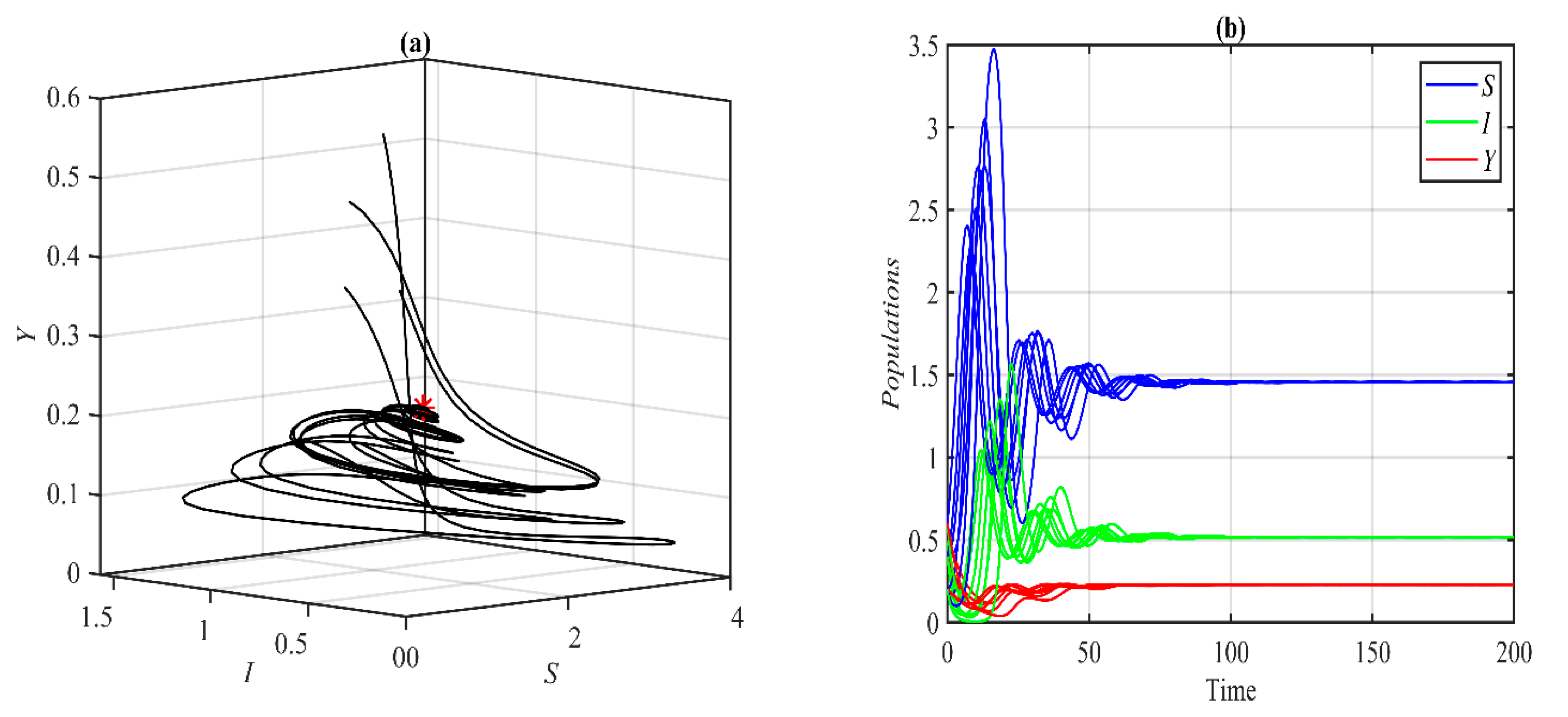
It is observed that for the above set of data, the system (1) approaches asymptotically to the P.E.P. that is determined by $m_4=\left(1.45,0.51,0.22\right)$ as presented in Figure 1 below.

Figure 1. The trajectories of system (1) using data set (49) and starting from different initial points approach asymptotically $m_4=\left(1.45,0.51,0.22\right)$: (a) 3D Phase plot. (b) Time series of solutions.

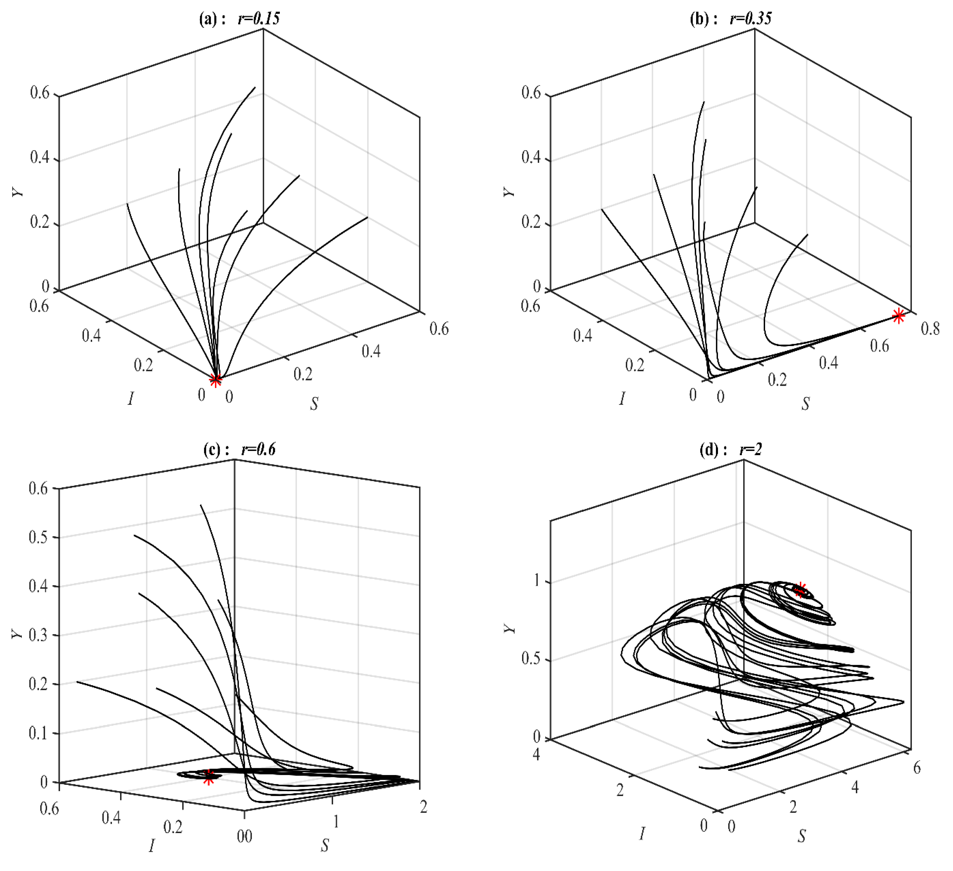
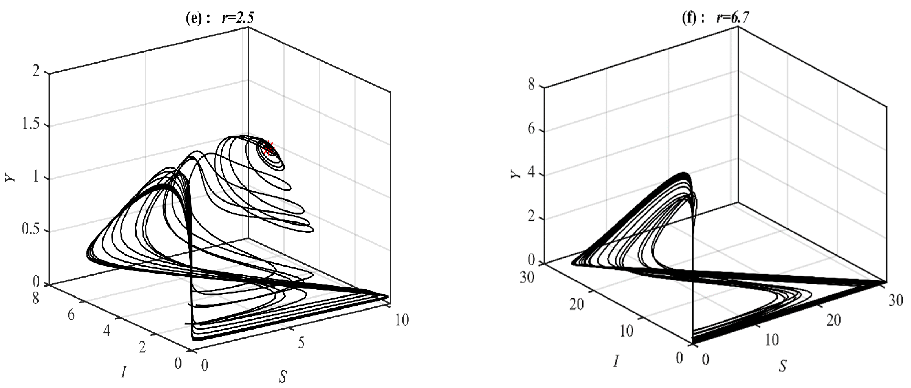
It is obvious from Figure 1 that system (1) has a unique asymptotically stable P.E.P. Now, the influence of varying the value of $r$ on the dynamic of the system (1) is studied, and the obtained results are presented at selected values in Figure 2. It is obtained that, for $r$ belongs to $\left(0,0.2\right)$, $\left[0.2,0.4\right]$, $\left(0.4,0.68\right)$, $\left[0.68,2.06\right)$, $\left[2.06,6.61\right]$, and $r\ge 6.62$, the system’s (1) solution approaches $m_0$, $m_1$, $m_2$, $m_4$, bistable between $m_4$ and 3D periodic attractor, and 3d periodic attractor, respectively.

Figure 2. The trajectories of system (1) using data set (49) with different values of $r$ and starting from various initial points. (a) Three-dimensional Phase plot converges $m_0$. (b) Three-dimensional Phase plot converges $m_1=\left(0.75,0,0\right)$. (c) Three-dimensional Phase plot converges $m_2=\left(1,0.4,0\right)$. (d) Three-dimensional Phase plot converges $m_4=\left(3.3,0.46,1.15\right)$. (e) Three-dimensional Phase plot for bistable between 3D periodic and $m_4=\left(4.38,0.45,1.69\right)$. (f) Three-dimensional Phase plot converges 3D periodic attractor.

According to Figure 2, there are five bifurcation points belonging to the range of $r,$ including the transcritical point. For the $\alpha$ to belong to $\left(0,0.13\right]$, $\left(0.13,0.42\right)$, $\left[0.42,0.8\right)$, and $\alpha \ge 0.8$, the solution of system (1) converges 3D periodic attractor, $m_4$, $m_2$, and $m_1$, see Figure 3 for the selected values of $\alpha$.

Figure 3. The trajectories of system (1) using data set (49) with different values of $\alpha$ and starting from various initial points. (a) Three-dimensional Phase plot converges 3D periodic attractor. (b) Three-dimensional Phase plot converges $m_4=\left(1.17,0.53,0.09\right)$. (c) Three-dimensional Phase plot converges $m_2=\left(1,0.37,0\right)$. (d) Three-dimensional Phase plot converges $m_1=\left(0.94,0,0\right)$.

According to Figure 3, there are three bifurcation points in the range of $\alpha$. Similar behaviors are obtained when varying the parameter $h_2$ as those obtained with $\alpha$.

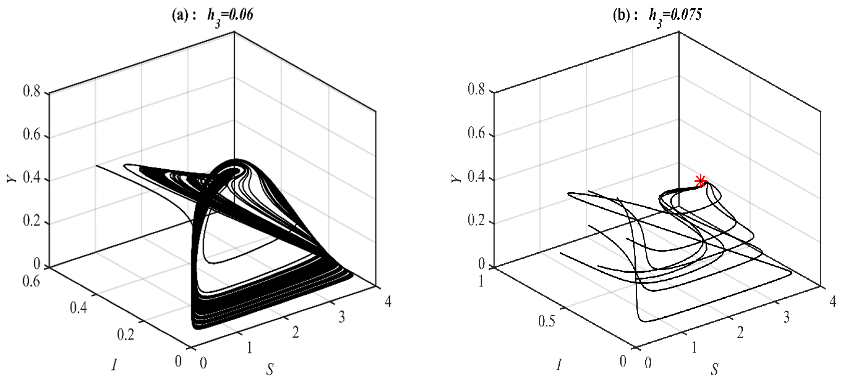
Now, the influence of varying the parameters $\theta$, $\mu$ and $b$ in the case of the system (1) having periodic dynamics is investigated in Figure 4, Figure 5 and Figure 6. It is obtained that for the data set (49) with $\alpha =0.1$ and $\theta$ belonging to $\left[0,0.9\right)$, and $\left[0.9,1\right]$ the solution converges 3D periodic attractor, and $m_4$ respectively. While for the data set (49) with $\alpha =0.1$ and $\mu$ belonging to $\left[0,11\right)$, and $\mu \ge 11$, the solution converges 3D periodic attractor, and $m_4$ respectively, see Figure 4 for the selected values of $\theta$, and $\mu$. On the other hand, for the data set (49) with $\alpha =0.1$ and varying $b$ as shown in Figure 5 and Figure 6.

Figure 4. The trajectories of system (1) using data set (49) with $\alpha =0.1$ and selected values of $\theta$, and $\mu$. (a) Three-dimensional Phase plot converges 3D periodic attractor. (b) Three-dimensional Phase plot converges $m_4=\left(3.67,0.45,1.33\right)$. (c) Three-dimensional Phase plot converges 3D periodic attractor. (d) Three-dimensional Phase plot converges $m_4=\left(3.83,0.45,1.42\right)$.

Figure 5. The trajectories of system (1) using data set (49) with $\alpha =0.1$ and selected values of $b$. (a) Three-dimensional Phase plot converges chaotic attractor. (b) Three-dimensional Phase plot converges $m_4=\left(1.85,0.71,0.42\right)$.

Figure 6. The bifurcation diagram as a function of $b\in \left(0,0.6\right)$ with the data set (49) and $\alpha =0.1$. (a) The trajectory of $S$ as a function of $b$. (b) The trajectory of $I$ as a function of $b$. (c) The trajectory of $Y$ as a function of $b$.

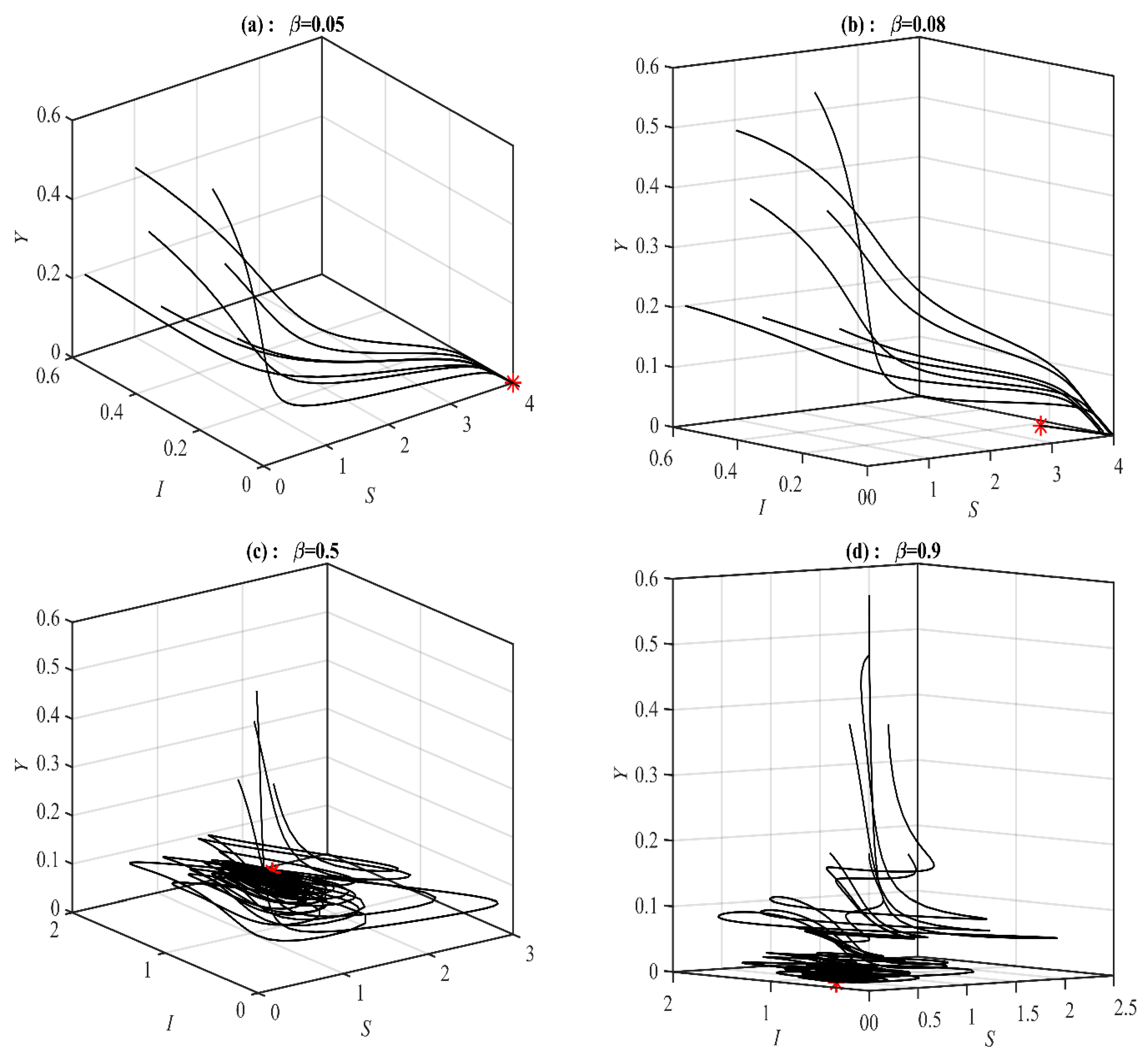
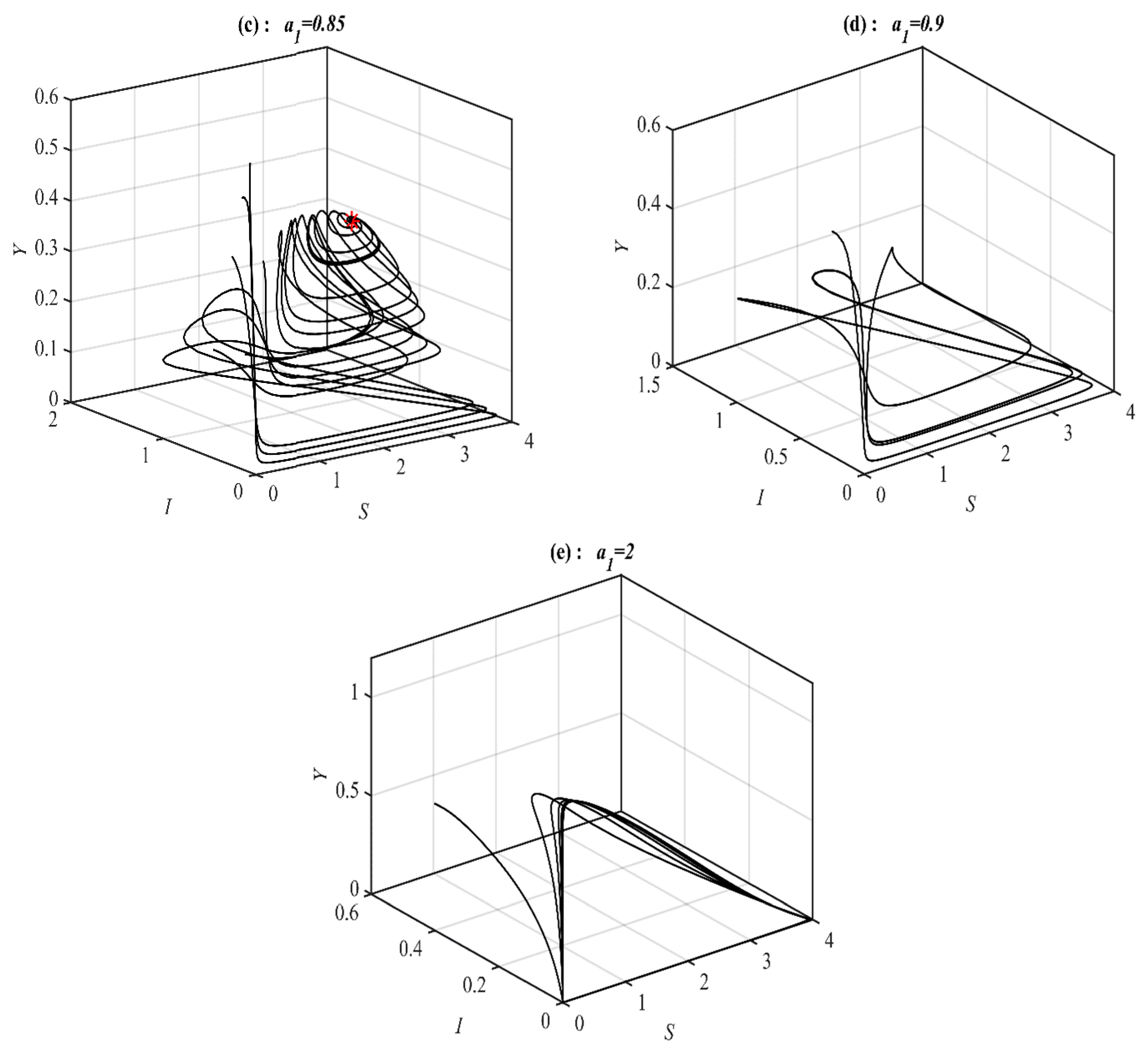
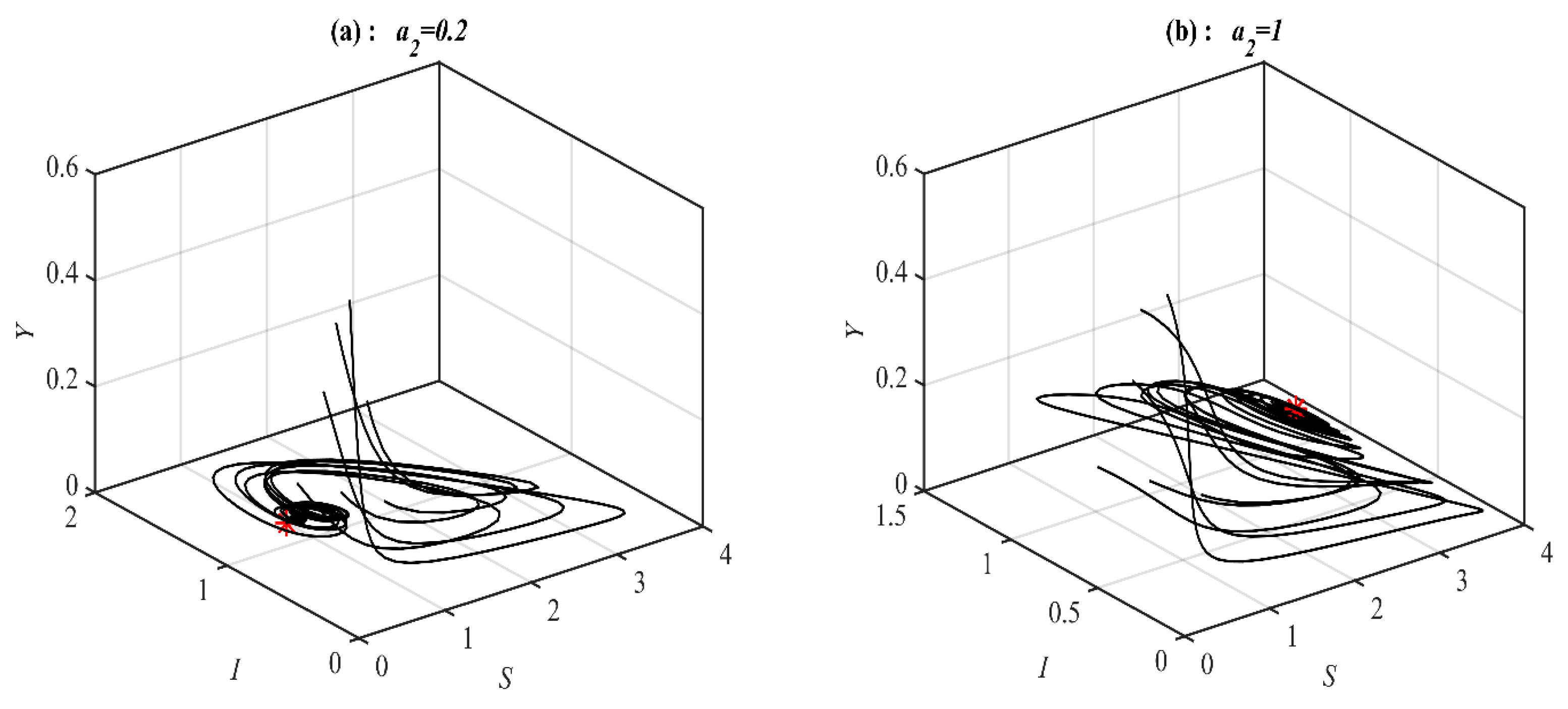
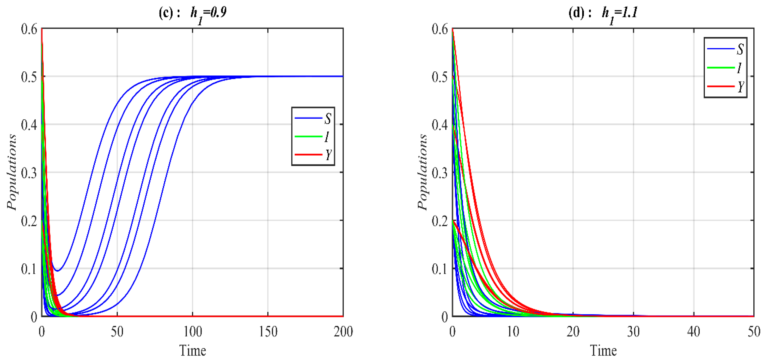
According to Figure 4, Figure 5 and Figure 6, the parameters $\theta$, $\mu$ and $b$ control the stability of the system (1). It is observed that the system converges to $m_1$, $m_2$, $m_4$, and $m_2$ when the parameter $\beta$ belongs to $\left(0,0.07\right]$, $\left(0.07,0.1\right)$, $\left[0.1,0.82\right]$, and $\beta >0.82$, respectively; see Figure 7 for selected values of $\beta$. However, the system converges, $m_2$, $m_4$, $m_3$, a 3D periodic attractor, and a 2D periodic attractor in the $SY$-plane when the parameter $a_1$ belongs to $\left(0,0.03\right]$, $\left(0.03,0.83\right)$, $\left[0.83,0.86\right]$, $\left[0.88,1.95\right)$, and $a_1\ge 1.95$, respectively, as shown in Figure 8 at the selected values. On the other hand, for $a_2$ in the ranges $\left(0,0.28\right]$ and $a_2>0.28$ it is noted that system (1) converges $m_2$ and $m_4$ respectively as presented in Figure 9 at typical values of $a_2$. However, for $d_1$ in the ranges $\left(0,0.64\right)$ and $d_1\ge 0.64$, it is noted that system (1) converges $m_4$ and $m_2$ respectively, as shown in Figure 10 at the typical value of $d_1$. Finally, it is obtained that varying the parameters $d_1$ and $d_2$ have a similar influence on the dynamics of the system (1).

Figure 7. The trajectories of system (1) using data set (49) with different values of $\beta$ and starting from various initial points. (a) Three-dimensional Phase plot converges $m_1=\left(4,0,0\right)$. (b) Three-dimensional Phase plot converges $m_2=\left(3.74,0.17,0\right)$. (c) Three-dimensional Phase plot converges $m_4=\left(0.8,0.58,0.16\right)$. (d) Three-dimensional Phase plot converges $m_2=\left(0.33,0.66,0\right)$.

Figure 8. The trajectories of system (1) using data set (49) with different values of $a_1$ and starting from various initial points. (a) Three-dimensional Phase plot converges $m_2=\left(1,1.19,0\right)$. (b) Three-dimensional Phase plot converges $m_4=\left(1.56,0.36,0.28\right)$. (c) Three-dimensional Phase plot converges $m_3=\left(1.5,0,0.46\right)$. (d) Three-dimensional Phase plot converges to a 3D periodic attractor. (e) Three-dimensional Phase plot converges to a 2D periodic attractor in the $SY$-plane.

Figure 9. The trajectories of system (1) using data set (49) with different values of $a_2$ and starting from various initial points. (a) Three-dimensional Phase plot converges $m_2=\left(1,1.2,0\right)$. (b) Three-dimensional Phase plot converges $m_4=\left(1.91,0.29,0.27\right)$.

Figure 10. The trajectories of system (1) using data set (49) with different values of $d_1$ and starting from various initial points. (a) Three-dimensional Phase plot converges $m_4=\left(2.19,0.48,0.09\right)$. (b) Three-dimensional Phase plot converges $m_2=\left(3,0.4,0\right)$.

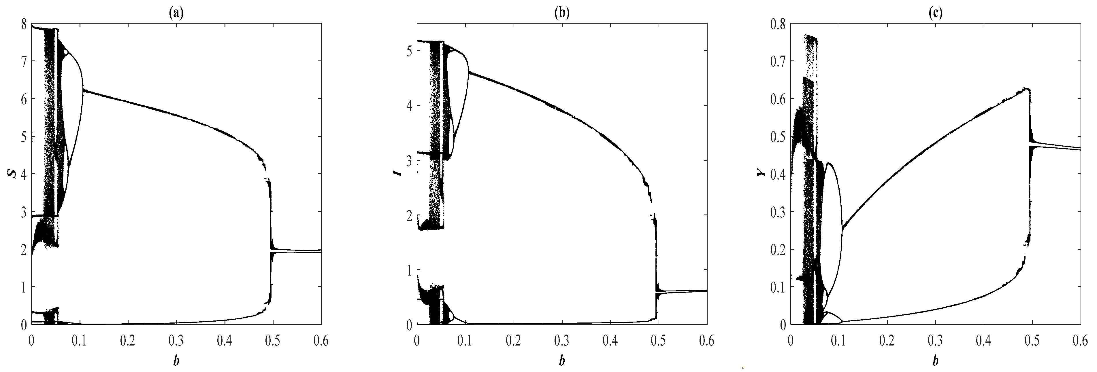
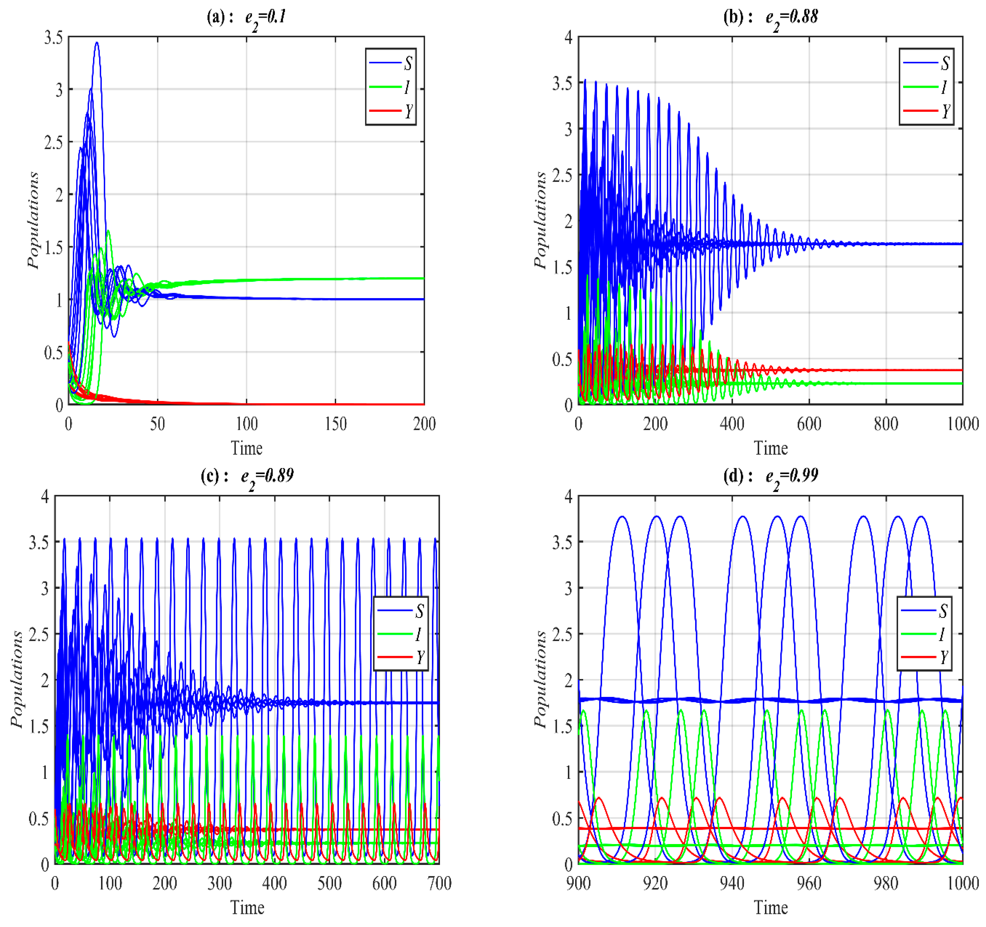
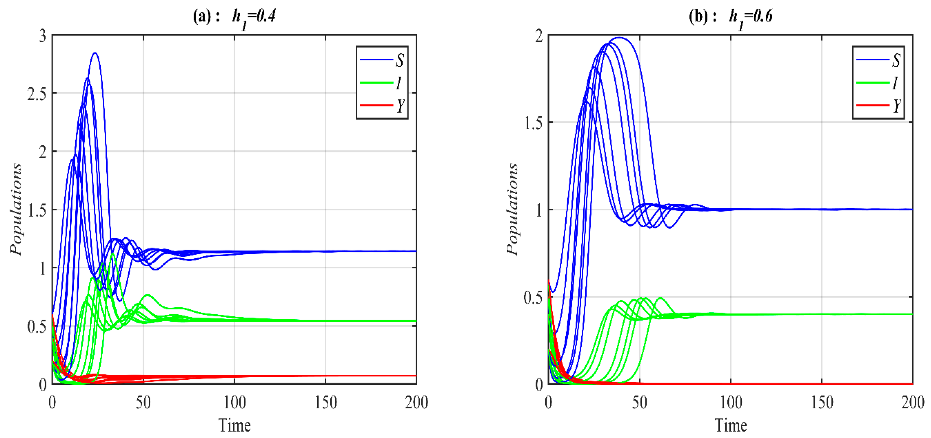
Now, it is found that the system converges to $m_4$, $m_3$, a 2D periodic attractor in the $SY$-plane, and a 3D periodic attractor when the parameter $e_1$ belongs to $\left[0,0.66\right)$, $\left[0.66,0.7\right]$, $\left(0.7,0.74\right]$, and $\left(0.74,1\right]$ respectively, see Figure 11 for selected values of $e_1$. However, the system converges, $m_2$, $m_4$, and bistable between the 3D periodic attractor and $m_4$ when the parameter $e_2$ belongs to $\left[0,0.18\right]$, $\left(0.18,0.89\right)$, and $\left[0.89,1\right]$, respectively, as shown in Figure 12 using selected values of $e_2$. On the other hand, for $h_1$ in the ranges $\left(0,0.53\right)$, $\left[0.53,0.8\right)$, $\left(0.8,1\right)$ and $h_1\ge 1$, it is noted that system (1) converges $m_4$, $m_2$, $m_1$, and $m_0$, respectively, as presented in Figure 13 at typical values of $h_1$. However, for $h_3$ in the ranges $\left(0,0.07\right)$, $\left[0.07,0.08\right]$, $\left(0.08,0.35\right]$ and $h_3>0.35$ it is noted that system (1) converges chaotic attractor, $m_3$, $m_4$, and $m_2$, respectively, as shown in Figure 14 at a typical value of $h_3$. Finally, the bifurcation diagram is given in Figure 15 shows clearly the existence of chaos in the range $h_3\in \left(0,0.07\right)$.

Figure 11. The trajectories of system (1) using data set (49) with different values of $e_1$ and starting from various initial points. (a) Three-dimensional Phase plot converges $m_4=\left(1.64,0.32,0.32\right)$. (b) Three-dimensional Phase plot converges $m_3=\left(1.5,0,0.64\right)$. (c) Three-dimensional Phase plot converges a 2D periodic attractor in the $SY$-plane. (d) Three-dimensional Phase plot converges to a 3D periodic attractor.

Figure 12. The trajectories of system (1) using data set (49) with different values of $e_2$ and starting from various initial points. (a) Time series of the solutions that converge $m_2=\left(1,1.19,0\right)$. (b) Time series of the solutions that converge $m_4=\left(1.74,0.22,0.37\right)$. (c) Time series of the solutions that represent bistable between a 3D periodic attractor in the $SY$-plane and $m_4=\left(1.74,0.22,0.37\right)$. (d) Time series of the solutions that represent bistable between a 3D periodic attractor in the $SY$-plane and $m_4=\left(1.75,0.2,0.39\right)$.

Figure 13. The trajectories of system (1) using data set (49) with different values of $h_1$ and starting from various initial points. (a) Time series of the solutions that converge $m_4=\left(1.14,0.54,0.07\right)$. (b) Time series of the solutions that converge $m_2=\left(1,0.4,0\right)$. (c) Time series of the solutions that converge $m_1=\left(0.5,0,0\right)$. (d) Time series of the solutions that converge $m_0=\left(0,0,0\right)$.

Figure 14. The trajectories of system (1) using data set (49) with different values of $h_3$ and starting from various initial points. (a) Three-dimensional Phase plot converges chaotic attractor. (b) Three-dimensional Phase plot converges $m_3=\left(1.4,0,0.66\right)$. (c) Three-dimensional Phase plot converges $m_4=\left(1.66,0.29,0.33\right)$ (d) Three-dimensional Phase plot converges $m_2=\left(1,1.2,0\right)$.

Figure 15. The bifurcation diagram as a function of $h_3\in \left(0,0.1\right)$ with the data set (49). (a) The trajectory of $S$ as a function of $h_3$. (b) The trajectory of $I$ as a function of $h_3$. (c) The trajectory of $Y$ as a function of $h_3$.

7. Conclusions

In this study, the mathematical formulation and investigation of the effect of fear on a harvested prey–predator system in the presence of the disease among the prey population are carried out. Due to the difference in prey speed between healthy and diseased prey, two different types of Holling’s functional responses are used. The proposed model’s solution characteristics are investigated. The equilibrium points that are biologically viable have all been identified. Each equilibrium point’s local and global stability requirements are identified. The system’s persistence requirements are computed. Near the equilibrium points, all conceivable local bifurcation types are investigated. It is observed that system (1) is seen to undergo a transcritical bifurcation near the A.E.P. However, near the P.F.E.P. and D.F.E.P., the system has a transcritical bifurcation if a certain condition is met; otherwise, the system has a pitchfork bifurcation. Finally, saddle-node bifurcation occurs near the P.E.P. if certain criteria are met.

Finally, using a hypothetical set of parameter values, numerical research is conducted to confirm the analytical evaluation results and specify the impact of changing the parameter values. Regarding the impact of changing the parameter values on the system’s dynamic, the following conclusions are reached numerically (1). System (1) exhibits a variety of behaviors, including stable point, periodic, bistable, and chaotic behavior, because it is extremely sensitive to changes in its parameter values. From the perspective of how the parameters affect the system’s dynamic, the parameters can be divided into three groups: stabilizing, destabilizing, and extinction. The system (1) is stabilized at the positive equilibrium point in the stabilizing group by raising the parameters (the degree of fear and the minimal cost of fear, the predator’s half-saturation constant, and the predator’s maximum attack rate on the infected prey). Increasing the parameters, however, in the destabilizing group creates a destabilizing system (1), and the solution approaches asymptotically to 3D periodic attractors (the susceptible prey’s intrinsic growth rate and the conversion rates of the susceptible and infected biomass to predator biomass). Finally, every other parameter in the system (1) belongs to the extinction group because, when increased, it results in the extinction of one or more species.

References

- Hsu, S.-B.; Hwang, T.-W.; Kuang, Y. Global analysis of the Michaelis–Menten type ratio-dependent predator–prey system. J. Math. Biol. 2001, 42, 489–506. [Google Scholar] [CrossRef] [PubMed]
- Naji, R.K.; Balasim, A.T. On the dynamical behavior of three species food web model. Chaos Solitons Fractals 2007, 34, 1636–1648. [Google Scholar] [CrossRef]
- Liu, X.; Lou, Y. Global dynamics of a predator–prey model. J. Math. Anal. Appl. 2010, 371, 323–340. [Google Scholar] [CrossRef]
- Naji, R.K.; Upadhyay, R.K.; Rai, V. Dynamical consequences of predator interference in a tri-trophic model food chain. Nonlinear Anal. Real World Appl. 2010, 11, 809–818. [Google Scholar] [CrossRef]
- Gonzalez-Olivares, E. Multiple limit cycles in a Gause type predator-prey model with Holling type III functional response and Allee effect on prey. Bull. Math. Biol. 2011, 73, 1378–1397. [Google Scholar] [CrossRef]
- Xiaolei, Y.; Fuqin, S. Global dynamics of a predator-prey model incorporating a constant prey refuge. Electron. J. Differ. Equ. 2013, 2013, 1–8. [Google Scholar]
- Llibre, J.; Xiao, D. Global Dynamics of a Lotka-Volterra Model with Two Predators Competing for One Prey. SIAM J. Appl. Math. 2014, 74, 434–453. [Google Scholar] [CrossRef]
- Xu, C.; Yuan, S.; Zhang, T. Global dynamics of a predator–prey model with defense mechanism for prey. Appl. Math. Lett. 2016, 62, 42–48. [Google Scholar] [CrossRef]
- Fakhry, N.H.; Naji, R.K. The dynamics of a square root prey-predator model with fear. Iraqi J. Sci. 2020, 61, 139–146. [Google Scholar] [CrossRef]
- Volterra, V. Fluctuations in the abundance of a species considered mathematically. Nature 1926, 118, 558–560. [Google Scholar] [CrossRef]
- Lotka, A.J. Elements of physical biology. Nature 1926, 21, 341–343. [Google Scholar] [CrossRef]
- Holling, S.C. Some characteristics of simple types of predation and parasitism. Can. Entomol. 1959, 91, 385–398. [Google Scholar] [CrossRef]
- Anderson, R.M.; May, R. The invasion, persistence, and spread of infectious diseases within animal and plant communities. Philos. Trans. R. Soc. B Biol. Sci. 1986, 314, 533–570. [Google Scholar] [CrossRef]
- Pal, A.K.; Samanta, G.P. Stability analysis of an eco-epidemiological model incorporating a prey refuge. Nonlinear Anal. Model. Control 2010, 15, 473–491. [Google Scholar] [CrossRef]
- Naji, R.K.; Mustafa, A.N. The Dynamics of an Eco-Epidemiological Model with Nonlinear Incidence Rate. J. Appl. Math. 2012, 2012, 852631. [Google Scholar] [CrossRef]
- Sahoo, B.; Poria, S. Diseased prey-predator model with general Holling type interactions. Appl. Math. Comput. 2014, 226, 83–100. [Google Scholar] [CrossRef]
- Jana, S.; Kar, T.K. Modeling and analysis of a prey-predator system with disease in the prey. Chaos Solitons Fractals 2013, 47, 42–53. [Google Scholar] [CrossRef]
- Bera, S.P.; Maiti, A.; Samanta, G.P. A Prey-predator Model with Infection in Both Prey and Predator. Filomat 2015, 29, 1753–1767. [Google Scholar] [CrossRef]
- Abdulghafour, A.S.; Naji, R.K. A Study of a Diseased Prey-Predator Model with Refuge in Prey and Harvesting from Predator. J. Appl. Math. 2018, 2018, 17. [Google Scholar] [CrossRef]
- Hugo, A.; Simanjilo, E. Analysis of an Eco-Epidemiological Model under Optimal Control Measures for Infected Prey. Appl. Appl. Math. Int. J. 2019, 14, 117–138. [Google Scholar]
- Ibrahim, H.A.; Naji, R.K. A Prey-Predator Model with Michael-Mentence Type of Predator Harvesting and Infectious Disease in Prey. Iraqi J. Sci. 2020, 61, 1146–1163. [Google Scholar] [CrossRef]
- Hussein, W.; Satar, H.A. The Dynamics of a Prey-Predator Model with Infectious Disease in Prey: Role of Media Coverage. Iraqi J. Sci. 2021, 62, 4930–4952. [Google Scholar] [CrossRef]
- Bezabih, A.F.; Edessa, G.K.; Rao, K.P. Ecoepidemiological Model and Analysis of Prey-Predator System. J. Appl. Math. 2021, 2021, 6679686. [Google Scholar] [CrossRef]
- Savadogo, A.; Sangaré, B.; Ouedraogo, H. A mathematical analysis of prey-predator population dynamics in the presence of an SIS infectious disease. Res. Math. 2022, 9, 2020399. [Google Scholar] [CrossRef]
- Ganguli, C.; Kar, T.K. Optimal harvesting of a prey-predator model with variable carrying capacity. Int. J. Biomath. 2017, 10, 1750069. [Google Scholar] [CrossRef]
- Raymond, C.; Hugo, A.; Kung’aro, M. Modeling Dynamics of Prey-Predator Fishery Model with Harvesting: A Bioeconomic Model. J. Appl. Math. 2019, 2019, 2601648. [Google Scholar] [CrossRef]
- Satar, H.A.; Naji, R.K. Stability and Bifurcation in a Prey–Predator–Scavenger System with Michaelis–Menten Type of Harvesting Function. Differ. Equ. Dyn. Syst. 2022, 30, 933–956. [Google Scholar] [CrossRef]
- Liu, C.; Zhang, Q.; Zhang, Y.; Duan, X. Bifurcation and control in a differential-algebraic harvested prey-predator model with stage structure for predator. Int. J. Bifurc. Chaos 2008, 18, 3159–3168. [Google Scholar] [CrossRef]
- Taylor, R. Predation; Chapman & Hall: New York, NY, USA, 1984. [Google Scholar]
- Lima, S.; Dill, L.M. Behavioral decisions made under the risk of predation: A review and prospectus. Can. J. Zool. 1990, 68, 619–640. [Google Scholar] [CrossRef]
- Wang, X.; Zanette, L.; Zou, X. Modelling the fear effect in predator-prey interactions. J. Math. Biol. 2016, 75, 1179–1204. [Google Scholar] [CrossRef]
- Wang, X.; Zou, X. Modeling the fear effect in predator-prey interactions with adaptive avoidance of predators. Bull. Math. Biol. 2017, 79, 13–25. [Google Scholar] [CrossRef] [PubMed]
- Das, A.; Samanta, G.P. Modeling the fear effect on a stochastic prey-predator system with additional food for the predator. J. Phys. A Math. Theor. 2018, 51, 465601. [Google Scholar] [CrossRef]
- Wang, J.; Cai, Y.; Fu, S.; Wang, W. The effect of the fear factor on the dynamics of a predator-prey model incorporating the prey refuge. Chaos 2019, 29, 83109. [Google Scholar] [CrossRef] [PubMed]
- Zhanga, H.; Cai, Y.; Fu, S.; Wan, W. Impact of the fear effect in a prey-predator model incorporating a prey refuge. Appl. Math. Comput. 2019, 356, 328–337. [Google Scholar] [CrossRef]
- Sarkar, K.; Khajanchi, S. Impact of fear effect on the growth of prey in a predator-prey interaction model. Ecol. Complex. 2020, 42, 100826. [Google Scholar] [CrossRef]
- Maghool, F.H.; Naji, R.K. The dynamics of a tritrophic Leslie-Gower food-web system with the effect of fear. J. Appl. Math. 2021, 2021, 2112814. [Google Scholar] [CrossRef]
- Abbas, Z.S.; Naji, R.K. Modeling and Analysis of the Influence of Fear on a Harvested Food Web System. Mathematics 2022, 10, 3300. [Google Scholar] [CrossRef]
- Al-Momen, S.; Naji, R.K. The dynamics of modified Leslie-Gower predator-prey model under the influence of nonlinear harvesting and fear effect. Iraqi J. Sci. 2022, 63, 259–282. [Google Scholar] [CrossRef]
- Hale, J.K. Theory of Functional Differential Equations; Springer: Heidelberg, Germany, 1977. [Google Scholar]
- Perko, L. Differential Equations and Dynamical Systems, 3rd ed.; Springer: New York, NY, USA, 2001. [Google Scholar]
Disclaimer/Publisher’s Note: The statements, opinions and data contained in all publications are solely those of the individual author(s) and contributor(s) and not of MDPI and/or the editor(s). MDPI and/or the editor(s) disclaim responsibility for any injury to people or property resulting from any ideas, methods, instructions or products referred to in the content. |
© 2023 by the authors. Licensee MDPI, Basel, Switzerland. This article is an open access article distributed under the terms and conditions of the Creative Commons Attribution (CC BY) license (https://creativecommons.org/licenses/by/4.0/).