Study of Dynamic Solutions for Human–Machine System with Human Error and Common-Cause Failure

Abstract

This work investigates a dynamic solution of human–machine systems with human error and common-cause failure. By means of functional analysis, it is proved that the semigroup generated by the underlying operator converges exponentially to a projection operator by analyzing the spectral property of the underlying operator, and the asymptotic expressions of the system’s time-dependent solutions are presented. We also provide numerical examples to illustrate the effects of different parameters on the system and the theoretical analysis’s validity.

1. Introduction

As modern technology becomes more advanced, the study of the reliability of HMS has become more significant, developing into an essential part of the research on reliability theory. The HMS is a general term for systems where the human is the subject and various types of machines are controlled. Due to the development of automation and microelectronics, the allocation of human–machine functions is continually shifting to the machine side. The high precision and performance of machines increase the importance of human work responsibility, and there is the risk of major accidents caused by HR. Additionally, machines are affected by external environmental contingencies, such as earthquakes, floods, fires, and so on. When these destructive contingencies occur, numerous components in the overall system fail simultaneously, which is known as CCF.

By studying the history of reliability theory, it is easy to see that many reliability problems have been solved by establishing reliability models in which the SVT plays an essential role. The SVT was first proposed by Cox [1] in 1955 and was first introduced into the reliability theory by Gaver [2]. Following this research approach, researchers such as Abbas and Kuo [3], Yang and Dhillon [4], Sridharan and Mohanavadivu [5], Asadzadeh and Azadeh [6], and Wang [7] studied various human–machine reparable systems.

In general, the mathematical model established by the SVT is described by a finite or infinite set of partial differential integral equations with integral boundary conditions. Therefore, obtaining exact solutions is quite challenging. Because of this, some papers on reliability models assume that TDS converges to SSS. However, they do not address whether or not this assumption is correct. In 2003, Gupur [8] was the first to apply $C_0$-semigroup theory to investigate the TDS of an HMS consisting of an active and a standby component by the SVT. The strong [9] and exponential [10] convergence of the TDS to its SSS is then obtained separately. Wang and Xu [11] examined the well-posedness and asymptotic behavior of the TDS of an HMS with two parallel working components and a standby component. As systems become more complex, these simple systems are no longer adequate for engineering needs. In addition, as equipment becomes more reliable, the contribution of human error to system problems is relatively more significant. HR and CCF are vital issues in system reliability. Therefore, Chung [12], Narmada and Jacob [13], Hajeeh [14], Liu et al. [15], Shneiderman [16], and others (see the references therein) have examined the reliability of systems with HR and CCF. Yang and Dhillon [4] established a complex HMS consisting of $n(n\ge 2)$ active components and $m(m\ge 2)$ standby components with HR and CCF. Xu et al. [17] identified that the above system exists with a unique TDS, and it converges to the SSS. Other than the above results, there are no further results on this model’s dynamic analysis.

In this paper, first of all, we study the spectral properties of the underlying operator and demonstrate that, in a strip region on the left-half complex plane, it has a maximum number of finitely many eigenvalues and has an algebraic multiplicity of 1, of which 0 is strictly the dominant eigenvalue. Then, we show that the semigroup generated by the underlying operator of the model is quasi-compact and it is exponentially convergent to a projection operator. By studying the essential growth bound of the operator semigroup, it is shown that 0 is a pole of order 1. These results give an explicit expression for the projection operator by the residue theorem of the operator form. Finally, we provide the asymptotic expressions of the TDS of the system.

2. Mathematical Model of the System

The assumptions and symbols associated with our mathematical model are as follows.

• In the system, there are n active components and m standby components.
• When one of the operating components fails, the standby component switches into operation; when all components fail, the system fails.
• A CCF or a HR can trigger system failure from any of the system operable states. ${\lambda }_{ci}$ represents the constant CCF rate from state i to state m + n + 1; ${\lambda }_{hi}$ denotes the constant critical HR rate from state i to state m + n + 2; for i = 0, 1, 2, …, m + n − 1.
• common-cause and other failure rates are constant. $r_i$ denotes the constant hardware failure rate of a unit in state i; i = 0, 1, 2, …, m + n − 1.
• The failed system repair times are arbitrarily distributed; ${\mu }_j\left(x\right)$ represents the system’s time-dependent repair rate when the system is in state j and satisfies ${\mu }_j\left(x\right)\ge 0,{\int }_0^{\infty }{\mu }_j\left(x\right)dx=\infty$ for j = m + n, m + n + 1, m + n + 2.
• The repaired component or system is as good as new. ${\mu }_i$ denotes the constant repair rate of a failed unit in state i, where i = 1, 2, …, m + n − 1.
• All failures including HR are statistically independent, and the switchover mechanism is perfect and instantaneous.

Based on the above assumptions and descriptions, the state transition diagram of the system Figure 1 can be presented as below.

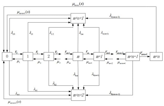
Figure 1. The state transition diagram of the system.

According to Yang and Dhillon [4], the following partial differential integral equations describe the mathematical model of the HMS with HR and CCF.

$$\begin{array}{cc}\hfill & \frac{\mathrm{d}{\mathsf{\Phi }}_0\left(\mathrm{t}\right)}{\mathrm{dt}}=-a_0{\mathsf{\Phi }}_0\left(\mathrm{t}\right)+{\mu }_1{\mathsf{\Phi }}_1\left(\mathrm{t}\right)+\sum _{j=\varrho }^{\varrho +2}{\int }_0^{\infty }{\mathsf{\Phi }}_j(x,\mathrm{t}){\mu }_j\left(x\right)\mathrm{d}x,\hfill \end{array}$$

(1)

$$\begin{array}{cc}\hfill & \frac{\mathrm{d}{\mathsf{\Phi }}_i\left(\mathrm{t}\right)}{\mathrm{d}\mathrm{t}}=r_{i-1}{\mathsf{\Phi }}_{i-1}\left(\mathrm{t}\right)-a_i{\mathsf{\Phi }}_i\left(\mathrm{t}\right)+{\mu }_{i+1}{\mathsf{\Phi }}_{i+1}\left(\mathrm{t}\right),i=1,2,\dots ,\varrho -2,\hfill \end{array}$$

(2)

$$\begin{array}{cc}\hfill & \frac{\mathrm{d}{\mathsf{\Phi }}_{\varrho -1}\left(\mathrm{t}\right)}{\mathrm{d}\mathrm{t}}=r_{\varrho -2}{\mathsf{\Phi }}_{\varrho -2}\left(\mathrm{t}\right)-a_{\varrho -1}{\mathsf{\Phi }}_{\varrho -1}\left(\mathrm{t}\right),\hfill \end{array}$$

(3)

$$\begin{array}{cc}\hfill & \frac{\partial {\mathsf{\Phi }}_j(x,\mathrm{t})}{\partial \mathrm{t}}+\frac{\partial {\mathsf{\Phi }}_j(x,\mathrm{t})}{\partial x}=-{\mu }_j\left(x\right){\mathsf{\Phi }}_j(x,\mathrm{t}),j=m+n,m+n+1,m+n+2,\hfill \end{array}$$

(4)

$$\begin{array}{cc}\hfill & {\mathsf{\Phi }}_{\varrho }(0,\mathrm{t})=r_{\varrho -1}{\mathsf{\Phi }}_{\varrho -1}\left(\mathrm{t}\right),\hfill \end{array}$$

(5)

$$\begin{array}{cc}\hfill & {\mathsf{\Phi }}_{\varrho +1}(0,\mathrm{t})=\sum _{i=0}^{\varrho -1}{\lambda }_{ci}{\mathsf{\Phi }}_i\left(\mathrm{t}\right),\hfill \end{array}$$

(6)

$${\mathsf{\Phi }}_{\varrho +2}(0,\mathrm{t})=\sum _{i=0}^{\varrho -1}{\lambda }_{hi}{\mathsf{\Phi }}_i\left(\mathrm{t}\right),$$

(7)

$$\begin{array}{c}{\mathsf{\Phi }}_0\left(0\right)=1,{\mathsf{\Phi }}_i\left(0\right)=0,i=1,2,\dots ,\varrho -1,\hfill \\ {\mathsf{\Phi }}_j(x,0)=0.\hfill \end{array}$$

(8)

where $(x,\mathrm{t})\in [0,\infty )\times [0,\infty ),$$a_0=r_0+{\lambda }_{c0}+{\lambda }_{h0},a_i=r_i+{\mu }_i+{\lambda }_{ci}+{\lambda }_{hi},i=1,2,\dots ,\varrho -1$ and $\varrho =m+n$. We use this denotation throughout the article.

$${\mathsf{\Phi }}_0\left(\mathrm{t}\right)=P\left\{\begin{array}{c}attime\mathrm{t},nworkingunitsandmstandbyunitsof\hfill \\ thesystemareingoodcondition\hfill \end{array}\right\},$$

$${\mathsf{\Phi }}_i\left(\mathrm{t}\right)=\left\{\begin{array}{c}P\left\{\begin{array}{c}nunitsworkingandm-iunitsonstandbyinthesystem\hfill \end{array}\right\},i\le m,\hfill \\ \\ P\left\{\begin{array}{c}\varrho -iunitsworkingandnounitsonstandbyinthesystem\hfill \end{array}\right\},i\ge m.\hfill \end{array}\right.$$

$$\begin{array}{cc}\hfill {\mathsf{\Phi }}_{\varrho }(x,\mathrm{t})& =P\left\{\begin{array}{c}attime\mathrm{t},thesystemfailsduetothefailureofallunits,\hfill \\ andtherepairtimeconsumedbyoneofthecomponentsisx\hfill \end{array}\right\},\hfill \\ \\ \hfill {\mathsf{\Phi }}_{\varrho +1}(x,\mathrm{t})& =P\left\{\begin{array}{c}attime\mathrm{t},thesystemfailsduetoCCF,\hfill \\ andtherepairtimeconsumedisx\hfill \end{array}\right\},\hfill \\ \\ \hfill {\mathsf{\Phi }}_{\varrho +2}(x,\mathrm{t})& =P\left\{\begin{array}{c}attimet,thesystemfailsduetoHR,\hfill \\ andtherepairtimeconsumedisx\hfill \end{array}\right\}.\hfill \end{array}$$

In the following, we introduce some notations:

$$\mathsf{\Gamma }=\left(\begin{array}{cccccccc}1& 0& 0& \cdots & 0& 0& 0& 0\\ 0& 0& 0& \cdots & 0& 0& 0& 0\\ ⋮& ⋮& ⋮& \ddots & ⋮& ⋮& ⋮& ⋮\\ 0& 0& 0& \cdots & 0& \\ 0& 0& 0& \cdots & r_{\varrho -1}& \\ {\lambda }_{c0}& {\lambda }_{c1}& {\lambda }_{c2}& \cdots & {\lambda }_{c\varrho -1}& & 0\\ {\lambda }_{h0}& {\lambda }_{h1}& {\lambda }_{h2}& \cdots & {\lambda }_{h\varrho -1}& \end{array}\right)$$

$$\left\{\begin{array}{c}{\mathfrak{B}}_j{f}_j\left(x\right)=-\frac{\mathrm{d}{f}_j\left(x\right)}{\mathrm{d}x}-{\mu }_j\left(x\right),f_j\in W^1[0,\infty );\hfill \\ {\varphi }_j{f}_j\left(x\right)={\int }_0^{\infty }{\mu }_j\left(x\right)f_j\left(x\right)\mathrm{d}x,f_j\in L^1[0,\infty ).\hfill \end{array}\right.$$

$$\left\{\begin{array}{c}{e}_j\left(x\right)=e^{-\eta x-{\int }_0^x{\mu }_j\left(\tau \right)\mathrm{d}\tau };\hfill \\ {\mathcal{E}}_j{g}_j\left(x\right)=e^{-\eta x-{\int }_0^x{\mu }_j\left(\tau \right)\mathrm{d}\tau }{\int }_0^x{g}_j\left(\xi \right)e^{\eta \xi +{\int }_0^{\xi }{\mu }_j\left(\tau \right)\mathrm{d}\tau }\mathrm{d}\xi ,\forall g\in L^1[0,\infty ).\hfill \end{array}\right.$$

Take the following Banach space $\mathrm{X}$ as a state space:

$$\mathrm{X}=\left\{\mathsf{\Phi }\left|\begin{array}{c}\mathsf{\Phi }\in {\mathbb{R}}^{\varrho }\times L^1[0,\infty )\times L^1[0,\infty )\times L^1[0,\infty )\hfill \\ \Vert \mathsf{\Phi }\Vert =\sum _{i=0}^{\varrho -1}|{\mathsf{\Phi }}_i|+\sum _{j=\varrho }^{\varrho +2}{\Vert {\mathsf{\Phi }}_j\Vert }_{L^1[0,\infty )}<\infty \hfill \end{array}\right.\right\}.$$

Define the operators and their domain.

$$D\left(\mathcal{H}\right)=\left\{\mathsf{\Phi }\in \mathrm{X}\left|\begin{array}{c}\frac{\mathrm{d}{\mathsf{\Phi }}_j\left(x\right)}{\mathrm{d}x}\in L^1[0,\infty ),{\mathsf{\Phi }}_j\left(x\right)areabsolutelycontinuous\hfill \\ {\displaystyle and\mathsf{\Phi }\left(0\right)=\mathsf{\Gamma }\mathsf{\Phi }\left(x\right)}\hfill \end{array}\right.\right\},$$

$$\mathcal{H}\left(\begin{array}{c}{\mathsf{\Phi }}_0\\ {\mathsf{\Phi }}_1\\ ⋮\\ {\mathsf{\Phi }}_{\varrho -1}\\ {\mathsf{\Phi }}_{\varrho }\\ {\mathsf{\Phi }}_{\varrho +1}\\ {\mathsf{\Phi }}_{\varrho +2}\end{array}\right)\left(x\right)=\left(\begin{array}{ccccccc}-a_0& 0& \cdots & 0& & & \\ 0& -a_1& \cdots & 0& & 0\\ 0& 0& \cdots & 0& & & \\ ⋮& ⋮& \ddots & ⋮& ⋮& ⋮& ⋮\\ 0& 0& \cdots & -a_{\varrho -1}& 0& 0& 0\\ & & \cdots & 0& {\mathfrak{B}}_{\varrho }& 0& 0\\ 0& & \cdots & 0& 0& {\mathfrak{B}}_{\varrho +1}& 0\\ & & \cdots & 0& 0& 0& {\mathfrak{B}}_{\varrho +2}\end{array}\right)\left(\begin{array}{c}{\mathsf{\Phi }}_0\\ {\mathsf{\Phi }}_1\\ ⋮\\ {\mathsf{\Phi }}_{\varrho -1}\\ {\mathsf{\Phi }}_{\varrho }\left(x\right)\\ {\mathsf{\Phi }}_{\varrho +1}\left(x\right)\\ {\mathsf{\Phi }}_{\varrho +2}\left(x\right)\end{array}\right),$$

$$\mathcal{M}\left(\begin{array}{c}{\mathsf{\Phi }}_0\\ {\mathsf{\Phi }}_1\\ ⋮\\ {\mathsf{\Phi }}_{\varrho -1}\\ {\mathsf{\Phi }}_{\varrho }\\ {\mathsf{\Phi }}_{\varrho +1}\\ {\mathsf{\Phi }}_{\varrho +2}\end{array}\right)\left(x\right)=\left(\begin{array}{ccccccccc}0& {\mu }_1& 0& \cdots & 0& 0& 0& 0& 0\\ r_0& 0& {\mu }_2& \cdots & 0& 0& 0& 0& 0\\ 0& r_1& 0& \ddots & 0& 0& 0& 0& 0\\ ⋮& ⋮& \ddots & \ddots & \ddots & ⋮& ⋮& ⋮& ⋮\\ 0& 0& 0& \cdots & 0& {\mu }_{\varrho -1}& 0& 0& 0\\ & & & \cdots & r_{\varrho -2}& & & & \\ & & & \cdots & 0& & & & \\ & 0& & \cdots & 0& & 0& & \\ & & & \cdots & 0& & & & \end{array}\right)\left(\begin{array}{c}{\mathsf{\Phi }}_0\\ {\mathsf{\Phi }}_1\\ ⋮\\ {\mathsf{\Phi }}_{\varrho -1}\\ {\mathsf{\Phi }}_{\varrho }\left(x\right)\\ {\mathsf{\Phi }}_{\varrho +1}\left(x\right)\\ {\mathsf{\Phi }}_{\varrho +2}\left(x\right)\end{array}\right),$$

$$\mathcal{S}\left(\begin{array}{c}{\mathsf{\Phi }}_0\\ {\mathsf{\Phi }}_1\\ ⋮\\ {\mathsf{\Phi }}_{\varrho -1}\\ {\mathsf{\Phi }}_{\varrho }\\ {\mathsf{\Phi }}_{\varrho +1}\\ {\mathsf{\Phi }}_{\varrho +2}\end{array}\right)\left(x\right)=\left(\begin{array}{c}\sum _{j=\varrho }^{\varrho +2}{\varphi }_j\\ 0\end{array}\right),D\left(\mathcal{M}\right)=D\left(\mathcal{S}\right)=X.$$

Then, (7) and (8) can be written as an abstract Cauchy problem: X:

$$\left\{\begin{array}{c}\frac{\mathrm{d}\mathsf{\Phi }\left(\mathrm{t}\right)}{\mathrm{d}\mathrm{t}}=(\mathcal{H}+\mathcal{M}+\mathcal{S})\mathsf{\Phi }\left(\mathrm{t}\right),\forall \mathrm{t}\in (0,\infty ),\hfill \\ \mathsf{\Phi }\left(0\right)=(1,0,0,\dots ,0).\hfill \end{array}\right.$$

(9)

3. Well-Posedness of (9)

Theorem 1. 

$\mathcal{H}+\mathcal{M}+\mathcal{S}$ generates a positive contraction $C_0$- semigroup $\mathcal{T}\left(\mathrm{t}\right)$ when $\overline{\mu }=\underset{x\in [0,\infty )}{sup}{\mu }_j\left(x\right)<\infty$.

The proof of Theorem 1 is omitted.

The dual space of X is given by

$$X^{\ast }=\left\{{\mathcal{Q}}^{\ast }\left|\begin{array}{c}{\mathcal{Q}}^{\ast }\in {\mathbb{R}}^{\varrho }\times L^{\infty }[0,\infty )\times L^{\infty }[0,\infty )\times L^{\infty }[0,\infty ),\hfill \\ \Vert |{\mathcal{Q}}^{\ast }\Vert |=max\left\{\underset{0⩽i⩽\varrho -1}{sup}|{{\mathcal{Q}}_i}^{\ast }|,\underset{\varrho ⩽j⩽\varrho +2}{sup}{\Vert {{\mathcal{Q}}_j}^{\ast }\Vert }_{L^{\infty }[0,\infty )}\right\}\hfill \end{array}\right.\right\}.$$

Obviously, $X^{\ast }$ is a Banach space. Let

$$W=\left\{\mathsf{\Phi }\in X\left|\begin{array}{c}\mathsf{\Phi }\left(x\right)=({\mathsf{\Phi }}_0,{\mathsf{\Phi }}_1,\dots ,{\mathsf{\Phi }}_{\varrho -1},{\mathsf{\Phi }}_{\varrho }\left(x\right),{\mathsf{\Phi }}_{\varrho +1}\left(x\right),{\mathsf{\Phi }}_{\varrho +2}\left(x\right)),\hfill \\ {\mathsf{\Phi }}_i⩾0,0⩽i⩽\varrho -1,{\mathsf{\Phi }}_j\left(x\right)⩾0,\forall x\in [0,\infty )\hfill \end{array}\right.\right\}.$$

Then, $W\subset X$, and Theorem 1 ensures that $\mathcal{T}\left(\mathrm{t}\right)W\subset W$. For $\mathsf{\Phi }\in D\left(\mathcal{H}\right)\bigcap W$, take ${\mathcal{Q}}^{\ast }\left(x\right)=\Vert \mathsf{\Phi }\Vert (1,1,\dots ,1)$; then, ${\mathcal{Q}}^{\ast }\in X^{\ast }$, and

$$\begin{array}{cc}\hfill & ⟨(\mathcal{H}+\mathcal{M}+\mathcal{S})\mathsf{\Phi },{\mathcal{Q}}^{\ast }⟩\hfill \\ \hfill & =\left\{-a_0{\mathsf{\Phi }}_0+{\mu }_1{\mathsf{\Phi }}_1+\sum _{j=\varrho }^{\varrho +2}{\int }_0^{\infty }{\mathsf{\Phi }}_j\left(x\right){\mu }_j\left(x\right)\mathrm{d}x\right\}\Vert \mathsf{\Phi }\Vert \hfill \\ \hfill & +\sum _{i=1}^{\varrho -2}\left\{r_{i-1}{\mathsf{\Phi }}_{i-1}-a_i{\mathsf{\Phi }}_i+{\mu }_{i+1}{\mathsf{\Phi }}_{i+1}\right\}\Vert \mathsf{\Phi }\Vert \hfill \\ \hfill & +\left\{r_{\varrho -2}{\mathsf{\Phi }}_{\varrho -2}-a_{\varrho -1}{\mathsf{\Phi }}_{\varrho -1}\right\}\Vert \mathsf{\Phi }\Vert \hfill \\ \hfill & +{\int }_0^{\infty }\left\{-\frac{\mathrm{d}{\mathsf{\Phi }}_{\varrho }\left(x\right)}{\mathrm{d}x}-{\mu }_{\varrho }\left(x\right){\mathsf{\Phi }}_{\varrho }\left(x\right)\right\}\Vert \mathsf{\Phi }\Vert \mathrm{d}x\hfill \\ \hfill & +{\int }_0^{\infty }\left\{-\frac{\mathrm{d}{\mathsf{\Phi }}_{\varrho +1}\left(x\right)}{\mathrm{d}x}-{\mu }_{\varrho +1}\left(x\right){\mathsf{\Phi }}_{\varrho +1}\left(x\right)\right\}\Vert \mathsf{\Phi }\Vert \mathrm{d}x\hfill \\ \hfill & +{\int }_0^{\infty }\left\{-\frac{\mathrm{d}{\mathsf{\Phi }}_{\varrho +2}\left(x\right)}{\mathrm{d}x}-{\mu }_{\varrho +2}\left(x\right){\mathsf{\Phi }}_{\varrho +2}\left(x\right)\right\}\Vert \mathsf{\Phi }\Vert \mathrm{d}x\hfill \\ \hfill & =-a_0{\mathsf{\Phi }}_0\Vert \mathsf{\Phi }\Vert +{\mu }_1{\mathsf{\Phi }}_1\Vert \mathsf{\Phi }\Vert +\sum _{j=\varrho }^{\varrho +2}\Vert \mathsf{\Phi }\Vert {\int }_0^{\infty }{\mathsf{\Phi }}_j\left(x\right){\mu }_j\left(x\right)\mathrm{d}x\hfill \\ \hfill & +\sum _{i=1}^{\varrho -2}\Vert \mathsf{\Phi }\Vert r_{i-1}{\mathsf{\Phi }}_{i-1}-\sum _{i=1}^{\varrho -2}\Vert \mathsf{\Phi }\Vert a_i{\mathsf{\Phi }}_i+\sum _{i=1}^{\varrho -2}\Vert \mathsf{\Phi }\Vert {\mu }_{i+1}{\mathsf{\Phi }}_{i+1}\hfill \\ \hfill & +r_{\varrho -2}{\mathsf{\Phi }}_{\varrho -2}\Vert \mathsf{\Phi }\Vert -a_{\varrho -1}{\mathsf{\Phi }}_{\varrho -1}\Vert \mathsf{\Phi }\Vert +\Vert \mathsf{\Phi }\Vert {\mathsf{\Phi }}_{\varrho }\left(0\right)\hfill \\ \hfill & -\Vert \mathsf{\Phi }\Vert \sum _{j=\varrho }^{\varrho +2}{\int }_0^{\infty }{\mathsf{\Phi }}_j\left(x\right){\mu }_j\left(x\right)\mathrm{d}x+\Vert \mathsf{\Phi }\Vert {\mathsf{\Phi }}_{\varrho +1}\left(0\right)+\Vert \mathsf{\Phi }\Vert {\mathsf{\Phi }}_{\varrho +2}\left(0\right)\hfill \\ \hfill & =-\sum _{i=0}^{\varrho -1}{a}_i{\mathsf{\Phi }}_i\Vert \mathsf{\Phi }\Vert +\sum _{i=0}^{\varrho -1}{r}_i{\mathsf{\Phi }}_i\Vert \mathsf{\Phi }\Vert +\sum _{i=0}^{\varrho -1}{\mu }_i{\mathsf{\Phi }}_i\Vert \mathsf{\Phi }\Vert \hfill \\ \hfill & +\sum _{i=0}^{\varrho -1}{\lambda }_{ci}{\mathsf{\Phi }}_i\Vert \mathsf{\Phi }\Vert +\sum _{i=0}^{\varrho -1}{\lambda }_{hi}{\mathsf{\Phi }}_i\Vert \mathsf{\Phi }\Vert \hfill \\ \hfill & =0.\hfill \end{array}$$

(10)

In (10), we use ${\mathsf{\Phi }}_j\in L^1[0,\infty )\Rightarrow {\mathsf{\Phi }}_j(\infty )=0.$

Equation (10) implies that $\mathcal{H}+\mathcal{M}+\mathcal{S}$ is a conservative operator with respect to the set $\mathsf{\Xi }\left(\mathsf{\Phi }\right)=\left\{{\mathcal{Q}}^{\ast }\in X^{\ast }\left|\begin{array}{c}⟨\mathsf{\Phi },{\mathcal{Q}}^{\ast }⟩={\Vert \mathsf{\Phi }\Vert }^2=\Vert |{\mathcal{Q}}^{\ast }{\Vert |}^2\hfill \end{array}\right.\right\}.$

Because of $\mathsf{\Phi }\left(0\right)\in D\left({\mathcal{H}}^2\right)\bigcap W$ and by using the Fattorini theorem [18], we obtain the following result.

Theorem 2. 

$\mathcal{T}\left(\mathrm{t}\right)$ is isometric for $\mathsf{\Phi }\left(0\right)$, i.e.,

$$\begin{array}{c}\hfill \parallel \mathcal{T}\left(\mathrm{t}\right)\mathsf{\Phi }\left(0\right)\parallel =\parallel \mathsf{\Phi }\left(0\right)\parallel ,\forall \mathrm{t}\in [0,\infty ).\end{array}$$

(11)

We can obtain the system’s well-posedness from Theorems 1 and 2.

Theorem 3. 

If $\overline{\mu }=sup{\mu }_j\left(x\right)<\infty$, then (9) has a unique positive TDS $\mathsf{\Phi }(x,\mathrm{t})$ satisfying

$$\parallel \mathsf{\Phi }(·,\mathrm{t})\parallel =1,\forall \mathrm{t}\in [0,\infty ).$$

4. Spectrum of the Operator $\mathcal{H}\mathbf{+}\mathcal{M}\mathbf{+}\mathcal{S}$

Lemma 1. 

If $0\le \underline{{\mu }_j}\le {\mu }_j\left(x\right)\le \overline{{\mu }_j}<\infty$, then $\mathcal{H}+\mathcal{M}+\mathcal{S}$ has at most finite eigenvalues in $\{\eta \in \mathbb{C}|-min\{\underline{{\mu }_{\varrho }},\underline{{\mu }_{\varrho +1}},\underline{{\mu }_{\varrho +2}}\}<\Re \eta \le 0\}$; the geometric multiplicity of each eigenvalue is one, and 0 is a strictly dominant eigenvalue.

Proof.  

$(\mathcal{H}+\mathcal{M}+\mathcal{S})\mathsf{\Phi }=\eta \mathsf{\Phi },$ i.e.,

$$\begin{array}{c}(a_0+\eta ){\mathsf{\Phi }}_0-{\mu }_1{\mathsf{\Phi }}_1=\sum _{j=\varrho }^{\varrho +2}{\int }_0^{\infty }{\mathsf{\Phi }}_j\left(x\right){\mu }_j\left(x\right)\mathrm{d}x,\hfill \end{array}$$

(12)

$$\begin{array}{c}(a_i+\eta ){\mathsf{\Phi }}_i=r_{i-1}{\mathsf{\Phi }}_{i-1}+{\mu }_{i+1}{\mathsf{\Phi }}_{i+1},i=1,2,\dots ,\varrho -2,\hfill \end{array}$$

(13)

$$\begin{array}{c}(a_{\varrho -1}+\eta ){\mathsf{\Phi }}_{\varrho -1}=r_{\varrho -2}{\mathsf{\Phi }}_{\varrho -2},\hfill \end{array}$$

(14)

$$\begin{array}{c}\frac{d{\mathsf{\Phi }}_j\left(x\right)}{dx}=-(\eta +{\mu }_j\left(x\right)){\mathsf{\Phi }}_j\left(x\right),\hfill \end{array}$$

(15)

$$\begin{array}{c}{\mathsf{\Phi }}_{\varrho }\left(0\right)=r_{\varrho -1}{\mathsf{\Phi }}_{\varrho -1},\hfill \end{array}$$

(16)

$$\begin{array}{c}{\mathsf{\Phi }}_{\varrho +1}\left(0\right)=\sum _{i=0}^{\varrho -1}{\lambda }_{ci}{\mathsf{\Phi }}_i,\hfill \end{array}$$

(17)

$$\begin{array}{c}{\mathsf{\Phi }}_{\varrho +2}\left(0\right)=\sum _{i=0}^{\varrho -1}{\lambda }_{hi}{\mathsf{\Phi }}_i.\hfill \end{array}$$

(18)

By solving (15), we have

$$\begin{array}{c}\hfill {\mathsf{\Phi }}_j\left(x\right)={\mathsf{\Phi }}_j\left(0\right)e_j\left(x\right),\end{array}$$

(19)

By substituting (16)–(18) into (19), we deduce

$${\mathsf{\Phi }}_{\varrho }\left(x\right)=r_{\varrho -1}{\mathsf{\Phi }}_{\varrho -1}{e}_{\varrho }\left(x\right),$$

(20)

$${\mathsf{\Phi }}_{\varrho +1}\left(x\right)=\sum _{i=0}^{\varrho -1}{\lambda }_{ci}{\mathsf{\Phi }}_i{e}_{\varrho +1}\left(x\right),$$

(21)

$${\mathsf{\Phi }}_{\varrho +2}\left(x\right)=\sum _{i=0}^{\varrho -1}{\lambda }_{hi}{\mathsf{\Phi }}_i{e}_{\varrho +2}\left(x\right).$$

(22)

From (13) and (14), we obtain

$$\begin{array}{c}\hfill \left(\begin{array}{cccccc}{a}_1+\eta & -{\mu }_2& 0& \cdots & 0& 0\\ -r_1& a_2+\eta & -{\mu }_3& \cdots & 0& 0\\ 0& -r_2& a_3+\eta & \cdots & 0& 0\\ ⋮& ⋮& ⋮& ⋮& ⋮& ⋮\\ 0& 0& 0& \cdots & -r_{\varrho -2}& a_{\varrho -1}+\eta \end{array}\right)\left(\begin{array}{c}{\mathsf{\Phi }}_1\\ {\mathsf{\Phi }}_2\\ {\mathsf{\Phi }}_3\\ ⋮\\ {\mathsf{\Phi }}_{\varrho -1}\end{array}\right)=\left(\begin{array}{c}{r}_0{\mathsf{\Phi }}_0\\ 0\\ 0\\ ⋮\\ 0\end{array}\right)\end{array}$$

By Cramer’s rule, we have

$${\mathsf{\Phi }}_i=\frac{|U_i|}{|U|}{\mathsf{\Phi }}_0,i=1,2,\dots ,\varrho -1.$$

(23)

Here, U is the coefficient matrix of the above equations, and $U_i$ is the matrix where the i column of the coefficient matrix is replaced by the following vector:

$$\left(r_0,0,0,\dots ,0\right).$$

By inserting (20)–(23) into (12), we obtain

$$I\left(\eta \right){\mathsf{\Phi }}_0=0,$$

(24)

where

$$\begin{array}{cc}\hfill I\left(\eta \right)=& a_0+\eta -{\mu }_1\frac{|U_1|}{|U|}-r_{\varrho -1}\frac{|U_{\varrho -1}|}{|U|}{\varphi }_{\varrho }{e}_{\varrho }\left(x\right)\hfill \\ \hfill & -\sum _{i=0}^{\varrho -1}{\lambda }_{ci}\frac{|U_i|}{|U|}{\varphi }_{\varrho +1}{e}_{\varrho +1}\left(x\right)-\sum _{i=0}^{\varrho -1}{\lambda }_{hi}\frac{|U_i|}{|U|}{\varphi }_{\varrho +2}{e}_{\varrho +2}\left(x\right),\hfill \end{array}$$

and $U_0=U$.

If ${\mathsf{\Phi }}_0=0$, then (20)–(23) imply ${\mathsf{\Phi }}_i=0,{\mathsf{\Phi }}_j\left(x\right)=0(i=0,1,\dots ,\varrho -1)$; that is to say, $\mathsf{\Phi }\left(x\right)=(0,0,\dots ,0)$. Thus, $\eta$ is not an eigenvalue of $\mathcal{H}+\mathcal{M}+\mathcal{S}$.

If ${\mathsf{\Phi }}_0\ne 0$, then (24) gives

$$I\left(\eta \right)=0.$$

(25)

That is to say,

$$I\left(\eta \right)=0\iff {\mathsf{\Phi }}_0\ne 0.$$

(26)

By (20)–(23) and the condition of Lemma 1 we estimate

$$\begin{array}{cc}\hfill \Vert \mathsf{\Phi }\Vert & =|{\mathsf{\Phi }}_0|+|{\mathsf{\Phi }}_1|+\dots +|{\mathsf{\Phi }}_{\varrho -1}|+\sum _{j=\varrho }^{\varrho +2}{\Vert {\mathsf{\Phi }}_j\Vert }_{L^1[0,\infty )}\hfill \\ \hfill & =\left(1+\sum _{i=1}^{\varrho -1}\frac{|U_i|}{|U|}\right)|{\mathsf{\Phi }}_0|+{\int }_0^{\infty }{r}_{\varrho -1}|{\mathsf{\Phi }}_{\varrho -1}|e_{\varrho }\left(x\right)\mathrm{d}x\hfill \\ \hfill & +{\int }_0^{\infty }\sum _{i=0}^{\varrho -1}{\lambda }_{ci}|{\mathsf{\Phi }}_i|e_{\varrho +1}\left(x\right)\mathrm{d}x+{\int }_0^{\infty }\sum _{i=0}^{\varrho -1}{\lambda }_{hi}|{\mathsf{\Phi }}_i|e_{\varrho +2}\left(x\right)\mathrm{d}x\hfill \\ \hfill & \le \left(1+\sum _{i=1}^{\varrho -1}\frac{|U_i|}{|U|}\right)|{\mathsf{\Phi }}_0|+r_{\varrho -1}\frac{|U_{\varrho -1}|}{|U|}|{\mathsf{\Phi }}_0|{\int }_0^{\infty }{e}^{-(\Re \eta +\underline{{\mu }_{\varrho }})x}\mathrm{d}x\hfill \\ \hfill & +\sum _{i=0}^{\varrho -1}{\lambda }_{ci}\frac{|U_i|}{|U|}|{\mathsf{\Phi }}_0|{\int }_0^{\infty }{e}^{-(\Re \eta +\underline{{\mu }_{\varrho +1}})x}\mathrm{d}x\hfill \\ \hfill & +\sum _{i=0}^{\varrho -1}{\lambda }_{hi}\frac{|U_i|}{|U|}|{\mathsf{\Phi }}_0|{\int }_0^{\infty }{e}^{-(\Re \eta +\underline{{\mu }_{\varrho +2}})x}\mathrm{d}x\hfill \\ \hfill & =|{\mathsf{\Phi }}_0|[1+\sum _{i=1}^{\varrho -1}\frac{|U_i|}{|U|}+r_{\varrho -1}\frac{|U_{\varrho -1}|}{|U|(\Re \eta +\underline{{\mu }_{\varrho }})}\hfill \\ \hfill & +\sum _{i=0}^{\varrho -1}{\lambda }_{ci}\frac{|U_i|}{|U|(\Re \eta +\underline{{\mu }_{\varrho +1}})}+\sum _{i=0}^{\varrho -1}{\lambda }_{hi}\frac{|U_i|}{|U|(\Re \eta +\underline{{\mu }_{\varrho +2}})}].\hfill \end{array}$$

(27)

By (26) and (27), it is not difficult to know that all zeros of $I\left(\eta \right)$ in

$$\Delta =\{\eta \in \mathbb{C}|-min\{\underline{{\mu }_{\varrho }},\underline{{\mu }_{\varrho +1}},\underline{{\mu }_{\varrho +2}}\}<\Re \eta \le 0\}$$

are eigenvalues of $\mathcal{H}+\mathcal{M}+\mathcal{S}$. Since $I\left(\eta \right)$ is analytic in $\Delta$, it follows that $I\left(\eta \right)$ has, at most, countable isolated zero points in $\Delta$ from the zero-point theorem of the analytic function.

In the following, we verify the above results. If $I\left(\eta \right)$ has infinitely many zero points in $\Delta$, and we assume that they are ${\eta }_l={\alpha }_l+i{\beta }_l\in \Delta ,{\alpha }_l\in (-min\{\underline{{\mu }_{\varrho }},\underline{{\mu }_{\varrho +1}},\underline{{\mu }_{\varrho +2}}\},0],{\beta }_l\in \mathbb{R}$, then we know that there is a convergent subsequence by the Bolzano–Weierstrass theorem. Without losing generality, assume ${\eta }_k={\alpha }_k+i{\beta }_k$ such that $\underset{k\to \infty }{lim}{\alpha }_k=\alpha \in (-min\{\underline{{\mu }_{\varrho }},\underline{{\mu }_{\varrho +1}},\underline{{\mu }_{\varrho +2}}\},0]$, $\underset{k\to \infty }{lim}|{\beta }_k|=\infty ,I\left({\eta }_k\right)=0,\forall k\ge 1.$ By inserting ${\eta }_k={\alpha }_k+i{\beta }_k$ into (25), we obtain

$$\begin{array}{c}{a}_0+{\alpha }_k+i{\beta }_k-{\mu }_1\frac{|U_1|}{|U|}\hfill \\ -r_{\varrho -1}\frac{|U_{\varrho -1}|}{|U|}{\int }_0^{\infty }{\mu }_{\varrho }\left(x\right)e^{-({\alpha }_k+i{\beta }_k)x-{\int }_0^x{\mu }_{\varrho }\left(\tau \right)\mathrm{d}\tau }\mathrm{d}x\hfill \\ -\sum _{i=0}^{\varrho -1}{\lambda }_{ci}\frac{|U_i|}{|U|}{\int }_0^{\infty }{\mu }_{\varrho +1}\left(x\right)e^{-({\alpha }_k+i{\beta }_k)x-{\int }_0^x{\mu }_{\varrho +1}\left(\tau \right)\mathrm{d}\tau }\mathrm{d}x\hfill \\ -\sum _{i=0}^{\varrho -1}{\lambda }_{hi}\frac{|U_i|}{|U|}{\int }_0^{\infty }{\mu }_{\varrho +2}\left(x\right)e^{-({\alpha }_k+i{\beta }_k)x-{\int }_0^x{\mu }_{\varrho +2}\left(\tau \right)\mathrm{d}\tau }\mathrm{d}x=0\hfill \\ ⟹\hfill \\ a_0+{\alpha }_k+i{\beta }_k-{\mu }_1\frac{|U_1|}{|U|}\hfill \\ -r_{\varrho -1}\frac{|U_{\varrho -1}|}{|U|}\times {\int }_0^{\infty }{\mu }_{\varrho }\left(x\right)e^{-{\alpha }_{k}x-{\int }_0^x{\mu }_{\varrho }\left(\tau \right)\mathrm{d}\tau }[cos\left({\beta }_{k}x\right)-isin\left({\beta }_{k}x\right)]\mathrm{d}x\hfill \\ -\sum _{i=0}^{\varrho -1}{\lambda }_{ci}\frac{|U_i|}{|U|}\times {\int }_0^{\infty }{\mu }_{\varrho +1}\left(x\right)e^{-{\alpha }_{k}x-{\int }_0^x{\mu }_{\varrho +1}\left(\tau \right)\mathrm{d}\tau }[cos\left({\beta }_{k}x\right)-isin\left({\beta }_{k}x\right)]\mathrm{d}x\hfill \\ -\sum _{i=0}^{\varrho -1}{\lambda }_{hi}\frac{|U_i|}{|U|}\times {\int }_0^{\infty }{\mu }_{\varrho +2}\left(x\right)e^{-{\alpha }_{k}x-{\int }_0^x{\mu }_{\varrho +2}\left(\tau \right)\mathrm{d}\tau }[cos\left({\beta }_{k}x\right)-isin\left({\beta }_{k}x\right)]\mathrm{d}x=0\hfill \\ ⟹\hfill \\ a_0+{\alpha }_k-{\mu }_1\frac{|U_1|}{|U|}\hfill \\ -r_{\varrho -1}\frac{|U_{\varrho -1}|}{|U|}{\int }_0^{\infty }{\mu }_{\varrho }\left(x\right)e^{-{\alpha }_{k}x-{\int }_0^x{\mu }_{\varrho }\left(\tau \right)\mathrm{d}\tau }cos\left({\beta }_{k}x\right)\mathrm{d}x\hfill \\ -\sum _{i=0}^{\varrho -1}{\lambda }_{ci}\frac{|U_i|}{|U|}{\int }_0^{\infty }{\mu }_{\varrho +1}\left(x\right)e^{-{\alpha }_{k}x-{\int }_0^x{\mu }_{\varrho +1}\left(\tau \right)\mathrm{d}\tau }cos\left({\beta }_{k}x\right)\mathrm{d}x\hfill \\ -\sum _{i=0}^{\varrho -1}{\lambda }_{hi}\frac{|U_i|}{|U|}{\int }_0^{\infty }{\mu }_{\varrho +2}\left(x\right)e^{-{\alpha }_{k}x-{\int }_0^x{\mu }_{\varrho +2}\left(\tau \right)\mathrm{d}\tau }cos\left({\beta }_{k}x\right)\mathrm{d}x=0,\hfill \end{array}$$

(28)

$$\begin{array}{c}{\beta }_k+r_{\varrho -1}\frac{|U_{\varrho -1}|}{|U|}{\int }_0^{\infty }{\mu }_{\varrho }\left(x\right)e^{-{\alpha }_{k}x-{\int }_0^x{\mu }_{\varrho }\left(\tau \right)\mathrm{d}\tau }sin\left({\beta }_{k}x\right)\mathrm{d}x\hfill \\ +\sum _{i=0}^{\varrho -1}{\lambda }_{ci}\frac{|U_i|}{|U|}{\int }_0^{\infty }{\mu }_{\varrho +1}\left(x\right)e^{-{\alpha }_{k}x-{\int }_0^x{\mu }_{\varrho +1}\left(\tau \right)\mathrm{d}\tau }sin\left({\beta }_{k}x\right)\mathrm{d}x\hfill \\ +\sum _{i=0}^{\varrho -1}{\lambda }_{hi}\frac{|U_i|}{|U|}{\int }_0^{\infty }{\mu }_{\varrho +2}\left(x\right)e^{-{\alpha }_{k}x-{\int }_0^x{\mu }_{\varrho +2}\left(\tau \right)\mathrm{d}\tau }sin\left({\beta }_{k}x\right)\mathrm{d}x=0.\hfill \end{array}$$

(29)

By ${\eta }_k\in \Delta$ and the Riemann–Lebesgue theorem, we know that

$$\underset{k\to \infty }{lim}{\int }_0^{\infty }{\mu }_j\left(x\right)e^{-{\alpha }_{k}x-{\int }_0^x{\mu }_j\left(\tau \right)\mathrm{d}\tau }cos\left({\beta }_{k}x\right)\mathrm{d}x=0,$$

(30)

$$\underset{k\to \infty }{lim}{\int }_0^{\infty }{\mu }_j\left(x\right)e^{-{\alpha }_{k}x-{\int }_0^x{\mu }_j\left(\tau \right)\mathrm{d}\tau }sin\left({\beta }_{k}x\right)\mathrm{d}x=0.$$

(31)

From (29)–(31) and taking the limit $k\to \infty$ in (29), we obtain that $\infty =0$. Obviously, this is a contradiction. Therefore, $I\left(\eta \right)$ has at most finite zero points in $\Delta$; in other words, $\mathcal{H}+\mathcal{M}+\mathcal{S}$ has finite eigenvalues at most in $\Delta$. Furthermore, according to (20)–(23), the eigenvectors corresponding to each $\eta$ generate a linear space of one dimension. That is, the geometric multiplicity of each $\eta$ is one. □

Remark 1. 

It is not difficult to prove that $I\left(0\right)=0$. Hence, 0 is the eigenvalue of $\mathcal{H}+\mathcal{M}+\mathcal{S}$ with a geometric multiplicity of one. Because $\mathcal{H}+\mathcal{M}+\mathcal{S}$ has finite eigenvalues and the real part of all non-zero eigenvalues is strictly less than 0 in Δ, 0 is a strictly dominant eigenvalue of $\mathcal{H}+\mathcal{M}+\mathcal{S}$.

Proof. 

when $\eta =0$,

$$\begin{array}{cc}\hfill I\left(0\right)& =a_0-{\mu }_1\frac{|U_1^0|}{|U^0|}-r_{\varrho -1}\frac{|U_{\varrho -1}^0|}{|U^0|}-\sum _{i=0}^{\varrho -1}{\lambda }_{ci}\frac{|U_i^0|}{|U^0|}-\sum _{i=0}^{\varrho -1}{\lambda }_{hi}\frac{|U_i^0|}{|U^0|}\hfill \\ \hfill & =a_0-{\lambda }_{c0}-{\lambda }_{h0}-\sum _{i=2}^{\varrho -2}(a_i-r_i-{\mu }_i)\frac{|U_i^0|}{|U^0|}-(a_1-r_1)\frac{|U_1^0|}{|U^0|}-(a_{\varrho -1}-{\mu }_{\varrho -1})\frac{|U_{\varrho -1}^0|}{|U^0|},\hfill \end{array}$$

(32)

where

$$\begin{array}{c}\hfill U^0=\left(\begin{array}{cccccc}{a}_1& -{\mu }_2& 0& \cdots & 0& 0\\ -r_1& a_2& -{\mu }_3& \cdots & 0& 0\\ 0& -r_2& a_3& \cdots & 0& 0\\ ⋮& ⋮& ⋮& ⋮& ⋮& ⋮\\ 0& 0& 0& \cdots & -r_{\varrho -2}& a_{\varrho -1}\end{array}\right)\end{array}$$

$U_i^0$ denotes the matrix where the i column of $U^0$ is replaced by the vector

$$\left(r_0,0,0,\dots ,0\right).$$

According to the properties of the determinant, we obtain

$$\begin{array}{cc}\hfill & r_{\varrho -2}\frac{|U_{\varrho -2}^0|}{|U^0|}-a_{\varrho -1}\frac{|U_{\varrho -1}^0|}{|U^0|}=0,\hfill \\ \hfill & r_{i-1}\frac{|U_{i-1}^0|}{|U^0|}-a_i\frac{|U_i^0|}{|U^0|}+{\mu }_{i+1}\frac{|U_{i+1}^0|}{|U^0|}=0,i=2,3,\dots ,\varrho -2.\hfill \end{array}$$

Then, (32) becomes

$$\begin{array}{cc}\hfill I\left(0\right)& =a_0-{\lambda }_{c0}-{\lambda }_{h0}-a_1\frac{|U_1^0|}{|U^0|}-{\mu }_2\frac{|U_1^0|}{|U^0|}\hfill \\ \hfill & =a_0-{\lambda }_{c0}-{\lambda }_{h0}-r_0\hfill \\ \hfill & =0.\hfill \end{array}$$

□

Lemma 2. 

${(\mathcal{H}+\mathcal{M}+\mathcal{S})}^{\ast }$ is given by

$${(\mathcal{H}+\mathcal{M}+\mathcal{S})}^{\ast }{\mathcal{Q}}^{\ast }=(C+N+V){\mathcal{Q}}^{\ast },\forall {\mathcal{Q}}^{\ast }\in D\left(C\right)$$

where

$$\begin{array}{cc}\hfill C{\mathcal{Q}}^{\ast }\left(x\right)& =\left(\begin{array}{cccccc}-a_0& \cdots & 0& 0& 0& 0\\ 0& \cdots & 0& 0& 0& 0\\ ⋮& \ddots & ⋮& ⋮& ⋮& ⋮\\ 0& \cdots & -a_{\varrho -1}& 0& 0& 0\\ 0& \cdots & 0& \frac{\mathrm{d}}{\mathrm{d}x}-{\mu }_{\varrho }\left(x\right)& 0& 0\\ 0& \cdots & 0& 0& \frac{\mathrm{d}}{\mathrm{d}x}-{\mu }_{\varrho +1}\left(x\right)& 0\\ 0& \cdots & 0& 0& 0& \frac{\mathrm{d}}{\mathrm{d}x}-{\mu }_{\varrho +2}\left(x\right)\end{array}\right)\hfill \\ \hfill & \times \left(\begin{array}{c}{\mathcal{Q}}_0^{\ast }\\ {\mathcal{Q}}_1^{\ast }\\ ⋮\\ {\mathcal{Q}}_{\varrho -1}^{\ast }\\ {\mathcal{Q}}_{\varrho }^{\ast }\left(x\right)\\ {\mathcal{Q}}_{\varrho +1}^{\ast }\left(x\right)\\ {\mathcal{Q}}_{\varrho +2}^{\ast }\left(x\right)\end{array}\right),\hfill \\ \hfill N{\mathcal{Q}}^{\ast }\left(x\right)& =\left(\begin{array}{ccccccc}0& 0& \cdots & 0& 0& 0& 0\\ 0& 0& \cdots & 0& 0& 0& 0\\ ⋮& ⋮& \ddots & ⋮& ⋮& ⋮& ⋮\\ 0& 0& \cdots & & & & \\ {\mu }_{\varrho }\left(x\right)& 0& \cdots & & & & \\ {\mu }_{\varrho +1}\left(x\right)& 0& \cdots & & 0\\ {\mu }_{\varrho +2}\left(x\right)& 0& \cdots & & & & \end{array}\right)\left(\begin{array}{c}{\mathcal{Q}}_0^{\ast }\\ {\mathcal{Q}}_1^{\ast }\\ ⋮\\ {\mathcal{Q}}_{\varrho -1}^{\ast }\\ {\mathcal{Q}}_{\varrho }^{\ast }\left(0\right)\\ {\mathcal{Q}}_{\varrho +1}^{\ast }\left(0\right)\\ {\mathcal{Q}}_{\varrho +2}^{\ast }\left(0\right)\end{array}\right)\hfill \\ \hfill & +\left(\begin{array}{cccccccc}0& r_0& 0& \cdots & 0& 0& 0& 0\\ 0& 0& r_1& \cdots & 0& 0& 0& 0\\ ⋮& ⋮& ⋮& \ddots & ⋮& ⋮& ⋮& ⋮\\ 0& 0& 0& \cdots & r_{\varrho -2}& 0& 0& 0\\ 0& 0& 0& \cdots & 0& & & \\ 0& 0& 0& \cdots & 0& & & \\ 0& 0& 0& \cdots & 0& & 0\\ 0& 0& 0& \cdots & 0& & & \end{array}\right)\left(\begin{array}{c}{\mathcal{Q}}_0^{\ast }\\ {\mathcal{Q}}_1^{\ast }\\ ⋮\\ {\mathcal{Q}}_{\varrho -2}^{\ast }\\ {\mathcal{Q}}_{\varrho -1}^{\ast }\\ {\mathcal{Q}}_{\varrho }^{\ast }\left(x\right)\\ {\mathcal{Q}}_{\varrho +1}^{\ast }\left(x\right)\\ {\mathcal{Q}}_{\varrho +2}^{\ast }\left(x\right)\end{array}\right),\hfill \\ \hfill V{\mathcal{Q}}^{\ast }\left(x\right)& =\left(\begin{array}{ccccccc}0& 0& \cdots & 0& & & \\ {\mu }_1& 0& \cdots & 0& & 0\\ 0& {\mu }_2& \cdots & 0& & & \\ ⋮& ⋮& \ddots & ⋮& ⋮& ⋮& ⋮\\ 0& 0& \cdots & {\mu }_{\varrho -1}& 0& 0& 0\\ 0& 0& \cdots & 0& & & \\ 0& 0& \cdots & 0& & 0\\ 0& 0& \cdots & 0& & & \end{array}\right)\left(\begin{array}{c}{\mathcal{Q}}_0^{\ast }\\ {\mathcal{Q}}_1^{\ast }\\ {\mathcal{Q}}_2^{\ast }\\ ⋮\\ {\mathcal{Q}}_{\varrho -1}^{\ast }\\ {\mathcal{Q}}_{\varrho }^{\ast }\left(x\right)\\ {\mathcal{Q}}_{\varrho +1}^{\ast }\left(x\right)\\ {\mathcal{Q}}_{\varrho +2}^{\ast }\left(x\right)\end{array}\right)\hfill \\ \hfill & +\left(\begin{array}{ccccccc}0& 0& \cdots & 0& 0& {\lambda }_{c0}& {\lambda }_{h0}\\ 0& 0& \cdots & 0& 0& {\lambda }_{c1}& {\lambda }_{h1}\\ ⋮& ⋮& \ddots & ⋮& ⋮& ⋮& ⋮\\ 0& 0& \cdots & 0& r_{\varrho -1}& {\lambda }_{c(\varrho -1)}& {\lambda }_{h(\varrho -1)}\\ 0& 0& \cdots & 0& 0& 0& 0\\ 0& 0& \cdots & 0& 0& 0& 0\\ 0& 0& \cdots & 0& 0& 0& 0\\ 0& 0& \cdots & 0& 0& 0& 0\end{array}\right)\left(\begin{array}{c}{\mathcal{Q}}_0^{\ast }\\ {\mathcal{Q}}_1^{\ast }\\ ⋮\\ {\mathcal{Q}}_{\varrho -1}^{\ast }\\ {\mathcal{Q}}_{\varrho }^{\ast }\left(0\right)\\ {\mathcal{Q}}_{\varrho +1}^{\ast }\left(0\right)\\ {\mathcal{Q}}_{\varrho +2}^{\ast }\left(0\right)\end{array}\right),\hfill \end{array}$$

$$D\left(C\right)=\left\{{\mathcal{Q}}^{\ast }\in X^{\ast }\left|\begin{array}{c}\frac{\mathrm{d}{\mathcal{Q}}^{\ast }\left(x\right)}{\mathrm{d}x}existsand{\mathcal{Q}}_j^{\ast }(\infty )=ϵ\hfill \end{array}\right.\right\}.$$

Lemma 3. 

If $0\le \underline{{\mu }_j}\le {\mu }_j\left(x\right)\le \overline{{\mu }_j}<\infty$, then ${(\mathcal{H}+\mathcal{M}+\mathcal{S})}^{\ast }$ has at most finite eigenvalues in $\{\eta \in \mathbb{C}|-min\{\underline{{\mu }_{\varrho }},\underline{{\mu }_{\varrho +1}},\underline{{\mu }_{\varrho +2}}\}<\Re \eta \le 0\}$, and if the geometric multiplicity of each eigenvalue is one, then 0 is a strictly dominant eigenvalue.

Proof. 

Consider ${(\mathcal{H}+\mathcal{M}+\mathcal{S})}^{\ast }{\mathcal{Q}}^{\ast }=\eta {\mathcal{Q}}^{\ast }$, i.e.,

$$(a_0+\eta ){\mathcal{Q}}_0^{\ast }={\lambda }_{c0}{\mathcal{Q}}_{\varrho +1}^{\ast }\left(0\right)+{\lambda }_{h0}{\mathcal{Q}}_{\varrho +2}^{\ast }\left(0\right)+r_0{\mathcal{Q}}_1^{\ast },$$

(33)

$$\begin{array}{cc}\hfill (a_i+\eta ){\mathcal{Q}}_i^{\ast }& =r_i{\mathcal{Q}}_{i+1}^{\ast }+{\mu }_i{\mathcal{Q}}_{i-1}^{\ast }+{\lambda }_{ci}{\mathcal{Q}}_{\varrho +1}^{\ast }\left(0\right)+{\lambda }_{hi}{\mathcal{Q}}_{\varrho +2}^{\ast }\left(0\right),\hfill \\ \hfill & i=1,2,\dots ,\varrho -2,\hfill \end{array}$$

(34)

$$\begin{array}{cc}\hfill (a_{\varrho -1}+\eta ){\mathcal{Q}}_{\varrho -1}^{\ast }& ={\mu }_{\varrho -1}{\mathcal{Q}}_{\varrho -2}^{\ast }+r_{\varrho -1}{\mathcal{Q}}_{\varrho }^{\ast }\left(0\right)\hfill \\ \hfill & +{\lambda }_{c(\varrho -1)}{\mathcal{Q}}_{\varrho +1}^{\ast }\left(0\right)+{\lambda }_{h(\varrho -1)}{\mathcal{Q}}_{\varrho +2}^{\ast }\left(0\right),\hfill \end{array}$$

(35)

$$\frac{d{\mathcal{Q}}_j^{\ast }(x)}{dx}=(\eta +{\mu }_j(x)){\mathcal{Q}}_j^{\ast }(x)-{\mu }_j(x){\mathcal{Q}}_0^{\ast },$$

(36)

$$\begin{array}{cc}\hfill {\mathcal{Q}}_j^{\ast }(\infty )& =ϵ.\hfill \end{array}$$

(37)

By solving (36), we deduce

$$\begin{array}{cc}\hfill {\mathcal{Q}}_j^{\ast }\left(x\right)=& {{\mathcal{Q}}_j}^{\ast }\left(0\right)e^{\eta x+{\int }_0^x{\mu }_j\left(\xi \right)\mathrm{d}\xi }-e^{\eta x+{\int }_0^x{\mu }_j\left(\xi \right)\mathrm{d}\xi }\hfill \\ \hfill & \times {\int }_0^x{e}^{-\eta \tau -{\int }_0^{\tau }{\mu }_j\left(\xi \right)\mathrm{d}\xi }{\mu }_j\left(\tau \right)Q_0^{\ast }\mathrm{d}\tau .\hfill \end{array}$$

(38)

Multiplying both sides of $e_j\left(x\right)$ by (38), taking the limit $x\to \infty$, and using (37), we obtain

$$\begin{array}{cc}\hfill {\mathcal{Q}}_j^{\ast }\left(0\right)& ={\mathcal{Q}}_0^{\ast }{\int }_0^{\infty }{e}^{-\eta \tau -{\int }_0^{\tau }{\mu }_j\left(\xi \right)\mathrm{d}\xi }{\mu }_j\left(\tau \right)\mathrm{d}\tau .\hfill \end{array}$$

(39)

According to (34) and (35), we can obtain

$$\begin{array}{cc}\hfill (a_1+\eta ){\mathcal{Q}}_1^{\ast }-r_1{\mathcal{Q}}_2^{\ast }& ={\lambda }_{c1}{\mathcal{Q}}_{\varrho +1}^{\ast }\left(0\right)+{\lambda }_{h1}{\mathcal{Q}}_{\varrho +2}^{\ast }\left(0\right)+{\mu }_1{\mathcal{Q}}_0^{\ast },\hfill \end{array}$$

(40)

$$\begin{array}{cc}\hfill -{\mu }_2{\mathcal{Q}}_1^{\ast }+(a_2+\eta ){\mathcal{Q}}_2^{\ast }& -r_2{\mathcal{Q}}_3^{\ast }={\lambda }_{c2}{\mathcal{Q}}_{\varrho +1}^{\ast }\left(0\right)+{\lambda }_{h2}{\mathcal{Q}}_{\varrho +2}^{\ast }\left(0\right),\hfill \\ \hfill & ⋮\hfill \\ \hfill & ⋮\hfill \end{array}$$

(41)

$$\begin{array}{cc}\hfill -{\mu }_{\varrho -2}{\mathcal{Q}}_{\varrho -3}^{\ast }& +(a_{\varrho -2}+\eta ){\mathcal{Q}}_{\varrho -2}^{\ast }-r_{\varrho -2}{\mathcal{Q}}_{\varrho -1}^{\ast }\hfill \\ \hfill ={\lambda }_{c\left(\varrho -2\right)}& {\mathcal{Q}}_{\varrho +1}^{\ast }\left(0\right)+{\lambda }_{h\left(\varrho -2\right)}{\mathcal{Q}}_{\varrho +2}^{\ast }\left(0\right),\hfill \end{array}$$

(42)

$$\begin{array}{cc}\hfill -{\mu }_{\varrho -1}{\mathcal{Q}}_{\varrho -2}^{\ast }& +(a_{\varrho -1}+\eta ){\mathcal{Q}}_{\varrho -1}^{\ast }\hfill \\ \hfill =r_{\varrho -1}{\mathcal{Q}}_{\varrho }^{\ast }\left(0\right)& +{\lambda }_{c\left(\varrho -1\right)}{\mathcal{Q}}_{\varrho +1}^{\ast }\left(0\right)+{\lambda }_{h\left(\varrho -1\right)}{\mathcal{Q}}_{\varrho +2}^{\ast }\left(0\right).\hfill \end{array}$$

(43)

The above equations are written in matrix form as

$$\begin{array}{c}\hfill \left(\begin{array}{cccccc}{a}_1+\eta & -r_1& 0& \cdots & 0& 0\\ -{\mu }_2& a_2+\eta & -r_2& \cdots & 0& 0\\ 0& -{\mu }_3& a_3+\eta & \cdots & 0& 0\\ ⋮& ⋮& ⋮& ⋮& ⋮& ⋮\\ 0& 0& 0& \cdots & -{\mu }_{\varrho -1}& a_{\varrho -1}+\eta \end{array}\right)\left(\begin{array}{c}{\mathcal{Q}}_1^{\ast }\\ {\mathcal{Q}}_2^{\ast }\\ {\mathcal{Q}}_3^{\ast }\\ ⋮\\ {\mathcal{Q}}_{\varrho -1}^{\ast }\end{array}\right)=\left(\begin{array}{c}{\kappa }_1{\mathcal{Q}}_0^{\ast }\\ {\kappa }_2{\mathcal{Q}}_0^{\ast }\\ {\kappa }_3{\mathcal{Q}}_0^{\ast }\\ ⋮\\ {\kappa }_{\varrho -1}{\mathcal{Q}}_0^{\ast }\end{array}\right)\end{array}$$

where

$$\begin{array}{cc}\hfill {\kappa }_1& ={\lambda }_{c1}{\varphi }_{\varrho +1}{e}_{\varrho +1}\left(\tau \right)+{\lambda }_{h1}{\varphi }_{\varrho +2}{e}_{\varrho +2}\left(\tau \right)+{\mu }_1,\hfill \\ \hfill {\kappa }_i& ={\lambda }_{ci}{\varphi }_{\varrho +1}{e}_{\varrho +1}\left(\tau \right)+{\lambda }_{hi}{\varphi }_{\varrho +2}{e}_{\varrho +2}\left(\tau \right),i=2,3,\dots ,\varrho -2,\hfill \\ \hfill {\kappa }_{\varrho -1}& =r_{\varrho -1}{\varphi }_{\varrho }{e}_{\varrho }\left(\tau \right)+{\lambda }_{c(\varrho -1)}{\varphi }_{\varrho +1}{e}_{\varrho +1}\left(\tau \right)+{\lambda }_{h(\varrho -1)}{\varphi }_{\varrho +2}{e}_{\varrho +2}\left(\tau \right).\hfill \end{array}$$

Thus, by Cramer’s rule, we have

$$\begin{array}{c}\hfill {\mathcal{Q}}_i^{\ast }=\frac{|D_i|}{|D|}{\mathcal{Q}}_0^{\ast },i=1,2,\dots ,\varrho -1.\end{array}$$

(44)

Here, D is the coefficient matrix of the above equations, and $D_i$ is the matrix where the i column of the coefficient matrix is replaced by the following vector:

$$\left({\kappa }_1,{\kappa }_2,{\kappa }_3,\dots ,{\kappa }_{\varrho -1}\right).$$

We can substitute (44) into (33) to obtain

$$\begin{array}{cc}\hfill (a_0+\eta ){\mathcal{Q}}_0^{\ast }& ={\lambda }_{c0}{\mathcal{Q}}_0^{\ast }{\varphi }_{\varrho +1}{e}_{\varrho +1}\left(\tau \right)+{\lambda }_{h0}{\mathcal{Q}}_0^{\ast }{\varphi }_{\varrho +2}{e}_{\varrho +2}\left(\tau \right)+r_0\frac{|D_1|}{|D|}{\mathcal{Q}}_0^{\ast },\hfill \\ \hfill & \Rightarrow \hfill \\ \hfill & \left[a_0+\eta -r_0\frac{|D_1|}{|D|}-{\lambda }_{c0}{\varphi }_{\varrho +1}{e}_{\varrho +1}\left(\tau \right)-{\lambda }_{h0}{\varphi }_{\varrho +2}{e}_{\varrho +2}\left(\tau \right)\right]{\mathcal{Q}}_0^{\ast }=0.\hfill \end{array}$$

(45)

If ${\mathcal{Q}}_0^{\ast }=0$, (38) and (44) means ${\mathcal{Q}}_i^{\ast }=0(i=1,2,\dots ,\varrho -1),{\mathcal{Q}}_j^{\ast }\left(x\right)=0$; that is, ${\mathcal{Q}}^{\ast }\left(x\right)=(0,0,\dots ,0)$, which indicates that $\eta$ is not an eigenvalue of ${(\mathcal{H}+\mathcal{M}+\mathcal{S})}^{\ast }$.

If ${\mathcal{Q}}_0^{\ast }\ne 0$, then

$$\begin{array}{cc}\hfill \mathcal{B}\left(\eta \right)=& a_0+\eta -r_0\frac{|D_1|}{|D|}-{\lambda }_{c0}{\varphi }_{\varrho +1}{e}_{\varrho +1}\left(\tau \right)-{\lambda }_{h0}{\varphi }_{\varrho +2}{e}_{\varrho +2}\left(\tau \right)=0.\hfill \end{array}$$

(46)

Now, we prove that $I\left(\eta \right)=\mathcal{B}\left(\eta \right)$. Because $|U|=|D|$ and

$$\begin{array}{cc}\hfill \mathcal{B}\left(\eta \right)& =a_0+\eta -{\lambda }_{c0}{\varphi }_{\varrho +1}{e}_{\varrho +1}\left(\tau \right)-{\lambda }_{h0}{\varphi }_{\varrho +2}{e}_{\varrho +2}\left(\tau \right)\hfill \\ \hfill & -r_0\frac{\left|\begin{array}{cccccc}{\kappa }_1& -r_1& 0& \cdots & 0& 0\\ {\kappa }_2& a_2+\eta & -r_2& \cdots & 0& 0\\ {\kappa }_3& -{\mu }_3& a_3+\eta & \cdots & 0& 0\\ ⋮& ⋮& ⋮& ⋮& ⋮& ⋮\\ {\kappa }_{\varrho -1}& 0& 0& \cdots & -{\mu }_{\varrho -1}& a_{\varrho -1}+\eta \end{array}\right|}{|D|},\hfill \end{array}$$

we have

$$\begin{array}{cc}\hfill I\left(\eta \right)=& a_0+\eta -{\lambda }_{c0}{\varphi }_{\varrho +1}{e}_{\varrho +1}\left(x\right)-{\lambda }_{h0}{\varphi }_{\varrho +2}{e}_{\varrho +2}\left(x\right)\hfill \\ \hfill & -{\mu }_1\frac{|U_1|}{|U|}-r_{\varrho -1}\frac{|U_{\varrho -1}|}{|U|}{\varphi }_{\varrho }{e}_{\varrho }\left(x\right)\hfill \\ \hfill & -\sum _{i=1}^{\varrho -1}{\lambda }_{ci}\frac{|U_i|}{|U|}{\varphi }_{\varrho +1}{e}_{\varrho +1}\left(x\right)-\sum _{i=1}^{\varrho -1}{\lambda }_{hi}\frac{|U_i|}{|U|}{\varphi }_{\varrho +2}{e}_{\varrho +2}\left(x\right)\hfill \\ \hfill =& a_0+\eta -{\lambda }_{c0}{\varphi }_{\varrho +1}{e}_{\varrho +1}\left(x\right)-{\lambda }_{h0}{\varphi }_{\varrho +2}{e}_{\varrho +2}\left(x\right)\hfill \\ \hfill & -({\mu }_1+{\lambda }_{c1}{\varphi }_{\varrho +1}{e}_{\varrho +1}\left(x\right)+{\lambda }_{h1}{\varphi }_{\varrho +2}{e}_{\varrho +2}\left(x\right))\frac{|U_1|}{|U|}\hfill \\ \hfill & -\sum _{i=2}^{\varrho -2}({\lambda }_{ci}{\varphi }_{\varrho +1}{e}_{\varrho +1}\left(x\right)+{\lambda }_{hi}{\varphi }_{\varrho +2}{e}_{\varrho +2}\left(x\right))\frac{|U_i|}{|U|}\hfill \\ \hfill & -(r_{\varrho -1}{\varphi }_{\varrho }{e}_{\varrho }\left(x\right)+{\lambda }_{c\left(\varrho -1\right)}{\varphi }_{\varrho +1}{e}_{\varrho +1}\left(x\right)+{\lambda }_{h\left(\varrho -1\right)}{\varphi }_{\varrho +2}{e}_{\varrho +2}\left(x\right))\frac{|U_{\varrho -1}|}{|U|}\hfill \\ \hfill =& a_0+\eta -{\lambda }_{c0}{\varphi }_{\varrho +1}{e}_{\varrho +1}\left(x\right)-{\lambda }_{h0}{\varphi }_{\varrho +2}{e}_{\varrho +2}\left(x\right)\hfill \\ \hfill & -\frac{{\kappa }_1|U_1|+{\displaystyle \sum _{i=2}^{\varrho -2}}{\kappa }_i|U_i|+{\kappa }_{\varrho -1}|U_{\varrho -1}|}{|U|}\hfill \\ \hfill =& \mathcal{B}\left(\eta \right).\hfill \end{array}$$

Therefore, (46) is equivalent to $I\left(\eta \right)=0$, which is to say,

$$\begin{array}{c}\hfill I\left(\eta \right)=0\iff {\mathcal{Q}}_0^{\ast }\ne 0.\end{array}$$

(47)

According to (38), we can estimate (assume $\Re \eta +\underline{{\mu }_j}>0)$

$$\begin{array}{cc}\hfill {\Vert {\mathcal{Q}}_j^{\ast }\Vert }_{L^{\infty }[0,\infty )}\le & \underset{x\in [0,\infty )}{sup}|{\mathcal{Q}}_0^{\ast }{e}^{\eta x+{\int }_0^x{\mu }_j\left(\tau \right)\mathrm{d}\tau }\hfill \\ \hfill & \times {\int }_x^{\infty }{\mu }_j\left(\zeta \right)e^{-\eta \zeta -{\int }_0^{\zeta }{\mu }_j\left(\tau \right)\mathrm{d}\tau }\mathrm{d}\zeta |\hfill \\ \hfill \le & |{\mathcal{Q}}_0^{\ast }|\underset{x\in [0,\infty )}{sup}{e}^{\Re \eta x+{\int }_0^x{\mu }_j\left(\tau \right)\mathrm{d}\tau }\hfill \\ \hfill & \times {\int }_x^{\infty }{\mu }_j\left(\zeta \right)e^{-\Re \eta \zeta -{\int }_0^{\zeta }{\mu }_j\left(\tau \right)\mathrm{d}\tau }\mathrm{d}\zeta \hfill \\ \hfill =& |{\mathcal{Q}}_0^{\ast }|\underset{x\in [0,\infty )}{sup}{\int }_x^{\infty }{\mu }_j\left(\zeta \right)e^{-\Re \eta (\zeta -x)-{\int }_x^{\zeta }{\mu }_j\left(\tau \right)\mathrm{d}\tau }\mathrm{d}\zeta \hfill \\ \hfill \le & |{\mathcal{Q}}_0^{\ast }|\underset{x\in [0,\infty )}{sup}{\int }_x^{\infty }\overline{{\mu }_j}{e}^{-\Re \eta (\zeta -x)-\underline{{\mu }_j}(\zeta -x)}\mathrm{d}\zeta \hfill \\ \hfill =& |{\mathcal{Q}}_0^{\ast }|\frac{\overline{{\mu }_j}}{\Re \eta +\underline{{\mu }_j}}.\hfill \end{array}$$

(48)

Combining (48) with (44), we obtain

$$\begin{array}{cc}\hfill \Vert {\mathcal{Q}}^{\ast }\Vert & =sup\left\{|{\mathcal{Q}}_0^{\ast }|,|{\mathcal{Q}}_1^{\ast }|,\dots ,|Q_{\varrho -1}^{\ast }|,{\Vert Q_{\varrho }^{\ast }\Vert }_{L^{\infty }[0,\infty )},{\Vert {\mathcal{Q}}_{\varrho +1}^{\ast }\Vert }_{L^{\infty }[0,\infty )},{\Vert Q_{\varrho +2}^{\ast }\Vert }_{L^{\infty }[0,\infty )}\right\}\hfill \\ \hfill & =|{\mathcal{Q}}_0^{\ast }|sup\left\{1,\frac{|D_1|}{|D|},\dots ,\frac{|D_{\varrho -1}|}{|D|},\frac{\overline{{\mu }_{\varrho }}}{\Re \eta +\underline{{\mu }_{\varrho }}},\frac{\overline{{\mu }_{\varrho +1}}}{\Re \eta +\underline{{\mu }_{\varrho +1}}},\frac{\overline{{\mu }_{\varrho +2}}}{\Re \eta +\underline{{\mu }_{\varrho +2}}}\right\}\hfill \end{array}$$

(49)

(47) and (48) implies that all zeros of $\mathcal{B}\left(\eta \right)$ in

$$\Delta =\{\eta \in \mathbb{C}|-min\{\underline{{\mu }_{\varrho }},\underline{{\mu }_{\varrho +1}},\underline{{\mu }_{\varrho +2}}\}<\Re \eta \le 0\}$$

are the eigenvalues of ${(\mathcal{H}+\mathcal{M}+\mathcal{S})}^{\ast }$. Because $\mathcal{B}\left(\eta \right)$ is analytic in $\Delta$, we know from the zero-point theorem for analytic functions that $\mathcal{B}\left(\eta \right)$ has at most countable isolated zero points in $\Delta$. Because this is the same as in Lemma 1, we can obtain that $\mathcal{B}\left(\eta \right)$ has a finite number of zero points at most in $\Delta$; in other words, ${(\mathcal{H}+\mathcal{M}+\mathcal{S})}^{\ast }$ in $\Delta$ has at most finite eigenvalues. □

Remark 2. 

According to $a_0=r_0+{\lambda }_{c0}+{\lambda }_{h0},$ we can obtain that $\mathcal{B}\left(0\right)=0$. Thus, 0 is the eigenvalue of ${(\mathcal{H}+\mathcal{M}+\mathcal{S})}^{\ast }$ with geometric multiplicity of one.

5. Asymptotic Behavior of the TDS of (9)

From Section 3, we can obtain that the operator $\mathcal{H}$ also generates a positive contraction $C_0$ semigroup, ${\mathcal{T}}_0\left(\mathrm{t}\right)$. In this section, first of all, we prove that ${\mathcal{T}}_0\left(\mathrm{t}\right)$ is a quasi-compact operator. Since $\mathcal{M}$ and $\mathcal{S}$ are compact operators, it is obtained that the semigroup $\mathcal{T}\left(\mathrm{t}\right)$ generated by $\mathcal{H}+\mathcal{M}+\mathcal{S}$ is a quasi-compact $C_0$ semigroup according to the perturbation of the quasi-compact operators. Next, we prove that $\mathcal{T}\left(\mathrm{t}\right)$ converges exponentially to a projection operator and provide a concrete expression for this convergence. Therefore, we obtain that the TDS of (9) converges exponentially to its steady-state solution.

Proposition 1. 

Let

$$\left\{\begin{array}{c}\frac{\mathrm{d}\mathsf{\Phi }\left(\mathrm{t}\right)}{\mathrm{d}\mathrm{t}}=\mathcal{H}\mathsf{\Phi }\left(\mathrm{t}\right),\mathrm{t}\in (0,\infty ),\hfill \\ \mathsf{\Phi }\left(0\right)=u\left(x\right)\in D\left(\mathcal{H}\right).\hfill \end{array}\right.$$

(50)

If $\mathsf{\Phi }(x,\mathrm{t})=\left({\mathcal{T}}_0\left(\mathrm{t}\right)u\right)\left(x\right)$ is a solution of (50), then

$$\mathsf{\Phi }(x,\mathrm{t})=\left({\mathcal{T}}_0\left(\mathrm{t}\right)u\right)\left(x\right)=\left\{\begin{array}{cc}& \left(\begin{array}{c}{u}_0{e}^{-a_0\mathrm{t}}\\ u_1{e}^{-a_1\mathrm{t}}\\ ⋮\\ u_{\varrho -1}{e}^{-a_{\varrho -1}\mathrm{t}}\\ {\mathsf{\Phi }}_{\varrho }(0,\mathrm{t}-x)e^{-{\int }_0^x{\mu }_{\varrho }\left(\zeta \right)\mathrm{d}\zeta }\\ {\mathsf{\Phi }}_{\varrho +1}(0,\mathrm{t}-x)e^{-{\int }_0^x{\mu }_{\varrho +1}\left(\zeta \right)\mathrm{d}\zeta }\\ {\mathsf{\Phi }}_{\varrho +2}(0,\mathrm{t}-x)e^{-{\int }_0^x{\mu }_{\varrho +2}\left(\zeta \right)\mathrm{d}\zeta }\end{array}\right),x<\mathrm{t},\hfill \\ & \left(\begin{array}{c}{u}_0{e}^{-a_0\mathrm{t}}\\ u_1{e}^{-a_1\mathrm{t}}\\ ⋮\\ u_{\varrho -1}{e}^{-a_{\varrho -1}\mathrm{t}}\\ u_{\varrho }(x-\mathrm{t})e^{-{\int }_{x-\mathrm{t}}^x{\mu }_{\varrho }\left(\zeta \right)\mathrm{d}\zeta }\\ u_{\varrho +1}(x-\mathrm{t})e^{-{\int }_{x-\mathrm{t}}^x{\mu }_{\varrho +1}\left(\zeta \right)\mathrm{d}\zeta }\\ u_{\varrho +2}(x-\mathrm{t})e^{-{\int }_{x-\mathrm{t}}^x{\mu }_{\varrho +2}\left(\zeta \right)\mathrm{d}\zeta }\end{array}\right),x>\mathrm{t},\hfill \end{array}\right.$$

where ${\mathsf{\Phi }}_j(0,\mathrm{t}-x)$ is determined by (5)–(7).

Theorem 4. 

If ${\mu }_j\left(x\right)$ is Lipschitz-continuous and satisfies $0\le \underline{{\mu }_j}\le {\mu }_j\left(x\right)\le \overline{{\mu }_j}<\infty$, then ${\mathcal{T}}_0\left(\mathrm{t}\right)$ is a quasi-compact $C_0-$ semigroup in X.

Proof. 

First of all, we define two operators for $\psi \in X:$

$$\begin{array}{cc}\hfill \left(\mathcal{V}\right(\mathrm{t}\left)\psi \right)\left(x\right)& =\{\begin{array}{cc}0,& x\in [0,\mathrm{t}),\\ \left({\mathcal{T}}_0\left(\mathrm{t}\right)\psi \right)\left(x\right),& x\in [\mathrm{t},\infty ).\end{array}\hfill \end{array}$$

(51)

$$\begin{array}{cc}\hfill \left(\mathcal{W}\right(\mathrm{t}\left)\psi \right)\left(x\right)& =\{\begin{array}{cc}\left({\mathcal{T}}_0\left(\mathrm{t}\right)\psi \right)\left(x\right),& x\in [0,\mathrm{t}),\\ 0,& x\in [\mathrm{t},\infty ).\end{array}\hfill \end{array}$$

(52)

Obviously,

$${\mathcal{T}}_0\left(\mathrm{t}\right)\psi =\mathcal{V}\left(\mathrm{t}\right)\psi +\mathcal{W}\left(\mathrm{t}\right)\psi ,\forall \psi \in X.$$

From [19] in Theorem 1.35 and the definition of $\mathcal{W}\left(\mathrm{t}\right)$, we know that we only need to prove Condition 1 in Theorem 1.35 [19]. For $u\in D\left(\mathcal{H}\right)$, we set $\mathsf{\Phi }(x,\mathrm{t})=\left({\mathcal{T}}_0\left(\mathrm{t}\right)u\right)\left(x\right)$; then $\mathsf{\Phi }(x,\mathrm{t})$ is a solution of (50). Therefore, according to Proposition 1 we have, for $x\in [0,\mathrm{t}),h\in [0,\mathrm{t}),x+h\in [0,\mathrm{t})$,

$$\begin{array}{cc}\hfill & \sum _{j=\varrho }^{\varrho +2}{\int }_0^{\mathrm{t}}|{\mathsf{\Phi }}_j(x+h,\mathrm{t})-{\mathsf{\Phi }}_j(x,\mathrm{t})|\mathrm{d}x\hfill \\ \hfill & ={\int }_0^{\mathrm{t}}|{\mathsf{\Phi }}_{\varrho }(0,\varpi )e^{-{\int }_0^{x+h}{\mu }_{\varrho }\left(\tau \right)\mathrm{d}\tau }-{\mathsf{\Phi }}_{\varrho }(0,\varsigma )e^{-{\int }_0^x{\mu }_{\varrho }\left(\tau \right)\mathrm{d}\tau }|\mathrm{d}x\hfill \\ \hfill & +{\int }_0^{\mathrm{t}}|{\mathsf{\Phi }}_{\varrho +1}(0,\varpi )e^{-{\int }_0^{x+h}{\mu }_{\varrho +1}\left(\tau \right)\mathrm{d}\tau }-{\mathsf{\Phi }}_{\varrho +1}(0,\varsigma )e^{-{\int }_0^x{\mu }_{\varrho +1}\left(\tau \right)\mathrm{d}\tau }|\mathrm{d}x\hfill \\ \hfill & +{\int }_0^{\mathrm{t}}|{\mathsf{\Phi }}_{\varrho +2}(0,\varpi )e^{-{\int }_0^{x+h}{\mu }_{\varrho +2}\left(\tau \right)\mathrm{d}\tau }-{\mathsf{\Phi }}_{\varrho +2}(0,\varsigma )e^{-{\int }_0^x{\mu }_{\varrho +2}\left(\tau \right)\mathrm{d}\tau }|\mathrm{d}x\hfill \\ \hfill & \le {\int }_0^{\mathrm{t}}|{\mathsf{\Phi }}_{\varrho }(0,\varpi )||e^{-{\int }_0^{x+h}{\mu }_{\varrho }\left(\tau \right)\mathrm{d}\tau }-e^{-{\int }_0^x{\mu }_{\varrho }\left(\tau \right)\mathrm{d}\tau }|\mathrm{d}x\hfill \\ \hfill & +{\int }_0^{\mathrm{t}}|{\mathsf{\Phi }}_{\varrho }(0,\varpi )-{\mathsf{\Phi }}_{\varrho }(0,\varsigma )|e^{-{\int }_0^x{\mu }_{\varrho }\left(\tau \right)\mathrm{d}\tau }\mathrm{d}x\hfill \\ \hfill & +{\int }_0^{\mathrm{t}}|{\mathsf{\Phi }}_{\varrho +1}(0,\varpi )||e^{-{\int }_0^{x+h}{\mu }_{\varrho +1}\left(\tau \right)\mathrm{d}\tau }-e^{-{\int }_0^x{\mu }_{\varrho +1}\left(\tau \right)\mathrm{d}\tau }|\mathrm{d}x\hfill \\ \hfill & +{\int }_0^{\mathrm{t}}|{\mathsf{\Phi }}_{\varrho +1}(0,\varpi )-{\mathsf{\Phi }}_{\varrho +1}(0,\varsigma )|e^{-{\int }_0^x{\mu }_{\varrho +1}\left(\tau \right)\mathrm{d}\tau }\mathrm{d}x\hfill \\ \hfill & +{\int }_0^{\mathrm{t}}|{\mathsf{\Phi }}_{\varrho +2}(0,\varpi )||e^{-{\int }_0^{x+h}{\mu }_{\varrho +2}\left(\tau \right)\mathrm{d}\tau }-e^{-{\int }_0^x{\mu }_{\varrho +2}\left(\tau \right)\mathrm{d}\tau }|\mathrm{d}x\hfill \\ \hfill & +{\int }_0^{\mathrm{t}}|{\mathsf{\Phi }}_{\varrho +2}(0,\varpi )-{\mathsf{\Phi }}_{\varrho +2}(0,\varsigma )|e^{-{\int }_0^x{\mu }_{\varrho +2}\left(\tau \right)\mathrm{d}\tau }\mathrm{d}x\hfill \end{array}$$

(53)

where $\mathrm{t}-x-h=\varpi$, $\mathrm{t}-x=\varsigma$. Thus, $x-\mathrm{t}=-\varsigma$.

In the following, we estimate each term in (53). According to the properties of the semigroup and the boundary conditions, we have

$$\begin{array}{cc}\hfill |{\mathsf{\Phi }}_{\varrho }(0,\varpi )|& =|r_{\varrho -1}{\mathsf{\Phi }}_{\varrho -1}\left(\varpi \right)|\hfill \\ \hfill & \le r_{\varrho -1}{\Vert \mathsf{\Phi }(·,\varpi )\Vert }_X\hfill \\ \hfill & =r_{\varrho -1}{\Vert {\mathcal{T}}_0\left(\varpi \right)u(·)\Vert }_X\hfill \\ \hfill & \le r_{\varrho -1}{\Vert u\Vert }_X,\hfill \end{array}$$

(54)

$$\begin{array}{cc}\hfill |{\mathsf{\Phi }}_{\varrho +1}(0,\varpi )|& \le \underset{0\le i\le \varrho -1}{max}\left\{{\lambda }_{ci}\right\}\sum _{i=0}^{\varrho -1}|{\mathsf{\Phi }}_i\left(\varpi \right)|\hfill \\ \hfill & \le \underset{0\le i\le \varrho -1}{max}\left\{{\lambda }_{ci}\right\}{\Vert u\Vert }_X,\hfill \end{array}$$

(55)

$$\begin{array}{c}\\ \hfill |{\mathsf{\Phi }}_{\varrho +2}(0,\varpi )|& \le \underset{0\le i\le \varrho -1}{max}\left\{{\lambda }_{hi}\right\}\sum _{i=0}^{\varrho -1}|{\mathsf{\Phi }}_i\left(\varpi \right)|\hfill \\ \hfill & \le \underset{0\le i\le \varrho -1}{max}\left\{{\lambda }_{hi}\right\}{\Vert u\Vert }_X.\hfill \end{array}$$

(56)

From (54)–(56), we can estimate the first, third, and fifth terms of (53):

$$\begin{array}{cc}\hfill & {\int }_0^{\mathrm{t}}|{\mathsf{\Phi }}_{\varrho }(0,\varpi )||e^{-{\int }_0^{x+h}{\mu }_{\varrho }\left(\tau \right)\mathrm{d}\tau }-e^{-{\int }_0^x{\mu }_{\varrho }\left(\tau \right)\mathrm{d}\tau }|\mathrm{d}x\hfill \\ \hfill & \le r_{\varrho -1}{\Vert u\Vert }_X{\int }_0^{\mathrm{t}}|e^{-{\int }_0^{x+h}{\mu }_{\varrho }\left(\tau \right)\mathrm{d}\tau }-e^{-{\int }_0^x{\mu }_{\varrho }\left(\tau \right)\mathrm{d}\tau }|\mathrm{d}x\hfill \\ \hfill & \to 0,\mathrm{as}|h|\to 0,\mathrm{uniformly}\mathrm{for}u,\hfill \end{array}$$

(57)

$$\begin{array}{cc}\hfill & {\int }_0^{\mathrm{t}}|{\mathsf{\Phi }}_{\varrho +1}(0,\varpi )||e^{-{\int }_0^{x+h}{\mu }_{\varrho +1}\left(\tau \right)\mathrm{d}\tau }-e^{-{\int }_0^x{\mu }_{\varrho +1}\left(\tau \right)\mathrm{d}\tau }|\mathrm{d}x\hfill \\ \hfill & \le \underset{0\le i\le \varrho -1}{max}\left\{{\lambda }_{ci}\right\}{\Vert u\Vert }_X{\int }_0^{\mathrm{t}}|e^{-{\int }_0^{x+h}{\mu }_{\varrho +1}\left(\tau \right)\mathrm{d}\tau }-e^{-{\int }_0^x{\mu }_{\varrho +1}\left(\tau \right)\mathrm{d}\tau }|\mathrm{d}x\hfill \\ \hfill & \to 0,\mathrm{as}|h|\to 0,\mathrm{uniformly}\mathrm{for}u,\hfill \end{array}$$

(58)

$$\begin{array}{cc}\hfill & {\int }_0^{\mathrm{t}}|{\mathsf{\Phi }}_{\varrho +2}(0,\varpi )||e^{-{\int }_0^{x+h}{\mu }_{\varrho +2}\left(\tau \right)\mathrm{d}\tau }-e^{-{\int }_0^x{\mu }_{\varrho +2}\left(\tau \right)\mathrm{d}\tau }|\mathrm{d}x\hfill \\ \hfill & \le \underset{0\le i\le \varrho -1}{max}\left\{{\lambda }_{hi}\right\}{\Vert u\Vert }_X{\int }_0^{\mathrm{t}}|e^{-{\int }_0^{x+h}{\mu }_{\varrho +2}\left(\tau \right)\mathrm{d}\tau }-e^{-{\int }_0^x{\mu }_{\varrho +2}\left(\tau \right)\mathrm{d}\tau }|\mathrm{d}x\hfill \\ \hfill & \to 0,\mathrm{as}|h|\to 0,\mathrm{uniformly}\mathrm{for}u.\hfill \end{array}$$

(59)

Using the boundary condition and Proposition 1, we obtain

$$\begin{array}{cc}\hfill & |{\mathsf{\Phi }}_{\varrho }(0,\varpi )-{\mathsf{\Phi }}_{\varrho }(0,\varsigma )|\hfill \\ \hfill & =r_{\varrho -1}|u_{\varrho -1}||e^{-a_{\varrho -1}\left(\varpi \right)}-e^{-a_{\varrho -1}\left(\varsigma \right)}|\hfill \\ \hfill & \le r_{\varrho -1}{\Vert u\Vert }_X|e^{-a_{\varrho -1}\left(\varpi \right)}-e^{-a_{\varrho -1}\left(\varsigma \right)}|\hfill \\ \hfill & \to 0,\mathrm{as}|h|\to 0,\mathrm{uniformly}\mathrm{for}u,\hfill \end{array}$$

(60)

$$\begin{array}{c}\\ \hfill & |{\mathsf{\Phi }}_{\varrho +1}(0,\varpi )-{\mathsf{\Phi }}_{\varrho +1}(0,\varsigma )|\hfill \\ \hfill & \le \sum _{i=0}^{\varrho -1}{\lambda }_{ci}|u_i||e^{-a_i\left(\varpi \right)}-e^{-a_i\left(\varsigma \right)}|\hfill \\ \hfill & \le {\Vert u\Vert }_X\sum _{i=0}^{\varrho -1}{\lambda }_{ci}|e^{-a_i\left(\varpi \right)}-e^{-a_i\left(\varsigma \right)}|\hfill \\ \hfill & \to 0,\mathrm{as}|h|\to 0,\mathrm{uniformly}\mathrm{for}u,\hfill \end{array}$$

(61)

$$\begin{array}{c}\\ \hfill & |{\mathsf{\Phi }}_{\varrho +2}(0,\varpi )-{\mathsf{\Phi }}_{\varrho +2}(0,\varsigma )|\hfill \\ \hfill & \le \sum _{i=0}^{\varrho -1}{\lambda }_{hi}|u_i||e^{-a_i\left(\varpi \right)}-e^{-a_i\left(\varsigma \right)}|\hfill \\ \hfill & \le {\Vert u\Vert }_X\sum _{i=0}^{\varrho -1}{\lambda }_{hi}|e^{-a_i\left(\varpi \right)}-e^{-a_i\left(\varsigma \right)}|\hfill \\ \hfill & \to 0,\mathrm{as}|h|\to 0,\mathrm{uniformly}\mathrm{for}u.\hfill \end{array}$$

(62)

Combining (57)–(62) with (53), we obtain

$$\begin{array}{c}\hfill \sum _{j=\varrho }^{\varrho +2}{\int }_0^{\mathrm{t}}|{\mathsf{\Phi }}_j(x+h,\mathrm{t})-{\mathsf{\Phi }}_j(x,\mathrm{t})|\mathrm{d}x\to 0,\mathrm{as}|h|\to 0,\mathrm{uniformly}\mathrm{for}u.\end{array}$$

(63)

If $h\in (-\mathrm{t},0),x\in [0,\mathrm{t}),$ then $x+h<0$ and ${\mathsf{\Phi }}_j(x+h,\mathrm{t})=0$. Thus,

$$\begin{array}{cc}\hfill & \sum _{j=\varrho }^{\varrho +2}{\int }_0^{\mathrm{t}}|{\mathsf{\Phi }}_j(x+h,\mathrm{t})-{\mathsf{\Phi }}_j(x,\mathrm{t})|\mathrm{d}x\hfill \\ \hfill & ={\int }_0^{-h}|{\mathsf{\Phi }}_{\varrho }(x+h,\mathrm{t})-{\mathsf{\Phi }}_{\varrho }(x,\mathrm{t})|\mathrm{d}x+{\int }_{-h}^{\mathrm{t}}|{\mathsf{\Phi }}_{\varrho }(x+h,\mathrm{t})-{\mathsf{\Phi }}_{\varrho }(x,\mathrm{t})|\mathrm{d}x\hfill \\ \hfill & +{\int }_0^{-h}|{\mathsf{\Phi }}_{\varrho +1}(x+h,\mathrm{t})-{\mathsf{\Phi }}_{\varrho +1}(x,\mathrm{t})|\mathrm{d}x+{\int }_{-h}^{\mathrm{t}}|{\mathsf{\Phi }}_{\varrho +1}(x+h,\mathrm{t})-{\mathsf{\Phi }}_{\varrho +1}(x,\mathrm{t})|\mathrm{d}x\hfill \\ \hfill & +{\int }_0^{-h}|{\mathsf{\Phi }}_{\varrho +2}(x+h,\mathrm{t})-{\mathsf{\Phi }}_{\varrho +2}(x,\mathrm{t})|\mathrm{d}x+{\int }_{-h}^{\mathrm{t}}|{\mathsf{\Phi }}_{\varrho +2}(x+h,\mathrm{t})-{\mathsf{\Phi }}_{\varrho +2}(x,\mathrm{t})|\mathrm{d}x\hfill \\ \hfill & ={\int }_0^{-h}|{\mathsf{\Phi }}_{\varrho }(x,\mathrm{t})|\mathrm{d}x+{\int }_{-h}^{\mathrm{t}}|{\mathsf{\Phi }}_{\varrho }(x+h,\mathrm{t})-{\mathsf{\Phi }}_{\varrho }(x,\mathrm{t})|\mathrm{d}x\hfill \\ \hfill & +{\int }_0^{-h}|{\mathsf{\Phi }}_{\varrho +1}(x,\mathrm{t})|\mathrm{d}x+{\int }_{-h}^{\mathrm{t}}|{\mathsf{\Phi }}_{\varrho +1}(x+h,\mathrm{t})-{\mathsf{\Phi }}_{\varrho +1}(x,\mathrm{t})|\mathrm{d}x\hfill \\ \hfill & +{\int }_0^{-h}|{\mathsf{\Phi }}_{\varrho +2}(x,\mathrm{t})|\mathrm{d}x+{\int }_{-h}^{\mathrm{t}}|{\mathsf{\Phi }}_{\varrho +2}(x+h,\mathrm{t})-{\mathsf{\Phi }}_{\varrho +2}(x,\mathrm{t})|\mathrm{d}x\hfill \end{array}$$

(64)

For $x\in [0,\mathrm{t}),h\in [0,\mathrm{t}),x+h\in [0,\mathrm{t})$, in the same way as (63), the second, fourth, and sixth items in (64) are obtained as follows:

$$\begin{array}{c}\hfill {\int }_{-h}^{\mathrm{t}}|{\mathsf{\Phi }}_j(x+h,\mathrm{t})-{\mathsf{\Phi }}_j(x,\mathrm{t})|\mathrm{d}x\to 0.\end{array}$$

(65)

In the following, we estimate the other three terms in (64), and by using Propositions 1 and (54)–(56), we obtain

$${\int }_0^{-h}|{\mathsf{\Phi }}_{\varrho }(x,\mathrm{t})|\mathrm{d}x\le r_{\varrho -1}{\Vert u\Vert }_X{\int }_0^{-h}{e}^{-{\int }_0^x{\mu }_{\varrho }\left(\tau \right)\mathrm{d}\tau }\mathrm{d}x\to 0,$$

(66)

$${\int }_0^{-h}|{\mathsf{\Phi }}_{\varrho +1}(x,\mathrm{t})|\mathrm{d}x\le \underset{0\le i\le \varrho -1}{max}\left\{{\lambda }_{ci}\right\}{\Vert u\Vert }_X{\int }_0^{-h}{e}^{-{\int }_0^x{\mu }_{\varrho +1}\left(\tau \right)\mathrm{d}\tau }\mathrm{d}x\to 0,$$

(67)

$${\int }_0^{-h}|{\mathsf{\Phi }}_{\varrho +2}(x,\mathrm{t})|\mathrm{d}x\le \underset{0\le i\le \varrho -1}{max}\left\{{\lambda }_{hi}\right\}{\Vert u\Vert }_X{\int }_0^{-h}{e}^{-{\int }_0^x{\mu }_{\varrho +2}\left(\tau \right)\mathrm{d}\tau }\mathrm{d}x\to 0.$$

(68)

When $h\in (-\mathrm{t},0),x\in [0,\mathrm{t}),x+h\in [0,\mathrm{t})$, we have

$$\begin{array}{c}\hfill \sum _{j=\varrho }^{\varrho +2}{\int }_0^{\mathrm{t}}|{\mathsf{\Phi }}_j(x+h,\mathrm{t})-{\mathsf{\Phi }}_j(x,\mathrm{t})|\mathrm{d}x\to 0.\end{array}$$

(69)

$\mathrm{As}|h|\to 0$, (65)–(69) $\mathrm{uniformly}\mathrm{for}u$. Therefore, (69) and (63) show that $\mathcal{W}\left(\mathrm{t}\right)$ is a compact operator.

Now, by the definition of $\mathcal{V}\left(\mathrm{t}\right)$, we have, for $\forall u\in X$,

$$\begin{array}{cc}\hfill \Vert \mathcal{V}\left(\mathrm{t}\right)u(·)\Vert & \le |u_0|e^{-a_0\mathrm{t}}+|u_1|e^{-a_1\mathrm{t}}+\dots +|u_{\varrho -1}|e^{-a_{\varrho -1}\mathrm{t}}\hfill \\ \hfill & +\underset{x\in [\mathrm{t},\infty )}{sup}|e^{-{\int }_{x-\mathrm{t}}^x{\mu }_{\varrho }\left(\tau \right)\mathrm{d}\tau }|{\int }_{\mathrm{t}}^{\infty }|u_{\varrho }(-\varsigma )|\mathrm{d}x\hfill \\ \hfill & +\underset{x\in [\mathrm{t},\infty )}{sup}|e^{-{\int }_{x-\mathrm{t}}^x{\mu }_{\varrho +1}\left(\tau \right)\mathrm{d}\tau }|{\int }_{\mathrm{t}}^{\infty }|u_{\varrho +1}(-\varsigma )|\mathrm{d}x\hfill \\ \hfill & +\underset{x\in [\mathrm{t},\infty )}{sup}|e^{-{\int }_{x-\mathrm{t}}^x{\mu }_{\varrho +2}\left(\tau \right)\mathrm{d}\tau }|{\int }_{\mathrm{t}}^{\infty }|u_{\varrho +2}(-\varsigma )|\mathrm{d}x\hfill \\ \hfill & \le |u_0|e^{-a_0\mathrm{t}}+|u_1|e^{-a_1\mathrm{t}}+\dots +|u_{\varrho -1}|e^{-a_{\varrho -1}\mathrm{t}}|\hfill \\ \hfill & +e^{-\underline{{\mu }_{\varrho }}\mathrm{t}}{\int }_{\mathrm{t}}^{\infty }|u_{\varrho }(-\varsigma )|\mathrm{d}x+e^{-\underline{{\mu }_{\varrho +1}}\mathrm{t}}{\int }_{\mathrm{t}}^{\infty }|u_{\varrho +1}(-\varsigma )|\mathrm{d}x\hfill \\ \hfill & +e^{-\underline{{\mu }_{\varrho +2}}\mathrm{t}}{\int }_{\mathrm{t}}^{\infty }|u_{\varrho +2}(-\varsigma )|\mathrm{d}x\hfill \\ \hfill & \le e^{-min\left\{a_0,a_1,\dots ,a_{m+n-1},\underline{{\mu }_{\varrho }},\underline{{\mu }_{\varrho +1}},\underline{{\mu }_{\varrho +2}}\right\}\mathrm{t}}{\Vert u\Vert }_X.\hfill \end{array}$$

From these results, we obtain

$$0\le \Vert {\mathcal{T}}_0\left(\mathrm{t}\right)-\mathcal{W}\left(\mathrm{t}\right)\Vert =\Vert \mathcal{V}\left(\mathrm{t}\right)\Vert \le e^{-min\left\{a_0,a_1,\dots ,a_{\varrho -1},\underline{{\mu }_{\varrho }},\underline{{\mu }_{\varrho +1}},\underline{{\mu }_{\varrho +2}}\right\}\mathrm{t}}\to 0,\mathrm{t}\to \infty .$$

Combining the definition of the quasi-compact operator (see Gupur [19], Definition 1.85), we obtain that ${\mathcal{T}}_0\left(\mathrm{t}\right)$ is a quasi-compact $C_0$ semigroup in X. Obviously, $\mathcal{M}:X\to {\mathbb{R}}^{m+n+3}$ and $\mathcal{S}:X\to {\mathbb{R}}^{m+n+3}$ are compact operators on X (see Gupur [19], Definition 1.7). According to this result and Proposition 2.9 in Nagel [20], we obtain the following results. □

Corollary 1. 

If the conditions are the same as in Theorem 4, then $\mathcal{T}\left(\mathrm{t}\right)$ is a quasi-compact $C_0$- semigroup in X.

By Lemmas 1 and 3, we know that the algebraic multiplicity of 0 is one.

Thus, according to Theorem 1, Lemma 1, Lemma 3, and Corollary 1 with Theorem 1.90 [19], the following result is concluded.

Theorem 5. 

If ${\mu }_j\left(x\right)$ is Lipschitz-continuous and satisfies $0<\underline{{\mu }_j}\le {\mu }_j\left(x\right)\le \overline{{\mu }_j}<\infty$, then there is a positive projection operator $\mathcal{P}$ and appropriate constants $\omega >0,\overline{\mathbb{B}}\ge 0$ such that

$$\Vert \mathcal{T}\left(\mathrm{t}\right)-\mathcal{P}\Vert \le \overline{\mathbb{B}}{e}^{-\omega \mathrm{t}},$$

where $\mathcal{P}=\frac{1}{2\pi i}{\int }_{\overline{\mathsf{\Lambda }}}{(zI-\mathcal{H}-\mathcal{M}-\mathcal{S})}^{-1}\mathrm{d}z$ and $\overline{\mathsf{\Lambda }}$ is a circle of sufficiently small radius with its center at 0.

From Theorem 1, Lemma 1, and Corollary 1, we have

$$\{\eta \in \sigma (\mathcal{H}+\mathcal{M}+\mathcal{S})\mid \Re \eta =0\}=\left\{0\right\}.$$

This means that only 0 is the spectral point of $\mathcal{H}+\mathcal{M}+\mathcal{S}$ on the imaginary axis.

Next, we calculate the explicit expression of the project operator $\mathcal{P}$.

Theorem 6. 

If the conditions are the same as in Theorem 4, then the TDS of (9) converges exponentially to its steady-state solution, i.e.,

$$\Vert \mathsf{\Phi }(·,\mathrm{t})-\mathsf{\Phi }(·)\Vert \le \overline{\mathbb{B}}{e}^{-\omega \mathrm{t}},\forall \mathrm{t}\ge 0.$$

Proof. 

Theorems 4 and 5 imply

$$\begin{array}{cc}\hfill \Vert {\mathcal{T}}_0\left(\mathrm{t}\right)-\mathcal{W}\left(\mathrm{t}\right)\Vert & =\Vert \mathcal{V}\left(\mathrm{t}\right)\Vert \le e^{-min\{a_0,a_1,\dots ,a_{\varrho -1},\underline{{\mu }_j}\}\mathrm{t}}\hfill \\ \hfill & \Rightarrow \hfill \\ \hfill ln\Vert {\mathcal{T}}_0\left(\mathrm{t}\right)-\mathcal{W}\left(\mathrm{t}\right)\Vert & =ln\Vert \mathcal{V}\left(\mathrm{t}\right)\Vert \le -min\{a_0,a_1,\dots ,a_{\varrho -1},\underline{{\mu }_j}\}\mathrm{t}\hfill \\ \hfill & \Rightarrow \hfill \\ \hfill \frac{ln\Vert {\mathcal{T}}_0\left(\mathrm{t}\right)-\mathcal{W}\left(\mathrm{t}\right)\Vert }{\mathrm{t}}& \le -min\{a_0,a_1,\dots ,a_{\varrho -1},\underline{{\mu }_j}\}\hfill \end{array}$$

From this, together with Proposition 2.10 of Nagel and Engel [16], we have ${\omega }_{ess}\left({\mathcal{T}}_0\left(\mathrm{t}\right)\right)$ (i.e., ${\omega }_{ess}\left(\mathcal{H}\right))$, the essential growth bound of ${\mathcal{T}}_0\left(\mathrm{t}\right)$(i.e., $\mathcal{H}$), satisfying

$${\omega }_{ess}\left({\mathcal{T}}_0\left(\mathrm{t}\right)\right)\le -min\{a_0,a_1,\dots ,a_{\varrho -1},\underline{{\mu }_j}\}.$$

Since $\mathcal{M}:X\to {\mathbb{R}}^{m+n+3}$ and $\mathcal{S}:X\to {\mathbb{R}}^{m+n+3}$ are compact operators, by Proposition 2.12 in [16], we have

$${\omega }_{ess}(\mathcal{H}+\mathcal{M}+\mathcal{S})={\omega }_{ess}\left(\mathcal{T}\left(\mathrm{t}\right)\right)={\omega }_{ess}\left({\mathcal{T}}_0\left(\mathrm{t}\right)\right)\le -min\{a_0,a_1,\dots ,a_{\varrho -1},\underline{{\mu }_j}\}.$$

Using this result and combining it with Theorem 4 and Corollary 2.11 of Engel and Nagel [21], we obtain that 0 is a pole of ${(\eta I-\mathcal{H}-\mathcal{M}-\mathcal{S})}^{-1}$ of order 1. Therefore, from Theorem 5 and the residue theorem, we have

$$\begin{array}{cc}\hfill \mathcal{P}y\left(x\right)& =\frac{1}{2\pi i}{\int }_{\overline{\mathsf{\Lambda }}}{(zI-\mathcal{H}-\mathcal{M}-\mathcal{S})}^{-1}y\left(x\right)\mathrm{d}z\hfill \\ \hfill & =\underset{\eta \to 0}{lim}\eta {(\eta I-\mathcal{H}-\mathcal{M}-\mathcal{S})}^{-1}y\left(x\right)\hfill \end{array}$$

To calculate this limit, we need to give the expression of ${(\eta I-\mathcal{H}-\mathcal{M}-\mathcal{S})}^{-1}$.

For $\forall y\in X$, consider the equation $(\eta I-\mathcal{H}-\mathcal{M}-\mathcal{S})\mathsf{\Phi }=y$; that is,

$$\begin{array}{cc}\hfill & (\eta +a_0){\mathsf{\Phi }}_0-{\mu }_1{\mathsf{\Phi }}_1-\sum _{j=\varrho }^{\varrho +2}{\int }_0^{\infty }{\mathsf{\Phi }}_j\left(x\right){\mu }_j\left(x\right)\mathrm{d}x=y_0,\hfill \end{array}$$

(70)

$$\begin{array}{cc}\hfill & -r_{i-1}{\mathsf{\Phi }}_{i-1}+(\eta +a_i){\mathsf{\Phi }}_i-{\mu }_{i+1}{\mathsf{\Phi }}_{i+1}=y_i,i=1,2,\dots ,\varrho -2,\hfill \end{array}$$

(71)

$$\begin{array}{cc}\hfill & -r_{\varrho -2}{\mathsf{\Phi }}_{\varrho -2}+(\eta +a_{\varrho -1}){\mathsf{\Phi }}_{\varrho -1}=y_{\varrho -1},\hfill \end{array}$$

(72)

$$\begin{array}{cc}\hfill & \frac{\mathrm{d}{\mathsf{\Phi }}_j\left(x\right)}{\mathrm{d}x}=-(\eta +{\mu }_j\left(x\right)){\mathsf{\Phi }}_j\left(x\right)+y_j\left(x\right),\hfill \end{array}$$

(73)

$$\begin{array}{cc}\hfill & {\mathsf{\Phi }}_{\varrho }\left(0\right)=r_{\varrho -1}{\mathsf{\Phi }}_{\varrho -1},\hfill \end{array}$$

(74)

$$\begin{array}{cc}\hfill & {\mathsf{\Phi }}_{\varrho +1}\left(0\right)=\sum _{i=0}^{\varrho -1}{\lambda }_{ci}{\mathsf{\Phi }}_i,\hfill \end{array}$$

(75)

$$\begin{array}{cc}\hfill & {\mathsf{\Phi }}_{\varrho +2}\left(0\right)=\sum _{i=0}^{\varrho -1}{\lambda }_{hi}{\mathsf{\Phi }}_i.\hfill \end{array}$$

(76)

By solving (73), we have

$${\mathsf{\Phi }}_j\left(x\right)={\mathsf{\Phi }}_j\left(0\right)e_j\left(x\right)+{\mathcal{E}}_j{y}_j\left(x\right).$$

(77)

Hence,

$$\begin{array}{cc}\hfill {\varphi }_j{\mathsf{\Phi }}_j\left(x\right)& ={\int }_0^{\infty }{\mathsf{\Phi }}_j\left(0\right){\mu }_j\left(x\right)e_j\left(x\right)\mathrm{d}x+{\int }_0^{\infty }{\mu }_j\left(x\right){\mathcal{E}}_j{y}_j\left(x\right)\mathrm{d}x\hfill \\ \hfill & ={\mathsf{\Phi }}_j\left(0\right){\varphi }_j{e}_j\left(x\right)+{\varphi }_j{\mathcal{E}}_j{y}_j\left(x\right).\hfill \end{array}$$

(78)

Notice that

$${\varphi }_j{e}_j\left(x\right)=1-\eta {\int }_0^{\infty }{e}_j\left(x\right)\mathrm{d}x$$

and set

$$\begin{array}{cc}\hfill {\alpha }_0& ={\int }_0^{\infty }{e}_{\varrho }\left(x\right)\mathrm{d}x,{\beta }_0=1-\eta {\alpha }_0,\hfill \\ \hfill {\alpha }_1& ={\int }_0^{\infty }{e}_{\varrho +1}\left(x\right)\mathrm{d}x,{\beta }_1=1-\eta {\alpha }_1,\hfill \\ \hfill {\alpha }_2& ={\int }_0^{\infty }{e}_{\varrho +2}\left(x\right)\mathrm{d}x,{\beta }_2=1-\eta {\alpha }_2.\hfill \\ \hfill {\alpha }_2& ={\int }_0^{\infty }{e}_{\varrho +2}\hfill \end{array}$$

(79)

Then, by substituting (79) into (70), we can derive

$$\begin{array}{cc}\hfill & \left[\eta +(1-{\beta }_1-{\beta }_2)a_0+({\beta }_1+{\beta }_2)r_0+{\beta }_1{\lambda }_{h0}+{\beta }_2{\lambda }_{c0}\right]{\mathsf{\Phi }}_0\hfill \\ \hfill & +\left[({\beta }_1+{\beta }_2)(r_1-a_1)+({\beta }_1+{\beta }_2-1){\mu }_1+{\beta }_1{\lambda }_{h1}+{\beta }_2{\lambda }_{c1}\right]{\mathsf{\Phi }}_1\hfill \\ \hfill & +\sum _{i=2}^{\varrho -2}\left[({\beta }_1+{\beta }_2)(r_i+{\mu }_i-a_i)+{\beta }_1{\lambda }_{hi}+{\beta }_2{\lambda }_{ci}\right]{\mathsf{\Phi }}_i\hfill \\ \hfill & +[({\beta }_1+{\beta }_2-{\beta }_0)r_{\varrho -1}+({\beta }_1+{\beta }_2)({\mu }_{\varrho -1}-a_{\varrho -1})+\hfill \\ \hfill & {\beta }_1{\lambda }_{h(\varrho -1)}+{\beta }_2{\lambda }_{c(\varrho -1)}]{\mathsf{\Phi }}_{\varrho -1}\hfill \\ \hfill & =y_0+\sum _{j=\varrho }^{\varrho +2}{\varphi }_j{\mathcal{E}}_j{y}_j\left(x\right).\hfill \end{array}$$

(80)

Furthermore, (80), (71), and (72) can be written as

$$\left(\begin{array}{cccccc}{\vartheta }_0& {\vartheta }_1& {\vartheta }_2& \cdots & {\vartheta }_{\varrho -2}& {\vartheta }_{\varrho -1}\\ -r_0& \eta +a_1& -{\mu }_2& \cdots & 0& 0\\ 0& -r_1& \eta +a_2& \cdots & 0& 0\\ ⋮& ⋮& ⋮& \ddots & ⋮& ⋮\\ & & & \cdots & \eta +a_{\varrho -2}& -{\mu }_{\varrho -1}\\ & 0& & \cdots & -r_{\varrho -1}& \eta +a_{\varrho -1}\end{array}\right)\left(\begin{array}{c}{\mathsf{\Phi }}_0\\ {\mathsf{\Phi }}_1\\ {\mathsf{\Phi }}_2\\ ⋮\\ {\mathsf{\Phi }}_{\varrho -2}\\ {\mathsf{\Phi }}_{\varrho -1}\end{array}\right)$$

$$=\left(\begin{array}{c}{y}_0+\sum _{j=\varrho }^{\varrho +2}{\varphi }_j{\mathcal{E}}_j{y}_j\left(x\right)\\ y_1\\ y_2\\ ⋮\\ y_{\varrho -2}\\ y_{\varrho -1}\end{array}\right),$$

where

$$\begin{array}{cc}\hfill {\vartheta }_0& =\eta +(1-{\beta }_1-{\beta }_2)a_0+({\beta }_1+{\beta }_2)r_0+{\beta }_1{\lambda }_{h0}+{\beta }_2{\lambda }_{c0},\hfill \\ \hfill {\vartheta }_1& =({\beta }_1+{\beta }_2)(r_1-a_1)+({\beta }_1+{\beta }_2-1){\mu }_1+{\beta }_1{\lambda }_{h1}+{\beta }_2{\lambda }_{c1},\hfill \\ \hfill {\vartheta }_i& =({\beta }_1+{\beta }_2)(r_i+{\mu }_i-a_i)+{\beta }_1{\lambda }_{hi}+{\beta }_2{\lambda }_{ci},i=2,\dots ,\varrho -2,\hfill \\ \hfill {\vartheta }_{\varrho -1}& =({\beta }_1+{\beta }_2-{\beta }_0)r_{\varrho -1}+({\beta }_1+{\beta }_2)({\mu }_{\varrho -1}-a_{\varrho -1})\hfill \\ \hfill & +{\beta }_1{\lambda }_{h(\varrho -1)}+{\beta }_2{\lambda }_{c(\varrho -1)}.\hfill \end{array}$$

According to Cramer’s rule,

$$\begin{array}{c}\hfill {\mathsf{\Phi }}_0=\frac{|{\mathcal{F}}_0\left(\eta \right)|}{|\mathcal{F}(\eta )|},{\mathsf{\Phi }}_1=\frac{|{\mathcal{F}}_1\left(\eta \right)|}{|\mathcal{F}(\eta )|},\dots ,{\mathsf{\Phi }}_{\varrho -1}=\frac{|{\mathcal{F}}_{\varrho -1}\left(\eta \right)|}{|\mathcal{F}(\eta )|}.\end{array}$$

(81)

Here, $\mathcal{F}\left(\eta \right)$ is the coefficient matrix of the above equations, and ${\mathcal{F}}_i\left(\eta \right)$ is the matrix where the $i+1$ column of the coefficient matrix is replaced by the following vector:

$$\left(y_0+\sum _{j=\varrho }^{\varrho +2}{\varphi }_j{\mathcal{E}}_j{y}_j\left(x\right),y_1,\dots ,y_{\varrho -2},y_{\varrho -1}\right).$$

Simplifying $\mathcal{F}\left(\eta \right)$ yields

$$\begin{array}{c}\hfill |\mathcal{F}\left(\eta \right)|=\eta \left|\begin{array}{cccccc}{\mathsf{\Theta }}_0& {\mathsf{\Theta }}_1& {\mathsf{\Theta }}_2& \cdots & {\mathsf{\Theta }}_{\varrho -2}& {\mathsf{\Theta }}_{\varrho -1}\\ -r_0& \eta +a_1& -{\mu }_2& \cdots & 0& 0\\ 0& -r_1& \eta +a_2& \cdots & 0& 0\\ ⋮& ⋮& ⋮& \ddots & ⋮& ⋮\\ & & & \cdots & \eta +a_{\varrho -2}& -{\mu }_{\varrho -1}\\ & 0& & \cdots & -r_{\varrho -1}& \eta +a_{\varrho -1}\end{array}\right|,\end{array}$$

(82)

where

$$\begin{array}{cc}\hfill {\mathsf{\Theta }}_0& =1+({\alpha }_1+{\alpha }_2)a_0-{\alpha }_1{\lambda }_{h0}-{\alpha }_2{\lambda }_{c0},\hfill \\ \hfill {\mathsf{\Theta }}_1& =1-({\alpha }_1+{\alpha }_2)(\eta +{\mu }_1)-{\alpha }_1{\lambda }_{h1}-{\alpha }_2{\lambda }_{c1},\hfill \\ \hfill {\mathsf{\Theta }}_i& =1-({\alpha }_1+{\alpha }_2)\eta -{\alpha }_1{\lambda }_{hi}-{\alpha }_2{\lambda }_{ci},i=2,\dots ,\varrho -2,\hfill \\ \hfill {\mathsf{\Theta }}_{\varrho -1}& =1-({\alpha }_1+{\alpha }_2)\eta -({\alpha }_1+{\alpha }_2-{\alpha }_0)r_{\varrho -1}-{\alpha }_1{\lambda }_{h(\varrho -1)}-{\alpha }_2{\lambda }_{c(\varrho -1)}.\hfill \end{array}$$

Therefore,

$$\begin{array}{cc}\hfill {\mathsf{\Phi }}_0& =\frac{|{\mathcal{F}}_0\left(\eta \right)|}{|\mathcal{F}(\eta )|}=\frac{\left|\begin{array}{cccccc}d\left(\eta \right)& {\mathsf{\Theta }}_1& {\mathsf{\Theta }}_2& \cdots & {\mathsf{\Theta }}_{\varrho -2}& {\mathsf{\Theta }}_{\varrho -1}\\ y_1& \eta +a_1& -{\mu }_2& \cdots & 0& 0\\ y_2& -r_1& \eta +a_2& \cdots & 0& 0\\ ⋮& ⋮& ⋮& \ddots & ⋮& ⋮\\ y_{\varrho -2}& 0& 0& \cdots & \eta +a_{\varrho -2}& -{\mu }_{\varrho -1}\\ y_{\varrho -1}& 0& 0& \cdots & -r_{\varrho -1}& \eta +a_{\varrho -1}\end{array}\right|}{\eta \left|\begin{array}{cccccc}{\mathsf{\Theta }}_0& {\mathsf{\Theta }}_1& {\mathsf{\Theta }}_2& \cdots & {\mathsf{\Theta }}_{\varrho -2}& {\mathsf{\Theta }}_{\varrho -1}\\ -r_0& \eta +a_1& -{\mu }_2& \cdots & 0& 0\\ 0& -r_1& \eta +a_2& \cdots & 0& 0\\ ⋮& ⋮& ⋮& \ddots & ⋮& ⋮\\ & & & \cdots & \eta +a_{\varrho -2}& -{\mu }_{\varrho -1}\\ & 0& & \cdots & -r_{\varrho -1}& \eta +a_{\varrho -1}\end{array}\right|},\hfill \end{array}$$

(83)

$$\begin{array}{cc}\hfill {\mathsf{\Phi }}_1& =\frac{|{\mathcal{F}}_1\left(\eta \right)|}{|\mathcal{F}(\eta )|}=\frac{\left|\begin{array}{cccccc}{\mathsf{\Theta }}_0& d\left(\eta \right)& {\mathsf{\Theta }}_2& \cdots & {\mathsf{\Theta }}_{\varrho -2}& {\mathsf{\Theta }}_{\varrho -1}\\ -r_0& y_1& -{\mu }_2& \cdots & 0& 0\\ 0& y_2& \eta +a_2& \cdots & 0& 0\\ ⋮& ⋮& ⋮& \ddots & ⋮& ⋮\\ 0& y_{\varrho -2}& 0& \cdots & \eta +a_{\varrho -2}& -{\mu }_{\varrho -1}\\ 0& y_{\varrho -1}& 0& \cdots & -r_{\varrho -1}& \eta +a_{\varrho -1}\end{array}\right|}{\eta \left|\begin{array}{cccccc}{\mathsf{\Theta }}_0& {\mathsf{\Theta }}_1& {\mathsf{\Theta }}_2& \cdots & {\mathsf{\Theta }}_{\varrho -2}& {\mathsf{\Theta }}_{\varrho -1}\\ -r_0& \eta +a_1& -{\mu }_2& \cdots & 0& 0\\ 0& -r_1& \eta +a_2& \cdots & 0& 0\\ ⋮& ⋮& ⋮& \ddots & ⋮& ⋮\\ & & & \cdots & \eta +a_{\varrho -2}& -{\mu }_{\varrho -1}\\ & 0& & \cdots & -r_{\varrho -1}& \eta +a_{\varrho -1}\end{array}\right|},\hfill \end{array}$$

(84)

$$\begin{array}{c}\hfill ⋮\\ \hfill ⋮\end{array}$$

$$\begin{array}{cc}\hfill {\mathsf{\Phi }}_{\varrho -1}& =\frac{|{\mathcal{F}}_{\varrho -1}\left(\eta \right)|}{|\mathcal{F}(\eta )|}=\frac{\left|\begin{array}{cccccc}{\mathsf{\Theta }}_0& {\mathsf{\Theta }}_1& {\mathsf{\Theta }}_2& \cdots & {\mathsf{\Theta }}_{\varrho -2}& d\left(\eta \right)\\ -r_0& \eta +a_1& -{\mu }_2& \cdots & 0& y_1\\ 0& -r_1& \eta +a_2& \cdots & 0& y_2\\ ⋮& ⋮& ⋮& \ddots & ⋮& ⋮\\ & & & \cdots & \eta +a_{\varrho -2}& y_{\varrho -2}\\ & 0& & \cdots & -r_{\varrho -1}& y_{\varrho -1}\end{array}\right|}{\eta \left|\begin{array}{cccccc}{\mathsf{\Theta }}_0& {\mathsf{\Theta }}_1& {\mathsf{\Theta }}_2& \cdots & {\mathsf{\Theta }}_{\varrho -2}& {\mathsf{\Theta }}_{\varrho -1}\\ -r_0& \eta +a_1& -{\mu }_2& \cdots & 0& 0\\ 0& -r_1& \eta +a_2& \cdots & 0& 0\\ ⋮& ⋮& ⋮& \ddots & ⋮& ⋮\\ & & & \cdots & \eta +a_{\varrho -2}& -{\mu }_{\varrho -1}\\ & 0& & \cdots & -r_{\varrho -1}& \eta +a_{\varrho -1}\end{array}\right|},\hfill \end{array}$$

(85)

where $d\left(\eta \right)=y_0+{\displaystyle \sum _{j=\varrho }^{\varrho +2}}{\varphi }_j{\mathcal{E}}_j{y}_j\left(x\right)$.

Substituting (83)–(85) into (74)–(76), respectively, and using (77), we derive

$$\begin{array}{cc}\hfill {\mathsf{\Phi }}_{\varrho }\left(x\right)& =\frac{|{\mathcal{F}}_{\varrho -1}\left(\eta \right)|}{|\mathcal{F}(\eta )|}{r}_{\varrho -1}{e}_{\varrho }\left(x\right)+{\mathcal{E}}_{\varrho }{y}_{\varrho }\left(x\right),\hfill \end{array}$$

(86)

$$\begin{array}{cc}\hfill {\mathsf{\Phi }}_{\varrho +1}\left(x\right)& =\sum _{i=0}^{\varrho -1}\frac{|{\mathcal{F}}_i\left(\eta \right)|}{|\mathcal{F}(\eta )|}{\lambda }_{ci}{e}_{\varrho +1}\left(x\right)+{\mathcal{E}}_{\varrho +1}{y}_{\varrho +1}\left(x\right),\hfill \end{array}$$

(87)

$$\begin{array}{cc}\hfill {\mathsf{\Phi }}_{\varrho +2}\left(x\right)& =\sum _{i=0}^{\varrho -1}\frac{|{\mathcal{F}}_i\left(\eta \right)|}{|\mathcal{F}(\eta )|}{\lambda }_{hi}{e}_{\varrho +2}\left(x\right)+{\mathcal{E}}_{\varrho +2}{y}_{\varrho +2}\left(x\right).\hfill \end{array}$$

(88)

Summing up, we have

$$\begin{array}{cc}\hfill \mathcal{P}y\left(x\right)=\underset{\eta \to 0}{lim}\eta & \left(\begin{array}{c}\frac{|{\mathcal{F}}_0\left(\eta \right)|}{|\mathcal{F}(\eta )|}\\ \frac{|{\mathcal{F}}_1\left(\eta \right)|}{|\mathcal{F}(\eta )|}\\ ⋮\\ \frac{|{\mathcal{F}}_{\varrho -1}\left(\eta \right)|}{|\mathcal{F}(\eta )|}\\ \frac{|{\mathcal{F}}_{\varrho -1}\left(\eta \right)|}{|\mathcal{F}(\eta )|}{r}_{\varrho -1}{e}_{\varrho }\left(x\right)+{\mathcal{E}}_{\varrho }{y}_{\varrho }\left(x\right)\\ \sum _{i=0}^{\varrho -1}\frac{|{\mathcal{F}}_i\left(\eta \right)|}{|\mathcal{F}(\eta )|}{\lambda }_{ci}{e}_{\varrho +1}\left(x\right)+{\mathcal{E}}_{\varrho +1}{y}_{\varrho +1}\left(x\right)\\ \sum _{i=0}^{\varrho -1}\frac{|{\mathcal{F}}_i\left(\eta \right)|}{|\mathcal{F}(\eta )|}{\lambda }_{hi}{e}_{\varrho +2}\left(x\right)+{\mathcal{E}}_{\varrho +2}{y}_{\varrho +2}\left(x\right)\end{array}\right)\hfill \end{array}$$

$$\begin{array}{cc}\hfill & =\left(\begin{array}{c}\underset{\eta \to 0}{lim}\eta \frac{|{\mathcal{F}}_0\left(\eta \right)|}{|\mathcal{F}(\eta )|}\\ \underset{\eta \to 0}{lim}\eta \frac{|{\mathcal{F}}_1\left(\eta \right)|}{|\mathcal{F}(\eta )|}\\ ⋮\\ \underset{\eta \to 0}{lim}\eta \frac{|{\mathcal{F}}_{\varrho -1}\left(\eta \right)|}{|\mathcal{F}(\eta )|}\\ \underset{\eta \to 0}{lim}\eta \frac{|{\mathcal{F}}_{\varrho -1}\left(\eta \right)|}{|\mathcal{F}(\eta )|}{r}_{\varrho -1}{e}^{-{\int }_0^x{\mu }_{\varrho }\left(\xi \right)\mathrm{d}\xi }\\ \sum _{i=0}^{\varrho -1}\underset{\eta \to 0}{lim}\eta \frac{|{\mathcal{F}}_i\left(\eta \right)|}{|\mathcal{F}(\eta )|}{\lambda }_{ci}{e}^{-{\int }_0^x{\mu }_{\varrho +1}\left(\xi \right)\mathrm{d}\xi }\\ \sum _{i=0}^{\varrho -1}\underset{\eta \to 0}{lim}\eta \frac{|{\mathcal{F}}_i\left(\eta \right)|}{|\mathcal{F}(\eta )|}{\lambda }_{hi}{e}^{-{\int }_0^x{\mu }_{\varrho +2}\left(\xi \right)\mathrm{d}\xi }\end{array}\right)=\left(\begin{array}{c}\frac{H_0}{H}b\\ \frac{H_1}{H}b\\ ⋮\\ \frac{H_{\varrho -1}}{H}b\\ \frac{H_{\varrho }}{H}{e}^{-{\int }_0^x{\mu }_{\varrho }\left(\xi \right)\mathrm{d}\xi }b\\ \frac{H_{\varrho +1}}{H}{e}^{-{\int }_0^x{\mu }_{\varrho +1}\left(\xi \right)\mathrm{d}\xi }b\\ \frac{H_{\varrho +2}}{H}{e}^{-{\int }_0^x{\mu }_{\varrho +2}\left(\xi \right)\mathrm{d}\xi }b\end{array}\right).\hfill \end{array}$$

Here,

$$\begin{array}{cc}\hfill H& =\left|\begin{array}{cccccc}{\mathsf{{\rm Y}}}_0& {\mathsf{{\rm Y}}}_1& {\mathsf{{\rm Y}}}_2& \cdots & {\mathsf{{\rm Y}}}_{\varrho -2}& {\mathsf{{\rm Y}}}_{\varrho -1}\\ -r_0& a_1& -{\mu }_2& \cdots & 0& 0\\ 0& -r_1& a_2& \cdots & 0& 0\\ ⋮& ⋮& ⋮& & ⋮& ⋮\\ 0& 0& 0& \cdots & a_{\varrho -2}& -{\mu }_{\varrho -1}\\ 0& 0& 0& \cdots & -r_{\varrho -2}& a_{\varrho -1}\end{array}\right|,\hfill \\ \\ \hfill H_0& =\left|\begin{array}{ccccc}{a}_1& -{\mu }_2& \cdots & 0& 0\\ -r_1& a_2& \cdots & 0& 0\\ ⋮& ⋮& \ddots & ⋮& ⋮\\ 0& 0& \cdots & a_{\varrho -2}& -{\mu }_{\varrho -1}\\ 0& 0& \cdots & -r_{\varrho -2}& a_{\varrho -1}\end{array}\right|,\hfill \\ \\ \hfill H_i& =\left|\begin{array}{ccccc}{a}_{i+1}& -{\mu }_{i+2}& \cdots & 0& 0\\ -r_{i+1}& a_{i+2}& \cdots & 0& 0\\ ⋮& ⋮& \ddots & ⋮& ⋮\\ 0& 0& \cdots & a_{\varrho -2}& -{\mu }_{\varrho -1}\\ 0& 0& \cdots & -r_{\varrho -2}& a_{\varrho -1}\end{array}\right|\times \prod _{k=0}^{i-1}{r}_k,i=1,2,\dots ,\varrho -2,\hfill \\ \hfill H_{\varrho -1}& =\prod _{k=0}^{\varrho -2}{r}_k,b=\sum _{i=0}^{\varrho -1}{y}_i+\sum _{j=\varrho }^{\varrho +2}{\int }_0^{\infty }{y}_j\left(\tau \right)\mathrm{d}\tau ,\hfill \\ \hfill {\mathsf{{\rm Y}}}_0& =1+(l_1+l_2)a_0-l_1{\lambda }_{h0}-l_2{\lambda }_{c0},{\mathsf{{\rm Y}}}_1=1-(l_1+l_2){\mu }_1-l_1{\lambda }_{h1}-l_2{\lambda }_{c1},\hfill \\ \hfill {\mathsf{{\rm Y}}}_i& =1-l_1{\lambda }_{hi}-l_2{\lambda }_{ci},i=2,\dots ,\varrho -2,\hfill \\ \hfill {\mathsf{{\rm Y}}}_{\varrho -1}& =1-(l_1+l_2-l_0)r_{\varrho -1}-l_1{\lambda }_{h(\varrho -1)}-l_2{\lambda }_{c(\varrho -1)},\hfill \end{array}$$

$$l_0={\int }_0^{\infty }{e}^{-{\int }_0^x{\mu }_{\varrho }\left(\xi \right)\mathrm{d}\xi }\mathrm{d}x,l_1={\int }_0^{\infty }{e}^{-{\int }_0^x{\mu }_{\varrho +1}\left(\xi \right)\mathrm{d}\xi }\mathrm{d}x,l_2={\int }_0^{\infty }{e}^{-{\int }_0^x{\mu }_{\varrho +2}\left(\xi \right)\mathrm{d}\xi }\mathrm{d}x.$$

$$H_{\varrho }=\prod _{k=0}^{\varrho -1}{r}_k,$$

$$\begin{array}{cc}\hfill H_{\varrho +1}& =\left|\begin{array}{cccccc}{\lambda }_{c0}& {\lambda }_{c1}& {\lambda }_{c2}& \cdots & {\lambda }_{c(\varrho -2)}& {\lambda }_{c(\varrho -1)}\\ -r_0& a_1& -{\mu }_2& \cdots & 0& 0\\ 0& -r_1& a_2& \cdots & 0& 0\\ ⋮& ⋮& ⋮& \ddots & ⋮& ⋮\\ 0& 0& 0& \cdots & a_{\varrho -2}& -{\mu }_{\varrho -1}\\ 0& 0& 0& \cdots & -r_{\varrho -2}& a_{\varrho -1}\end{array}\right|,\hfill \\ \hfill H_{\varrho +2}& =\left|\begin{array}{cccccc}{\lambda }_{h0}& {\lambda }_{h1}& {\lambda }_{h2}& \cdots & {\lambda }_{h(\varrho -2)}& {\lambda }_{h(\varrho -1)}\\ -r_0& a_1& -{\mu }_2& \cdots & 0& 0\\ 0& -r_1& a_2& \cdots & 0& 0\\ ⋮& ⋮& ⋮& \ddots & ⋮& ⋮\\ & & & \cdots & a_{\varrho -2}& -{\mu }_{\varrho -1}\\ & 0& & \cdots & -r_{\varrho -2}& a_{\varrho -1}\end{array}\right|.\hfill \end{array}$$

In particular, for $\mathsf{\Phi }\left(0\right)=(1,0,\dots ,0)$, we obtain

$$\begin{array}{c}\hfill \mathcal{P}\mathsf{\Phi }\left(0\right)=\left(\begin{array}{c}\frac{H_0}{H}\\ \frac{H_1}{H}\\ ⋮\\ \frac{H_{\varrho -1}}{H}\\ \frac{H_{\varrho }}{H}{e}^{-{\int }_0^x{\mu }_{\varrho }\left(\xi \right)\mathrm{d}\xi }\\ \frac{H_{\varrho +1}}{H}{e}^{-{\int }_0^x{\mu }_{\varrho +1}\left(\xi \right)\mathrm{d}\xi }\\ \frac{H_{\varrho +2}}{H}{e}^{-{\int }_0^x{\mu }_{\varrho +2}\left(\xi \right)\mathrm{d}\xi }\end{array}\right)=\mathsf{\Phi }\left(x\right).\end{array}$$

(89)

According to Theorem 3, (89), and Theorem 6, we have

$$\begin{array}{cc}\hfill \Vert \mathsf{\Phi }(·,\mathrm{t})-\mathsf{\Phi }(·)\Vert & =\hspace{0.33em}\parallel \mathcal{T}\left(\mathrm{t}\right)\mathsf{\Phi }\left(0\right)-\mathcal{P}\mathsf{\Phi }\left(0\right)\parallel \le \parallel \mathcal{T}\left(\mathrm{t}\right)-\mathcal{P}\parallel \parallel \mathsf{\Phi }\left(0\right)\parallel \hfill \\ \hfill & \le \overline{\mathbb{B}}{e}^{-\omega \mathrm{t}}\Vert \mathsf{\Phi }\left(0\right)\Vert =\overline{\mathbb{B}}{e}^{-\omega \mathrm{t}},\forall \mathrm{t}\ge 0.\hfill \end{array}$$

□

6. Asymptotic Expression of the TDS of (9)

Firstly, we can prove that the algebraic multiplicity of all eigenvalues of $\mathcal{H}+\mathcal{M}+\mathcal{S}$ in $\Delta$ is 1. In fact, if this state is wrong, then the algebraic multiplicities of all eigenvalues of $\mathcal{H}+\mathcal{M}+\mathcal{S}$ are greater than 1 [22]. Without losing generality, suppose that their algebraic multiplicities are equal to 2; then,

$$\begin{array}{c}\hfill [{\eta }_{k}I-(\mathcal{H}+\mathcal{M}+\mathcal{S})]{\tilde{\mathsf{\Phi }}}^{\left(k\right)}={\mathsf{\Phi }}^{\left(k\right)}\end{array}$$

(90)

has a solution in $D\left(\mathcal{H}\right)$, where ${\mathsf{\Phi }}^{\left(k\right)}$ is an eigenvector in Lemma 1, namely $[{\eta }_{k}I-(\mathcal{H}+\mathcal{M}+\mathcal{S})]{\mathsf{\Phi }}^{\left(k\right)}=0$. In (90), on either side of the role of $Q^{\ast \left(k\right)}$, where $Q^{\ast \left(k\right)}$ is the eigenvector in Lemma 3, i.e., $[{\eta }_{k}I-{(\mathcal{H}+\mathcal{M}+\mathcal{S})}^{\ast }]Q^{\ast \left(k\right)}=0$, we launch

$$\begin{array}{cc}\hfill & ⟨[{\eta }_{k}I-(\mathcal{H}+\mathcal{M}+\mathcal{S})]{\tilde{\mathsf{\Phi }}}^{\left(k\right)},{\mathcal{Q}}^{\ast \left(k\right)}⟩=⟨{\mathsf{\Phi }}^{\left(k\right)},{\mathcal{Q}}^{\ast \left(k\right)}⟩\hfill \\ \hfill & \Rightarrow \hfill \\ \hfill & ⟨{\tilde{\mathsf{\Phi }}}^{\left(k\right)},{[{\eta }_{k}I-(\mathcal{H}+\mathcal{M}+\mathcal{S})]}^{\ast }{\mathcal{Q}}^{\ast \left(k\right)}⟩=⟨{\mathsf{\Phi }}^{\left(k\right)},{\mathcal{Q}}^{\ast \left(k\right)}⟩\hfill \\ \hfill & \Rightarrow \hfill \\ \hfill & ⟨{\tilde{\mathsf{\Phi }}}^{\left(k\right)},0⟩=⟨{\mathsf{\Phi }}^{\left(k\right)},{\mathcal{Q}}^{\ast \left(k\right)}⟩\hfill \\ \hfill & \Rightarrow \hfill \\ \hfill & 0=⟨{\mathsf{\Phi }}^{\left(k\right)},{\mathcal{Q}}^{\ast \left(k\right)}⟩\hfill \end{array}$$

which contradicts $⟨{\mathsf{\Phi }}^{\left(k\right)},{\mathcal{Q}}^{\ast \left(k\right)}⟩\ne 0$. Therefore, the algebraic multiplicity of all eigenvalues of $\mathcal{H}+\mathcal{M}+\mathcal{S}$ is one in $\Delta$.

Without losing generality, suppose that there are $s+1$ real eigenvalues of $\mathcal{H}+\mathcal{M}+\mathcal{S}$ in $\Delta$, and they are

$${\eta }_k\in \Delta =\{\eta \in \mathbb{C}\mid -min\{\underline{{\mu }_{\varrho }},\underline{{\mu }_{\varrho +1}},\underline{{\mu }_{\varrho +2}}\}<\Re \eta \le 0\},k=0,1,\dots ,s,$$

$$-min\{\underline{{\mu }_{\varrho }},\underline{{\mu }_{\varrho +1}},\underline{{\mu }_{\varrho +2}}\}<{\eta }_s<{\eta }_{s-1}<\dots <{\eta }_1<{\eta }_0=0.$$

Thus, combining Theorem 1.89 in [19] (see also Nagel [20]) with Theorem 1, we obtain

$$\begin{array}{cc}\hfill \mathsf{\Phi }(x,\mathrm{t})& =\mathcal{T}\left(\mathrm{t}\right)\mathsf{\Phi }\left(0\right)=\sum _{k=0}^s{\mathcal{T}}_k\left(\mathrm{t}\right)\mathsf{\Phi }\left(0\right)+R_s\left(\mathrm{t}\right)\mathsf{\Phi }\left(0\right),\hfill \end{array}$$

(91)

$$\begin{array}{cc}\hfill {\mathcal{T}}_k\left(\mathrm{t}\right)\mathsf{\Phi }\left(0\right)& =e^{{\eta }_k\mathrm{t}}{\mathcal{P}}_k\mathsf{\Phi }\left(0\right),k=0,1,\dots ,s,\hfill \end{array}$$

(92)

$$\begin{array}{cc}\hfill {\mathcal{P}}_k\mathsf{\Phi }\left(0\right)& =\frac{1}{2\pi i}{\int }_{{\mathsf{\Gamma }}_k}{(\eta I-\mathcal{H}-\mathcal{M}-\mathcal{S})}^{-1}\mathsf{\Phi }\left(0\right)\mathrm{d}\eta ,k=0,1,\dots ,s,\hfill \end{array}$$

(93)

$$\begin{array}{cc}\hfill \Vert R_s\left(\mathrm{t}\right)\Vert & \le B{e}^{-\omega \mathrm{t}},B>0,\omega >0.\hfill \end{array}$$

(94)

Here, ${\mathsf{\Gamma }}_k$ is a circle with a sufficiently small radius and a center ${\eta }_k(k=0,1,\dots ,s)$. Since the algebraic multiplicity of ${\eta }_k$ is 1, ${\eta }_k$ is a pole of ${(\eta I-\mathcal{H}-\mathcal{M}-\mathcal{S})}^{-1}$ of order one. Thus, we know by the residual theorem that

$$\begin{array}{c}\hfill {\mathcal{P}}_k\mathsf{\Phi }\left(0\right)=\underset{\eta \to {\eta }_k}{lim}\eta {(\eta I-\mathcal{H}-\mathcal{M}-\mathcal{S})}^{-1}\mathsf{\Phi }\left(0\right).\end{array}$$

(95)

The expression of ${(\eta I-\mathcal{H}-\mathcal{M}-\mathcal{S})}^{-1}$ is given as follows:

$$\begin{array}{c}\hfill {(\eta I-\mathcal{H}-\mathcal{M}-\mathcal{S})}^{-1}\left(\begin{array}{c}{y}_0\\ y_1\\ ⋮\\ y_{\varrho +2}\end{array}\right)=\left(\begin{array}{c}{\mathsf{\Phi }}_0\\ {\mathsf{\Phi }}_1\\ ⋮\\ {\mathsf{\Phi }}_{\varrho +2}\end{array}\right),\forall y\in X,\end{array}$$

(96)

where ${\mathsf{\Phi }}_i(i=0,1,\dots ,\varrho +2)$ is given by (83)–(88). By (95) and (96), we can determine all ${\mathcal{P}}_k\mathsf{\Phi }\left(0\right)(k=0,1,\dots ,s)$.

$${\mathcal{P}}_0\mathsf{\Phi }\left(0\right)=⟨\mathsf{\Phi }\left(0\right),{\mathcal{Q}}^{\ast }⟩\tilde{\mathsf{\Phi }}\left(x\right),$$

where $\tilde{\mathsf{\Phi }}\left(x\right)$ and ${\mathcal{Q}}^{\ast }$ satisfy $(\mathcal{H}+\mathcal{M}+\mathcal{S})\tilde{\mathsf{\Phi }}\left(x\right)=0$, ${(\mathcal{H}+\mathcal{M}+\mathcal{S})}^{\ast }{\mathcal{Q}}^{\ast }=0,⟨\tilde{\mathsf{\Phi }},{\mathcal{Q}}^{\ast }⟩=1.$

Finally, we deduce the following main results.

Theorem 7. 

If $0<\underline{{\mu }_j}\le {\mu }_j\left(x\right)\le \overline{{\mu }_j}<\infty$ and ${\mu }_j\left(x\right)$ are Lipschitz-continuous, then the TDS of (9) can be written as

$$\begin{array}{cc}\hfill \mathsf{\Phi }(x,\mathrm{t})& =\hspace{0.33em}⟨\mathsf{\Phi }\left(0\right),{\mathcal{Q}}^{\ast }⟩\tilde{\mathsf{\Phi }}\left(x\right)+\sum _{k=1}^s{e}^{{\eta }_k\mathrm{t}}\underset{\eta \to {\eta }_k}{lim}\eta {(\eta I-\mathcal{H}-\mathcal{M}-\mathcal{S})}^{-1}\mathsf{\Phi }\left(0\right)+R_s\left(\mathrm{t}\right)\mathsf{\Phi }\left(0\right),\hfill \\ \hfill \Vert R_s\left(\mathrm{t}\right)\hspace{0.33em}\Vert & \le B{e}^{-\omega \mathrm{t}},B>0,\omega >0.\hfill \end{array}$$

where ${\eta }_k(k=1,\dots ,s)$ are isolated eigenvalues of $\mathcal{H}+\mathcal{M}+\mathcal{S}$ in $\{\eta \in \mathbb{C}\mid -min\{\underline{{\mu }_{\varrho }},\underline{{\mu }_{\varrho +1}},$ and $\underline{{\mu }_{\varrho +2}}\}<\Re \eta \le 0\}$.

7. Numerical Results

In this section, we discuss some reliability indices of the system through specific examples, such as the system availability $A\left(t\right)$, reliability $R\left(t\right)$, and $MTTF$, and analyze the impact of changes in system parameters on system reliability indices. First of all, without loss of generality, let us consider the case of two active units and two standby units system, i.e., $m=2$ and $n=2$, and assume that the repair time of the system is gamma-distributed and the repair rate is constant, i.e., ${\mu }_j\left(x\right)={\mu }_j$. The influence of parameter changes on the instantaneous reliability index of the system is discussed below.

In Figure 2, we describe the influence of different $\beta$ changes with time t on the instantaneous availability of the system ($\beta$ is another parameter of the gamma distribution). It is easy to see from Figure 2 that $A\left(t\right)$ decreases rapidly with increased time. After the system runs for a long time, it stabilizes and reaches a fixed value.

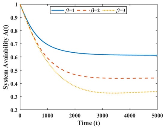
Figure 2. The repair time is $A\left(t\right)$ and falls in a gamma distribution for different $\beta$.

In the following, we assume $\beta =1$ (i.e., the repair time of the system is exponentially distributed) and continue to discuss the influence of different ${\lambda }_{c0}$ and ${\lambda }_{h0}$ on the instantaneous availability of the system.

Figure 3a,b show that $A\left(t\right)$ decreases with increases in ${\lambda }_{c0}$ and ${\lambda }_{h0}$. In addition, as time goes to infinity, the instantaneous availability of the system converges to a certain value.

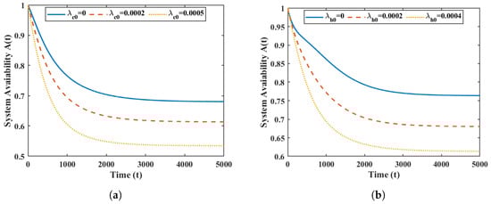
Figure 3. Effect of parameters ${\lambda }_{c0}$ and ${\lambda }_{h0}$ on $A\left(t\right)$. $\left(\mathbf{a}\right)$$A\left(t\right)$ for different ${\lambda }_{c0}$; $\left(\mathbf{b}\right)$$A\left(t\right)$ for different ${\lambda }_{h0}$.

Figure 4 reveals the effect of different ${\mu }_4$ on the instantaneous availability of the system. It is not difficult to find that $A\left(t\right)$ increases with increased ${\mu }_4$.

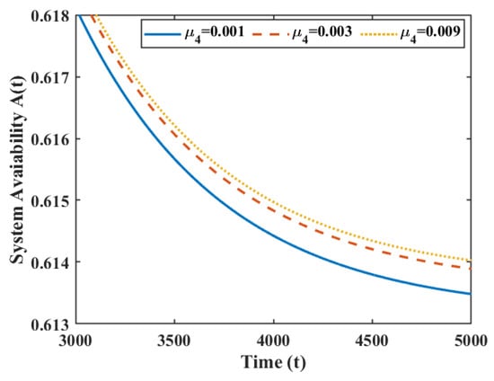
Figure 4. The repair time is $A\left(t\right)$ for an exponential distribution for different ${\mu }_4$.

Figure 5 indicates the effect of ${\lambda }_{c0}$ and ${\lambda }_{h0}$ on the system reliability and mean time to failure ($MTTF$). We note that $R\left(t\right)$(Figure 5a) and $MTTF$ (Figure 5b) decrease as ${\lambda }_{c0}$ increases. Obviously, reliability vanishes as time goes to infinity.

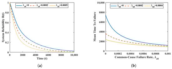
Figure 5. Reliability and $MTTF$ for exponentially distributed repair time. $\left(\mathbf{a}\right)$ Reliability for different ${\lambda }_{c0}$. $\left(\mathbf{b}\right)$ Effect of ${\lambda }_{h0}$ on MTTF.

Obviously, a similar conclusion can be drawn for the system’s failure frequency, $m_f\left(t\right)$, and the renewal frequency, $m_r\left(t\right)$. Therefore, it can be seen from the above figure and discussion that when the time tends to infinity, the instantaneous reliability index of the system tends to a constant value, which verifies the main results obtained in Section 5.

8. Conclusions

In this paper, we studied the dynamical solution problem of human–machine systems with human error and common-cause failure. We started from theory and used the theory of semigroups in functional analyses to model the system. The integral-differential equation was transformed into an abstract Cauchy problem in Banach space. Then, we proved the well-posedness of (9), studied the asymptotic behavior of its time-dependent solution, and showed that the time-dependent solution converges exponentially to its steady-state solution, obtaining asymptotic expressions for the time-dependent solution. In addition, the influence of each parameter on the system reliability were analyzed through concrete numerical examples. Therefore, engineers can design a more reliable, safe, and cost-effective system by using the results obtained in this paper. To a certain extent, it provides a theoretical basis for system reliability management and optimal scheduling.

If we know the spectral distribution of $\mathcal{H}+\mathcal{M}+\mathcal{S}$ in $\{\eta \in \mathbb{C}\mid \Re \eta \le -min\{\underline{{\mu }_{\varrho }},\underline{{\mu }_{\varrho +1}},$

and $\underline{{\mu }_{\varrho +2}}\left\}\right\}$, we may directly estimate $B,\omega$ in Theorem 7, which is important for engineers. Based on our knowledge of this subject, we believe $\mathcal{H}+\mathcal{M}+\mathcal{S}$ has a continuous spectrum in $\{\eta \in \mathbb{C}\mid \Re \eta \le -min\{\underline{{\mu }_{\varrho }},\underline{{\mu }_{\varrho +1}},\underline{{\mu }_{\varrho +2}}\}\}$. However, it is necessary to verify this and investigate more results.

References

- Cox, D.R. The analysis of non-Markovian stochastic processes by the inclusion of supplementary variables. Math. Proc. Camb. Philos. Soc. 1955, 51, 433–441. [Google Scholar] [CrossRef]
- Gaver, D.P. Time to failure and availability of parallel redundant systems with repair. IEEE Trans. Reliab. 1963, 12, 30–38. [Google Scholar] [CrossRef]
- Abbas, B.S.; Kuo, W. Stochastic effectiveness models for human-machine systems. IEEE Trans. Syst. Man Cybern. 1990, 20, 826–834. [Google Scholar] [CrossRef]
- Yang, N.F.; Dhillon, B.S. Stochastic analysis of a general standby system with constant human error and arbitrary system repair rates. Microelectron. Reliab. 1995, 35, 1037–1045. [Google Scholar] [CrossRef]
- Sridharan, V.; Mohanavadivu, P. Some statistical characteristics of a repairable, standby, human and machine system. IEEE Trans. Reliab. 1998, 47, 431–435. [Google Scholar] [CrossRef]
- Asadzadeh, S.M.; Azadeh, A. An integrated systemic model for optimization of condition-based maintenance with human error. Reliab. Eng. Syst. Saf. 2014, 124, 117–131. [Google Scholar] [CrossRef]
- Wang, J.; Xie, N.; Yang, N. Reliability analysis of a two-dissimilar-unit warm standby repairable system with priority in use. Commun. Stat. Theory Methods 2021, 50, 792–814. [Google Scholar] [CrossRef]
- Gupur, G. Well-posedness of the model describing a repairable, standby human & machine system. J. Syst. Sci. Complex. 2003, 16, 483–493. [Google Scholar]
- Gupur, G. Asymptotic property of the solution of a repairable, standby, human and machine system. Int. J. Pure Appl. Math. 2006, 8, 35–54. [Google Scholar]
- Aili, M.; Gupur, G. Further results on a repairable, standby, human and machine system. Int. J. Pure Appl. Math. 2015, 101, 571–594. [Google Scholar]
- Guo, W.H.; Wu, S.L. The Asymptotic Stability of a Solution of a Repairable Standby Human-Machine System. Math. Pract. Theory 2004, 10, 104–109. (In Chinese) [Google Scholar]
- Wang, W.L.; Xu, G.Q. The well-posedness and stability of a repairable standby human-machine system. Math. Comput. Model. 2006, 44, 1044–1052. [Google Scholar] [CrossRef]
- Narmada, S.; Jacob, M. Reliability analysis of a complex system with a deteriorating standby unit under common-cause failure and critical human error. Microelectron. Reliab. 1996, 36, 1287–1290. [Google Scholar] [CrossRef]
- Hajeeh, M.A. Availability of deteriorated system with inspection subject to common-cause failure and human error. Int. J. Oper. Res. 2011, 12, 207–222. [Google Scholar] [CrossRef]
- Liu, Z.; Liu, Y.; Cai, B. Dynamic Bayesian network modeling of reliability of subsea blowout preventer stack in presence of common cause failures. J. Loss Prev. Process Ind. 2015, 38, 58–66. [Google Scholar] [CrossRef]
- Shneiderman, B. Human-centered artificial intelligence: Reliable, safe & trustworthy. Int. J. Hum.–Comput. Interact. 2020, 36, 495–504. [Google Scholar]
- Xu, H.; Guo, W.; Guo, L. Stability of a General Repairable Human-Machine System. In Proceedings of the 2008 IEEE International Conference on Industrial Engineering and Engineering Management, Singapore, 8–11 December 2008; pp. 512–515. [Google Scholar]
- Fattorini, H.O. The Cauchy Problem; Cambridge University Press: Cambridge, UK, 1984. [Google Scholar]
- Gupur, G. Functional Analysis Methods for Reliability Models; Springer Science & Business Media: Berlin/Heidelberg, Germany, 2011. [Google Scholar]
- Nagel, R. One-Parameter Semigroups of Positive Operators; Springer: Berlin/Heidelberg, Germany, 1986. [Google Scholar]
- Engel, K.J.; Nagel, R. One-Parameter Semigroups for Linear Evolution Equations; Springer: New York, NY, USA, 2000. [Google Scholar]
- Gupur, G. On the asymptotic expression of the time-dependent solution of an M/G/1 queueing model. Partial Differ. Equ. Appl. 2022, 3, 21. [Google Scholar] [CrossRef]
Disclaimer/Publisher’s Note: The statements, opinions and data contained in all publications are solely those of the individual author(s) and contributor(s) and not of MDPI and/or the editor(s). MDPI and/or the editor(s) disclaim responsibility for any injury to people or property resulting from any ideas, methods, instructions or products referred to in the content. |
© 2023 by the authors. Licensee MDPI, Basel, Switzerland. This article is an open access article distributed under the terms and conditions of the Creative Commons Attribution (CC BY) license (https://creativecommons.org/licenses/by/4.0/).