Study on Dynamic Behavior of a Stochastic Predator–Prey System with Beddington–DeAngelis Functional Response and Regime Switching

Abstract

In this paper, by introducing environmental white noise and telegraph noise, we proposed a stochastic predator–prey model with the Beddington–DeAngelis type functional response and investigated its dynamical behavior. Persistence and extinction are two core contents of population model research, so we analyzed these two properties. The sufficient conditions of the strong persistence in the mean and extinction were established and the threshold between them was obtained. Moreover, we took stability into account and, by means of structuring a suitable Lyapunov function with regime switching, we proved that the stochastic system has a unique stationary distribution. Finally, numerical simulations were used to illustrate our theoretical results.

1. Introduction

Predator–prey models arise naturally in mathematical ecology, physics, and so on [1,2]. Beddington [3] and DeAngelis et al. [4] first introduced the Beddington–DeAngelis (B-D) type predator–prey model; we also refer the reader to [5,6,7,8]. In the literature, many scholars have focused on the following predator–prey system with the B-D functional response:

$$\left\{\begin{array}{cc}\hfill & \dot{x}\left(t\right)=x\left(t\right)[b_1-a_{11}x\left(t\right)-\frac{a_{12}y\left(t\right)}{1+\beta x\left(t\right)+\gamma y\left(t\right)}],\hfill \\ \hfill & \dot{y}\left(t\right)=y\left(t\right)[-b_2+\frac{a_{21}x\left(t\right)}{1+\beta x\left(t\right)+\gamma y\left(t\right)}],\hfill \end{array}\right.$$

(1)

where $x\left(t\right)$ and $y\left(t\right)$ represent predator and prey densities, respectively, and $b_i,a_{ij},\beta$ and $\gamma$ are positive constants, $i,j=1,2$; see [9,10,11,12,13,14,15,16,17,18,19,20,21] and the references therein. In [9], the authors studied the dynamics of a non-autonomous predator–prey system with the Beddington–DeAngelis functional response, and in [10,11], the authors established sufficient conditions for the existence of an almost periodic solution and a positive periodic solution of the non-autonomous B-D predator–prey system. The authors of [21] proposed the following stochastic B-D predator–prey system and the predator and prey in it are density dependent,

$$\left\{\begin{array}{cc}\hfill & dx\left(t\right)=x\left(t\right)[b_1-a_{11}x\left(t\right)-\frac{c_{1}y\left(t\right)}{m_1+m_{2}x\left(t\right)+m_{3}y\left(t\right)}]dt+\alpha x\left(t\right)d{B}_1\left(t\right),\hfill \\ \hfill & dy\left(t\right)=y\left(t\right)[-b_2+a_{22}y\left(t\right)+\frac{c_{2}x\left(t\right)}{m_1+m_{2}x\left(t\right)+m_{3}y\left(t\right)}]dt-\beta y\left(t\right)d{B}_2\left(t\right),\hfill \end{array}\right.$$

(2)

and they obtained the existence of the stationary distribution. The authors of [22] investigated the non-autonomous form of system (2) and discussed the moment boundedness and the growth rate of the population.

However, living things in nature are always more or less affected by environmental noise, the most important being white noise and colored noise (or telegraph noise); see [21,22,23,24,25,26,27,28,29,30,31,32,33,34] for more details. So far, the tools that can deal with stochastic models having colored noise (see [26,27,35,36,37,38,39,40]) are limited. Refs. [37,38] gave the methods for studying the ergodicity and stationary distribution of stochastic differential equations with Markovian switching and, based on them, the authors of [35,36,39] obtained the ergodic property for a Lotka–Volterra predator–prey model with white and colored noise and a Lotka–Volterra mutualistic system, respectively. Until recently, there is little research on the dynamical properties of a stochastic predator–prey model with the B-D functional response with regime switching. Therefore, in this work, we introduced white noise, which affects the intrinsic growth rate and death rate, that is, $b_1\to b_1+{\sigma }_1{\dot{B}}_1\left(t\right)$, $-b_2\to -b_2+{\sigma }_2{\dot{B}}_2\left(t\right)$ (${\sigma }_1^2$ and ${\sigma }_2^2$ represent the white noise intensities), and the continuous-time Markov chain ${\left\{r\left(t\right)\right\}}_{t\ge 0}$ taking values in a finite state space $\mathbb{S}=\{1,\dots ,N\}$ into system (1); then, it can be rewritten in the form:

$$\left\{\begin{array}{c}dx\left(t\right)=x\left(t\right)[b_1\left(r\left(t\right)\right)-a_{11}\left(r\left(t\right)\right)x\left(t\right)-\frac{a_{12}\left(r\left(t\right)\right)y\left(t\right)}{1+\beta x\left(t\right)+\gamma y\left(t\right)}]dt+{\sigma }_1\left(r\left(t\right)\right)x\left(t\right)d{B}_1\left(t\right),\hfill \\ dy\left(t\right)=y\left(t\right)[-b_2\left(r\left(t\right)\right)+\frac{a_{21}\left(r\left(t\right)\right)x\left(t\right)}{1+\beta x\left(t\right)+\gamma y\left(t\right)}]dt+{\sigma }_2\left(r\left(t\right)\right)y\left(t\right)d{B}_2\left(t\right).\hfill \end{array}\right.$$

(3)

In this model, $B_i\left(t\right)$ is 1-dimensional standard Brownian motion with $B_i\left(0\right)=0(i=1,2)$ defined on the complete probability space $(\mathsf{\Omega },\mathcal{F},{\left\{{\mathcal{F}}_t\right\}}_{t\ge 0},\mathbb{P})$ with a filtration ${\left\{{\mathcal{F}}_t\right\}}_{t\ge 0}$, satisfying the usual conditions (i.e., it is right continuous and ${\mathcal{F}}_0$ contains all P-null sets). Throughout this paper, we assume that, for each $k\in \mathbb{S}$, $b_i\left(k\right),a_{ij}\left(k\right)$, ${\sigma }_i\left(k\right)$, $\beta$, and $\gamma$ are positive constants, $i,j=1,2$.

We make the following arrangement for each chapter. Section 2 presents some basic theories. In Section 3, we discuss the strong persistence in the mean and the extinction. In Section 4, we establish the sufficient conditions for the stationary distribution. Section 5 proposes an example and figures to illustrate our results. This paper ends with our conclusions and plans for future research.

2. Preliminaries

We denote by $R_{+}^n$ the positive zone in $R^n$, i.e., $R_{+}^n=\{z\in R^n:z_i>0,1\le i\le n\}$. Define a Markov chain $r\left(t\right)$, which is right-continuous on the probability space $(\mathsf{\Omega },\mathcal{F},{\left\{{\mathcal{F}}_t\right\}}_{t\ge 0},\mathbb{P})$ taking values in a finite-state space $\mathbb{S}=\{1,\dots ,N\}$ and its generator $\mathrm{\Gamma }={\left(q_{ij}\right)}_{1\le i,j\le N}$ is

$$P\{r(t+\mathrm{\Delta }t)=j|r\left(t\right)=i\}=\left\{\begin{array}{c}\hfill q_{ij}\mathrm{\Delta }t+o\left(\mathrm{\Delta }t\right),\mathrm{if}i\ne j,\\ \hfill 1+q_{ii}\mathrm{\Delta }t+o\left(\mathrm{\Delta }t\right),\mathrm{if}i=j,\end{array}\right.$$

(4)

where $\mathrm{\Delta }t>0$, $q_{ij}$ is the transition probability from the state i to state j and $q_{ij}\ge 0$ ($i\ne j$), while $q_{ii}=-{\sum }_{i\ne j}{q}_{ij}.$ In this paper, we assumed that $q_{ij}>0$ if $i\ne j$ and the Markov chain $r\left(t\right)$ is irreducible and independent of the Brownian motion. In light of the theory of a Markov chain, the finite states imply the ergodic property and positive recurrence of $r\left(t\right),t\ge 0$. Hence, the Markov chain has a unique stationary distribution $\pi =({\pi }_1,\dots ,{\pi }_N)\in R^{1\times N}$ such that $\pi \mathrm{\Gamma }=0$, ${\mathrm{\Sigma }}_{k=1}^N{\pi }_k=1$, ${\pi }_k>0,\forall k\in \mathbb{S}$ and, for any vector $\overrightarrow{c}={(c\left(1\right),\dots ,c\left(N\right))}^T$,

$$\underset{t\to \infty }{lim}\frac{1}{t}{\int }_0^{t}c\left(r\left(s\right)\right)ds=\sum _{k\in \mathbb{S}}{\pi }_{k}c\left(k\right).$$

Let $\widehat{c}={min}_{k\in \mathbb{S}}\left\{c\left(k\right)\right\}$, $\check{c}={max}_{k\in \mathbb{S}}\left\{c\left(k\right)\right\}$ and

$$\frac{1}{t}{\int }_0^{t}f\left(s\right)ds=⟨f\left(t\right)⟩.$$

To investigate the positive recurrence and the ergodic property of the stochastic system (3), we first introduced the following lemma (see [37,38]). Let $\left(\varphi \right(t),r(t\left)\right)$ be the diffusion process of the equation:

$$\left\{\begin{array}{c}d\varphi \left(t\right)=f\left(\varphi \right(t),r(t\left)\right)dt+g\left(\varphi \right(t),r(t\left)\right)dB\left(t\right),\\ \varphi \left(0\right)=\varphi ,r\left(0\right)=r,\end{array}\right.$$

(5)

where $B(·)$ and $r(·)$ are the d-dimensional Brownian motion and the right-continuous Markov chain, respectively, and $f(·,·):R^n\times \mathbb{S}\to R^n$, $g(·,·):R^n\times \mathbb{S}\to R^{n\times d}$ with $g(\varphi ,k)g^T(\varphi ,k)=\mathcal{C}(\varphi ,k)$. For any twice continuously differentiable function $V(·,k)$, for each $k\in \mathbb{S}$, define the differential operator $\mathcal{L}$ by

$$\mathcal{L}V(\varphi ,·)\left(k\right)=\sum _{i=1}^n{f}_i(\varphi ,k)\frac{\partial V(\varphi ,k)}{\partial {\varphi }_i}+\frac{1}{2}\sum _{i,j=1}^n{\mathcal{C}}_{ij}(\varphi ,k)\frac{{\partial }^{2}V(\varphi ,k)}{\partial {\varphi }_i\partial {\varphi }_j}+\mathrm{\Gamma }V(\varphi ,·)\left(k\right),$$

where

$$\mathrm{\Gamma }V(\varphi ,·)\left(k\right)=\sum _{u\ne k,u\in \mathbb{S}}{\gamma }_{ku}(V(\varphi ,u)-V(\varphi ,k)),k\in \mathbb{S}.$$

Lemma 1.

Suppose the following conditions hold:

(i) 

For $i\ne j,q_{ij}>0;$

(ii) 

For each $k\in \mathbb{S},\mathcal{C}(\varphi ,k)$ is symmetric and satisfies ${\kappa }_0{\left|\xi \right|}^2\le {\xi }^T\mathcal{C}(\varphi ,k)\xi \le {\kappa }_0^{-1}{\left|\xi \right|}^2$ for all $\xi \in R^n$, with some constant ${\kappa }_0\in (0,1]$ for all $\varphi \in R^n;$

(iii) 

There exists a nonnegative $C^2$-function $V(·,k)$ such that $\mathcal{L}V(\varphi ,k)\le -1$ outside some compact set.

Then, $\left(\varphi \right(t),r(t\left)\right)$ of the system (5) is ergodic and positive recurrent, and then there exists a unique stationary density $\mu (·,·)$ and, for any Borel measurable function $f(·,·):R^n\times \mathbb{S}\to R$ such that

$$\sum _{k\in \mathbb{S}}{\int }_{R^n}\left|f(\varphi ,k)\right|\mu (\varphi ,k)d\varphi <\infty ,$$

we have

$$\mathbb{P}(\frac{1}{t}{\int }_0^{t}f(\varphi \left(s\right),r\left(s\right))ds\to \sum _{k\in \mathbb{S}}{\int }_{R^n}f(\varphi ,k)\mu (\varphi ,k)d\varphi \to \infty )=1a.s.$$

Lemma 2.

Let $\varphi \left(t\right)\in C[\mathsf{\Omega }\times [0,+\infty ),R_{+}]$. If, for any $t\ge T$, there exists positive constants ${\kappa }_0,T$, $\kappa \ge 0$ and ${\beta }_i$, $1\le i\le n,$ such that

$$log\varphi \left(t\right)\ge \kappa t-{\kappa }_0{\int }_0^t\varphi \left(s\right)ds+\sum _{i=1}^n{\beta }_i{B}_i\left(t\right),$$

then

$$\underset{t\to \infty }{lim\; inf}\frac{1}{t}{\int }_0^t\varphi \left(s\right)ds\ge \frac{\kappa }{{\kappa }_0},a.s.$$

Lemma 3.

For any given initial value $(x\left(0\right),y\left(0\right),r\left(0\right))\in R_{+}^2\times \mathbb{S}$, system (3) has a unique continuous positive solution which will remain in $R_{+}^2\times \mathbb{S}$ with probability 1.

The proof of Lemma 3 is standard [27,28,41,42], so we only list the key point, namely the construction of the Lyapunov function,

$$V(x,y)=x-1-lnx+y-1-lny.$$

3. The Strong Persistence in the Mean and the Extinction

In this section, we will demonstrate two critical aspects of population dynamics. Before the proof, we first review the basic concepts which can be found in the article [28].

Definition 1.

⋄

$System\left(3\right)isextinctivealmostsurely(a.s.),if{\displaystyle \underset{t\to \infty }{lim}}y\left(t\right)=0a.s.;$

⋄

$System\left(3\right)isstronglypersistentinthemean,if{\displaystyle \underset{t\to \infty }{lim\; inf}}⟨y\left(t\right)⟩>0a.s..$

Let $X\left(t\right)$ be a homogeneous Markov process, which is exactly depicted by the following SDE system:

$$dX\left(t\right)=X\left(t\right)[b_1\left(r\left(t\right)\right)-a_{11}\left(r\left(t\right)\right)X\left(t\right)]dt+{\sigma }_1\left(r\left(t\right)\right)X\left(t\right)d{B}_1\left(t\right).$$

(6)

$x\left(0\right)=X\left(0\right)>0$. The properties of the 1-dimensional stochastic system (6) are listed as follows:

(a)

${lim}_{t\to \infty }X\left(t\right)=0$ a.s., if the condition ${\sum }_{k\in \mathbb{S}}{\pi }_k[a\left(k\right)-\frac{{\sigma }_1^2\left(k\right)}{2}]<0$ holds (see [26]);

(b)

${lim}_{t\to \infty }\frac{M_1\left(t\right)}{t}=0a.s.,$ by the strong law of large numbers for martingales (see [35], p. 16), where $M_1\left(t\right)={\int }_0^t{\sigma }_1\left(r\left(s\right)\right)d{B}_1\left(s\right)$ is a real-valued continuous local martingale;

(c)

${lim}_{t\to \infty }\frac{logX\left(t\right)}{t}=0$ (see Theorem 5.1 in [43]);

(d)

According to the literature [44], if ${\sum }_{k\in \mathbb{S}}{\pi }_k[a\left(k\right)-\frac{{\sigma }_1^2\left(k\right)}{2}]>0$, for any Borel measurable function $g(·,·):R\times \mathbb{S}\to R$, then SDE (6) has a unique stationary distribution $\nu (·,·)$ with the ergodic property:

$$\underset{t\to \infty }{lim}\frac{1}{t}{\int }_0^{t}g(X\left(s\right),r\left(s\right))ds=\sum _{k\in \mathbb{S}}{\int }_{R_{+}}g(x,k)\nu (dx,k)a.s.$$

On the basis of the well-known comparison theorem and $\left(\mathbf{a}\right)$, for any $t\ge 0$, $x\left(t\right)\le X\left(t\right)$ and ${lim}_{t\to \infty }X\left(t\right)=0$ a.s., which can lead to ${lim}_{t\to \infty }x\left(t\right)=0$ a.s., and then ${lim}_{t\to \infty }y\left(t\right)=0$ a.s. In this paper, we suppose that ${\sum }_{k\in \mathbb{S}}{\pi }_k[b_1\left(k\right)-\frac{{\sigma }_1^2\left(k\right)}{2}]>0$, in order to prevent the extinction of the predator caused by the prey’s extinction.

Furthermore, the generalized It$\widehat{o}$’s formula on system (6) shows that

$$\frac{logX\left(t\right)-logX\left(0\right)}{t}=⟨b_1\left(r\left(t\right)\right)-\frac{{\sigma }_1^2\left(r\left(t\right)\right)}{2}⟩-⟨a_{11}\left(r\left(t\right)\right)X\left(t\right)⟩+\frac{M_1\left(t\right)}{t}.$$

(7)

From $\left(\mathbf{b}\right)$, $\left(\mathbf{c}\right)$ and $\left(\mathbf{d}\right)$, we have, respectively, ${lim}_{t\to \infty }\frac{M_1\left(t\right)}{t}=0a.s.,$${lim}_{t\to \infty }\frac{logX\left(t\right)}{t}=0$ and

$$\underset{t\to \infty }{lim}⟨a_{11}\left(r\left(t\right)\right)X\left(t\right)⟩=\sum _{k\in \mathbb{S}}{a}_{11}\left(k\right){\int }_{R_{+}}x\nu (dx,k)a.s.,$$

which follows from (7) that

$$\sum _{k\in \mathbb{S}}{a}_{11}\left(k\right){\int }_{R_{+}}x\nu (dx,k)=\sum _{k\in \mathbb{S}}{\pi }_k[b_1\left(k\right)-\frac{{\sigma }_1^2\left(k\right)}{2}]a.s.$$

(8)

The equality (8) will play a crucial role in the following theorem about the properties of population dynamics.

Theorem 1.

In system (3), for any given initial value $(x\left(0\right),y\left(0\right),r\left(0\right))\in R_{+}^2\times \mathbb{S}$, if ${\sum }_{k\in \mathbb{S}}{\pi }_k$$[b_1\left(k\right)-\frac{{\sigma }_1^2\left(k\right)}{2}]>0$, then the following statements hold:

(i) 

If $\kappa <0$, the predator population goes to extinction a.s.;

(ii) 

If $\kappa >0$, system (3) will be strongly persistent in the mean.

Here,

$$\kappa =\sum _{k\in \mathbb{S}}{\int }_{R_{+}}\frac{a_{21}\left(k\right)x}{1+\beta x}\nu (dx,k)-\sum _{k\in \mathbb{S}}{\pi }_k[b_2\left(k\right)+\frac{{\sigma }_2^2\left(k\right)}{2}].$$

Proof. 

(i)

On the second equation of (3), we use the generalized It$\widehat{o}$’s formula and then

$$\begin{array}{cc}\hfill \frac{logy\left(t\right)-logy\left(0\right)}{t}=& -⟨b_2\left(r\left(t\right)\right)+\frac{{\sigma }_2^2\left(r\left(t\right)\right)}{2}⟩+⟨\frac{a_{21}\left(r\left(t\right)\right)x\left(t\right)}{1+\beta x\left(t\right)+\gamma y\left(t\right)}⟩+\frac{M_2\left(t\right)}{t}\hfill \\ \hfill & \le -⟨b_2\left(r\left(t\right)\right)+\frac{{\sigma }_2^2\left(r\left(t\right)\right)}{2}⟩+⟨\frac{a_{21}\left(r\left(t\right)\right)X\left(t\right)}{1+\beta X\left(t\right)}⟩+\frac{M_2\left(t\right)}{t},\hfill \end{array}$$

(9)

where $M_2\left(t\right)={\int }_0^t{\sigma }_2\left(r\left(s\right)\right)d{B}_2\left(s\right)$ is a martingale. From (7) and (8) we have

$$\underset{t\to \infty }{lim\; sup}\frac{logy\left(t\right)}{t}\le \sum _{k\in \mathbb{S}}{\int }_{R_{+}}\frac{a_{21}\left(k\right)x}{1+\beta x}\nu (dx,k)-\sum _{k\in \mathbb{S}}{\pi }_k[b_2\left(k\right)+\frac{{\sigma }_2^2\left(k\right)}{2}]=\kappa a.s.$$

(10)

If $\kappa <0$, then $y\left(t\right)$ tends to zero a.s., so $\left(i\right)$ holds.

(ii)

Applying It$\widehat{o}$’s formula on the first equation of (3) gives

$$\begin{array}{c}\hfill \frac{logx\left(t\right)-logx\left(0\right)}{t}=⟨b_1\left(r\left(t\right)\right)-\frac{{\sigma }_1^2\left(r\left(t\right)\right)}{2}⟩-⟨a_{11}\left(r\left(t\right)\right)x\left(t\right)⟩-⟨\frac{a_{12}\left(r\left(t\right)\right)y\left(t\right)}{1+\beta x\left(t\right)+\gamma y\left(t\right)}⟩+\frac{M_1\left(t\right)}{t}.\end{array}$$

(11)

From (7) and (11), we have

$$\begin{array}{cc}\hfill 0\ge \frac{logx\left(t\right)-logX\left(t\right)}{t}& =⟨a_{11}\left(r\left(t\right)\right)[X\left(t\right)-x\left(t\right)]⟩-⟨\frac{a_{12}\left(r\left(t\right)\right)y\left(t\right)}{1+\beta x\left(t\right)+\gamma y\left(t\right)}⟩\ge {\widehat{a}}_{11}⟨X\left(t\right)-x\left(t\right)⟩-{\check{a}}_{12}⟨y\left(t\right)⟩,\hfill \end{array}$$

and so

$$⟨X\left(t\right)-x\left(t\right)⟩\le \frac{{\check{a}}_{12}}{{\widehat{a}}_{11}}⟨y\left(t\right)⟩.$$

(12)

Substituting (12) into (9) yields

$$\begin{array}{cc}\hfill & \frac{logy\left(t\right)-logy\left(0\right)}{t}\hfill \\ \hfill & =-⟨b_2\left(r\left(t\right)\right)+\frac{{\sigma }_2^2\left(r\left(t\right)\right)}{2}⟩+⟨\frac{a_{21}\left(r\left(t\right)\right)x\left(t\right)}{1+\beta x\left(t\right)+\gamma y\left(t\right)}⟩+\frac{M_2\left(t\right)}{t}\hfill \\ \hfill & =-⟨b_2\left(r\left(t\right)\right)+\frac{{\sigma }_2^2\left(r\left(t\right)\right)}{2}⟩+⟨\frac{a_{21}\left(r\left(t\right)\right)X\left(t\right)}{1+\beta X\left(t\right)}⟩-⟨\frac{a_{21}\left(r\left(t\right)\right)X\left(t\right)}{1+\beta X\left(t\right)}-\frac{a_{21}\left(r\left(t\right)\right)x\left(t\right)}{1+\beta x\left(t\right)+\gamma y\left(t\right)}⟩+\frac{M_2\left(t\right)}{t}\hfill \\ \hfill & =-⟨b_2\left(r\left(t\right)\right)+\frac{{\sigma }_2^2\left(r\left(t\right)\right)}{2}⟩+⟨\frac{a_{21}\left(r\left(t\right)\right)X\left(t\right)}{1+\beta X\left(t\right)}⟩\hfill \\ \hfill & -⟨\frac{a_{21}\left(r\left(t\right)\right)[X\left(t\right)(1+\beta x\left(t\right)+\gamma y\left(t\right))-x\left(t\right)(1+\beta X\left(t\right))]}{(1+\beta X(t\left)\right)(1+\beta x(t)+\gamma y(t\left)\right)}⟩+\frac{M_2\left(t\right)}{t}\hfill \\ \hfill & =-⟨b_2\left(r\left(t\right)\right)+\frac{{\sigma }_2^2\left(r\left(t\right)\right)}{2}⟩+⟨\frac{a_{21}\left(r\left(t\right)\right)X\left(t\right)}{1+\beta X\left(t\right)}⟩\hfill \\ \hfill & -⟨\frac{a_{21}\left(r\left(t\right)\right)[X\left(t\right)-x\left(t\right)](1+\gamma y\left(t\right))}{(1+\beta X(t\left)\right)(1+\beta x(t)+\gamma y(t\left)\right)}+\frac{a_{21}\left(r\left(t\right)\right)\gamma x\left(t\right)y\left(t\right)}{(1+\beta X(t\left)\right)(1+\beta x(t)+\gamma y(t\left)\right)}⟩+\frac{M_2\left(t\right)}{t}\hfill \\ \hfill & \ge -⟨b_2\left(r\left(t\right)\right)+\frac{{\sigma }_2^2\left(r\left(t\right)\right)}{2}⟩+⟨\frac{a_{21}\left(r\left(t\right)\right)X\left(t\right)}{1+\beta X\left(t\right)}⟩-{\check{a}}_{21}⟨X\left(t\right)-x\left(t\right)⟩-\frac{\gamma {\check{a}}_{21}}{\beta }⟨y\left(t\right)⟩+\frac{M_2\left(t\right)}{t}\hfill \\ \hfill & \ge -⟨b_2\left(r\left(t\right)\right)+\frac{{\sigma }_2^2\left(r\left(t\right)\right)}{2}⟩+⟨\frac{a_{21}\left(r\left(t\right)\right)X\left(t\right)}{1+\beta X\left(t\right)}⟩-{\check{a}}_{21}(\frac{{\check{a}}_{12}}{{\widehat{a}}_{11}}+\frac{\gamma }{\beta })⟨y\left(t\right)⟩+\frac{M_2\left(t\right)}{t}.\hfill \end{array}$$

(13)

Here,

$$\underset{t\to \infty }{lim}\frac{M_2\left(t\right)}{t}=0a.s.$$

The property of inferior limits implies that, for arbitrary $\epsilon >0$, there exists $t>0$ such that

$$-⟨b_2\left(r\left(t\right)\right)+\frac{{\sigma }_2^2\left(r\left(t\right)\right)}{2}⟩+⟨\frac{a_{21}\left(r\left(t\right)\right)X\left(t\right)}{1+\beta X\left(t\right)}⟩\ge \sum _{k\in \mathbb{S}}{\int }_{R_{+}}\frac{a_{21}\left(k\right)x}{1+\beta x}\nu (dx,k)-\sum _{k\in \mathbb{S}}{\pi }_k[b_2\left(k\right)+\frac{{\sigma }_2^2\left(k\right)}{2}]-\frac{\epsilon }{2}=\kappa -\frac{\epsilon }{2}$$

and $\frac{M_2\left(t\right)}{t}\ge -\frac{\epsilon }{2}$. Making use of these inequalities, one can obtain from (13) that

$$\frac{logy\left(t\right)-logy\left(0\right)}{t}\ge \kappa -\epsilon -{\check{a}}_{21}(\frac{{\check{a}}_{12}}{{\widehat{a}}_{11}}+\frac{\gamma }{\beta })⟨y\left(t\right)⟩,$$

(14)

and from the arbitrariness of $\epsilon$ and Lemma 2, it is easy to deduce

$$\underset{t\to \infty }{lim\; inf}⟨y\left(t\right)⟩\ge \frac{\kappa }{{\check{a}}_{21}(\frac{{\check{a}}_{12}}{{\widehat{a}}_{11}}+\frac{\gamma }{\beta })}>0a.s.$$

(15)

Thus, $\left(ii\right)$ holds and, furthermore, the threshold $\kappa$ between the strong persistence in the mean and the extinction of the SDE (3) is obtained. A physical interpretation of the threshold $\kappa$ is that, when the capture density of predators exceeds the sum of fluctuation intensity and mortality, the predator population will persist for a long time. If not, it tends to become extinct. A more relevant physical analysis can be referred to in [41]. □

4. Ergodic Property of Positive Recurrence

The aim of this section is to prove the ergodic property and the existence of the unique stationary distribution of the solution in system (3). First, we utilize variable substitution $x\left(t\right)=e^{\xi \left(t\right)}$, $y\left(t\right)=e^{\eta \left(t\right)}$ and It$\widehat{o}$’s formula, which yield the following transformed system:

$$\left\{\begin{array}{c}\hfill d\xi \left(t\right)=(b_1\left(r\left(t\right)\right)-\frac{{\sigma }_1^2\left(r\left(t\right)\right)}{2}-a_{11}\left(r\left(t\right)\right)e^{\xi \left(t\right)}-\frac{a_{12}\left(r\left(t\right)\right)e^{\eta \left(t\right)}}{1+\beta e^{\xi \left(t\right)}+\gamma e^{\eta \left(t\right)}})dt+{\sigma }_1\left(r\left(t\right)\right)d{B}_1\left(t\right),\\ \hfill d\eta \left(t\right)=(-b_2\left(r\left(t\right)\right)-\frac{{\sigma }_2^2\left(r\left(t\right)\right)}{2}+\frac{a_{21}\left(r\left(t\right)\right)e^{\xi \left(t\right)}}{1+\beta e^{\xi \left(t\right)}+\gamma e^{\eta \left(t\right)}})dt+{\sigma }_2\left(r\left(t\right)\right)d{B}_2\left(t\right),\end{array}\right.$$

(16)

with the initial value $\left(\xi \right(0),\eta (0\left)\right)=(logx(0),logy(0\left)\right)$. Hence, our aim is equivalent to demonstrating them in system (16) (see [35]).

In what follows, let us introduce the assumption:

$$\begin{array}{c}\hfill \left(\mathbf{A}\right)\overline{\kappa }=\frac{{\widehat{a}}_{21}}{{\check{a}}_{11}+\beta {\widehat{b}}_1}\sum _{k\in \mathbb{S}}{\pi }_k[{\widehat{b}}_1-\frac{{\sigma }_1^2\left(k\right)}{2}]-\sum _{k\in \mathbb{S}}{\pi }_k[b_2\left(k\right)+\frac{{\sigma }_2^2\left(k\right)}{2}]>0.\end{array}$$

Theorem 2.

If assumption $\left(A\right)$ holds, then for any $k\in \mathbb{S}$ and for any given initial value $(x\left(0\right),y\left(0\right),r\left(0\right))\in R_{+}^2\times \mathbb{S}$, the solution of system (3) is ergodic and has a unique stationary distribution in $R_{+}^2\times \mathbb{S}$.

Proof. 

We will apply Lemma 1. For any sufficiently small number $0<ϵ<1$, define a bounded open subset

$$\mathcal{D}=\{(\xi ,\eta ):|\xi |<log{ϵ}^{-1},|\eta |<log{ϵ}^{-1},(\xi ,\eta )\in R^2\}.$$

Obviously, condition $\left(i\right)$ in Lemma 1 is satisfied by the assumption $q_{ij}>0,i\ne j$ in Section 2. Let $g(z,k)=diag({\sigma }_1\left(k\right),{\sigma }_2\left(k\right))(k\in \mathbb{S})$, and then $\mathcal{C}(z,k)=g(z,k)g^T(z,k)=diag({\sigma }_1^2\left(k\right),{\sigma }_2^2\left(k\right))$ is positive definite. Consequently, condition $\left(ii\right)$ in Lemma 1 holds. Now, we check condition $\left(iii\right)$ in Lemma 1.

Define a $C^2$-function $V:R^2\times \mathbb{S}\to R_{+}$ by

$$\begin{array}{cc}\hfill V(\xi ,\eta ,k)& =M(-\eta +\frac{{\widehat{a}}_{21}}{{\check{a}}_{11}+\beta {\widehat{b}}_1}[log(1+\beta e^{\xi })-\xi +\frac{{\check{a}}_{12}}{{\widehat{b}}_2}{e}^{\eta }\left]\right)+[e^{\xi }+p{e}^{\eta }]-\varphi ({\xi }_0,{\eta }_0)+M({\varpi }_k+\left|\varpi \right|)\hfill \\ \hfill & =V_1(\xi ,\eta )+V_2(\xi ,\eta )-\varphi ({\xi }_0,{\eta }_0)+V_3\left(k\right);\hfill \end{array}$$

(17)

here, $p=\frac{{\widehat{a}}_{12}}{{\check{a}}_{21}}$, $M=(2/\overline{\kappa })max\{2,{sup}_{(\xi ,\eta )\in R^2}\{-\frac{{\widehat{a}}_{11}}{2}{e}^{2\xi }-\frac{p{\widehat{b}}_2}{2}{e}^{\eta }+{\check{b}}_1{e}^{\xi }\}\}$ and, obviously, $\frac{M\overline{\kappa }}{4}\ge 1$. Here, $\varpi ={({\varpi }_1,\dots ,{\varpi }_N)}^T,\left|\varpi \right|=\sqrt{{\varpi }_1^2+\dots +{\varpi }_N^2}$, ${\varpi }_k(k\in \mathbb{S})$ will be determined in the proof. We put $\left|\varpi \right|$ in order to make ${\varpi }_k+\left|\varpi \right|$ non-negative. Here, $\varphi (\xi ,\eta )=V_1(\xi ,\eta )+V_2(\xi ,\eta )$. From the monotonically property of the partial derivative equations, it is easy to see that $\varphi (\xi ,\eta )$ has a unique minimum point $({\xi }_0,{\eta }_0)$ (a similar procedure is given in [39]). Hence, we assert that $\varphi (\xi ,\eta )-\varphi ({\xi }_0,{\eta }_0)\ge 0$, so $V(\xi ,\eta ,k)$ is non-negative.

Note,

$$\begin{array}{cc}\hfill \mathcal{L}(-\eta )& =b_2\left(k\right)+\frac{{\sigma }_2^2\left(k\right)}{2}-\frac{a_{21}\left(k\right)e^{\xi }}{1+\beta e^{\xi }+\gamma e^{\eta }}\hfill \\ \hfill & =b_2\left(k\right)+\frac{{\sigma }_2^2\left(k\right)}{2}-\frac{a_{21}\left(k\right)e^{\xi }}{1+\beta e^{\xi }}+(\frac{a_{21}\left(k\right)e^{\xi }}{1+\beta e^{\xi }}-\frac{a_{21}\left(k\right)e^{\xi }}{1+\beta e^{\xi }+\gamma e^{\eta }})\hfill \\ \hfill & \le b_2\left(k\right)+\frac{{\sigma }_2^2\left(k\right)}{2}-\frac{{\widehat{a}}_{21}{\widehat{b}}_1}{{\check{a}}_{11}+\beta {\widehat{b}}_1}+{\widehat{a}}_{21}(\frac{\frac{{\widehat{b}}_1}{{\check{a}}_{11}}}{1+\beta ·\frac{{\widehat{b}}_1}{{\check{a}}_{11}}}-\frac{e^{\xi }}{1+\beta e^{\xi }})+\frac{a_{21}\left(k\right)\gamma e^{\xi +\eta }}{(1+\beta e^{\xi })(1+\beta e^{\xi }+\gamma e^{\eta })}\hfill \\ \hfill & \le b_2\left(k\right)+\frac{{\sigma }_2^2\left(k\right)}{2}-\frac{{\widehat{a}}_{21}{\widehat{b}}_1}{{\check{a}}_{11}+\beta {\widehat{b}}_1}+\frac{{\widehat{a}}_{21}}{{\check{a}}_{11}+\beta {\widehat{b}}_1}·\frac{{\widehat{b}}_1-{\check{a}}_{11}{e}^{\xi }}{1+\beta e^{\xi }}+\frac{{\check{a}}_{21}\gamma e^{\xi +\eta }}{1+\beta e^{\xi }+\gamma e^{\eta }},\hfill \end{array}$$

(18)

and

$$\begin{array}{cc}\hfill & \mathcal{L}[log(1+\beta e^{\xi })-\xi +\frac{{\check{a}}_{12}}{{\widehat{b}}_2}{e}^{\eta }]\hfill \\ \hfill & =[\frac{\beta e^{\xi }(b_1\left(k\right)-a_{11}\left(k\right)e^{\xi })}{1+\beta e^{\xi }}-\frac{\beta a_{12}\left(k\right)e^{\xi +\eta }}{(1+\beta e^{\xi })(1+\beta e^{\xi }+\gamma e^{\eta })}-\frac{{\beta }^2{\sigma }_1^2\left(k\right)e^{2\xi }}{2{(1+\beta e^{\xi })}^2}]\hfill \\ \hfill & +[-b_1\left(k\right)+\frac{{\sigma }_1^2\left(k\right)}{2}+a_{11}\left(k\right)e^{\xi }+\frac{a_{12}\left(k\right)e^{\eta }}{1+\beta e^{\xi }+\gamma e^{\eta }}]+\frac{{\check{a}}_{12}}{{\widehat{b}}_2}[-b_2\left(k\right)e^{\eta }+\frac{a_{21}\left(k\right)e^{\xi +\eta }}{1+\beta e^{\xi }+\gamma e^{\eta }}]\hfill \\ \hfill & \le [b_1\left(k\right)-a_{11}\left(k\right)e^{\xi }-\frac{b_1\left(k\right)-a_{11}\left(k\right)e^{\xi }}{1+\beta e^{\xi }}]+[-b_1\left(k\right)+\frac{{\sigma }_1^2\left(k\right)}{2}+a_{11}\left(k\right)e^{\xi }+{\check{a}}_{12}{e}^{\eta }]\hfill \\ \hfill & +\frac{{\check{a}}_{12}}{{\widehat{b}}_2}[-{\widehat{b}}_2{e}^{\eta }+\frac{{\check{a}}_{21}{e}^{\xi +\eta }}{1+\beta e^{\xi }+\gamma e^{\eta }}]\hfill \\ \hfill & \le \frac{{\sigma }_1^2\left(k\right)}{2}-\frac{{\widehat{b}}_1-{\check{a}}_{11}{e}^{\xi }}{1+\beta e^{\xi }}+\frac{{\check{a}}_{12}{\check{a}}_{21}{e}^{\xi +\eta }}{{\widehat{b}}_2(1+\beta e^{\xi }+\gamma e^{\eta })}.\hfill \end{array}$$

(19)

Thus,

$$\begin{array}{c}\hfill \mathcal{L}{V}_1(\xi ,\eta )\le M(-\frac{{\widehat{a}}_{21}}{{\check{a}}_{11}+\beta {\widehat{b}}_1}[{\widehat{b}}_1-\frac{{\sigma }_1^2\left(k\right)}{2}]+[b_2\left(k\right)+\frac{{\sigma }_2^2\left(k\right)}{2}]+{\check{a}}_{21}[\frac{{\widehat{a}}_{21}{\check{a}}_{12}}{{\widehat{b}}_2({\check{a}}_{11}+\beta {\widehat{b}}_1)}+\gamma ]\frac{e^{\xi +\eta }}{1+\beta e^{\xi }+\gamma e^{\eta }}).\end{array}$$

(20)

Next, for any $k\in \mathbb{S}$,

$$\mathcal{L}{V}_3\left(k\right)=M\sum _{l\ne k,l\in \mathbb{S}}{\gamma }_{kl}({\varpi }_l-{\varpi }_k).$$

(21)

Define a vector $\kappa ={({\kappa }_1,\dots ,{\kappa }_N)}^T$ with ${\kappa }_k=\frac{{\widehat{a}}_{21}}{{\check{a}}_{11}+\beta {\widehat{b}}_1}[{\widehat{b}}_1-\frac{{\sigma }_1^2\left(k\right)}{2}]-[b_2\left(k\right)+\frac{{\sigma }_2^2\left(k\right)}{2}]$. Note that the generator matrix $\mathrm{\Gamma }$ is irreducible, then for ${\kappa }_k$, there exists a solution of the poisson system expressed as $\varpi ={({\varpi }_1,\dots ,{\varpi }_N)}^T$ (see Lemma 2.3 in [44]), such that

$$\mathrm{\Gamma }\varpi -\kappa =-\left(\sum _{j=1}^N{\pi }_j{\kappa }_j\right)\overrightarrow{1},$$

(22)

where $\overrightarrow{1}$ denotes the column vector with all its entries equal to 1. Hence, for all $k\in \mathbb{S}$, we have that

$$\begin{array}{cc}\hfill & \sum _{l\ne k,l\in \mathbb{S}}{\gamma }_{kl}({\varpi }_l-{\varpi }_k)-(\frac{{\widehat{a}}_{21}}{{\check{a}}_{11}+\beta {\widehat{b}}_1}[{\widehat{b}}_1-\frac{{\sigma }_1^2\left(k\right)}{2}]-[b_2\left(k\right)+\frac{{\sigma }_2^2\left(k\right)}{2}])\hfill \\ \hfill & =-(\frac{{\widehat{a}}_{21}}{{\check{a}}_{11}+\beta {\widehat{b}}_1}\sum _{k\in \mathbb{S}}{\pi }_k[{\widehat{b}}_1-\frac{{\sigma }_1^2\left(k\right)}{2}]-\sum _{k\in \mathbb{S}}{\pi }_k[b_2\left(k\right)+\frac{{\sigma }_2^2\left(k\right)}{2}])\hfill \\ \hfill & =-\overline{\kappa }.\hfill \end{array}$$

(23)

Combining (20), (21), and (23), yields $\mathcal{L}(V_1+V_3)\le M(-\overline{\kappa }+{\check{a}}_{21}[\frac{{\widehat{a}}_{21}{\check{a}}_{12}}{{\widehat{b}}_2({\check{a}}_{11}+\beta {\widehat{b}}_1)}+\gamma ]\frac{e^{\xi +\eta }}{1+\beta e^{\xi }+\gamma e^{\eta }}).$ Additionally,

$$\begin{array}{cc}\hfill \mathcal{L}{V}_2(\xi ,\eta )& =b_1\left(k\right)e^{\xi }-a_{11}\left(k\right)e^{2\xi }-\frac{a_{12}\left(k\right)e^{\xi +\eta }}{1+\beta e^{\xi }+\gamma e^{\eta }}-p{b}_2\left(k\right)e^{\eta }+\frac{p{a}_{21}\left(k\right)e^{\xi +\eta }}{1+\beta e^{\xi }+\gamma e^{\eta }}\hfill \\ \hfill & \le {\check{b}}_1{e}^{\xi }-{\widehat{a}}_{11}{e}^{2\xi }-p{\widehat{b}}_2{e}^{\eta }-\frac{{\widehat{a}}_{12}{e}^{\xi +\eta }}{1+\beta e^{\xi }+\gamma e^{\eta }}+\frac{p{\check{a}}_{21}{e}^{\xi +\eta }}{1+\beta e^{\xi }+\gamma e^{\eta }}\hfill \\ \hfill & ={\check{b}}_1{e}^{\xi }-{\widehat{a}}_{11}{e}^{2\xi }-p{\widehat{b}}_2{e}^{\eta }.\hfill \end{array}$$

Thus,

$$\begin{array}{cc}\hfill \mathcal{L}V(\xi ,\eta ,k)& \le -M\overline{\kappa }+M{\check{a}}_{21}[\frac{{\widehat{a}}_{21}{\check{a}}_{12}}{{\widehat{b}}_2({\check{a}}_{11}+\beta {\widehat{b}}_1)}+\gamma ]\frac{e^{\xi +\eta }}{1+\beta e^{\xi }+\gamma e^{\eta }}+{\check{b}}_1{e}^{\xi }-{\widehat{a}}_{11}{e}^{2\xi }-p{\widehat{b}}_2{e}^{\eta }.\hfill \end{array}$$

In what follows, let us choose $ϵ$ as sufficiently small in the set ${\mathcal{D}}^{\mathcal{C}}\times \mathbb{S}$, such that

$$0<ϵ<\frac{\overline{\kappa }}{4{\check{a}}_{21}[\frac{{\widehat{a}}_{21}{\check{a}}_{12}}{{\widehat{b}}_2({\check{a}}_{11}+\beta {\widehat{b}}_1)}+\gamma ]},$$

(24)

$$0<ϵ<\frac{p{\widehat{b}}_2}{2M{\check{a}}_{21}[\frac{{\widehat{a}}_{21}{\check{a}}_{12}}{{\widehat{b}}_2({\check{a}}_{11}+\beta {\widehat{b}}_1)}+\gamma ]},$$

(25)

$$0<ϵ<\frac{{\widehat{a}}_{11}}{2M{\check{a}}_{21}[\frac{{\widehat{a}}_{21}{\check{a}}_{12}}{{\widehat{b}}_2({\check{a}}_{11}+\beta {\widehat{b}}_1)}+\gamma ]},$$

(26)

$$-M\overline{\kappa }-\frac{{\widehat{a}}_{11}}{2{ϵ}^2}+K_1\le -1,$$

(27)

$$-M\overline{\kappa }-\frac{p{\widehat{b}}_2}{2ϵ}+K_2\le -1,$$

(28)

where $K_1={sup}_{(\xi ,\eta )\in R^2}\{-\frac{{\widehat{a}}_{11}}{2}{e}^{2\xi }-\frac{p{\widehat{b}}_2}{2}{e}^{\eta }+{\check{b}}_1{e}^{\xi }+\frac{M{\check{a}}_{21}}{\gamma }[\frac{{\widehat{a}}_{21}{\check{a}}_{12}}{{\widehat{b}}_2({\check{a}}_{11}+\beta {\widehat{b}}_1)}+\gamma ]e^{\xi }\}$, $K_2={sup}_{(\xi ,\eta )\in R^2}\{-{\widehat{a}}_{11}{e}^{2\xi }-\frac{p{\widehat{b}}_2}{2}{e}^{\eta }+{\check{b}}_1{e}^{\xi }+\frac{M{\check{a}}_{21}}{\gamma }[\frac{{\widehat{a}}_{21}{\check{a}}_{12}}{{\widehat{b}}_2({\check{a}}_{11}+\beta {\widehat{b}}_1)}+\gamma ]e^{\xi }\}$. For convenience, divide ${\mathcal{D}}^{\mathcal{C}}$ into four domains,

$$\begin{array}{cc}\hfill & {{\mathcal{D}}_{•}}^1=\{(\xi ,\eta )\in R^2:-\infty <\xi \le logϵ\},{{\mathcal{D}}_{•}}^2=\{(\xi ,\eta )\in R^2:-\infty <\eta \le logϵ\},\hfill \\ \hfill & {{\mathcal{D}}_{•}}^3=\{(\xi ,\eta )\in R^2:\xi \ge log{ϵ}^{-1}\},{{\mathcal{D}}_{•}}^4=\{(\xi ,\eta )\in R^2:\eta \ge log{ϵ}^{-1}\}.\hfill \end{array}$$

We prove $\mathcal{L}V(\xi ,\eta ,k)\le -1$ on each domain time $\mathbb{S}$, respectively.

Case 1. On the domain ${{\mathcal{D}}_{•}}^1\times \mathbb{S}$, since $-\infty <\xi \le logϵ$, it is easy to verify that $e^{\xi +\eta }\le ϵe^{\eta }$. The It$\widehat{o}$’s formula shows that

$$\begin{array}{cc}\hfill & \mathcal{L}V(\xi ,\eta ,k)\hfill \\ \hfill & \le -M\overline{\kappa }+M{\check{a}}_{21}[\frac{{\widehat{a}}_{21}{\check{a}}_{12}}{{\widehat{b}}_2({\check{a}}_{11}+\beta {\widehat{b}}_1)}+\gamma ]\frac{e^{\xi +\eta }}{1+\beta e^{\xi }+\gamma e^{\eta }}+{\check{b}}_1{e}^{\xi }-{\widehat{a}}_{11}{e}^{2\xi }-p{\widehat{b}}_2{e}^{\eta }\hfill \\ \hfill & \le -M\overline{\kappa }+M{\check{a}}_{21}[\frac{{\widehat{a}}_{21}{\check{a}}_{12}}{{\widehat{b}}_2({\check{a}}_{11}+\beta {\widehat{b}}_1)}+\gamma ]e^{\xi +\eta }+{\check{b}}_1{e}^{\xi }-{\widehat{a}}_{11}{e}^{2\xi }-p{\widehat{b}}_2{e}^{\eta }\hfill \\ \hfill & \le -\frac{M\overline{\kappa }}{2}-\frac{{\widehat{a}}_{11}}{2}{e}^{2\xi }+(M\epsilon {\check{a}}_{21}[\frac{{\widehat{a}}_{21}{\check{a}}_{12}}{{\widehat{b}}_2({\check{a}}_{11}+\beta {\widehat{b}}_1)}+\gamma ]-\frac{p{\widehat{b}}_2}{2})e^{\eta }+[-\frac{M\overline{\kappa }}{2}-\frac{{\widehat{a}}_{11}}{2}{e}^{2\xi }-\frac{p{\widehat{b}}_2}{2}{e}^{\eta }+{\check{b}}_1{e}^{\xi }]\hfill \\ \hfill & \le -\frac{M\overline{\kappa }}{2}-\frac{{\widehat{a}}_{11}}{2}{e}^{2\xi }+(M\epsilon {\check{a}}_{21}[\frac{{\widehat{a}}_{21}{\check{a}}_{12}}{{\widehat{b}}_2({\check{a}}_{11}+\beta {\widehat{b}}_1)}+\gamma ]-\frac{p{\widehat{b}}_2}{2})e^{\eta }\hfill \\ \hfill & +[-\frac{M\overline{\kappa }}{2}+\underset{(\xi ,\eta )\in R^2}{sup}\{-\frac{{\widehat{a}}_{11}}{2}{e}^{2\xi }-\frac{p{\widehat{b}}_2}{2}{e}^{\eta }+{\check{b}}_1{e}^{\xi }\}].\hfill \end{array}$$

Since $\frac{M\overline{\kappa }}{4}\ge 1$, and combined with the definition of M and (25), it follows that

$$\mathcal{L}V(\xi ,\eta ,k)\le -\frac{M\overline{\kappa }}{2}-\frac{{\widehat{a}}_{11}}{2}{e}^{2\xi }\le -\frac{M\overline{\kappa }}{2}\le -1.$$

Thus, $\mathcal{L}V\le -1$ for all $(\xi ,\eta ,k)\in {{\mathcal{D}}_{•}}^1\times \mathbb{S}$.

Case 2. We consider ${{\mathcal{D}}_{•}}^2\times \mathbb{S}$. Since $e^{\xi +\eta }\le ϵe^{\xi }\le ϵ(1+e^{2\xi })$, we have that

$$\begin{array}{cc}& \mathcal{L}V(\xi ,\eta ,k)\hfill \\ & \le -M\overline{\kappa }+M{\check{a}}_{21}[\frac{{\widehat{a}}_{21}{\check{a}}_{12}}{{\widehat{b}}_2({\check{a}}_{11}+\beta {\widehat{b}}_1)}+\gamma ]e^{\xi +\eta }+{\check{b}}_1{e}^{\xi }-{\widehat{a}}_{11}{e}^{2\xi }-p{\widehat{b}}_2{e}^{\eta }\hfill \\ & =-\frac{M\overline{\kappa }}{4}+(-\frac{M\overline{\kappa }}{4}+M\epsilon {\check{a}}_{21}[\frac{{\widehat{a}}_{21}{\check{a}}_{12}}{{\widehat{b}}_2({\check{a}}_{11}+\beta {\widehat{b}}_1)}+\gamma ])\hfill \\ & +(M\epsilon {\check{a}}_{21}[\frac{{\widehat{a}}_{21}{\check{a}}_{12}}{{\widehat{b}}_2({\check{a}}_{11}+\beta {\widehat{b}}_1)}+\gamma ]-\frac{{\widehat{a}}_{11}}{2})e^{2\xi }-\frac{p{\widehat{b}}_2}{2}{e}^{\eta }+[-\frac{M\overline{\kappa }}{2}-\frac{{\widehat{a}}_{11}}{2}{e}^{2\xi }-\frac{p{\widehat{b}}_2}{2}{e}^{\eta }+{\check{b}}_1{e}^{\xi }]\hfill \\ \hfill & \le -\frac{M\overline{\kappa }}{4}+(-\frac{M\overline{\kappa }}{4}+M\epsilon {\check{a}}_{21}[\frac{{\widehat{a}}_{21}{\check{a}}_{12}}{{\widehat{b}}_2({\check{a}}_{11}+\beta {\widehat{b}}_1)}+\gamma ])\hfill \\ & +(M\epsilon {\check{a}}_{21}[\frac{{\widehat{a}}_{21}{\check{a}}_{12}}{{\widehat{b}}_2({\check{a}}_{11}+\beta {\widehat{b}}_1)}+\gamma ]-\frac{{\widehat{a}}_{11}}{2})e^{2\xi }-\frac{p{\widehat{b}}_2}{2}{e}^{\eta }+[-\frac{M\overline{\kappa }}{2}+\underset{(\xi ,\eta )\in R^2}{sup}\{-\frac{{\widehat{a}}_{11}}{2}{e}^{2\xi }-\frac{p{\widehat{b}}_2}{2}{e}^{\eta }+{\check{b}}_1{e}^{\xi }\}],\hfill \end{array}$$

which, together with (24) and (26), yields

$$\begin{array}{c}\hfill \mathcal{L}V(\xi ,\eta ,k)\le -\frac{M\overline{\kappa }}{4}-\frac{p{\widehat{b}}_2}{2}{e}^{\eta }\le -\frac{M\overline{\kappa }}{4}\le -1.\end{array}$$

Case 3. For any $(\xi ,\eta ,k)\in {{\mathcal{D}}_{•}}^3\times \mathbb{S}$,

$$\begin{array}{cc}& \mathcal{L}V(\xi ,\eta ,k)\hfill \\ \hfill & \le -M\overline{\kappa }+M{\check{a}}_{21}[\frac{{\widehat{a}}_{21}{\check{a}}_{12}}{{\widehat{b}}_2({\check{a}}_{11}+\beta {\widehat{b}}_1)}+\gamma ]\frac{e^{\xi +\eta }}{1+\beta e^{\xi }+\gamma e^{\eta }}+{\check{b}}_1{e}^{\xi }-{\widehat{a}}_{11}{e}^{2\xi }-p{\widehat{b}}_2{e}^{\eta }\hfill \\ \hfill & \le -M\overline{\kappa }+\frac{M{\check{a}}_{21}}{\gamma }[\frac{{\widehat{a}}_{21}{\check{a}}_{12}}{{\widehat{b}}_2({\check{a}}_{11}+\beta {\widehat{b}}_1)}+\gamma ]e^{\xi }+{\check{b}}_1{e}^{\xi }-{\widehat{a}}_{11}{e}^{2\xi }-p{\widehat{b}}_2{e}^{\eta }\hfill \\ & =-M\overline{\kappa }-\frac{{\widehat{a}}_{11}}{2}{e}^{2\xi }+[-\frac{{\widehat{a}}_{11}}{2}{e}^{2\xi }-p{\widehat{b}}_2{e}^{\eta }+{\check{b}}_1{e}^{\xi }+\frac{M{\check{a}}_{21}}{\gamma }[\frac{{\widehat{a}}_{21}{\check{a}}_{12}}{{\widehat{b}}_2({\check{a}}_{11}+\beta {\widehat{b}}_1)}+\gamma ]e^{\xi }]\hfill \\ \hfill & \le -M\overline{\kappa }-\frac{{\widehat{a}}_{11}}{2}{e}^{2\xi }+K_1,\hfill \end{array}$$

(29)

then we can derive that $\mathcal{L}V\le -1$ from (27).

Case 4. Analogously, when $(\xi ,\eta ,k)\in {{\mathcal{D}}_{•}}^4\times \mathbb{S}$, we also have

$$\begin{array}{cc}\hfill \mathcal{L}V(\xi ,\eta ,k)& \le -M\overline{\kappa }+\frac{M{\check{a}}_{21}}{\gamma }[\frac{{\widehat{a}}_{21}{\check{a}}_{12}}{{\widehat{b}}_2({\check{a}}_{11}+\beta {\widehat{b}}_1)}+\gamma ]e^{\xi }+{\check{b}}_1{e}^{\xi }-{\widehat{a}}_{11}{e}^{2\xi }-p{\widehat{b}}_2{e}^{\eta }\hfill \\ \hfill & =-M\overline{\kappa }-\frac{p{\widehat{b}}_2}{2}{e}^{\eta }+[-{\widehat{a}}_{11}{e}^{2\xi }-\frac{p{\widehat{b}}_2}{2}{e}^{\eta }+{\check{b}}_1{e}^{\xi }+\frac{M{\check{a}}_{21}}{\gamma }[\frac{{\widehat{a}}_{21}{\check{a}}_{12}}{{\widehat{b}}_2({\check{a}}_{11}+\beta {\widehat{b}}_1)}+\gamma ]e^{\xi }]\hfill \\ \hfill & \le -M\overline{\kappa }-\frac{p{\widehat{b}}_2}{2}{e}^{\eta }+K_2.\hfill \end{array}$$

(30)

Hence, on the basis of (28), $\mathcal{L}V\le -1$ on ${{\mathcal{D}}_{•}}^4\times \mathbb{S}$.

Thus,

$$\mathcal{L}V(\xi ,\eta ,k)\le -1,\mathrm{for}\mathrm{all}(\xi ,\eta ,k)\in {\mathcal{D}}^{\mathcal{C}}\times \mathbb{S}.$$

(31)

The three conditions of Lemma 1 are verified. Thus, we assert that $\left(\xi \right(t),\eta (t),r(t\left)\right)$ is ergodic and positive recurrent, and so system (3) has a unique stationary distribution. Similarly, a physical interpretation of the threshold $\overline{\kappa }$ can be referred to in [41]. The stationary density is in $R_{+}^2\times \mathbb{S}$, which can be established by a proof similar to that in Lemma 3.1 of [23]. □

Remark 1.

In Theorem 2, $V_2=e^{\xi }+p{e}^{\eta }=x+py$ and

$$\mathcal{L}{V}_2\le {\check{b}}_1{e}^{\xi }-{\widehat{a}}_{11}{e}^{2\xi }-p{\widehat{b}}_2{e}^{\eta }={\check{b}}_{1}x-{\widehat{a}}_{11}{x}^2-p{\widehat{b}}_{2}y.$$

Then, for a sufficiently small positive constant $\kappa (0<\kappa <{\widehat{b}}_2)$, taking expectations yields

$$E\left[e^{\kappa t}{V}_2(x\left(t\right),y\left(t\right))\right]=V_2(x\left(0\right),y\left(0\right))+E{\int }_0^t\mathcal{L}\left[e^{\kappa s}{V}_2(x\left(s\right),y\left(s\right))\right]ds,$$

where

$$\begin{array}{c}\hfill \mathcal{L}\left[e^{\kappa t}{V}_2(x,y)\right]=\kappa e^{\kappa t}{V}_2(x,y)+e^{\kappa t}\mathcal{L}{V}_2(x,y)\le e^{\kappa t}[({\check{b}}_1+\kappa )x-{\widehat{a}}_{11}{x}^2-p({\widehat{b}}_2-\kappa )y]\le \kappa H_1{e}^{\kappa t};\end{array}$$

here, $H_1=\frac{1}{\kappa }max\{{sup}_{(x,y)\in R^2}\{({\check{b}}_1+\kappa )x-{\widehat{a}}_{11}{x}^2-p({\widehat{b}}_2-\kappa )y\},1\}$. This implies that

$$E[e^{\kappa t}(x\left(t\right)+py\left(t\right)]\le x\left(0\right)+py\left(0\right)+H_1{e}^{\kappa t},$$

and it then follows that

$$\underset{t\to \infty }{lim\; sup}E[x\left(t\right)+py\left(t\right]\le H_1,$$

and then

$$\underset{t\to \infty }{lim\; sup}E[x\left(t\right)+y\left(t\right)]\le \frac{H_1}{(min\{1,p\left\}\right)}\doteq H.$$

From the continuity of $E\left[x\right(t)+y(t\left)\right]$ on any $[0,T]$, one can obtain that

$$E\left[x\right(t)+y(t\left)\right]\le H\mathrm{for}\mathrm{all}t\ge 0.$$

(32)

Theorem 2 proved that the SDE (3) has a unique stationary distribution in $R_{+}^2\times \mathbb{S}$, expressed as $\mu (·,·)$, and Remark 1 implies that the function $f\left(x\right)=x$ is integrable with respect to the measure $\mu$. Using these properties, we have further, for any $m>0$,

$$\mathbb{P}(\underset{t\to \infty }{lim}\frac{1}{t}{\int }_0^t(x\left(s\right)\wedge m)ds=\sum _{k\in \mathbb{S}}{\int }_{R_{+}^2}(x\wedge m)\mu (dx,dy,k))=1.$$

From the dominated convergence theorem, one can obtain

$$E\left(\underset{t\to \infty }{lim}\frac{1}{t}{\int }_0^t(x\left(s\right)\wedge m)ds\right)=\underset{t\to \infty }{lim}\frac{1}{t}{\int }_0^{t}E(x\left(s\right)\wedge m)ds=\sum _{k\in \mathbb{S}}{\int }_{R_{+}^2}(x\wedge m)\mu (dx,dy,k).$$

Note that

$$\sum _{k\in \mathbb{S}}{\int }_{R_{+}^2}x\mu (dx,dy,k)=\underset{m\to \infty }{lim}\sum _{k\in \mathbb{S}}{\int }_{R_{+}^2}(x\wedge m)\mu (dx,dy,k)\le \underset{t\to \infty }{lim\; sup}E\left[x\left(t\right)\right]<+\infty .$$

(33)

Similarly,

$$\sum _{k\in \mathbb{S}}{\int }_{R_{+}^2}y\mu (dx,dy,k)\le \underset{t\to \infty }{lim\; sup}E\left[y\left(t\right)\right]<+\infty .$$

Note ${lim}_{t\to \infty }\frac{logx\left(t\right)}{t}=0$ a.s., which can be seen from (11); otherwise, either ${lim}_{t\to \infty }\frac{logx\left(t\right)}{t}<0$ or $>0$, and $x\left(t\right)$ tends to 0 or $+\infty$ when $t\to \infty$, which contradicts the fact that its stationary density lies in $R_{+}$. It then follows from the first equation of (3) that

$$\sum _{k\in \mathbb{S}}{\pi }_k[b_1\left(k\right)-\frac{{\sigma }_1^2\left(k\right)}{2}]-\sum _{k\in \mathbb{S}}{a}_{11}\left(k\right){\int }_{R_{+}^2}x\mu (dx,dy,k)-\sum _{k\in \mathbb{S}}{a}_{12}\left(k\right){\int }_{R_{+}^2}\frac{y}{1+\beta x+\gamma y}\mu (dx,dy,k)=0,a.s.$$

(34)

On the second equation of (3), we have

$$-\sum _{k\in \mathbb{S}}{\pi }_k[b_2\left(k\right)+\frac{{\sigma }_2^2\left(k\right)}{2}]+\sum _{k\in \mathbb{S}}{a}_{21}\left(k\right){\int }_{R_{+}^2}\frac{x}{1+\beta x+\gamma y}\mu (dx,dy,k)=0a.s.$$

(35)

We immediately get the following theorem.

Theorem 3.

If assumption $\left(A\right)$ holds, then for any $k\in \mathbb{S}$, we have that

$$\sum _{k\in \mathbb{S}}{a}_{11}\left(k\right){\int }_{R_{+}^2}x\mu (dx,dy,k)+\sum _{k\in \mathbb{S}}{a}_{12}\left(k\right){\int }_{R_{+}^2}\frac{y}{1+\beta x+\gamma y}\mu (dx,dy,k)=\sum _{k\in \mathbb{S}}{\pi }_k[b_1\left(k\right)-\frac{{\sigma }_1^2\left(k\right)}{2}]a.s.$$

(36)

and

$$\begin{array}{c}\hfill \sum _{k\in \mathbb{S}}{a}_{21}\left(k\right){\int }_{R_{+}^2}\frac{x}{1+\beta x+\gamma y}\mu (dx,dy,k)=\sum _{k\in \mathbb{S}}{\pi }_k[b_2\left(k\right)+\frac{{\sigma }_2^2\left(k\right)}{2}]a.s.\end{array}$$

(37)

5. Examples and Computer Simulations

In this section, we discuss the effect of Markov switching and white noise by using the method developed in [45]. We consider the discretization transformation of (3) as

$$\left\{\begin{array}{cc}\hfill x_{j+1}& =x_j+x_j[b_1\left(k\right)-a_{11}\left(k\right)x_j-\frac{a_{12}\left(k\right)y_j}{1+\beta x_j+\gamma y_j}]▵t+{\sigma }_1\left(k\right)x_j{\epsilon }_{1,j}\sqrt{▵t}+\frac{{\sigma }_1^2\left(k\right)}{2}{x}_j({\epsilon }_{1,j}^2▵t-▵t),\hfill \\ \hfill y_{j+1}& =y_j+y_j[-b_2\left(k\right)+\frac{a_{21}\left(k\right)x_j}{1+\beta x_j+\gamma y_j}]▵t+{\sigma }_2\left(k\right)y_j{\epsilon }_{2,j}\sqrt{▵t}+\frac{{\sigma }_2^2\left(k\right)}{2}{y}_j({\epsilon }_{2,j}^2▵t-▵t),\hfill \end{array}\right.$$

(38)

where ${\epsilon }_{1,j}$, ${\epsilon }_{2,j},j=1,2\dots ,n$ are Gaussian random variables $N(0,1)$. For the sake of simplicity, assume that $r\left(t\right)$ is a right-continuous Markov chain taking values in state space $\mathbb{S}=\{1,2\}$ with the generator

$$\mathrm{\Gamma }=\left(\begin{array}{cc}3& -3\\ -1& 1\end{array}\right).$$

The stationary distribution is given by $\pi =({\pi }_1,{\pi }_2)=(\frac{1}{4},\frac{3}{4})$.

Example 1.

Without loss of generality, we fix the parameters $(b_1\left(1\right),b_1\left(2\right))=(8.1,7.4),(a_{11}\left(1\right),a_{11}\left(2\right))=(3.8,4.3),(a_{12}\left(1\right),a_{12}\left(2\right))=(5,5.8),(b_2\left(1\right),b_2\left(2\right))=(3,3.9),(a_{21}\left(1\right),a_{21}\left(2\right))=(4.9,5.4)$, $\beta =0.3,\gamma =0.4$ and take $\left(x\right(0),y(0\left)\right)=(0.7,0.6)$ as the initial value point. To study the different effects caused by white noise, one can consider the following two cases separated by the intensity of white noise.

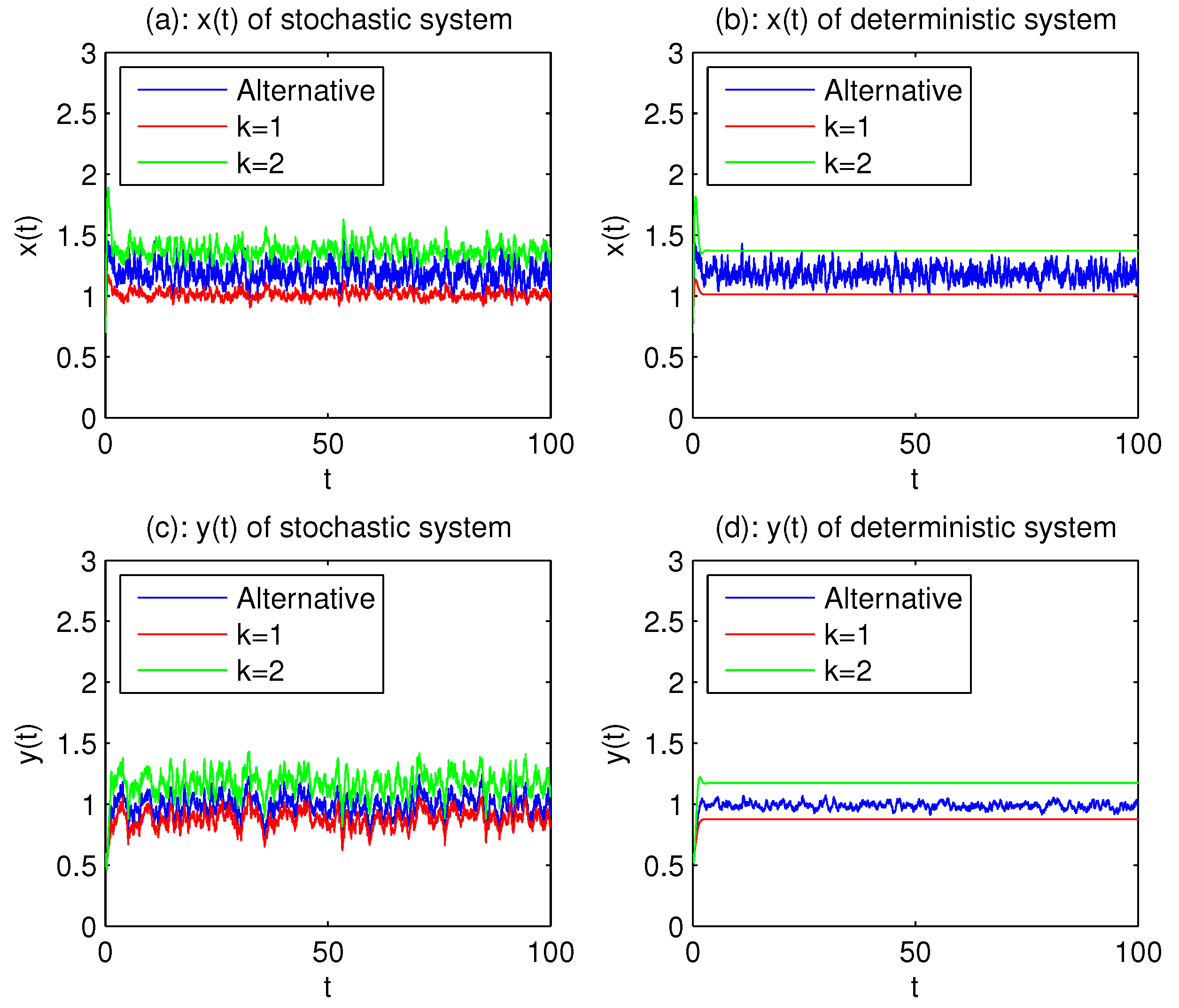
When we choose $({\sigma }_1\left(1\right),{\sigma }_1\left(2\right))=(0.07,0.08),({\sigma }_2\left(1\right),{\sigma }_2\left(2\right))=(0.09,0.06)$, this means that the two species are affected by smaller white noise. Since ${\sum }_{k=1}^2{\pi }_k[b_1\left(k\right)-\frac{{\sigma }_1^2\left(k\right)}{2}]\approx 7.58>0$ and $\overline{\kappa }=\frac{{\widehat{a}}_{21}}{{\check{a}}_{11}+\beta {\widehat{b}}_1}{\sum }_{k=1}^2{\pi }_k[{\widehat{b}}_1-\frac{{\sigma }_1^2\left(k\right)}{2}]-{\sum }_{k=1}^2{\pi }_k[b_2\left(k\right)+\frac{{\sigma }_2^2\left(k\right)}{2}]\approx 1.88>0$, from Theorem 2, SDE (3) has a unique stationary distribution, as shown Figure 1 and Figure 2.

Figure 1. The subgraphs (a,b) represent the sample phase portraits of the stochastic system (3) and the corresponding deterministic system, respectively. Three colors represent three states—$k=1,k=2$ and the alternative case—between them. The white noise intensities on $x\left(t\right)$ and $y\left(t\right)$ are relatively small. $({\sigma }_1\left(1\right),{\sigma }_1\left(2\right))=(0.07,0.08)$ and $({\sigma }_2\left(1\right),{\sigma }_2\left(2\right))=(0.09,0.06)$.

Figure 2. Representatively, the populations of $x\left(t\right)$ and $y\left(t\right)$ change over time in the states $k=1$, $k=2$ and the alternative case, respectively. The volatility of stochastic systems solutions is not great. $({\sigma }_1\left(1\right),{\sigma }_1\left(2\right))=(0.07,0.08)$ and $({\sigma }_2\left(1\right),{\sigma }_2\left(2\right))=(0.09,0.06)$.

The red, green, and blue colors represent the phase of x and y when they are in the states $k=1$, $k=2$ and switching back and forth from one state $k=1$ to another state $k=2$ according to the movement of $r\left(t\right)$, respectively. Figure 1 and Figure 2 show that the blue sandwiches between red and green are either deterministic or stochastic systems, which means that, when white noise is small, Markov switching helps to reduce the risk of species extinction. We can also see from Figure 1a that the three colored regions are all distributed in small areas, and in Figure 2a,c, the fluctuation of stochastic curves are gentle. From Figure 1 and Figure 2, one can clearly see the impact of small white noise and colored environment noise on populations.

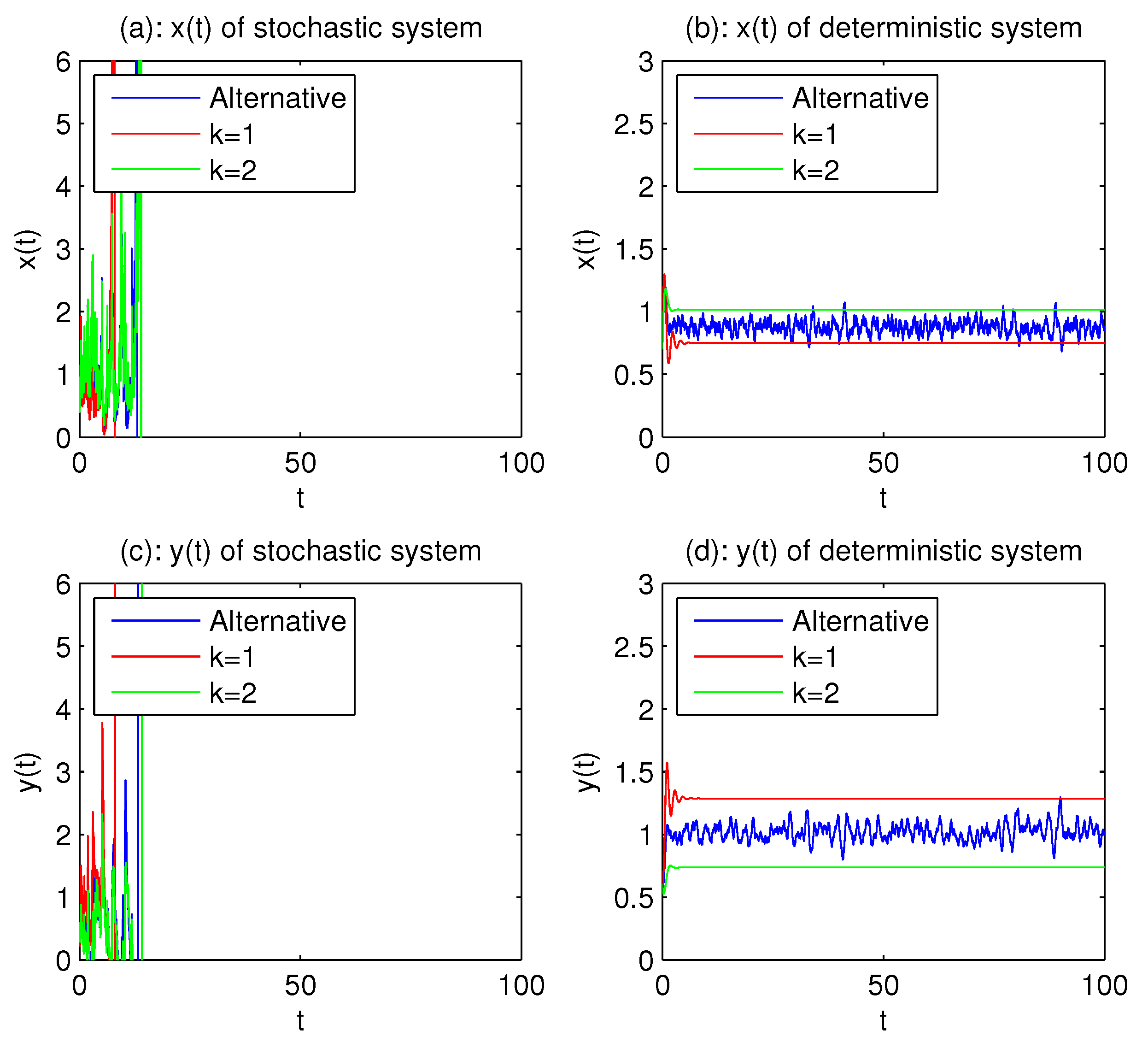
When we choose $({\sigma }_1\left(1\right),{\sigma }_1\left(2\right))=(1.7,1.9),({\sigma }_2\left(1\right),{\sigma }_2\left(2\right))=(1.5,1.7)$, then ${\sum }_{k=1}^2{\pi }_k[b_1\left(k\right)-\frac{{\sigma }_1^2\left(k\right)}{2}]\approx 6.7>0$ and $\overline{\kappa }\approx -0.09<0$; hence, assumption $\left(A\right)$ does not hold. Making use of Theorem 1 leads to the conclusion that both prey population x and predator population y go to extinction. Figure 3a and Figure 4a,c confirm this. Large white noise can lead to population extinction, even though the corresponding deterministic model is persistent (see Figure 3b and Figure 4b,d) and the existence of an ergodic.

Figure 3. The definitions of the subgraphs (a,b) are the same as in Figure 1. The big white noise intensity caused extinction of $x\left(t\right)$ and $y\left(t\right)$ as shown in (a). $({\sigma }_1\left(1\right),{\sigma }_1\left(2\right))=(1.7,1.9)$, $({\sigma }_2\left(1\right),{\sigma }_2\left(2\right))=(1.5,1.7)$.

Figure 4. The definitions of the subgraphs are the same as in Figure 2. $({\sigma }_1\left(1\right),{\sigma }_1\left(2\right))=(1.7,1.9)$, $({\sigma }_2\left(1\right),{\sigma }_2\left(2\right))=(1.5,1.7)$.

6. Conclusions and Future Directions

This paper discussed the properties of a stochastic predator–prey model with the Beddington–DeAngelis functional response. We investigated the strong persistence in the mean and the extinction of the SDE (3) with regime switching. The threshold between them was obtained. We also established the sufficient conditions for the existence of an ergodic stationary distribution of SDE (3) with regime switching. Our results suggest that the value of each coefficient and the intensity of white noise in $\kappa$ and $\overline{\kappa }$ determine the persistence and the extinction of a species, which is consistent with reality. The presence of the Markov chain in SDE (3) can contribute to the survival of the population, and reduce the risk of extinction when the white noise is not big.

At the theoretical level, the findings of this paper provide a theoretical basis for other biological predator–prey models with functional response, and competitive systems. The mathematical tools used in this paper may also be helpful for discussing 2-dimensional models of species interaction. At the biological application level, because the Beddington–DeAngelis functional response function has similar rate-dependent qualitative properties and there is no singularity in low population density regions, it can better describe predator–prey interactions, especially predator feeding. Environmental noise is ubiquitous in nature. Scholars usually use Brownian motion to explain the environmental white noise and Markov chain to represent the switching process. Their introduction can better describe the inevitable random interference of the population in nature. In other words, the model developed in this paper has universal and realistic significance. We envision that, in the future, with the establishment and improvement of relevant databases with which to record changes in species populations and environmental fluctuations, more data will be available for reference. The expression of the threshold value and the condition of the stationary distribution obtained in this paper can be used to monitor the quantitative change trend of species in nature reserves. When the monitored data exceeds the threshold, the protection mechanism can be enabled. The early warning can be lifted by controlling the intensity of white noise. Therefore, we hope that, in the future, under the right conditions, endangered species and biodiversity can be protected in this way.

References

- Perc, M.; Szolnoki, A.; Szab, G. Cyclical interactions with alliance-specific heterogeneous invasion rates. Phys. Rev. E 2007, 75, 052102. [Google Scholar] [CrossRef]
- Perc, M.; Szolnoki, A. Noise-guided evolution within cyclical interactions. New J. Phys. 2007, 9, 267. [Google Scholar] [CrossRef]
- Beddington, J.R. Mutual interference between parasites or predators and its effect on searching efficiency. J. Animal Ecol. 1975, 44, 331–341. [Google Scholar] [CrossRef]
- DeAngelis, D.L.; Goldsten, R.A.; Neill, R. A model for trophic interaction. Ecology 1975, 56, 881–892. [Google Scholar] [CrossRef]
- Skalski, G.T.; Gilliam, J.F. Functional responses with predator interference: Viable alternatives to the Holling type II model. Ecology 2001, 82, 3083–3092. [Google Scholar] [CrossRef]
- Cosner, C.; Deangelis, D.L.; Ault, J.S.; Olson, D.B. Effects of spatial grouping on the functional response of predators. Theor. Popul. Biol. 1999, 56, 65–75. [Google Scholar] [CrossRef]
- Wang, Y.; Lu, M.M.; Liu, J. Global stability of a delayed virus model with latent infection and Beddington–DeAngelis infection function. Appl. Math. Lett. 2020, 1007, 106463. [Google Scholar] [CrossRef]
- Ming, Q.; Yang, L.L. Steady state in a cross-diffusion predator–prey model with the Beddington–DeAngelis functional response. Nonlinear Anal. Real World Appl. 2019, 45, 401–413. [Google Scholar] [CrossRef]
- Fan, M.; Kuang, Y. Dynamics of a nonautonomous predator–prey system with the Beddington–DeAngelis functional response. J. Math. Anal. Appl. 2004, 295, 15–39. [Google Scholar] [CrossRef]
- Lin, X.; Chen, F. Almost periodic solution for a Volterra model with mutual interference and Beddington–DeAngelis functional response. Appl. Math. Comput. 2009, 214, 548–556. [Google Scholar] [CrossRef]
- Guo, H.J.; Chen, X.X. Existence and global attractivity of positive periodic solution for a Volterra model with mutual interference and Beddington–DeAngelis functional response. Appl. Math. Comput. 2011, 217, 5830–5837. [Google Scholar] [CrossRef]
- Wang, X.T.; Zhao, M. Chaos in a Hybrid Three-Species Food Chain with Beddington–DeAngelis Functional Response. Procedia Environ. Sci. 2011, 10, 128–134. [Google Scholar] [CrossRef]
- Wang, Z.; Wang, Y. Bifurcations in diffusive predator–prey systems with Beddington–DeAngelis functional response. Nonlinear Dyn. 2021, 105, 1045–1061. [Google Scholar] [CrossRef]
- Hwang, T.W. Uniqueness of limit cycles of the predator–prey system with Beddington–DeAngelis functional response. J. Math. Anal. Appl. 2004, 290, 113–122. [Google Scholar] [CrossRef]
- Baek, H. Qualitative analysis of Beddington–DeAngelis type impulsive predator–prey models. Nonlinear Anal. Real World Appl. 2010, 11, 1312–1322. [Google Scholar] [CrossRef]
- Li, H.; Cheng, X. Dynamics of Stage-Structured Predator–Prey Model with Beddington–DeAngelis Functional Response and Harvesting. Mathematics 2021, 9, 2169. [Google Scholar] [CrossRef]
- Dimitrov, D.; Kojouharov, H. Complete mathematical analysis of predator–prey models with linear prey growth and Beddington–DeAngelis functional response. Appl. Math. Comput. 2005, 162, 523–538. [Google Scholar] [CrossRef]
- Xu, C.; Wang, M. Permanence for a delayed discrete three-level food-chain model with Beddington–DeAngelis functional response. Appl. Math. Comput. 2007, 187, 1109–1119. [Google Scholar] [CrossRef]
- Ko, W.; Ryu, K. Analysis of diffusive two-competing-prey and one-predator systems with Beddington–DeAngelis functional response. Nonlinear Anal. 2009, 71, 4185–4202. [Google Scholar] [CrossRef]
- Li, H.; Takeuchi, Y. Dynamics of the density dependent predator–prey system with Beddington–DeAngelis functional response. J. Math. Anal. Appl. 2011, 374, 644–654. [Google Scholar] [CrossRef]
- Ji, C.Y.; Jiang, D.Q. Dynamics of a stochastic density dependent predator–prey system with Beddington–DeAngelis functional response. J. Math. Anal. Appl. 2011, 381, 441–453. [Google Scholar] [CrossRef]
- Qiu, H.; Liu, M.; Wang, K.; Wang, Y. Dynamics of a stochastic predator–prey system with Beddington–DeAngelis functional response. Appl. Math. Comput. 2012, 219, 2303–2312. [Google Scholar] [CrossRef]
- Yagi, A.; Viet, T.T. Dynamic of a stochastic predator–prey population. Appl. Math. Comput. 2011, 218, 3100–3109. [Google Scholar] [CrossRef]
- Ji, C.Y.; Jiang, D.Q.; Shi, N.Z. A note on a predator–prey model with modified Leslie-Gower and Holling-type II schemes with stochastic perturbation. J. Math. Anal. Appl. 2011, 377, 435–440. [Google Scholar] [CrossRef]
- Liu, M.; Wang, K. Global stability of a nonlinear stochastic predator–prey system with Beddington–DeAngelis functional response. Commun. Nonlinear Sci. Numer. Simulat. 2011, 16, 1114–1121. [Google Scholar] [CrossRef]
- Li, X.Y.; Gray, A.; Jiang, D.Q.; Mao, X.R. Sufficient and necessary conditions of stochastic permanence and extinction for stochastic logistic populations under regime switching. J. Math. Anal. Appl. 2011, 376, 11–28. [Google Scholar] [CrossRef]
- Li, X.Y.; Jiang, D.Q.; Mao, X.R. Population dynamical behavior of Lotka-Volterra system under regime switching. J. Comput. Appl. Math. 2009, 232, 427–448. [Google Scholar] [CrossRef]
- Liu, M.; Wang, K. Dynamics of a Leslie-Gower Holling-type II predator–prey system with Le´vy jumps. Nonlinear Anal. 2013, 85, 204–213. [Google Scholar] [CrossRef]
- Mao, X.R.; Yuan, C.G. Stochastic Differential Equations with Markovian Switching; Imperial College Press: London, UK, 2006. [Google Scholar]
- Mao, X.; Marion, G.; Renshaw, E. Environmental noise suppresses explosion in population dynamics. Stoch. Process. Appl. 2002, 97, 95–110. [Google Scholar] [CrossRef]
- Mao, X. Stationary distribution of stochastic population systems. Syst. Control. Lett. 2011, 60, 398–405. [Google Scholar] [CrossRef]
- Zu, L.; Jiang, D.Q.; O’Regan, D.; Hayat, T.; Ahmad, B. Ergodic property of a Lotka–Volterra predator–prey model with white noise higher order perturbation under regime switching. Appl. Math. Comput. 2018, 330, 93–102. [Google Scholar] [CrossRef]
- Jiang, X.B.; Zu, L.; Jiang, D.Q.; O’Regan, D. Analysis of a Stochastic Holling Type II Predator–Prey Model Under Regime Switching. Bull. Malays. Math. Sci. Soc. 2020, 43, 2171–2197. [Google Scholar] [CrossRef]
- Zu, L.; Jiang, D.Q.; O’Regan, D.; Hayat, T. Dynamic analysis of a stochastic toxin-mediated predator-prey model in aquatic environments. J. Math. Anal. Appl. 2021, 504, 125424. [Google Scholar] [CrossRef]
- Liu, H.; Li, X.X.; Yang, Q.S. The ergodic property and positive recurrence of a multi-group Lotka-Volterra mutualistic system with regime switching. Syst. Control Lett. 2013, 62, 805–810. [Google Scholar] [CrossRef]
- Settati, A.; Lahrouz, A. Stationary distribution of stochastic population systems under regime switching. Appl. Math. Comput. 2014, 244, 235–243. [Google Scholar] [CrossRef]
- Zhu, C.; Yin, G. Asymptotic properties of hybrid diffusion systems. SIAM J. Control Optim. 2007, 46, 1155–1179. [Google Scholar] [CrossRef]
- Zhu, C.; Yin, G. On competitive Lotka-Volterra model in random environments. J. Math. Anal. Appl. 2009, 357, 154–170. [Google Scholar] [CrossRef]
- Zu, L.; Jiang, D.Q.; O’Regan, D. Conditions for persistence and ergodicity of a stochastic Lotka-Volterra predator–prey model with regime switching. Commun. Nonlinear Sci. Numer. Simulat. 2015, 29, 1–11. [Google Scholar] [CrossRef]
- Liu, M.; Wang, K.; Wu, Q. Survival analysis of stochastic competitive models in a polluted environment and stochastic competitive exclusion principle. Bull. Math. Biol. 2011, 73, 1969–2012. [Google Scholar] [CrossRef]
- Bibi Ruhomally, Y.; Zaid Dauhoo, M.; Dumas, L. Stochastic modelling of marijuana use in Washington: Pre-and post-Initiative-502 (I-502). IMA J. Appl. Math. 2022, 87, 1121–1150. [Google Scholar] [CrossRef]
- Lahrouz, A.; Omari, L. Extinction and stationary distribution of a stochastic SIRS epidemic model with non-linear incidence. Stat. Probab. Lett. 2013, 83, 960–968. [Google Scholar] [CrossRef]
- Ruan, S.; Xiao, D. Global analysis in a predator–prey system with nonmonotonic functional response. SIAM J. Appl. Math. 2001, 61, 1445–1472. [Google Scholar]
- Khasminskii, R.Z.; Zhu, C.; Yin, G. Stability of regime-switching diffusions. Stoch. Process. Appl. 2007, 117, 1037–1051. [Google Scholar] [CrossRef]
- Higham, D.J. An algorithmic introduction to numerical simulation of stochastic differential equations. SIAM Rev. 2001, 43, 525–546. [Google Scholar] [CrossRef]
Disclaimer/Publisher’s Note: The statements, opinions and data contained in all publications are solely those of the individual author(s) and contributor(s) and not of MDPI and/or the editor(s). MDPI and/or the editor(s) disclaim responsibility for any injury to people or property resulting from any ideas, methods, instructions or products referred to in the content. |
© 2023 by the authors. Licensee MDPI, Basel, Switzerland. This article is an open access article distributed under the terms and conditions of the Creative Commons Attribution (CC BY) license (https://creativecommons.org/licenses/by/4.0/).