A Multi-Agent Adaptive Co-Evolution Method in Dynamic Environments

Abstract

It is challenging to ensure satisfying co-evolution efficiency for the multi-agents in dynamic environments since during Actor-Critic training there is a high probability of falling into local optimality, failing to adapt to the suddenly changed environment quickly. To solve this problem, this paper proposes a multi-agent adaptive co-evolution method in dynamic environments (ACE-D) based on the classical multi-agent reinforcement learning method MADDPG, which effectively realizes self-adaptive new environments and co-evolution in dynamic environments. First, an experience screening policy is introduced based on the MADDPG method to reduce the negative influence of original environment experience on exploring new environments. Then, an adaptive weighting policy is applied to the policy network, which accordingly generates benchmarks for varying environments and assigns higher weights to those policies that are more beneficial for new environments exploration, so that to save time while promoting adaptability of the agents. Finally, different types of dynamic environments with complexity at different levels are built to verify the co-evolutionary effects of the two policies separately and the ACE-D method comprehensively. The experimental results demonstrate that, compared with a range of other methods, the ACE-D method has obvious advantages helping multi-agent adapt to dynamic environments and preventing them from falling into local optima, with more than 25% improvement in stable reward and more than 23% improvement in training efficiency. The ACE-D method is valuable and commendable to promote the co-evolutionary effect of multi-agent in dynamic environments.

1. Introduction

Co-evolution is used to realize collaboration between multi-agent [1] dealing with complex task environments. At present, most of the multi-agent co-evolution methods are based on stable and static environments with which the agents therein interact so that to generate experiences and learn to adapt to the environment gradually, such as the ISGE-NCE method and MPT-NCE method based on non-cooperative equilibrium [2,3]. However, in a dynamic environment where the task conditions are constantly changing, the best policy made by the agents based on the current information would no longer be the ‘best’ as the environment changes [4]. Take the scene of chasing for instance; the number and position of the agents, obstacles and targets, the obstacle motion mode, and any change of these factors lead to a dynamic environment. With this understanding, the optimal parameters learned for the agents based on the original experience obtained from previous environment may become over-fitting as a set of local optimal solutions [5]. In this case, to restart the training is a straight way to avoid the local optimum but is time-consuming. To realize quick adaptive co-evolution of a multi-agent within dynamic environments, it is of great significance to solve the problem of a possible local optimum in the process of learning and evolution of the multi-agent.

In recent years, the exploration of a dynamic environment has been carried out in many applications, such as robot navigation in a dynamic environment [6] and a patrol task in a dynamic environment [7]. Transfer learning is a common method for solutions in those works, owning the advantage of timesaving for multi-agent learning to adapt to environmental changes [8], by using negotiation and knowledge transfer methods to cope with environment changes [9,10], by combining the concept of incremental learning with the dynamic environment in the evolutionary strategies [11], by adopting a scalable transfer learning framework to solve dynamic environments [12], by using neural networks to transmit information on changes in the environment [13], and by using the deep convolutional transfer learning model (DCTL) to cope with changing tasks [14]. In addition to transfer learning, Q learning [15,16] has also been used to solve random dynamic environments successfully. The combination of table Q learning and transfer learning [17] also presented excellent performance in highly dynamic emergencies. The above methods show their capacity to cope with a dynamic environment in a low-dimensional continuous action space to some extent; however, it is still challenging to transfer knowledge between different environments [18]. In the actual environment, the action space is often high-dimensional, and the reinforcement learning (RL) in the high-dimensional space is often plagued by the curse of dimensionality. The number of parameters to be learned increase exponentially with the increase of environmental complexity [19]. In the high-dimensional action space, frequent sampling and integration are very computationally intensive, especially in the multi-agent field. The increase in the number of agents will significantly affect the robustness of the environment exploration.

Many methods for solving high-dimensional action space have been proposed in recent decades. For example, the Deterministic Policy Gradient (DPG) [20], whose policies are deterministic, requiring no sampling integration in the action space, greatly cutting the required sample data, thus improving the computational efficiency. The Deep Deterministic Policy Gradient (DDPG) algorithm combines the advantages of DPG and Deep Q Network (DQN), for which as a basis, the ‘Actor-Critic’ framework is introduced additionally to realize real-time tracking [21,22] and dynamic programming of autonomous driving [23,24,25], as well as some other dynamic problems. The traditional RL method is difficult to be used for multi-agent, because the policy of each agent is constantly changing during the training process, which would cause the environment to be unstable; apparently the policy learned in an unstable environment is meaningless. For multi-agent systems, a consensus for a generic linear multi-agent system with heterogeneous inputs and communication delays is proposed [26]. Knowledge reuse for multi-agent systems is studied [27]. MADDPG is a classical algorithm in the field of multi-agent, and by extending DDPG to the field of multi-agent, MADDPG realizes the co-evolution of multi-agent and solves the problem of flocking control in dynamic obstacle environment [28]. On this basis, the MiniMax Multi-agent Deep Deterministic Policy Gradient (M3DDPG) [29], which can achieve generalization when the opponent’s policy changes, and the ATT-MADDPG algorithm [30], which adaptively models the dynamic joint policy of teammates, are also proposed. The multi-agent time delay deep deterministic policy gradient (TD3) reduces the overestimation error of neural network approximation and the variance of estimation results by means of policy updating delay, so that it improves the ability of agents to adapt to complex tasks [31]. The MADDPG algorithm is applied to the control of unsignalized traffic intersections, in which a partial static environment is constructed by selecting reference vehicles to solve the problem of dynamic vehicles in the real environment [32]. A temporal convolutional network (TCN) model for modeling and predicting adversary behavior, the OM-TCN, is proposed to cope with the environmental non-stationarity caused by adversary policy changes [33]. The ESB-MADDPG method for swarm robots can improve the decision-making ability of the multi-agent [34]. Compared with MADDPG, the above methods pay more attention to improving the ability of multi-agent to adapt to complex tasks or enhancing robustness and have good performance in static environment testing. However, the existing research rarely involves the co-evolution of a multi-agent in a dynamic environment and has not been tested thoroughly in dynamic environments.

This paper proposes a multi-agent adaptive co-evolution method in a dynamic environment, which aims to improve the ability of multi-agent to adapt to a dynamic environment, enhance the capacity of a multi-agent to get rid of local optimum, improve the speed of the multi-agent to adapt to a new environment, and finally realize the adaptive co-evolution of the multi-agent in different dynamic environments. On the premise that the experience has been learned from the original environment, the policies experience screening (ES) and adaptive weighting (AW) are proposed. First of all, some experiences obtained from original environments would affect the adaptation of multi-agent to the new environment, and the agents need to eliminate such interference as much as possible. The experience screening policy separates the experience into that of the old and new environments and then screens the experience of the new environment to guide the agents correctly explore and quickly adapt to the new environment. Secondly, prioritizing the action learning of which that performs better is conducive to adapting to the new environment, but different dynamic environments have different benchmarks for judging the advantages and disadvantages of actions. The adaptive weighting policy selects actions that are more worthy of priority learning and to higher weights according to the adaptive generation benchmarks of the environment, encouraging the replacement of the originally optimal actions with new actions that are more adapted to the new environment as soon as possible. Experience screening and adaptive weighting work together to realize the adaptive co-evolution function of a multi-agent in a dynamic environment. Finally, experiments are designed and carried out with different dynamic environments for methods evaluation, and the adaptability of the proposed method in different types of dynamic environments is verified.

2. Related Work

2.1. Dynamic Environment

A dynamic environment means that in the process of training, the environment is not static, but changes at a certain moment. Therefore, the dynamic environment is regarded as a series of continuous fixed tasks along the time scale, and each task has corresponding environmental characteristics at certain time period. Assume that the dynamic environment $S$ includes different tasks $M_t$ in different time periods, that is, $S=\{M_1,M_2,\dots ,M_t,M_{t+1},\dots \}$, where $M_t\in M$ represents the task in the $t$ time period [4].

The initial training parameter is assumed to be ${\theta }_0$. The task in the t time period is $M_t$, and the optimal parameter learned by the agent is ${\theta }_t$; when the task is changed to $M_{t+1}$ in the $t+1$ time period, the optimal parameter will be changed to ${\theta }_{t+1}$. The new environment is not completely different from the initial environment, and there is a certain connection between them. The optimal parameters $\left({\theta }_t,{\theta }_{t+1},{\theta }_{t+2},\cdots \right)$ are gradually changed with the dynamic changes of the environment, so there is also a connection between the optimal parameters. Using this connection, it is more advantageous to adapt to the new environment on the basis of the original environment (${\theta }_{t+1}\leftarrow {\theta }_t$, ${\theta }_{t+2}\leftarrow {\theta }_{t+1}$) than to retrain (${\theta }_{t+1}\leftarrow {\theta }_0$, ${\theta }_{t+2}\leftarrow {\theta }_0$).

2.2. MADDPG Algorithm

The MADDPG algorithm is a deep learning model with the AC architecture and is an extension of DDPG in multi-agent tasks. Its core idea is to centralize training and decentralize execution. Each agent has its corresponding policy network and critic network. The input of the policy network is the current state $S_t$; the output is the determined policy $A_t$ and interacts with the environment to generate the next moment state $S_{t+1}$. The critic network judges the value of the policy and outputs the evaluation $Q$. The learning purpose of the policy network is to obtain a larger $Q$ value, and the learning purpose of the critic network is to reduce the error between the actual $Q$ value and the approximate evaluation $y_t$.

The “centralized training, decentralized execution” of MADDPG is to use the experience of all agents during training, and each agent uses its own observations to obtain policies separately during execution. The critic network contains observations and actions of all agents. The loss function of the critic network is evaluated as Equation (1):

$$L=\frac{1}{K}{\sum }_{t=1}^K{(y_t-Q(S_t,A_t,{\theta }^Q\left)\right)}^2,$$

(1)

where ${\theta }^Q$ is the critic network parameter, and $Q(S_t,A_t,{\theta }^Q)$ is the actual $Q$ value of the critic network output. The approximate evaluation $y_t$ at the next moment is obtained by Equation (2).

$$y_t=R_t+\gamma Q^{\prime }\left(S_{t+1},A_{t+1},{\theta }^{Q^{\prime }}\right),$$

(2)

where $\gamma$ is the discount factor and $Q^{\prime }$ is the predicted $Q$ value of the target critic network output.

The gradient calculation formula of the policy network is as Equation (3)

$${\nabla }_{{\theta }^u}J=\frac{1}{K}{\sum }_{t=1}^K{\nabla }_{{\theta }^u}\pi (S_t,{\theta }^u)\nabla Q(S_t,A_t,{\theta }^Q),$$

(3)

where ${\theta }^u$ is the policy network parameter. MADDPG uses delayed updates, so the data in the above equations are randomly sampled from the experience replay buffer.

2.3. Prioritized Experience Replay

The update of the critic network is achieved by calculating the gap between the actual $Q$ value and the approximate evaluation $y_t$. Therefore, the larger the difference $\delta =y_t-Q$, the higher the value. Therefore, the priority experience replay method is adopted to update the array with a larger $\delta$ value [35]. The probability of each array being extracted is set according to the size of $\delta$. The probability is shown in Equation (4):

$$p_j=\left|\delta \right|+ϵ,$$

(4)

where $ϵ$ is a small number; the probability of preventing data from being extracted is 0. Normalization is shown in Equation (5):

$$P_j=\frac{{p_j}^{\alpha }}{{\sum }_k{p}_k^a}.$$

(5)

The weight of each experience is calculated by Equation (6):

$${\omega }_k=\frac{1}{{\left(X·P_j\right)}^{\mu }},$$

(6)

where $X$ is the capacity of the replay buffer. The loss function of the critic network becomes Equation (7):

$$L=\frac{1}{K}{\sum }_{k=1}^K{{\omega }_k(y_t-Q(s_t,a_1,a_2,\dots ,a_N,{\theta }^Q\left)\right)}^2.$$

(7)

The principle of Prioritized Experience Replay is to find out the data with a larger gap between the predicted value and the actual value through the time difference (TD) method. Such data indicate inaccurate predictions and have a higher learning value and need to be prioritized, therefore giving these data a higher probability of being selected.

3. Methodology of This Article

This section first introduces the classification of dynamic environments, then describes in detail the experience screening and adaptive weighting policies proposed in this paper, and finally gives a multi-agent adaptive co-evolution method in dynamic environments based on the above policies. Among them, Section 3.1 is about the experience screening; Section 3.2 is about the adaptive weighting, and Section 3.3 is about the proposed multi-agent adaptive co-evolution method ACE-D in dynamic environments.

The dynamic environment is the environmental state in different time periods, and the dynamic changes of its self-environment and the external environment cause the diversity of the dynamic environment. The self-environment studied in this paper mainly refers to the dynamic changes of the initial position, number, and motion mode of the agent. The external environment mainly refers to the dynamic changes of the initial position, number, and motion mode of the obstacle. In addition, the dynamic environment in this paper maintains the same state space and action space; only the agent and the obstacle change dynamically.

Once the environment changes, it is undoubtedly more beneficial to continue learning on the basis of the optimal parameters inherited from the original environment, while aiming to adapt to the new environment. However, at this time, the experiences of both original environment and new environment are mixed in the experience replay buffer. Since the agents have been trained in the original environment, its own critic criterion would be formed more biased towards the policy that suits the original environment. Especially in the process of interactive learning with the new environment, the data extracted from the replay buffer contain the original environment information, which further affects the agent’s discrimination of better policies for the new environment. In addition, the agent’s policy is the only deterministic policy generated by the policy network. The agent is likely to fail in finding a better alternative policy in the new environment but fall into a state of overfitting; that is, it is easier to be locally optimal.

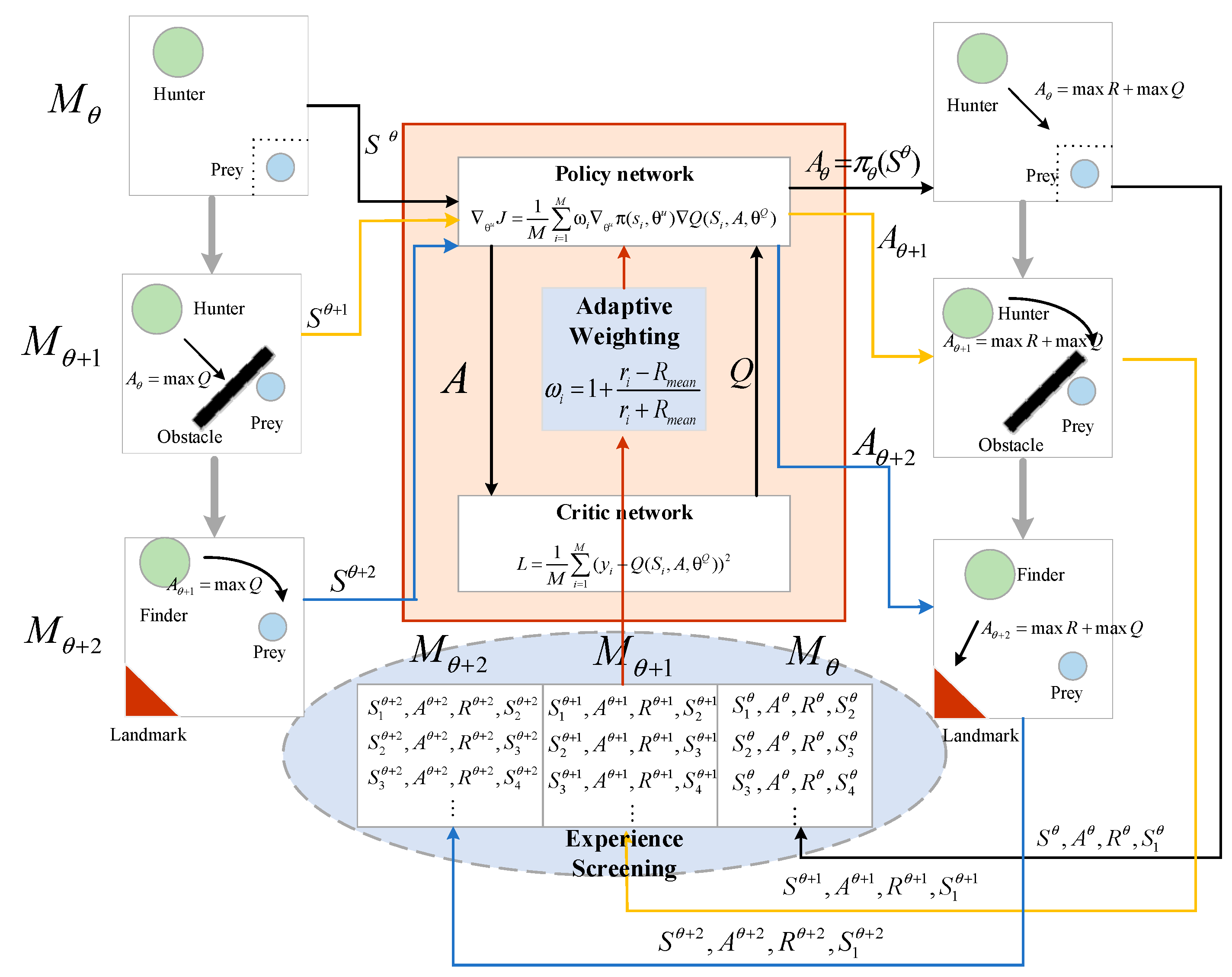
Based on this, this paper proposes a multi-agent adaptive co-evolution method in a dynamic environment. As shown in Figure 1, the multi-agent learns the optimal action $A_{\theta }$ in the original environment $M_{\theta }$ through the policy network and the critic network. Since then, the environment has changed dynamically to $M_{\theta +1}$, and the action $A_{\theta }$ can still obtain a high $Q$ value from the critic network, but it is not the optimal action in $M_{\theta +1}$. At this time, the experience screening and adaptive weighting policies are enabled to help the multi-agent adjust $A_{\theta }$ to the optimal action $A_{\theta +1}$ in $M_{\theta +1}$. The experience screening policy distinguishes the experience of the original environment and furtherly eliminates the interference of them, then keeping only the experience of the new environment, so as to reduce the time spent on adapting to the new environment and avoid falling into the local optimum. The adaptive weighting policy adaptively allocates weights according to the rewards of actions in the new environment, avoiding the critic network continuously giving $A_{\theta }$ a high $Q$ value but ignoring other better actions in the new environment. By giving high weights to these preferred actions, the agents can quickly adapt to the new environment and prevent falling into local optimum. When the environment continues to change to $M_{\theta +2}$, the above process is repeated to quickly adapt to the new environment and learn the optimal action $A_{\theta +2}$.

3.1. Experience Screening (ES)

The replay buffer D of MADDPG is

$$S_t,a_1^t,a_2^t,\dots ,a_N^t,r_1^t,r_2^t,\dots ,r_N^t,S_{t+1}.$$

The experience replay buffer continuously stores experience and deletes the very previous experience when the buffer reaches its storage upper limit. As the environment changes, the experience of the old and new environments would coexist in the experience replay buffer.

Therefore, after the environment changes, it is assumed that totally $K$ sets of experience are extracted from the replay buffer $D$, where $N$ sets are the experience of the original environment and $M$ sets are of the new environment. Since experience is randomly extracted from the experience replay buffer, the order of experience in the original environment and the new environment is random; thus, $N$ and $M$ only represent the amount but not the order of experience. The policy network is updated as Equation (8):

$$\begin{gathered} {\nabla }_{{\theta }^u}J=\frac{1}{K}\left({\sum }_{t=1}^N{\nabla }_{{\theta }^u}\pi \left(s_t,{\theta }^u\right)\nabla Q\left(s_t,a_1,a_2,\dots ,a_N,{\theta }^Q\right)\right.+ \\ {\sum }_{i=N+1}^{M+N}{\nabla }_{{\theta }^u}\pi (s_i,{\theta }^u)\nabla Q(s_i,a_1,a_2,\dots ,a_N,{\theta }^Q)). \end{gathered}$$

(8)

Critic network updates as Equation (9):

$$L=\frac{1}{K}\left({\sum }_{t=1}^N{(y_t-Q(s_t,a_1,a_2,\dots ,a_N,{\theta }^Q\left)\right)}^2+{\sum }_{i=N+1}^{M+N}{(y_i-Q(s_i,a_1,a_2,\dots ,a_N,{\theta }^Q\left)\right)}^2\right).$$

(9)

It can be seen from Equations (8) and (9) that after the environment changes, the experience of the original environment would keep affecting the multi-agent, which is not applicable for agents learning to adapt to new environment. These experiences will inevitably adversely affect the learning process of the multi-agent, reduce the efficiency of the multi-agent to adapt to the new environment, and even lead to a local optimum. How to avoid an unfavorable old experience has become a problem waiting to be solved. The essence of prioritized experience replay is to select more valuable experience that contains more information. In a dynamic environment, the learnability of the new environment is much higher than that of the original environment. It is more conducive to quickly adapt to the new environment by abandoning the old experience and directly learning the experience of the new environment based on the original model. Prioritized experience replay assigns weights to experiences through TD method. Low weight goes to old experience offering low learning value, so to reduce the effect of these experiences to a certain extent. However, the prioritized experience replay method needs to traverse the replay buffer when fixing the weights, which takes a lot of time and greatly increases the training time.

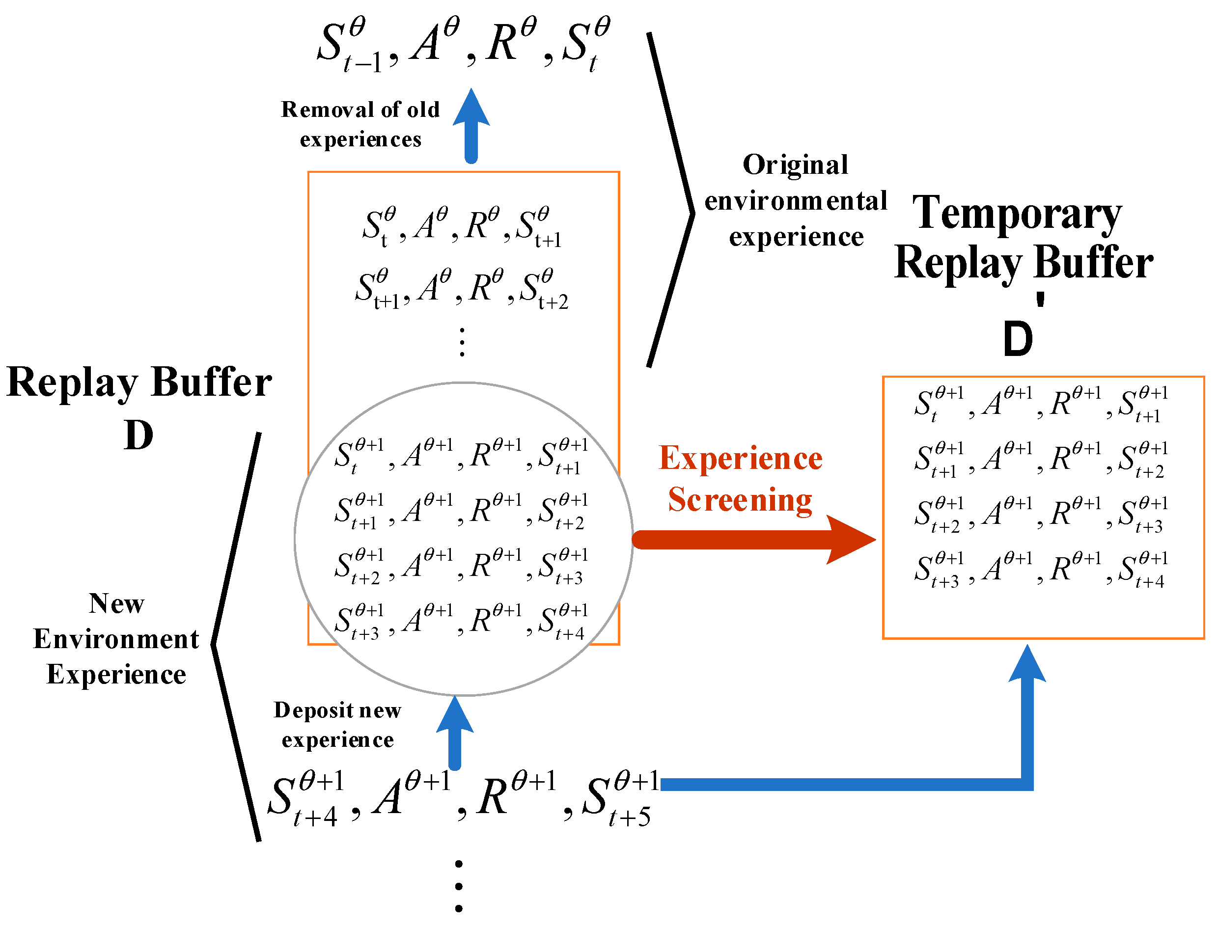
As shown in Figure 2, the experience screening policy establishes a temporary replay buffer $D^{\prime }$. As the environment changes dynamically, the experience in the new environment is stored in the temporary replay buffer $D^{\prime }$ and is extracted from $D^{\prime }$ to participate in the update of the critic network. The updating of the policy network is carried out in accordance with Equation (10), and the updating of the critic network is executed as Equation (11). At this time, $K=M$:

$${\nabla }_{{\theta }^u}J=\frac{1}{M}{\sum }_{i=1}^M{\nabla }_{{\theta }^u}\pi \left(s_i,{\theta }^u\right)\nabla Q\left(s_i,a_1,a_2,\dots ,a_N,{\theta }^Q\right),$$

(10)

$$L=\frac{1}{M}{\sum }_{i=1}^M{(y_i-Q(s_i,a_1,a_2,\dots ,a_N,{\theta }^Q\left)\right)}^2.$$

(11)

The temporary replay buffer $D^{\prime }$ will not be disturbed by the information of the original environment, and the data in the experience replay buffer $D$ will gradually be replaced by the experience of the new environment. After the experience replay buffer $D$ is full of new environmental experience, it begins to extract data from $D$, and the temporary replay buffer $D^{\prime }$ is emptied, waiting for the next environmental change. The experience screening policy separates the old and new experiences and prioritizes learning the experience of the new environment, which eliminates the interference of unfavorable old experience and increases the efficiency of multi-agent adaptation to the new environment.

3.2. Adaptive Weighting (AW)

MADDPG adopts the deterministic policy, that is, $A_t={\pi }_{\theta }(S_t,{\theta }^u)$. Action $A_t$ is the only deterministic optimal policy under the environment $S_t$, and ${\theta }^u$ is the optimal parameter to adapt to the environment $S_t$. When the environment $S_t$ changes to the new environment $S_m$, the optimal parameter for the new environment would not keep being ${\theta }^u$; therefore, the policy generated by ${\theta }^u$ might not be the optimal policy facing the new environment. In this case, the unique certainty of the deterministic policy actually would hinder the agent learning and exploring the new environment effectively.

It can be seen from Equation (3) that the update of the policy network is related to the $Q$ value of the critic network, and the policy updates willing to obtain a higher $Q$ value from the critic network; consequently, the action recommended by the policy network would be inclined to increase the $Q$ value of the critic network rather than to increase the reward. When the environment changes, the parameters of the critic network are still the optimal parameters for the original environment, so it is still biased towards the optimal action for the original environment, with high likelihood to ignore the new action that offers higher rewards in the new environment. That is easy to result in the inaccuracy of the $Q$ value derived by the critic network in the new environment; in other words, it is not appropriate to evaluate the action only by $Q$ value. Therefore, an adaptive weighting policy is proposed, which introduces both the reward and $Q$ value as a new form of critic criterion to guide multi-agent learning of the actions to perform better in the new environment, helping the multi-agent adapt to the new environment and prevent falling into local optimum.

In the adaptive weighting policy, once the environment changes, the value of the action is judged according to the policy randomly selected in the replay buffer together with the corresponding reward, and the weight $\omega$ is calculated simultaneously. The optimal policy for the same environment differs at different stages, as does the optimal policy for different environments at the same stage and their corresponding rewards. Therefore, it is necessary to adjust the value of the policy according to the situation of the environment. Notice that it is not realistic to set a fixed benchmark artificially. Therefore, this paper proposes to adaptively generate and automatically adjust the decision benchmark according to the environmental parameters. That is to select the average reward $mean$ of the previous training, saying the $k_n~k_{n+m}$ sets training of the current environment, as the benchmark, and to adjust the benchmark automatically with the period of $m$ sets. The policy network update is shown as Equation (12):

$${\nabla }_{{\theta }^u}J=\frac{1}{M}{\sum }_{i=1}^M{\omega }_i{\nabla }_{{\theta }^u}\pi \left(s_i,{\theta }^u\right)\nabla Q(s_i,a_1,a_2,\dots ,a_N,{\theta }^Q),$$

(12)

where ${\omega }_i$ is the weight calculated adaptively according to the current reward of the action ${rew}_i$, as shown in Equation (13):

$${\omega }_i=1+\frac{{rew}_i-mean}{{rew}_i+mean}.$$

(13)

When ${rew}_i>mean$, the weight ${\omega }_i$ is positive and becomes concerned in learning. When ${rew}_i<mean$, the weight ${\omega }_i$ is negative, and the reward of the policy is already lower than the average reward at this time and therefore does not need to be focused in learning. When the interactive environment converges, the reward has also reached stability, at which time ${\omega }_i\approx 0$. In addition, this paper specifies the boundary of ${\omega }_i$ to prevent the cases when special sets of $rew$ and $mean$ drive the ${\omega }_i$ beyond the range of (−1, 1), when ${\omega }_i>1$, ${\omega }_i$ is randomly taken from (0, 1), and when ${\omega }_i<-1$, ${\omega }_i$ is randomly taken from (−1, 0).

3.3. Multi-Agent Adaptive Co-Evolution Method in Dynamic Environments (ACE-D)

The multi-agent adaptive co-evolutionary method in dynamic environments, the proposed ACE-D, distinguishes the experiences of the old and new environments through experience screening policy and selects those more valuable experiences for learning through adaptive weighting policy to help the multi-agent quickly adapt to the new environment and achieve co-evolution. The dynamic environment $S=\{M_1,M_2,\dots M_T\}$ is defined, and the time period that the task $M_T$ occupied is $T$ ($T\ge 1$). It is assumed that the original policy network parameter is ${\theta }^u$, the critic network parameter is ${\theta }^Q$, the network parameters in the training process are ${\theta }_t^u$ and ${\theta }_t^Q$, and the optimal parameters learned by the agents in $M_T$ are ${\theta }_T^u$ and ${\theta }_T^Q$. The ACE-D method is presented by Equations (14) and (15):

Policy network updates:

$${\nabla }_{{\theta }^u}J=\left\{\begin{array}{c}\\ \frac{1}{M}{\displaystyle \sum _{i=1}^M}{\omega }_i{\nabla }_{{\theta }^u}\pi \left(s_i,{\theta }^u\right)\nabla Q\left(s_i,a_1,a_2,\dots ,a_N,{\theta }^Q\right)\left(\mathrm{T}\ne 1 \mathrm{a}\mathrm{n}\mathrm{d} {\theta }_t^u\ne {\theta }_T^u,{\theta }_t^Q\ne {\theta }_T^Q\right)\\ \frac{1}{K}{\displaystyle \sum _{t=1}^K}{\nabla }_{{\theta }^u}\pi (s_t,{\theta }^u)\nabla Q(s_t,a_1,a_2,\dots ,a_N,{\theta }^Q)\left(\mathrm{else}\right)\end{array},\right.$$

(14)

critic network updates:

$$L=\left\{\begin{array}{c}\frac{1}{M}{\sum }_{i=1}^M{\left(y_i-Q\left(s_i,a_1,a_2,\dots ,a_N,{\theta }^Q\right)\right)}^2\left(\mathrm{T}\ne 1\mathrm{a}\mathrm{n}\mathrm{d}{\theta }_t^u\ne {\theta }_T^u,{\theta }_t^Q\ne {\theta }_T^Q\right)\\ \frac{1}{K}{\sum }_{t=1}^K{(y_t-Q(s_t,a_1,a_2,\dots ,a_N,{\theta }^Q\left)\right)}^2\left(\mathrm{else}\right)\end{array}\right.,$$

(15)

where $K$ is the number of experience sets extracted from the replay buffer $D$ during network update, $M$ is the number of experience sets extracted from the temporary replay buffer $D^{\prime }$, and ${\omega }_i$ is the weight calculated by Equation (13). The pseudo-code of ACE-D is shown in

Table 1. The pseudo-code of the ACE-D method.

pseudo-code

Initialize the dynamic environment $S=\left\{M_1,M_2,\dots M_T\right\}$$\mathrm{and} \mathrm{task} M_T$ occupies the time period of $T(T\ge 1)$. Setting the environmental change at time point $m$. $\mathrm{If} T$ equal to 1 then   1. Randomly initialize the network parameters ${\theta }^u,{\theta }^Q,{{\theta }^u}^{\prime }={\theta }^u,{{\theta }^Q}^{\prime }={\theta }^Q$, clear the experience replay buffer.   2. If convergence not reached (a) The policy network obtains $A_t={\pi }_{\theta }\left(S_t\right)$ based on the state $S_t$, performs $A_t$ to obtain a new state $S_{t+1}$ and reward $R_t$, and stores it in the experience replay buffer $D$. (b) $K$ samples are collected from $D$ to update the network. The target policy network calculates the next moment policy $A_{t+1}$, the target critic network outputs $y_t$ according to Equation (2), the critic network is updated by Equation (1), and the policy network is updated by Equation (3)    End Else   1. Initialize ${\theta }_m^u={\theta }_{m-1}^u$, ${\theta }_m^Q={\theta }_{m-1}^Q$, enable temporary replay buffer $D^{\prime }$ and adaptive weighting module.   2. If convergence not reached (a) Agents execute $A_t$, and the acquired experience $\{s_t,a_1^t,a_2^t,\dots ,a_N^t,r_1^t,r_2^t,\dots ,r_N^t,s_{t+1}\}$ is stored in $D$ and $D^{\prime }$ at the same time. The reward $R_t$ is given to the adaptive weighting module to participate in the calculation of the benchmark $mean$. (b) $M$ samples are collected from the temporary replay buffer $D^{\prime }$ to update the network, $M=K$. The adaptive weighting module calculates the policy weight according to ${\omega }_i=1+\frac{{rew}_i-mean}{{rew}_i+mean}$, where ${rew}_i$ is the reward corresponding to the policy in the replay buffer. (c) The critic network is updated according to $L=\frac{1}{M}{\sum }_{i=1}^M{(y_i-Q(s_i,a_1,a_2,\dots ,a_N,{\theta }^Q\left)\right)}^2$. (d) The adaptive weighting module participates in the update of the policy network by ${\nabla }_{{\theta }^u}J=\frac{1}{M}{\sum }_{i=1}^M{\nabla }_{{\theta }^u}\pi (s_i,{\theta }^u)\nabla Q(s_i,a_1,a_2,\dots ,a_N,{\theta }^Q)$. (e) After replacing the old experience with the new experience in $D$, empty the temporary replay buffer $D^{\prime }$ and enable the experience replay buffer $D$. (f) If the number of iterations reaches the frequency of network parameter updates, the target critic network and target policy network parameters are updated by             ${\theta }^{Q\prime }=\tau {\theta }^Q+(1-\tau ){\theta }^{Q\prime }$       ${\theta }^u\prime =\tau {\theta }^u+(1-\tau ){\theta }^u\prime$ $\tau$ is the update coefficient    End End

:

4. Experiment

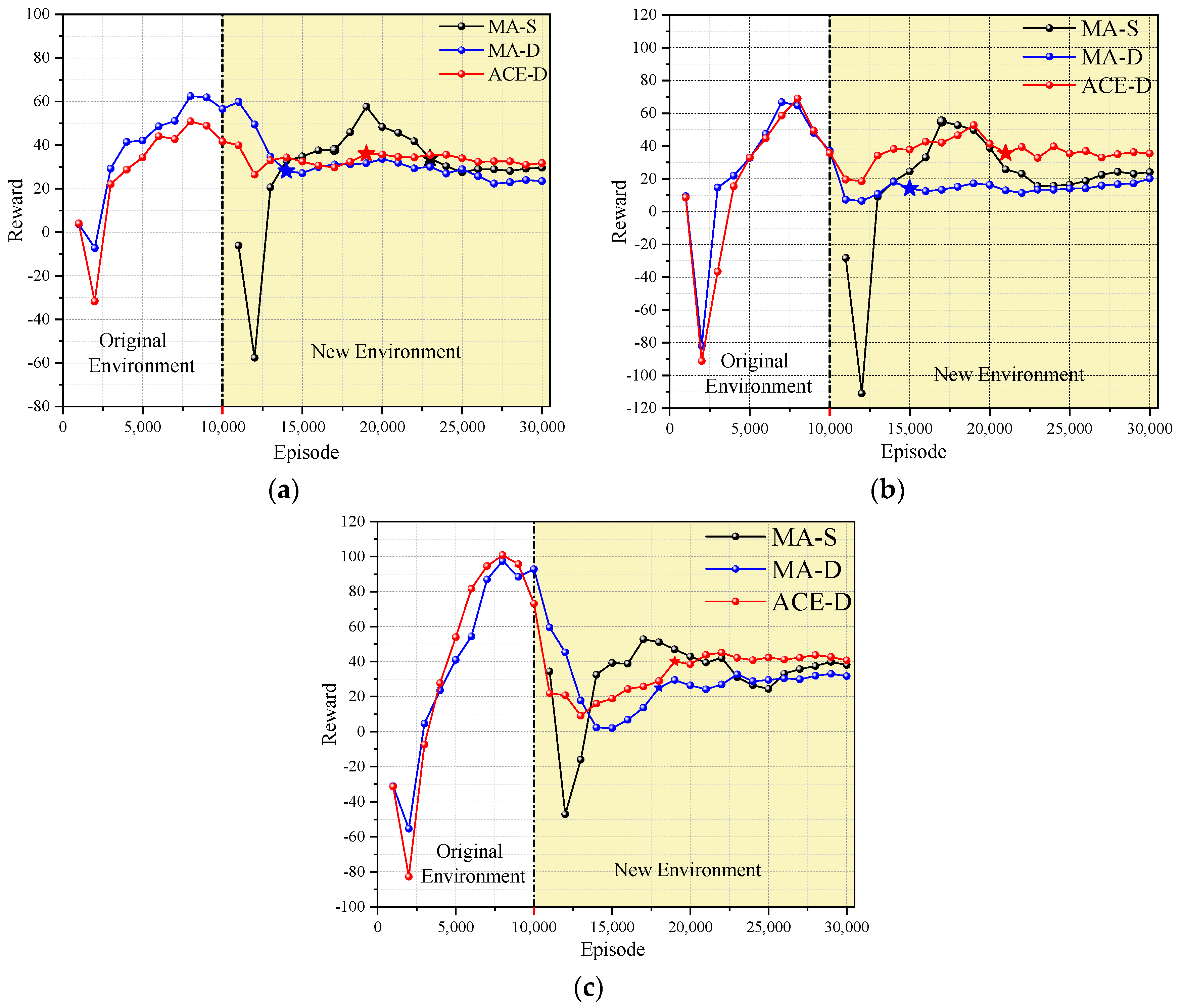
In order to evaluate the multi-agent adaptive co-evolutionary method in dynamic environment (ACE-D) proposed in this paper, three sets of dynamic environments are built for experiments based on MPE scenario and python3.8. Among them, Section 4.1 is about the ablation experiments, to investigate the effects of the experience screening policy (ES), adaptive weighting policy (AW), and ACE-D method separately in a simple pursuit scene; Section 4.2 is about the composite dynamic environment experiments, to verify whether the ACE-D method is still effective when environment change to a more complex and composite situation within which the initial position of the obstacles and the agents vary at different levels; Section 4.3 is about the continuously changing dynamic environment experiments, in which the environment changing happens more than once, to verify whether the ACE-D method is still effective when facing dynamically changing environments.

In this paper, the experiment uses Ubuntu20.04; the initial parameters ${\theta }^u$, ${\theta }^Q$ are all set to 0.5.

The algorithm MADDPG is taken for comparison, and when facing environment changing, two training modes are alternative for multi-agent co-evolution. One is to retrain the agents using the new environment information, denoted as MA-S; the second is to continue the training on the basis of the model trained in the previous environment, denoted as MA-D. Our ACE-D is designed special for dealing with the dynamic changes of the environment and therefore faces no choice to retrain or retain.

Recall that the purpose of multi-agent co-evolution is to achieve high efficiency while achieving maximum rewards. Therefore, this paper evaluates the co-evolution effect by checking the reward value and convergence efficiency in a stable state. It has to remind one that facing dynamic environments, the local optimum would appear in the experiment. If it falls into the local optimum, the multi-agent will converge to an abnormal stable state. It is meaningless to compare the convergence efficiency; in this case, only the reward is used as an effective index. If it does not fall into local optimum, the reward growth rate and convergence efficiency growth rate are used as evaluation indicators.

Local optima definitely impact the performance of the algorithms; thus, it is recommend to be considered as an influencing factor. Considering the influence of the dynamic environment, the parameter $\sigma$ is designed to represent the degree of local optimum as shown in Equation (16):

$$\sigma =\frac{R-r^{″}}{r^{″}}$$

(16)

where $r^{″}$ is the average reward of MADDPG by retraining towards a stable state in a static new environment (MA-S), and $R$ is the average stable reward of other different methods used in the experiment to deal with dynamic environment. The local optimal degree $\sigma$ is based on $r^{″}$ and represents the degree of difference between different methods and MA-S. If $\sigma \le \tau$, it is considered to be trapped in local optimum, where $\tau$ is a constant and set to be $\tau =-0.2$.

The other experimental parameters and meanings are shown in

Table 2. Experimental parameters in dynamic environment.

Parameters	$\mathit{r}$	${\mathit{r}}^{\prime }$	$\mathit{k}$	${\mathit{k}}^{\prime }$
Meaning	Stable rewards of MADDPG	Stable rewards of ACE-D	Number of MADDPG training	Number of ACE-D training
Parameters	${\mathit{\phi }}^{\prime }$	${\mathit{\phi }}^{″}$	$\mathit{\sigma }$
Meaning	Rewards growth rate ${\phi }^{\prime }=\frac{r^{\prime }-r}{r}$	Efficiency growth rate ${\phi }^{″}=\frac{k-k^{\prime }}{k}$	Local optimal degree $\sigma =\frac{R-r^{″}}{r^{″}}$

:

4.1. Ablation Experiments

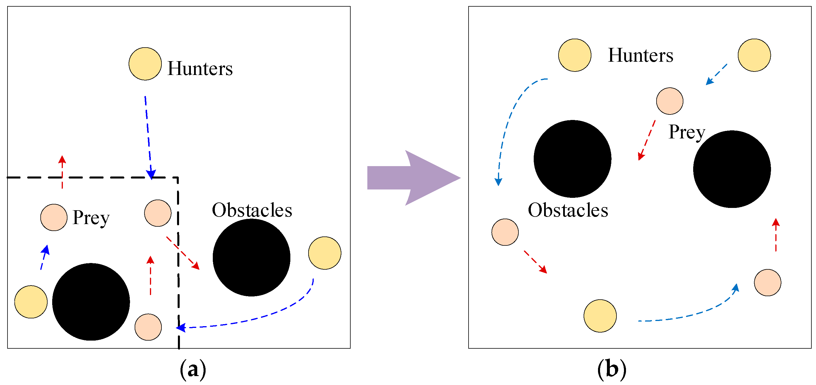
The ablation experiments are designed as shown in Figure 3; there are three hunters, three prey, and two obstacles in this experimental scene. The hunters are rewarded by shortening the distance between them and the prey as well as capturing the prey, while the prey will move away from the hunters to obtain the reward.

The experiment trains 30,000 episodes; each episode includes 25 iterations. The initial positions of hunters and obstacles are randomly generated in the environment, while the initial positions of prey change over time. In the first 10,000 episodes, the training environment is as shown in Figure 3a. The initial position of the prey is fixed in the inner area of the dotted box in the lower left corner of the scene. Then, the environment changes to the new environment shown in Figure 3b, and the initial position of the prey is randomly generated in the whole map.

As shown in Figure 3, the environment changes from the original environment to the new environment. Five methods are used for learning, which are MA-D, experience screening policy (ES), adaptive weighting policy (AW), MA-S, and ACE-D. Comparisons about their effects are carried out as ES vs. MA-D, AW vs. MA-D, ACE-D vs. MA-D, and ACE-D vs. MA-S. The results are shown in Figure 4 and

Table 3. Ablation experiment results.

Method	Average Stable Rewards	$\mathit{\sigma }$	Local Optimal	Number of Training (k)	Rewards Growth Rate (%)	Efficiency Growth Rate (%)
MA-S	31.28	0	No	13	32.32	−85.71
MA-D	23.64	−0.244	Yes	7	0	0
ES	26.46	−0.154	No	9	8.5	−28.6
AW	29.48	−0.058	No	16	24.7	−128.6
ACE-D	29.56	−0.055	No	6	25	14.3

:

It can be seen from Figure 4 that the average stability rewards of the AW policy, ES policy, and ACE-D method are higher than those of MA-D, and the training efficiency of the ACE-D method is higher than that of MA-S. As can be seen from Table 3, the local optimum degree $\sigma$ of MA-D in a dynamic environment is −0.244, indicating that MA-D is trapped in local optimum, while the ES policy, AW policy, and ACE-D method proposed in this paper avoid the local optimum as expected. In the ablation experiment, the average stable reward of the ACE-D method is close to that of the MA-S method, and the training efficiency of the ACE-D method is 30.77% higher than that of the MA-S method, which indicates that the ACE-D method is more efficient in dealing with the dynamic environment than the MA-S method.

In addition, in terms of stable rewards, the ACE-D method is 25% higher than the MA-D method, which is close to the 24.7% that contributed by the AW policy while the ES promotes only 8.5% comparing with the MA-D, separately. It implies that the AW policy plays a major role in getting rid of the local optimum. The convergence efficiency of the ES policy and the ACE-D method is 43.75% and 62.5% higher than that of the AW policy, respectively, indicating that the main role of the ES policy is to improve the training efficiency. The experimental results show that the ACE-D method combines the advantages of the ES policy and the AW policy and has the ability to get rid of the local optimum and reach the stable state in the new environment faster, so as to realize the co-evolution of multi-agent in the dynamic environment.

4.2. Composite Dynamic Environment Experiment

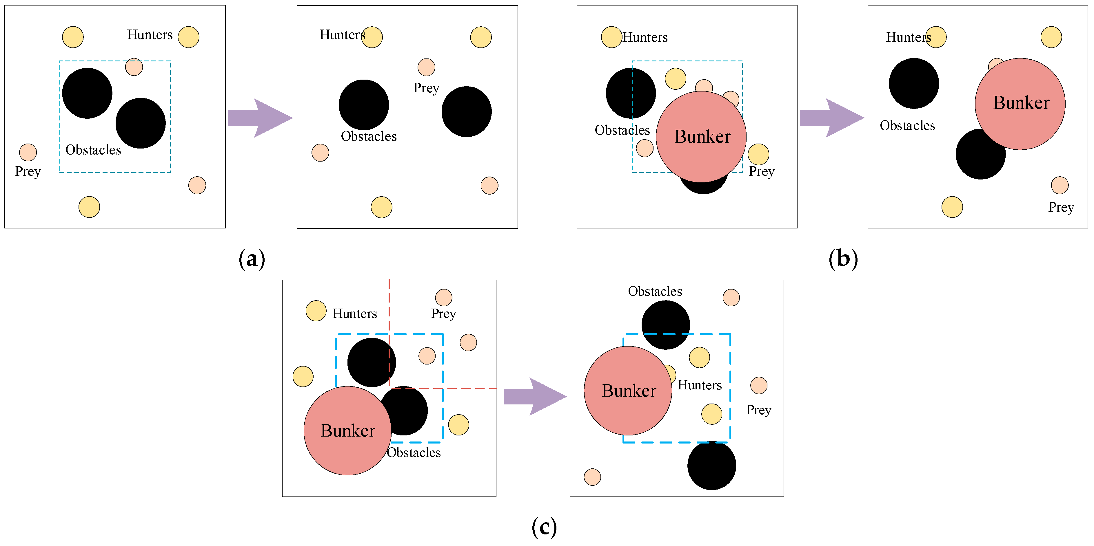
In order to verify the effectiveness of the ACE-D method under compound dynamics, three sets of dynamic scenarios with increasing complexity are designed in this section. Scenario 1 is a dynamic environment with the initial position change of obstacles, as shown in Figure 5a; the initial positions of obstacles in the original environment are restricted within the dashed box, and the positions are random after the environment change; scenario 2 is a dynamic environment with the initial position change of agents, as shown in Figure 5b; compared with Scenario 1, a red bunker is added to the environment, and when there is an agent into the bunder, the rest of agents cannot get its information. Positions of prey in the original environment are restricted to the dashed box, and the positions of the agents and the obstacles are random after the environment changes; scenario 3 is a dynamic environment compounded by the previous two basic dynamic environments, as shown in Figure 5c; in the original environment, the positions of obstacles are restricted to the blue dashed box, and the positions of prey are restricted to the red dashed box. After the environment changes, the initial position of the hunters is restricted to the blue dashed box, and the rest of the positions are random. The results are shown in Figure 6 and

Table 4. Comparison of training results of three sets of complex dynamic scenarios.

Scenario	Method	Average Stable Rewards	$\mathit{\sigma }$	Local Optimal	Number of Training (k)	Rewards Growth Rate (%)	Efficiency Growth Rate (%)
Scenario 1	MA-S	31.28	0	No	13	34.89	−225
	MA-D	23.19	−0.259	Yes	4	0	0
	ACE-D	30.77	−0.016	No	8	32.69	−100
Scenario 2	MA-S	33.9	0	No	21	122.6	−320
	MA-D	15.23	−0.551	Yes	5	0	0
	ACE-D	35.98	0.061	No	11	136.2	−120
Scenario 3	MA-S	43.22	0	No	22	44.69	−175
	MA-D	29.87	−0.309	Yes	8	0	0
	ACE-D	41.93	−0.03	No	9	40.37	−12.5

:

As can be seen from Figure 6, both MA-D and ACE-D converge faster after dynamic changes in the environment; the convergence efficiency of MA-S is much lower than the other two methods, but MA-D has the lowest stable reward. As can be seen from Table 4, the local optimality $\sigma$ of MA-D in the three scenarios after dynamic environment changes is −0.259, −0.551, and −0.309, respectively, which indicates that the MA-D method falls into local optimality in all three scenarios, indicating that MA-D has a poor ability to cope with the dynamic environment.

In all three scenarios, the stable rewards of ACE-D method and MA-S are very close, but the convergence efficiency of ACE-D method is improved by 38.5%, 47.6%, and 59.1%, respectively, compared with MA-S. As the complexity of the environment increases, the number of training sessions consumed by MA-S gradually grows, while the ACE-D method can use the training results of the original environment and has a significant advantage in the efficiency of adapting to the new environment compared with MA-S. The results demonstrate that the ACE-D method could achieve co-evolution in complex dynamic environments successfully. It also seems that the more complex the environment is, the more obvious the advantage of the ACE-D method is.

4.3. Continuously Changing Dynamic Environment Experiment

Most of the dynamic changes of the real environment happen more than once, and are unpredictable in time, so two sets of continuously changing scenarios are designed in this group of experiments shown in Figure 7, which has three prey, three hunters, and two obstacles. The training is carried out in total of 60,000 episodes, and the original environment is shown in Figure 7a.

The time intervals between the two dynamic changes of the environment in the two sets of scenarios are different. In continuous change scenario 1, the first change of the environment occurred around the 10,000 episodes when the multi-agent had not reached a stable state yet. The second change happened around the 35,000 episodes, when it had reached a stable state; in continuous change scenario 2, the first change was at the 30,000 episodes, when the multi-agent reached a stable state, and the second change was at the 40,000 episodes, when it had not adapted to the new environment yet. The experimental results are shown in

Table 5. Comparison of training results for continuous change scenario 1.

Environment	Method	Average Stable Rewards	$\mathit{\sigma }$	Local Optimal	Number of Training (k)	Rewards Growth Rate (%)	Efficiency Growth Rate (%)
The First Change	MA-S	32.08	0	No	18	32.51	−157.1
	MA-D	24.21	−0.245	Yes	7	0	0
	ACE-D	35.01	0.091	No	9	44.61	−28.57
The Second Change	MA-S	31.28	0	No	13	31.48	−160
	MA-D	23.79	−0.239	Yes	5	0	0
	ACE-D	33.54	0.072	No	10	40.98	−100

and

Table 6. Comparison of training results for continuous change scenario 2.

Environment	Method	Average Stable Rewards	$\mathit{\sigma }$	Local Optimal	Number of Training (k)	Rewards Growth Rate (%)	Efficiency Growth Rate (%)
Original	MA-D	31.27	0	No	20	0	0
	ACE-D	31.56	0.009	No	20	0.01	0
The Second Change	MA-S	31.28	0	No	13	34.71	−160
	MA-D	23.22	−0.258	Yes	5	0	0
	ACE-D	30.37	−0.032	No	9	30.79	−80

.

From Figure 8 and Figure 9, it can be seen that in the case of continuous changes in the environment, the ACE-D method can respond to the changes in the environment quickly and adapt to the new environment regardless of when the dynamic environment changes occur, while MA-D is more likely to fall into the local optimum. As can be seen from Figure 9, MA-D responds when the environment changes at the first time, but the response speed is lower than that of ACE-D method, and ACE-D method adapts to the new environment faster than MA-D; at the second environment change, MA-D almost loses its response function, and the reward does not appear to be significantly changed, but the ACE-D method is basically unaffected, from which it can be seen that multiple changes of the environment can aggravate the local optimum and hinder the co-evolution.

From Table 5 and Table 6, we can learn that after the change of environment, the local optimality $\sigma$ of MA-D is −0.245, −0.239, and −0.258, which are all smaller than $\tau$; that is, MA-D falls into the local optimum. After the secondary change of the environment, the stable rewards of ACE-D method and MA-S method are improved by more than 30% compared with MA-D, but the ACE-D method is more efficient compared with MA-S, and the improvement is above 23%, which proves that the continuous change of the environment does not affect the ability of ACE-D method to cope with the dynamic environment. The comparison results show that the ACE-D method is largely unperturbed by continuous changes in the environment and is able to respond to environmental changes rapidly and achieve co-evolution in the continuously changing dynamic environment.

5. Conclusions

A multi-agent adaptive co-evolution method in dynamic environments is proposed in this paper, which gradually adjusts the environment exploration policy to an optimal policy that adapts to the new environment when the environment changes dynamically while avoiding falling into a local optimum and achieving co-evolution of a multi-agent. The proposed ACE-D method can be applied to various multi-agent decision-making scenarios in dynamic environments, such as cooperative UAV missions, swarm robots, and group gaming games, providing a feasible approach to solve the problem of multi-agent systems easily falling into overfitting in dynamic environments. The ACE-D method consists of the experience screening policy and the adaptive weighting policy. The experience screening policy separates the experiences of different environments, retains the favorable experiences of the original environment while excluding the unfavorable effects, and focuses on adapting to the new environment. The experience screening policy improves the training efficiency by 30.8% over MA-S and the stable reward by 8.5% over MA-D, which indicates its efforts for a multi-agent to adapt to new environments. The adaptive weighting policy prioritizes learning by assigning high weights to the actions that are more rewarding and beneficial for agent co-evolution in the new environment and improves the stable reward by 24.7% over MA-D to avoid falling into the local optimum. The ACE-D method combines the above two policies and is validated in different classes and dynamic environment tasks of different complexity. The ACE-D method cannot only cope with various dynamic environments and avoid local optimums but also make a big improvement in the speed of adapting to new environments, and the more complex the dynamic environment is, the more obvious the advantage of the ACE-D method is. The experimental results demonstrate that the ACE-D method can achieve the co-evolution of a multi-agent in various dynamic environments. Our future work will focus on dynamically changing detection and more complex dynamic environments.