Abstract
In this paper, we studied single-server models of queuing-inventory systems (QIS) with catastrophes in the warehouse part and negative customers (n-customers) in service facility. Consumer customers (c-customers) that arrived to buy inventory can be queued in an infinite buffer. Under catastrophes, all inventory of the system is destroyed but customers in the system (on server or in buffer) are still waiting for replenishment of stocks. Upon arrival of n-customer one c-customer is pushed out, if any. One of two replenishment policies (RP) can be used in the system: either or randomized. In the investigated QISs, a hybrid service scheme was used: if upon arrival of the c-customer, the inventory level is zero, then according to the Bernoulli scheme, this customer is either lost (lost sale scheme) or joining the queue (backorder scheme). Mathematical models of the investigated QISs were constructed as two-dimensional Markov chains (2D MC). Ergodicity conditions of the investigated QISs were obtained, and the matrix-analytic method (MAM) was used to calculate the steady-state probabilities of the constructed 2D MCs. Formulas for performance measures were found and the results of numerical experiments are presented.
MSC:
60J28; 60K25; 90B05; 90B22
1. Introduction
Queuing systems (QS), in which to service the customer, along with an idle server, certain items are also required, are called queuing-inventory systems (QIS), see [1,2]. In other words, QISs simultaneously possess the properties of classical QS and inventory control systems (ICS). In classical QS, only an idle server is enough to service a customer (in multi-rate QS, several idle servers will be required at the same time), and in classical ICS, the inventory is released to customers instantly, i.e., in classical ICS, there are no servers for customer service. However, in many real ICS, delivery of the inventory to customers is carried out using certain devices (servers), and this process will require some positive time to complete. Since the flow of customers is a random one, and the service time (i.e., the process of issuing stocks to customers) is a random variable, a queue of customers is formed to receive stocks. In other words, in QISs, it is necessary to manage both service and inventory control processes simultaneously, i.e., it is necessary to organize the process of servicing of customers and manage the inventory of the system.
The first work devoted to the study of QISs models are the works [3,4]. After these works, models of QISs were intensively studied by various authors over the past three decades. A detailed overview of known results is set out in the work [5].
In each QIS model, it is necessary to make certain assumptions about the type of distribution functions (d.f.) of random variables that form the model under study, i.e., d.f. of input flow, service time, the lifetime of inventory, etc. In addition, it is necessary to define the replenishment policy (RP) used. Usually, this d.f. and RP are the basis for classifying of QISs models. Based on the purpose of the considered paper, here, we will use the classification of QISs based on the lifetime of the stocks. According to this indicator, all QISs can be divided into two classes: QISs with an infinite life of stocks (i.e., the stocks of the system never deteriorate) and QISs with a finite life of stocks (i.e., the stocks of the system deteriorate after a finite time). Models of QISs with an infinite life of stocks are studied in detail in the available literature, see [5].
In models of perishable QISs, stock deterioration occurs within a certain positive time interval. In the class of perishable QISs, two sub-classes of systems are distinguished: (1) QIS with individual lifetime (ILT) in which each item can perish independently of the others, and (2) QIS with common lifetime (CLT) where all items perish together, e.g., foods with the same expiry date, medicines manufactured with the same expiry date and so on. Note that models of perishable QIS with ILT were intensively investigated, see, e.g., [6,7,8,9] and their reference lists. However, models of perishable QIS with CLT were little studied, see [10,11,12,13].
It is important to note that, in practice, there are QISs in which items can be destroyed instantly due to various reasons, e.g., due to the negligence of warehouse workers, as a result of a sudden power outage, etc. Despite their importance, such models of QISs were hardly studied, see [14,15,16,17]. Note that in the indicated papers, it was assumed that upon accident, the inventory level was instantly reduced only by one. In the present work, QIS models with catastrophes in the warehouse part of the system are studied. This means that all stocks of the system are destroyed at the same time. At first glance, it may seem that the models of QISs with catastrophes are similar to models of QISs with CLT, but these models differ from each other. Indeed, in models of QISs with CLT, it is required that, at any given time, all stocks in the warehouse have the same age, i.e., it is considered that all stocks arrived as a result of execution of one batch of orders. One can be achieved as follows: any items remaining in the inventory at the time of replenishment will be removed to accommodate the new batch of items, where is a maximum inventory capacity, see [10]. However, in the model of QIS with catastrophe, this rather rigid assumption is removed.
Note that the classical models of QS with catastrophes were studied in detail in the available literature, see [18,19,20,21,22,23,24]. These papers considered that, as a result of a catastrophe, the servers of the system fail, while the customers are not affected and they are waiting for the servers to be repaired. In other words, QS models with catastrophes are a useful tool for studying systems with unreliable servers.
Another feature of the QIS models studied here is that in addition to consumer customers, c-customers (i.e., customers that arrived to purchase the inventory), negative customers (n-customers) also enter the system. Negative customers do not require the stocks, but they force one C-customer out of the system. At the same time, n-customers will not affect the stocks of the system. For more details about the QS with n-customers, readers can refer to the pioneering work [25], as well as the review paper [26].
Despite their importance, QIS models with n-consumers almost were not studied in the available literature. To the best of our knowledge, for the first time, the Markovian model of single-server perishable QIS with finite waiting room under (s,Q), Q = S − s > s + 1, replenishment policy was considered in [27]. It is assumed that both types of customers, consumer and negative, arrive according to a Markovian arrival process (MAP). Authors considered the following removal rule: an n-customer at an arrival epoch removes one or more waiting c-customers and the number of removals is a random variable depending on the number of waiting c-customers in the system. The joint probability distribution of the number of c-customers in the system and the inventory level is obtained and various performance measures of the system are computed as well as the total expected cost rate is calculated. This paper showed also examples of real-life situations in which QIS models with n-customers can be applied. For instance, some people who promote the goods of other sellers may advertise their goods among the customers of this system, and thus, the customers of this system may leave the system without receiving its goods. In a recent paper [28], n-customers were taken into account for the perishable QIS model with double sources for replenishments.
Note that catastrophes and n-customers make models of QIS more realistic. To our best knowledge, no existing works on QIS management considered these two features simultaneously. It was also unclear whether known RPs still work well in this setting. As a result, it is desirable to develop models of such QISs and deeply analyze this problem. On the other hand, considering these realistic features simultaneously increases the difficulty of the constructed mathematical models as well as their computational complexity. The considered work is the first attempt in this direction.
Most of the existing literature on the QIS assumed that one of the following schemes is applied: (i) lost sales where any customer that faces a zero inventory is lost or (ii) backorder sales where each customer joins the queue if upon its arrival there is no inventory. However, in real QISs, some customers may join the queue or be lost according to the Bernoulli scheme if the inventory level is zero at the time of their arrival. We will call these schemes hybrid sales. Note that, to the best of our knowledge, QIS models with hybrid sales were hardly studied.
The next step after the description of the model was the choice of the appropriate mathematical tool. In this regard, we note that the matrix-analytic method (MAM) [29] is an effective tool. A modern exposition of the basis of the theory and practice of MAM can be found in monographs [30,31,32,33,34].
An analysis of the available literature showed that they studied QIS models under several unrealistic assumptions. For instance, in known works, it was assumed that, in the warehouse, there were no accidents that lead to the destruction of the entire inventory and the system used a unique sales scheme. In addition, most known works did not take into account the possibility of negative customers. Therefore, we summarize the main contributions of this work as follows:
- Our model simultaneously captures three important and realistic features of QISs: catastrophes in a warehouse, negative customers in a service facility, and hybrid sales;
- The investigated QISs can operate under two RPs: policy or randomized replenishment policy;
- We obtain the easily checkable stability conditions of the investigated systems and show that in special cases, they do not depend on the storage size, the rate of catastrophes as well as the replenishment rate;
- Simple formulas for steady-state probability vectors as well as for performance measures of our systems are developed;
- The developed formulas allow analyzing of the effect of the initial parameters on performance measures of the studied QISs as well as on expected total cost (ETC) and appropriately select the optimal RPs parameters so that the ETC is minimized.
This paper is organized as follows. In Section 2, we describe the QIS models, clarifying the assumptions of the d.f. random variables that form the models. Stability conditions for both models are established and MAM is used for steady-state analysis of the models are given in Section 3. Explicit formulas for key performance measures are obtained in Section 4. The results of numerical examples are shown in Section 5. Concluding remarks are given in Section 6.
2. Describing the Models
The block diagram of the investigated single-server QIS of infinite capacity is shown in Figure 1. The homogeneous c-customers arrive at the service facility according to Poisson process with rate . The service times of the c-customers are assumed to be exponentially distributed with parameter . The service requires an idle server along with items (one for each c-customer) that are stored in an inventory of maximum capacity S.
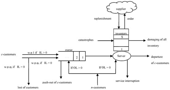
Figure 1.
Block diagram of the system under study.
In the system, hybrid sales scheme is used, i.e., some part of c-customers is serviced according to the backorder sale scheme, while the other part is serviced according to the lost sale scheme. This means the following: if there are no stocks in the system upon arrival of c-customer, then, in accordance to the Bernoulli trials, it either, with probability (w.p.), joins the queue of infinite length (backorder sale scheme), or w.p. leaves the system unserved (lost sale scheme), where .
The system also receives n-customers with a rate When a n-customer arrives, one c-customer force out of the system. A n-customer can force out of the system even a c-customer, which is in the server, while the inventory level does not change, since it is assumed that stocks are released after the completion of servicing a c-customer. If there is a queue of c-customers at the time an n-customer arrives, then only the c-customer is pushed out from the queue (i.e., the service of the c-customer, which is in the server, continues); if there are no c-customers in the system, then the received n-customer does not affect the operation of the system.
In the system, catastrophic events can occur only in its warehouse part. The flow of catastrophic events is Poisson one with the parameter , and at the moment of arrival of such an event, all the reserves of the system are instantly destroyed. As a result of the catastrophes, even the stock, which is at the status of release to the c-customer, is destroyed. In the latter case, the c-customer whose service was interrupted due to a catastrophe is returned to the queue; in other words, the catastrophe only destroys the stocks of the system and does not force c-customers out of the system. If the inventory level is zero, then the disaster does not affect the operation of the system warehouse.
Here, two inventory replenishment policies were considered. The first RP was according to a -type policy (sometimes this policy is called “Up to S”). In this policy, when the inventory level drops to the reorder point where an order was placed for replenishment and upon replenishment, the inventory level was restocked to level S, no matter how many items are still present in the inventory. Second RP is randomized (randomized replenishment policy, RRP), see [35]. In RRP, an order is placed only when the system’s warehouse is completely empty and the volume of the supplied stock is a random variable with a known distribution; in other words, w.p. , the volume of incoming stock is equal to , where . In both RPs, the parameter indicates the reorder rate per order.
The task is to find the joint distribution of the number of c-customers in the system and the inventory level of the system, as well as to calculate the key performance measures of the system.
3. Stationary Distributions
First consider the computation of the steady-state probabilities of the system under policy. Let be the number of customers at time and be the inventory level at time . Then, the process forms a continuous time Markov chain (CTMC) with state space
where is the subset of state space with called the level .
Let denote the transition rate from state to state So, by noting the assumptions made in Section 2, we conclude that the investigated CTMC has a generator with the following transition rates for
Hereinafter, is the indicator function of the event , which is 1 if is true and 0 otherwise.
By re-numbering the states of the system in a lexicographic way, from relations (1)–(6) we conclude that the process is a level independent quasi birth–death (LIQBD) process and its generator might be represented as follows:
where O denotes zero square matrix with dimension and all other block matrices are square matrices of the same dimension. Entities of the block matrices and are determined as follows:
The entities of the generator are determined as follows:
The stationary probability vector that corresponds to the generator is denoted by . In other words, we have the balance equations:
where 0 is the null row vector of dimension S + 1 and e is the column vector of dimension S + 1 that contains only 1’s.
By using the recursive procedure, we obtained that Equation (13) had the following solution:
where ,
Using the stationary probability vector of the generator given by (14), we can derive the ergodicity (stability) condition of the process .
Proposition 1.
Under policy, the processis ergodic if and only if the following condition is fulfilled:
Proof of Proposition 1.
In accordance with [29] (pp. 81–83), the process is ergodic if and only if
By using relations (14), from the matrices and , we have
and
Thus, relation (16) is equivalent to the inequality (15). □
Note 1.
The established ergodicity condition (15) has a probabilistic meaning, i.e., it indicates that the rate of c-customers entering the system must be less than the total rate of negative customers and the rate of served c-customers. We find from (15) that in general case stability condition for the present model is dependent on the storage size of system, the rate of catastrophes, and the replenishment rate.
Note 2.
Consider the following special cases.
(i) If (i.e., when a pure lost sale scheme is used) and (i.e., when there are not negative customers) from (9), we find the ergodicity condition for the single-server Markovian queuing system, i.e., . In other words, under such assumptions, the ergodicity condition of the system does not depend on the storage size of system, the rate of catastrophes, and the replenishment rate. Similar results for other models were obtained in [9,36,37].
(ii) If and , the ergodicity condition is depending on all indicated parameters of the system, see Formula (14).
(iii) If (pure backorder scheme is used), the ergodicity condition is dependent on all indicated parameters of the system even for case , see Formula (14).
A steady-state probability that corresponds to the generator matrix , we denote by , where . Under the ergodicity condition (15), desired steady-state probabilities are determined from the following equations:
where R is the nonnegative minimal solution of the following quadratic matrix equation:
From (8)–(11), it was concluded that bound probabilities are determined from the following system of equations with normalizing conditions:
where I indicate the identity matrix of dimension .
Now consider the computation of the steady-state probabilities under RRP. In this case, parameters are calculated via relations (1)–(5) but relation (6) should be substituted by the following equations:
where
Therefore, for this policy the generator matrix of the process has the following form:
Here, entities of matrices and are calculated as follows:
In this model, entities of the generator are determined as
Again, using the recursive procedure, we found that the balance Equation (13), where the matrix is replaced by , the following solution was used
where are calculated from the following reverse recursive relations
Here, the unknown parameter is found from the normalizing condition, i.e.,
In analogy with Proposition 1, it is easy to show that the following fact is true.
Proposition 2.
Under RRP policy, the process is ergodic if and only if the condition (15) is fulfilled where is defined as in (23).
Furthermore, by using a system of Equations (17) and (18), the steady-state probabilities for this model were calculated.
4. Performance Measures
In this section, we are interested in the key performance measures of the investigated system related to both inventory and queuing under each RP. Having determined the steady-state probabilities under both RPs, we can compute the key performance measures of the investigated models explicitly.
Performance measures related to inventory are the following:
- Average inventory level under both policy
- Average order sizeunder policyunder RRP
- Average reorder rateunder policyunder RRP
Performance measures related to queuing are the following:
- Average length of the queue under both policies
- Loss rate of customers under both policies
5. Numerical Results
Here, we consider the results of numerical experiments for both models. These experiments were generated using a Fortran 90 code due to the authors’ years of experience with this software. The running time (i.e., time from compiling the program to the time results appear) was only a few seconds.
Below, hypothetical models were considered for both policies, i.e., the values of initial parameters were chosen arbitrarily. Note that in realistic applications, these values can be changed.
First, consider the results for the model with “Up to ” policy. For this RP, we considered the behavior of performance measures versus as well as the finding the optimal value of to minimize the expected total cost (ETC) that was defined as follows:
where is the fixed price of one order, is the unit price of the order size, is the unit inventory storage price per unit of time, is the price of unit inventory damaging, is the cost for a single c-customer loss, is the price per unit time of queuing delay for a single c-customer.
For this policy, it was assumed that values of all parameters of the QIS were fixed except the parameter . In other words, here, numerical experiments were processed to analyze the effect of parameter on the performance measures.
Let us consider and that values of load parameters are selected as follows: . The coefficients in the expression for functional in ETC (see (31)) were chosen as follows: .
The impact of reorder points on performance measures, ETC, are shown in Table 1. From this table, we conclude that the rate of change of all performance measures was very low and ETC was a unimodal function; its minimal value is indicated in bold.

Table 1.
Impact of reorder point to performance measures and ETC.
The goals of the numerical experiments for the model with RRP were the investigation of the behavior of performance measures versus initial parameters for three schemas of changing of probabilities : (1) when are constants, (2) when are increasing ones, and (3) when are decreasing ones.
Here, we again assumed that and . Additionally, in the first schema, we set in the second schema, we set in the third schema, we set
Values of other parameters are shown in the title of the appropriate Table 2, Table 3, Table 4 and Table 5. In these tables, the first row corresponds to schema (1), the second row corresponds to schema (2), and the third row corresponds to schema (3).
Table 2.
Performance measures vs. under RRP, .
Table 3.
Performance measures vs. under RRP; .
Table 4.
Performance measures vs. under RRP; .
Table 5.
Performance measures vs. under RRP; .
Now, we present the effect of initial parameters as well as considered schemas of changing probabilities on the performance measures of the investigated RRP as follows:
- An analysis of data in Table 2, Table 3, Table 4 and Table 5 showed that the second schema was favorable for all performance measures, except for the average inventory level. For the average inventory level, the third schema was favorable. It is interesting to note that the first schema was always intermediate between the three schemes.
- Table 2 shows that for all schemas, except for the average inventory level, performance measures increased versus the rate of consumer customers. These findings were expected.
- From Table 3, we can see that the average inventory level as well as the rate of loss of consumer customers increased when the rate of negative customers increased. However, the main performance measures decreased as the rate of negative customers increased. These findings were true for all schemas, and they were also expected.
- From Table 4, we can notice that the average inventory level as well as the reorder rate increased when the replenishment rate increased. A first observation concerning the behavior of reorder rate was unexpected. This phenomenon was explained as follows: when the replenishment rate increased, the probability that the inventory level was positive also increased and, hence, the catastrophe rate increased (see the second term in Formula (28)). Here, the rest of the performance measures were decreased versus replenishment rate. These findings were true for all schemas, and they were also expected.
- Table 5 shows that for all schemas, excluding the average inventory level, performance measures increased versus the rate of catastrophes. These findings were true for all schemas, and they were also expected.
6. Conclusions
A new model of the single-server QIS with negative customers and catastrophes in the warehouse under two replenishment policies was proposed. One of the replenishment policies was “Up to S” and the other was a randomized policy. The combination of lost sale scheme and backorder scheme was used, i.e., if the inventory level upon arrival of consumer customer was zero, then, in accordance to the Bernoulli trials, it either joined the queue of infinite length (backorder sale scheme), or left the system unserved (lost sale scheme). Negative customers required neither service nor inventory, i.e., upon the arrival of such a customer, one of the consumer customers was pushed out of the system. In the case of a catastrophe, all items in the warehouse, as well as items that were at the status of release to the consumer customer, were instantly destroyed but catastrophes did not force the consumer customers out of the system.
The mathematical models of the investigated system under both policies were two-dimensional Markov chains with different three-diagonal generators. The ergodicity conditions for the constructed 2D MC were found and probabilistic means of the obtained conditions were given. It was shown that some known results were special cases of the developed conditions. Formulas for calculating the performance measures were proposed. The results of numerical experiments were analyzed.
The direction of future work should be the investigation of the models with MAP flows of c-customers and/or n-customers as well as with PH distribution of service times for c-customers.
Author Contributions
Conceptualization, A.M.; methodology, A.M. and J.S.; software, L.P. and S.E.; investigation, A.M., J.S., L.P. and S.E.; writing—review and editing, A.M., J.S., L.P. and S.E.; supervision and project administration, A.M. All authors have read and agreed to the published version of the manuscript.
Funding
This research received no external funding.
Institutional Review Board Statement
Not applicable.
Informed Consent Statement
Not applicable.
Data Availability Statement
Not applicable.
Conflicts of Interest
The authors declare no conflict of interest.
List of Acronyms
| ETC | Expected Total Cost |
| ICS | Inventory Control System |
| ILT | Individual Life Time |
| CLT | Common Life Time |
| MAM | Matrix-Analytic Method |
| MAP | Markovian Arrival Process |
| QS | Queuing System |
| QIS | Queuing-Inventory System |
| RP | Replenishment Policy |
| RRP | Randomized Replenishment Policy |
| IL | Inventory Level |
| QL | Queue Level |
References
- Schwarz, M.; Daduna, H. Queuing Systems with Inventory Management with Random Lead Times and with Backordering. Math. Methods Oper. Res. 2006, 64, 383–414. [Google Scholar] [CrossRef]
- Schwarz, M.; Sauer, C.; Daduna, H.; Kulik, R.; Szekli, R. M/M/1 Queuing Systems with Inventory. Queuing Syst. Theory Appl. 2006, 54, 55–78. [Google Scholar] [CrossRef]
- Melikov, A.; Molchanov, A. Stock Optimization in Transport/Storage Systems. Cybernetics 1992, 28, 484–487. [Google Scholar]
- Sigman, K.; Simchi-Levi, D. Light Traffic Heuristic for an M/G/1 Queue with Limited Inventory. Ann. Oper. Res. 1992, 40, 371–380. [Google Scholar] [CrossRef]
- Krishnamoorthy, A.; Shajin, D.; Narayanan, W. Inventory with Positive Service Time: A Survey, Advanced Trends in Queueing Theory; Series of Books “Mathematics and Statistics” Sciences. V., 2; Anisimov, V., Limnios, N., Eds.; ISTE & Wiley: London, UK, 2021; pp. 201–238. [Google Scholar]
- Hanukov, G. A queueing-inventory system in which customers can orbit during the service. IFAC Pap. 2022, 55, 619–624. [Google Scholar] [CrossRef]
- Ko, S.S. A Nonhomogeneous Quas-Birth Process Approach for an (s, S) Policy for a Perishable Inventory System with Retrial Demands. J. Ind. Manag. Opt. 2020, 16, 1415–1433. [Google Scholar] [CrossRef]
- Melikov, A.; Krishnamoorthy, A.; Shahmaliyev, M.O. Numerical Analysis and Long Run Total Cost Optimization of Perishable Queuing Inventory Systems with Delayed Feedback. Queuing Model. Serv. Manag. 2019, 2, 83–111. [Google Scholar]
- Melikov, A.; Shahmaliyev, M.; Nair, S.S. Matrix-Geometric Method to Study Queuing System with Perishable Inventory. Autom. Remote Control 2021, 82, 2168–2181. [Google Scholar] [CrossRef]
- Chakravarthy, S.R. An inventory system with Markovian demands, and phase-type distributions for perishability and replenishment. OPSEARCH 2010, 47, 266–283. [Google Scholar] [CrossRef]
- Krishnamoorthy, A.; Shajin, D.; Lakshmy, B. On a queueing-inventory with reservation, cancellation, common life time and retrial. Ann. Oper. Res. 2016, 247, 365–389. [Google Scholar] [CrossRef]
- Lian, Z.; Liu, L.; Neuts, F. A Discrete-Time Model for Common Lifetime Inventory Systems. Math. Oper. Res. 2005, 30, 718–732. [Google Scholar] [CrossRef]
- Shajin, D.; Krishnamoorthy, A.; Manikandan, R. On a Queueing-Inventory System with Common Life Time and Markovian Lead Time Process. Oper. Res. 2022, 22, 651–684. [Google Scholar] [CrossRef]
- Melikov, A.; Aliyeva, S.; Nair, S.; Krishna Kumar, B. Retrial queuing-inventory systems with delayed feedback and instantaneous damaging of items. Axioms 2022, 11, 241. [Google Scholar] [CrossRef]
- Melikov, A.; Mirzayev, R.R.; Nair, S.S. Numerical investigation of double source queuing-inventory systems with destructive customers. J. Comput. Syst. Sci. Int. 2022, 61, 581–598. [Google Scholar] [CrossRef]
- Melikov, A.; Mirzayev, R.R.; Nair, S.S. Double Sources Queuing-Inventory System with Hybrid Replenishment Policy. Mathematics 2022, 10, 2423. [Google Scholar] [CrossRef]
- Melikov, A.; Mirzayev, R.R.; Sztrik, J. Double Sources QIS with finite waiting room and destructible stocks. Mathematics 2023, 11, 226. [Google Scholar] [CrossRef]
- Demircioglu, M.; Bruneel, H.; Wittevrongel, S. Analysis of a Discrete-Time Queueing Model with Disasters. Mathematics 2021, 9, 3283. [Google Scholar] [CrossRef]
- Indra; Rajan, V. Indra; Rajan, VQueuing Analysis of Markovian Queue Having Two Heterogeneous Servers with Catastrophes using Matrix Geometric Technique. Int. J. Stat. Syst. 2017, 12, 205–212. [Google Scholar]
- Krishna Kumar, B.; Arivudainambi, D. Transient Solution of an M/M/1 Queue with Catastrophes. Comput. Math. Appl. 2000, 40, 1233–1240. [Google Scholar] [CrossRef]
- Sagayaraj, M.R.; Selvam, S.A.G.; Susainathan, R.R. An analysis of a queueing system with heterogeneous servers subject to catastrophes. Math. Aeterna 2015, 5, 605–613. [Google Scholar]
- Seenivasan, M.; Kameswari, M.; Chakravarthy, V.J.; Indumath, M. Analysis of queueing model with catastrophe and restoration. AIP Conf. Proc. 2021, 2364, 020034. [Google Scholar]
- Vinodhini, G.A.F.; Vidhya, V. Computational Analysis of Queues with Catastrophes in a Multiphase Random Environment. Math. Probl. Eng. 2016, 2917917. [Google Scholar] [CrossRef]
- Ye, J.; Liu, L.; Jiang, T. Analysis of a Single-Sever Queue with Disasters and Repairs under Bernoulli Vacation Schedule. J. Syst. Sci. Inf. 2016, 4, 547–559. [Google Scholar] [CrossRef]
- Gelenbe, E. Random Neural Networks with Positive and Negative Signals and Product Form Solution. Neural Comput. 1989, 1, 502–510. [Google Scholar] [CrossRef]
- Do, T.V. Bibliography on G-networks, Negative Customers and Applications. Math. Comput. Model. 2011, 53, 205–212. [Google Scholar] [CrossRef]
- Sivakumar, B.; Arivarignan, G. A Perishable Inventory System with Service Facilities and Negative Customers. Adv. Model. Optim. 2005, 7, 193–210. [Google Scholar]
- Soujanya, M.L.; Laxmi, P.V. Analysis on Dual Supply Inventory Model Having Negative Arrivals and Finite Lifetime Inventory. Reliab. Theory Appl. 2021, 16, 295–301. [Google Scholar]
- Neuts, M.F. Matrix-Geometric Solutions in Stochastic Models: An Algorithmic Approach; John Hopkins University Press: Baltimore, MD, USA, 1981. [Google Scholar]
- Chakravarthy, S.R. Introduction to Matrix-Analytic Methods in Queues; John Wiley & Sons, Inc.: London, UK, 2022; Volume 1. [Google Scholar]
- Chakravarthy, S.R. Introduction to Matrix-Analytic Methods in Queues; John Wiley & Sons, Inc.: London, UK, 2022; Volume 2. [Google Scholar]
- Dudin, A.N.; Klimenok, V.I.; Vishnevsky, V.M. The Theory of Queueing Systems with Correlated Flows; Springer Nature Switzerland AG: Basel, Switzerland, 2020. [Google Scholar]
- He, Q.-M. Fundamentals of Matrix-Analytic Methods; Springer: New York, NY, USA, 2014. [Google Scholar]
- Latouche, G.; Ramaswami, V. Introduction to Matrix Analytic Methods in Stochastic Modeling; SIAM: Philadelphia, PA, USA, 1999. [Google Scholar]
- Melikov, A.; Ponomarenko, L.; Bagirova, S. Models of queueing-inventory systems with randomized lead policy. J. Autom. Inf. Sci. 2016, 48, 23–35. [Google Scholar] [CrossRef]
- Krishnamoorthy, A.; Manikandan, R.; Lakshmy, B. Revisit to Queueing-inventory System with Positive Service Time. Ann. Oper. Res. 2015, 233, 221–236. [Google Scholar] [CrossRef]
- Zhang, Y.; Yue, D.; Yue, W. A Queueing-inventory System with Random Order Size Policy and Server Vacations. Ann. Oper. Res. 2022, 310, 595–620. [Google Scholar] [CrossRef]
Disclaimer/Publisher’s Note: The statements, opinions and data contained in all publications are solely those of the individual author(s) and contributor(s) and not of MDPI and/or the editor(s). MDPI and/or the editor(s) disclaim responsibility for any injury to people or property resulting from any ideas, methods, instructions or products referred to in the content. |
© 2023 by the authors. Licensee MDPI, Basel, Switzerland. This article is an open access article distributed under the terms and conditions of the Creative Commons Attribution (CC BY) license (https://creativecommons.org/licenses/by/4.0/).