Analysis of a Reaction–Diffusion–Advection Model with Various Allee Effects

Abstract

This paper presents an extensive study of traveling wave solutions for a population model where the growth function incorporates the Allee effect. We are able to find closed form solutions for solitary waves that are kinks and pulses (bell type). Additionally, for every solution that we find, we show the corresponding phase portrait. Interestingly, we discover that, under certain conditions, standing waves of the bell and kink types exist too.

1. Introduction

Over the years, it has become important to study population models with a variety of growth functions in order to understand a number of real world situations and make better predictions and management decisions [1]. Processes such as diffusion, reaction, advection, and the interactions between them should be taken into account when constructing realistic population models. Under certain ecological and/or environmental conditions, population models can exhibit interesting solution behaviors. One such behavior is a traveling wave, i.e., a solution moving along the spatial domain at a constant speed. In this paper, we consider a population model in the form of a reaction–diffusion–advection equation and look for different types of traveling wave solutions when the growth function (i.e., the reaction term) incorporates Allee effects. Some of our early work [2,3] looked at the bifurcation phenomena in a population model with the Allee effect. An Allee effect simply means that if the population density is too small, the species will not survive. A recent review [4] looked at studies on more than ninety natural animal populations and concluded that evidence exists for Allee effects in a large number of animal species. The Allee effects could result from the difficulty in finding mates, cooperative feeding, or changes in habitat. Ref. [4] looks at the distinction between component Allee effects and demographic Allee effects. The interested reader should consult [4] and the references therein to learn more about this interesting ecological process. One should note that even plant populations can exhibit Allee effects due to pollen limitations.

Our reaction–diffusion–advection equation is given by

$$\frac{\partial }{\partial t}u(x,t)-\mathit{D}\frac{{\partial }^2}{\partial x^2}u(x,t)+\beta \frac{\partial }{\partial x}u(x,t)=f\left(u(x,t)\right),$$

(1)

where $u(x,t)$ denotes the population density of a single species at position $x\in \mathbb{R}$ and time t. The nonlinear function $f\left(u\right)$ is a sufficiently smooth proliferation rate–growth function, $\beta$ is a constant representing the rate of advection, and the positive constant D is the diffusion rate of the single species. In realistic situations, $u(x,t)$ must be a bounded function that is non-negative for all $x\in \mathbb{R}$ and $t\ge 0$. Clearly, when $\beta =0,$ Equation (1) becomes a scalar reaction–diffusion model

$$\frac{\partial }{\partial t}u(x,t)-\mathit{D}\frac{{\partial }^2}{\partial x^2}u(x,t)=f\left(u(x,t)\right).$$

(2)

The well known Fisher–Kolmogorov–Petrovsky–Piskunov (Fisher–KPP) equation given by [5]

$$\frac{\partial }{\partial t}u(x,t)-\mathit{D}\frac{{\partial }^2}{\partial x^2}u(x,t)=u(x,t)(1-u(x,t)),$$

(3)

is obtained from Equation (2), where $f\left(u\right)$ equals the so-called logistic growth function $u(1-u)$. In addition to ecology, this equation appears in the context of population genetics, physiology, plasma physics, crystallization, combustion, and other related fields. A more general form is given by

$$\frac{\partial }{\partial t}u(x,t)-\mathit{D}\frac{{\partial }^2}{\partial x^2}u(x,t)=u(x,t)(1-u^p(x,t)),$$

(4)

and is obtained upon setting $f\left(u\right)=u(1-u^p),$ with $p>0$. Some meaningful generalizations of Equations (2) and (4) can be found in [1,6,7,8,9,10,11,12]. On the other hand, if we add an extra factor $(u-\lambda )$ with $\lambda \in (0,\frac{1}{2})$ to the logistic growth of the Fisher–KPP equation, we obtain the Fisher–KPP equation with the Allee effect, which is given by

$$\frac{\partial }{\partial t}u(x,t)-\mathit{D}\frac{{\partial }^2}{\partial x^2}u(x,t)=u(x,t)(1-u(x,t))(u(x,t)-\lambda ),$$

(5)

which is the degenerate Fitzhugh–Nagumo equation [13] and can be used to model impulse propagation in nerve axons. More recently, exact traveling wave solutions of the kink/anti-kink types were obtained by [14] for the Fisher–KPP equation with a time-dependent Allee effect $\lambda =\lambda \left(t\right)$. On the other hand, a population model with time-dependent advection $\beta =\beta \left(t\right)$ and an autocatalytic type growth $f\left(u\right)=u^2(1-u)$ given by

$$\frac{\partial }{\partial t}u(x,t)-\mathit{D}\frac{{\partial }^2}{\partial x^2}u(x,t)+\beta \left(t\right)\frac{\partial }{\partial x}u(x,t)=u^2(x,t)(1-u(x,t)),$$

(6)

was studied by [15], and a variety of exact traveling wave solutions were obtained depending on the choice of advection term by employing the idea of the Painlevé property.

A traveling wave solution $u(x,t)$ of (1) has the form given by $u(x,t)=U\left(\xi \right)$, where $\xi =\kappa x+\omega t,$ with $\kappa$ and $\omega$ being nonzero real numbers that represent the frequency and wave number, respectively. The wave equation given by

$$\left(\beta \kappa +\omega \right)\frac{\mathrm{d}}{\mathrm{d}\xi }U\left(\xi \right)-D{\kappa }^2\frac{{\mathrm{d}}^2}{\mathrm{d}{\xi }^2}U\left(\xi \right)=f\left(U\left(\xi \right)\right),$$

(7)

is deduced after substituting $U\left(\xi \right)$ into (1) and using the chain rule. The existence of traveling wave solutions is usually checked by using the phase space method. When $\omega =0$, the wave is known as a standing or stationary wave. The reactive term $f=f\left(U\right)$ usually has two roots, namely 0 and 1, and therefore, the solitary waves and standing waves of Equation (1) are identified by heteroclinic and homoclinic trajectories of the ordinary differential Equation (7) in the corresponding phase planes. The existence and stability of standing wave solutions of a reaction–diffusion model (2) with a strong Allee effect were examined by [16].

Exponential and logistic growth models are commonly used to describe the dynamics of a biological population. Although the exponential model is considered the simplest one, the logistic growth model is the most widely used. The Allee effect is a common modification of the logistic model which relaxes the assumption that all population members will thrive. At low population densities, that is when $f\left(u\right)$ has upward concavity at the origin, and the Allee effect appears when the proliferation population rate is negative or close to zero. On the other hand, $f\left(u\right)$ increases to a local maximum value in larger population densities. The Allee effect usually has three types, namely, weak, strong, and higher-order Allee effects, which differ in their behavior at low population densities. The relationship between Allee effects and the threshold effects in population growth mechanisms was investigated by [17]. Many forms of Allee effects that resulted from a continuum population model containing various threshold effects were examined by [17]. This paper examines the existence of solitary wave solutions of a reaction–diffusion–advection population model (1) when the proliferation rate $f\left(u\right)$ is a nonlinear polynomial function with logistic, weak, strong, and higher-order Allee effects.

2. Solitary and Standing Waves for Model (1)

In this section, the goal is to obtain exact solitary bell-shaped and kink-shaped wave solutions for different forms of the reaction–diffusion–advection model (1). In addition, we present the phase plane portraits of the associated nonlinear reaction–diffusion–advection models in the traveling wave variable. It should be pointed out that, here, we study (1) as an initial value problem on the whole real line $(-\infty ,\infty )$. Therefore, instead of boundary conditions, we are concerned with appropriate asymptotic conditions, such as $x\to \pm \infty$, as can be seen below. Further, since we look at the phase plane portrait associated with our model, in what follows, our choice of a trial function relates to whether the phase trajectory is a homoclinic orbit or a heteroclinic orbit. For example, knowing that a homoclinic orbit means a pulse solution, we choose a trial function in the form of either a sech function or a sech${}^2$ function. Similarly, since a heteroclinic orbit means a kink solution, our choice for a trial function is in the form of a tanh or a coth function. In particular, we are influenced by our earlier work on soliton type equations [18,19], where the solution profiles are of the form of sech${}^2$ or tanh when making these specific choices. Further, one should note that the traveling waves that we study are essentially invasion waves. For the case of plant populations, the waves can be related to invasive species and, for the case of animal populations, to migration waves.

Form I. 

We start with the reaction–diffusion–advection model of the form

$$\frac{\partial }{\partial t}u(x,t)-\mathit{D}\frac{{\partial }^2}{\partial x^2}u(x,t)+\beta \frac{\partial }{\partial x}u(x,t)={\alpha }_{1}u(x,t)+{\alpha }_2{u}^2(x,t)+{\alpha }_3{u}^3(x,t),$$

(8)

where ${\alpha }_1,{\alpha }_2,$ and ${\alpha }_3$ are constants to be determined later. In order to look for the solitary wave of Equation (8), we make the transformation $u(x,t)=U\left(\xi \right)$, where $\xi =\kappa x+\omega t$, and change Equation (8) into the equation

$$\left(\beta \kappa +\omega \right)\frac{\mathrm{d}}{\mathrm{d}\xi }U\left(\xi \right)-D{\kappa }^2\frac{{\mathrm{d}}^2}{\mathrm{d}{\xi }^2}U\left(\xi \right)={\alpha }_{1}U\left(\xi \right)+{\alpha }_2{U}^2\left(\xi \right)+{\alpha }_3{U}^3\left(\xi \right).$$

(9)

To obtain solitary waves of the bell type, we substitute the trial function of the form

$$U\left(\xi \right)=A+Bsech\left(\xi \right),$$

in (9) and obtain the following equation

$$\begin{array}{cc}\hfill & \left(-B^3{\alpha }_3+2B\mathit{D}{\kappa }^2\right){\mathrm{sech}}^3\left(\xi \right)+\left(-3A{B}^2{\alpha }_3-B^2{\alpha }_2\right){\mathrm{sech}}^2\left(\xi \right)+\hfill \\ & \left(-\left(\beta \kappa +\omega \right)Btanh\left(\xi \right)-3{\alpha }_3{A}^{2}B-2{\alpha }_{2}AB-{\alpha }_{1}B-B\mathit{D}{\kappa }^2\right)\mathrm{sech}\left(\xi \right)\hfill \\ & -{\alpha }_3{A}^3-{\alpha }_2{A}^2-{\alpha }_{1}A=0.\hfill \end{array}$$

As a result, we obtain the following system of algebraic equations for $\beta$, $\kappa ,\omega$, ${\alpha }_1,{\alpha }_2,{\alpha }_3,D,A,$ and B:

$$\begin{array}{cc}\hfill & -B^3{\alpha }_3+2B\mathit{D}{\kappa }^2=0,\hfill \\ & -3A{B}^2{\alpha }_3-B^2{\alpha }_2=0,\hfill \\ & -\beta \kappa -\omega =0,\hfill \\ & -3{\alpha }_3{A}^{2}B-2{\alpha }_{2}AB-{\alpha }_{1}B-B\mathit{D}{\kappa }^2=0,\hfill \\ & -{\alpha }_3{A}^3-{\alpha }_2{A}^2-{\alpha }_{1}A=0.\hfill \end{array}$$

Solving the resulting system with the aid of Maple, we obtain two solutions, which are described separately below:

$$\omega =-\beta \kappa ,A=0,{\alpha }_1=-\mathit{D}{\kappa }^2,{\alpha }_2=0,{\alpha }_3=\frac{2\mathit{D}{\kappa }^2}{B^2}$$

and

$$\omega =-\beta \kappa ,A=\frac{\eta }{\sqrt{2}}B,{\alpha }_1=2\mathit{D}{\kappa }^2,{\alpha }_2=\frac{-3\sqrt{2}\eta \mathit{D}{\kappa }^2}{B},{\alpha }_3=\frac{2\mathit{D}{\kappa }^2}{B^2},$$

where $\beta ,\kappa ,D,$ and B are arbitrary nonzero constants and $\eta =\pm 1$.

Therefore, the reaction–diffusion–advection equation given by

$$\frac{\partial }{\partial t}u(x,t)-\mathit{D}\frac{{\partial }^2}{\partial x^2}u(x,t)+\beta \frac{\partial }{\partial x}u(x,t)=-\mathit{D}{\kappa }^{2}u(x,t)+\frac{2\mathit{D}{\kappa }^2{u}^3(x,t)}{B^2},$$

(10)

has the analytic solution

$$\begin{array}{c}\hfill u(x,t)=Bsech\left(\beta \kappa t-\kappa x\right),\end{array}$$

which is a localized solitary wave of the bell type, traveling at any velocity $\beta \ne 0$. It is obvious that ${u(x,t)|}_{t=0}$, along with its derivative, approaches zero as $x\to \pm \infty$. The proliferation rate $f\left(u\right)$ is a cubic function with three roots, namely, 0 and $\pm \frac{B}{\sqrt{2}}$. Figure 1 shows the phase portraits of the traveling wave system for Equation (10) and the two-dimensional plot of the analytic bell type solitary wave solution for the case where $D=\kappa =\beta =1,$ and $B=\sqrt{2}$ at time $t=0$. Additionally, when $\beta =0,$ we find $\omega =0$ and thus a standing wave solution exists for the reaction–diffusion equation given by

$$\frac{\partial }{\partial t}u(x,t)-\mathit{D}\frac{{\partial }^2}{\partial x^2}u(x,t)=-\mathit{D}{\kappa }^{2}u(x,t)+\frac{2\mathit{D}{\kappa }^2{u}^3(x,t)}{B^2}.$$

(11)

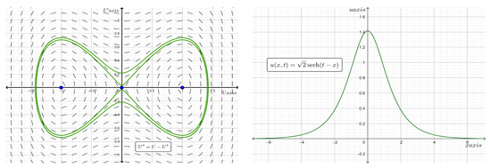
Figure 1. Phase plane diagram (on the left) of the traveling wave system for Equation (10) and the two-dimensional plot (on the right) of the analytic bell type solitary wave solution for the case where $D=1,\kappa =1,\beta =1,$ and $B=\sqrt{2}$ at time $t=0$.

Moreover, the reaction–diffusion–advection equation given by

$$\frac{\partial }{\partial t}u(x,t)-\mathit{D}\frac{{\partial }^2}{\partial x^2}u(x,t)+\beta \frac{\partial }{\partial x}u(x,t)=2\mathit{D}{\kappa }^{2}u(x,t)-\frac{3\sqrt{2}\eta {\kappa }^2\mathit{D}{u}^2(x,t)}{B}+\frac{2\mathit{D}{\kappa }^2{u}^3(x,t)}{B^2},$$

(12)

also has an analytic solution

$$\begin{array}{c}\hfill u(x,t)=\frac{\eta B}{\sqrt{2}}+Bsech\left(\beta \kappa t-\kappa x\right),\end{array}$$

which is a localized solitary wave of the bell type, traveling at any velocity $\beta \ne 0$, where $\eta =\pm 1$. Clearly, ${u(x,t)|}_{t=0}$ approaches $\frac{\eta B}{\sqrt{2}}$ as $x\to \pm \infty$. The proliferation rate $f\left(u\right)$ is a cubic function with three roots, namely, $0,\sqrt{2}B,$ and $\frac{1}{\sqrt{2}}B$. Figure 2 shows the phase portraits of the traveling wave systems for Equation (12) and the two-dimensional plots of the analytic bell type solitary wave solutions when $D=\kappa =\beta =\eta =1,$ and $B=\frac{1}{\sqrt{2}}$ or $B=\sqrt{2}$ at time $t=0$. Additionally, when $\beta =0,$ we find $\omega =0$, and thus, a standing wave solution exists for the reaction–diffusion equation given by

$$\frac{\partial }{\partial t}u(x,t)-\mathit{D}\frac{{\partial }^2}{\partial x^2}u(x,t)=2\mathit{D}{\kappa }^{2}u(x,t)-\frac{3\sqrt{2}\eta {\kappa }^2\mathit{D}{u}^2(x,t)}{B}+\frac{2\mathit{D}{\kappa }^2{u}^3(x,t)}{B^2}.$$

(13)

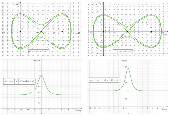
Figure 2. Phase plane diagrams (top plots) of the traveling wave systems for Equation (12) and two-dimensional plots (bottom plots) of the analytic bell type solitary wave solutions at time $t=0$. The left plots show the case where $D=1,\kappa =1,\beta =1,\eta =1,$ and $B=\frac{1}{\sqrt{2}}$, and the right plots show the case where $D=1,\kappa =1,\beta =1,\eta =1,$ and $B=\sqrt{2}$.

Another solitary wave solution of the bell type can be obtained by substituting the trial function of the form

$$U\left(\xi \right)=E-\frac{A{\xi }^2}{B+C{\xi }^2},$$

in Equation (9), assuming $\omega =-\beta \kappa .$ We obtain the following equation

$$\begin{array}{cc}\hfill & (-C^3{E}^3\alpha {}_3+3A{C}^2{E}^2\alpha {}_3-C^3{E}^2\alpha {}_2-3A^{2}CE\alpha {}_3+2A{C}^{2}E\alpha {}_2-C^{3}E\alpha {}_1+A^3\alpha {}_3-A^{2}C\alpha {}_2\hfill \\ & +A{C}^2\alpha {}_1){\xi }^6+(-3B{C}^2{E}^3\alpha {}_3+6ABC{E}^2\alpha {}_3-3B{C}^2{E}^2\alpha {}_2-3A^{2}BE\alpha {}_3+4ABCE\alpha {}_2\hfill \\ & -3B{C}^{2}E\alpha {}_1-A^{2}B\alpha {}_2+2ABC\alpha {}_1){\xi }^4+(-3B^{2}C{E}^3\alpha {}_3+3A{B}^2{E}^2\alpha {}_3-6ABCD{\kappa }^2-3B^{2}C{E}^2\alpha {}_2\hfill \\ & +2A{B}^{2}E\alpha {}_2-3B^{2}CE\alpha {}_1+A{B}^2\alpha {}_1){\xi }^2-B^3{E}^3\alpha {}_3+2A{B}^{2}D{\kappa }^2-B^3{E}^2\alpha {}_2-B^{3}E\alpha {}_1=0.\hfill \end{array}$$

Hence, we obtain the following system of algebraic equations for $\kappa ,{\alpha }_1,{\alpha }_2,{\alpha }_3,A,B,C,D,$ and E:

$$\begin{array}{cc}\hfill & (-C^3{E}^3+3A{C}^2{E}^2-3A^{2}CE+A^3)\alpha {}_3+(-C^3{E}^2+2A{C}^{2}E-A^{2}C)\alpha {}_2+(-C^{3}E+A{C}^2)\alpha {}_1=0,\hfill \\ & (-3B{C}^2{E}^3+6ABC{E}^2-3A^{2}BE)\alpha {}_3+(-3B{C}^2{E}^2+4ABCE-A^{2}B)\alpha {}_2+(-3B{C}^{2}E+2ABC)\alpha {}_1=0,\hfill \\ & (-3B^{2}C{E}^3+3A{B}^2{E}^2)\alpha {}_3+(-3B^{2}C{E}^2+2A{B}^{2}E)\alpha {}_2+(-3B^{2}CE+A{B}^2)\alpha {}_1-6ABCD{\kappa }^2=0,\hfill \\ & -B^3{E}^3\alpha {}_3-B^3{E}^2\alpha {}_2-B^{3}E\alpha {}_1+2A{B}^{2}D{\kappa }^2=0.\hfill \end{array}$$

Solving the resulting system with the aid of Maple, we obtain two solutions, which are described separately below:

$$A=CE,\alpha {}_1=0,\alpha {}_2=-\frac{6CD{\kappa }^2}{BE},\alpha {}_3=\frac{8CD{\kappa }^2}{B{E}^2}$$

and

$$E=\frac{A}{4C},\alpha {}_1=\frac{9CD{\kappa }^2}{2B},\alpha {}_2=\frac{12C^{2}D{\kappa }^2}{AB},\alpha {}_3=\frac{8C^{3}D{\kappa }^2}{A^{2}B},$$

where $\omega =-\beta \kappa$ and $A,B,C,D,E,\kappa ,$ and $\beta$ are arbitrary nonzero real numbers.

Therefore, the reaction–diffusion–advection equation given by

$$\begin{array}{cc}\hfill \frac{\partial }{\partial t}u(x,t)-\mathit{D}\frac{{\partial }^2}{\partial x^2}u(x,t)+\beta \frac{\partial }{\partial x}u(x,t)& =\frac{-6CD{\kappa }^2{u}^2(x,t)}{BE}+\frac{8CD{\kappa }^2{u}^3(x,t)}{B{E}^2},\hfill \end{array}$$

(14)

has the analytic solution

$$\begin{array}{c}\hfill u(x,t)=E-\frac{CE{\left(\kappa x-\beta \kappa t\right)}^2}{B+C{\left(\kappa x-\beta \kappa t\right)}^2},\end{array}$$

which is a localized solitary wave of the bell type, traveling at any velocity $\beta \ne 0$. The proliferation rate $f\left(u\right)$ is a cubic function with roots of 0 (with multiplicity of 2) and $\frac{3}{4}E$. In particular, when $E=\frac{4}{3}$, $f\left(u\right)$ has the roots 0 and 1, and hence, $f\left(u\right)$ is a cubic function with a reverse weak Allee effect. Figure 3 shows the phase portrait of the traveling wave system for Equation (14) and the two-dimensional plot of the analytic bell type solitary wave solution along with the graph of the proliferation rate $f\left(u\right)$ for the case where $D=B=C=\kappa =\beta =1,$ and $E=\frac{4}{3}$ at time $t=0$. Additionally, when $\beta =0,$ we find $\omega =0$, and thus, a standing wave solution exists for the reaction–diffusion equation given by

$$\frac{\partial }{\partial t}u(x,t)-\mathit{D}\frac{{\partial }^2}{\partial x^2}u(x,t)=\frac{-6CD{\kappa }^2{u}^2(x,t)}{BE}+\frac{8CD{\kappa }^2{u}^3(x,t)}{B{E}^2}.$$

(15)

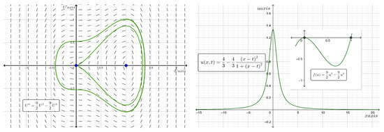
Figure 3. Phase plane diagram (on the left) of the traveling wave system for Equation (14) and the two-dimensional plot (on the right) of the analytic bell type solitary wave solution along with the graph of $f\left(u\right)$ for the case where $D=B=C=\kappa =\beta =1,$ and $E=\frac{4}{3}$ at time $t=0$.

Moreover, the reaction–diffusion–advection equation given by

$$\begin{array}{cc}\hfill \frac{\partial }{\partial t}u(x,t)-\mathit{D}\frac{{\partial }^2}{\partial x^2}u(x,t)& +\beta \frac{\partial }{\partial x}u(x,t)=\frac{9CD{\kappa }^{2}u\left(x,t\right)}{2B}\hfill \\ & +\frac{12C^{2}D{\kappa }^2{u}^2(x,t)}{AB}+\frac{8C^{3}D{\kappa }^2{u}^3(x,t)}{A^{2}B},\hfill \end{array}$$

(16)

has the analytic solution

$$\begin{array}{c}\hfill u(x,t)=\frac{A}{4C}-\frac{A{\left(\kappa x-\beta \kappa t\right)}^2}{B+C{\left(\kappa x-\beta \kappa t\right)}^2},\end{array}$$

which is a localized solitary wave of the bell type, traveling at any velocity $\beta \ne 0$. The proliferation rate $f\left(u\right)$ is a cubic function with roots of 0 and $-\frac{3A}{4C}$ (with multiplicity of 2). In particular, when $A=-\frac{4}{3}C>0$, $f\left(u\right)$ has the roots 0 and 1, and hence, $f\left(u\right)$ is a cubic function with a weak Allee effect. Figure 4 shows the phase portrait of the traveling wave system for Equation (16) and the two-dimensional plot of the analytic bell type solitary wave solution along with the graph of the proliferation rate $f\left(u\right)$ for the case where $D=B=C=E=\kappa =\beta =1,$ and $A=-\frac{4}{3}$ at time $t=0$. Additionally, when $\beta =0,$ we find $\omega =0$, and thus, a standing wave solution exists for the reaction–diffusion equation given by

$$\frac{\partial }{\partial t}u(x,t)-\mathit{D}\frac{{\partial }^2}{\partial x^2}u(x,t)=\frac{9CD{\kappa }^{2}u\left(x,t\right)}{2B}+\frac{12C^{2}D{\kappa }^2{u}^2(x,t)}{AB}+\frac{8C^{3}D{\kappa }^2{u}^3(x,t)}{A^{2}B}.$$

(17)

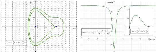
Figure 4. Phase plane diagram (on the left) of the traveling wave system for Equation (16) and the two-dimensional plot (on the right) of the analytic bell type solitary wave solution along with the graph of $f\left(u\right)$ for the case where $D=B=C=E=\kappa =\beta =1,$ and $A=-\frac{4}{3}$ at time $t=0$.

On the other hand, in order to obtain solitary waves of the kink type, we substitute the trial function of the form

$$U\left(\xi \right)=A+Btanh\left(\xi \right),$$

in (9) and obtain the following equation

$$\begin{array}{cc}\hfill & \left(-B^3{\alpha }_3-2B\mathit{D}{\kappa }^2\right){tanh}^3\left(\xi \right)+\left(-\left(\beta \kappa +\omega \right)B-{\alpha }_2{B}^2-3{\alpha }_{3}A{B}^2\right){tanh}^2\left(\xi \right)\hfill \\ & +\left(-3A^{2}B{\alpha }_3+2B\mathit{D}{\kappa }^2-2AB{\alpha }_2-B{\alpha }_1\right)tanh\left(\xi \right)+\left(\beta \kappa +\omega \right)B-{\alpha }_{1}A-{\alpha }_2{A}^2-{\alpha }_3{A}^3=0.\hfill \end{array}$$

Hence, we obtain the following system of algebraic equations for $\beta ,\kappa ,\omega ,{\alpha }_1,{\alpha }_2,{\alpha }_3,D,A,$ and B:

$$\begin{array}{cc}\hfill & -B^3{\alpha }_3-2B\mathit{D}{\kappa }^2=0,\hfill \\ & -\left(\beta \kappa +\omega \right)B-{\alpha }_2{B}^2-3{\alpha }_{3}A{B}^2=0,\hfill \\ & -3A^{2}B{\alpha }_3+2B\mathit{D}{\kappa }^2-2AB{\alpha }_2-B{\alpha }_1=0,\hfill \\ & \left(\beta \kappa +\omega \right)B-{\alpha }_{1}A-{\alpha }_2{A}^2-{\alpha }_3{A}^3=0.\hfill \end{array}$$

Solving the resulting system with the aid of Maple, we obtain two solutions, which are described separately below:

$$\omega =\frac{\kappa \left(2A\mathit{D}\kappa -B\beta \right)}{B},{\alpha }_1=\frac{-2\mathit{D}{\kappa }^2\left(A^2-B^2\right)}{B^2},{\alpha }_2=\frac{4\mathit{D}{\kappa }^{2}A}{B^2},{\alpha }_3=\frac{-2\mathit{D}{\kappa }^2}{B^2}$$

and

$$A=\eta B,{\alpha }_1=-4\mathit{D}{\kappa }^2+\eta \left(2\beta \kappa +2\omega \right),{\alpha }_2=\frac{6\mathit{D}\eta {\kappa }^2-\beta \kappa -\omega }{B},{\alpha }_3=\frac{-2\mathit{D}{\kappa }^2}{B^2},$$

where $\beta ,\kappa ,\omega ,D,A,$ and B are arbitrary nonzero constants and $\eta =\pm 1$.

Therefore, the reaction–diffusion–advection equation given by

$$\begin{array}{cc}\hfill \frac{\partial }{\partial t}u(x,t)-\mathit{D}\frac{{\partial }^2}{\partial x^2}u(x,t)+\beta \frac{\partial }{\partial x}u(x,t)& =\frac{-2\mathit{D}{\kappa }^2\left(A^2-B^2\right)u(x,t)}{B^2}\hfill \\ & +\frac{4\mathit{D}{\kappa }^{2}A{u}^2(x,t)}{B^2}-\frac{2\mathit{D}{\kappa }^2{u}^3(x,t)}{B^2},\hfill \end{array}$$

(18)

has the analytic solution

$$\begin{array}{c}\hfill u(x,t)=A+Btanh\left(\kappa x+\frac{\kappa \left(2A\mathit{D}\kappa -B\beta \right)}{B}t\right),\end{array}$$

which is a localized solitary wave of the kink (anti-kink) type. Here, the proliferation rate $f\left(u\right)$ has three roots, namely, 0 and $A\pm B$. In particular, when $A=\frac{\lambda +1}{2\lambda }$ and $B=\frac{\eta (\lambda -1)}{2\lambda }$, where $\lambda$ is a number greater than 1 and $\eta =\pm 1$, $f\left(u\right)$ has the roots $0,{\lambda }^{-1},$ and 1, and hence, $f\left(u\right)$ is a cubic function with a strong Allee effect. Consequently, the kink (anti-kink) solution is a solitary wave with asymptotic values ${\lambda }^{-1}$ and 1 at the left and right infinities. Additionally, when $\lambda =\frac{\beta \eta +2\mathit{D}\kappa }{\beta \eta -2\mathit{D}\kappa },$ we find $\omega =0$ and thus, a standing wave solution exists. In addition, from Equation (18), when $\beta =0$, a solitary wave of the kink (anti-kink) type can be obtained for the reaction–diffusion equation

$$\begin{array}{cc}\hfill \frac{\partial }{\partial t}u(x,t)-\mathit{D}\frac{{\partial }^2}{\partial x^2}u(x,t)& =\frac{-2\mathit{D}{\kappa }^2\left(A^2-B^2\right)u(x,t)}{B^2}\hfill \\ & +\frac{4\mathit{D}{\kappa }^{2}A{u}^2(x,t)}{B^2}-\frac{2\mathit{D}{\kappa }^2{u}^3(x,t)}{B^2},\hfill \end{array}$$

(19)

and, hence, when $\omega =0$, a standing wave solution exists. Figure 5 shows the phase portraits of the traveling wave system for Equation (18) and the two-dimensional plot of the analytic kink type solitary wave solutions along with the graph of the proliferation rate $f\left(u\right)$ for the case where $D=\kappa =\beta =\eta =1,$ and $\lambda =4$ at time $t=0$.

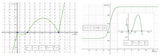
Figure 5. Phase plane diagram (on the left) of the traveling wave system for Equation (18) and the two-dimensional plot (on the right) of the analytic kink type solitary wave solution along with the graph of $f\left(u\right)$ for the case where $D=\kappa =\beta =\eta =1,$ and $\lambda =4$ at time $t=0$.

Moreover, the reaction–diffusion–advection equation given by

$$\begin{array}{cc}\hfill \frac{\partial }{\partial t}u(x,t)-\mathit{D}\frac{{\partial }^2}{\partial x^2}u(x,t)+\beta \frac{\partial }{\partial x}u(x,t)& =(-4\mathit{D}{\kappa }^2+\eta \left(2\beta \kappa +2\omega \right))u(x,t)\hfill \\ & +\frac{\left(6\mathit{D}\eta {\kappa }^2-\beta \kappa -\omega \right)u^2(x,t)}{B}-\frac{2\mathit{D}{\kappa }^2{u}^3(x,t)}{B^2},\hfill \end{array}$$

(20)

has the analytic solution

$$\begin{array}{c}\hfill u(x,t)=\eta B+Btanh\left(\kappa x+\omega t\right),\end{array}$$

which is a localized solitary wave of the kink (anti-kink) type. Here, the proliferation rate $f\left(u\right)$ has three roots, namely, $0,2\eta B,$ and $\frac{B}{2\mathit{D}{\kappa }^2}\left(2\eta \mathit{D}{\kappa }^2-\beta \kappa -\omega \right)$, where $\eta =\pm 1$. Thus, there are three cases, as shown below:

• When $\omega =\kappa \left(2\mathit{D}\eta \kappa -\beta \right)$ and $B=\frac{\eta }{2}$, then $f\left(u\right)$ has the roots 0 (with a multiplicity of 2) and 1, and hence, $f\left(u\right)$ is a cubic function with a weak Allee effect. Consequently, the kink (anti-kink) solution is a solitary wave with asymptotic values of 0 and 1 at the left and right infinities. On the other hand, when $\beta =2\mathit{D}\eta \kappa$, we find $\omega =0$, and thus, a standing wave solution exists. Moreover, when $\omega =\kappa \left(-2\mathit{D}\eta \kappa -\beta \right)$ and $B=\frac{\eta }{2}$, $f\left(u\right)$ has the roots 1 (with a multiplicity of 2) and 0, and hence, $f\left(u\right)$ is a cubic function with a reverse weak Allee effect. Consequently, the kink (anti-kink) solution is a solitary wave with asymptotic values of 0 and 1 at the left and right infinities. Hence, a standing wave solution can be obtained for the case where $\beta =-2\mathit{D}\eta \kappa$. Figure 6 shows the phase portraits of the traveling wave system for Equation (20) and the two-dimensional plot of the analytic kink type solitary wave solutions along with the graph of the proliferation rate $f\left(u\right)$ for the case where $D=\kappa =\beta =\eta =1$ at time $t=0$.
  

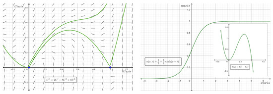  Figure 6. Phase plane diagram (on the left) of the traveling wave system for Equation (20) and the two-dimensional plot (on the right) of the analytic kink type solitary wave solution along with the graph of $f\left(u\right)$ for the case where $D=\kappa =\beta =\eta =1$ at time $t=0$.
• When $\omega =\frac{\kappa }{\lambda }\left(2\mathit{D}\lambda \eta \kappa -4\mathit{D}\eta \kappa -\lambda \beta \right)$ and $B=\frac{\eta }{2}$, where a number $\lambda >1$, $f\left(u\right)$ has the roots $0,{\lambda }^{-1},$ and 1, and hence, $f\left(u\right)$ is a cubic function with a strong Allee effect. Consequently, the kink (anti-kink) solution is a solitary wave with asymptotic values of 0 and 1 at the left and right infinities. On the other hand, when $\beta =\frac{1}{\lambda }\left(2\mathit{D}\lambda \eta \kappa -4\mathit{D}\eta \kappa \right)$, we find $\omega =0$, and thus, a standing wave solution exists. Figure 7 shows the phase portraits of the traveling wave system for Equation (20) and the two-dimensional plot of the analytic kink type solitary wave solutions along with the graph of the proliferation rate $f\left(u\right)$ for the case where $D=2,\kappa =\beta =\eta =1,$ and $\lambda =4$ at time $t=0$.
  

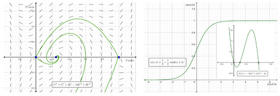  Figure 7. Phase plane diagram (on the left) of the traveling wave system for Equation (20) and the two-dimensional plot (on the right) of the analytic kink type solitary wave solution along with the graph of $f\left(u\right)$ for the case where $D=2,\kappa =\beta =\eta =1,$ and $\lambda =4$ at time $t=0$.
• When $\omega =\kappa \left(-4\mathit{D}\lambda \eta \kappa +2\mathit{D}\eta \kappa -\beta \right)$ and $B=\frac{\eta }{2\lambda }$, where $\lambda$ is a number greater than 1, $f\left(u\right)$ has the roots $0,{\lambda }^{-1},$ and 1, and hence, $f\left(u\right)$ is a cubic function with a strong Allee effect. Consequently, the kink (anti-kink) solution is a solitary wave with asymptotic values of 0 and ${\lambda }^{-1}$ at the left and right infinities. On the other hand, when $\beta =-4\mathit{D}\lambda \eta \kappa +2\mathit{D}\eta \kappa$, we find $\omega =0$, and thus, a standing wave solution exists. Figure 8 shows the phase portraits of the traveling wave system for Equation (20) and the two-dimensional plot of the analytic kink type solitary wave solutions along with the graph of the proliferation rate $f\left(u\right)$ for the case where $D=1,\kappa =\beta =\eta =1,$ and $\lambda =4$ at time $t=0$.
  

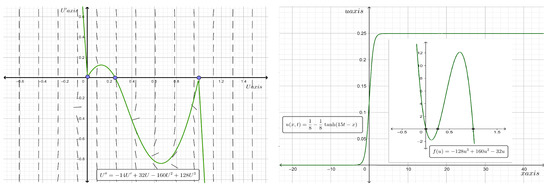  Figure 8. Phase plane diagram (on the left) of the traveling wave system for Equation (20) and the two-dimensional plot (on the right) of the analytic kink type solitary wave solution along with the graph of $f\left(u\right)$ for the case where $D=\kappa =\beta =\eta =1,$ and $\lambda =4$ at time $t=0$.

On the other hand, as shown in Equation (20), when $\beta =0$, solitary waves of the kink (anti-kink) type can be obtained for the reaction–diffusion equation

$$\begin{array}{cc}\hfill \frac{\partial }{\partial t}u(x,t)-\mathit{D}\frac{{\partial }^2}{\partial x^2}u(x,t)& =(-4\mathit{D}{\kappa }^2+\eta \left(2\beta \kappa +2\omega \right))u(x,t)\hfill \\ & +\frac{\left(6\mathit{D}\eta {\kappa }^2-\beta \kappa -\omega \right)u^2(x,t)}{B}-\frac{2\mathit{D}{\kappa }^2{u}^3(x,t)}{B^2}.\hfill \end{array}$$

(21)

Here, there are three cases, as previously explained, and the difference is only in the value of $\beta$. For the sake of brevity, we omit the details.

Form II. 

Here, we consider the reaction–diffusion–advection model of the form

$$\frac{\partial }{\partial t}u(x,t)-\mathit{D}\frac{{\partial }^2}{\partial x^2}u(x,t)+\beta \frac{\partial }{\partial x}u(x,t)={\alpha }_{1}u(x,t)+{\alpha }_2{u}^2(x,t),$$

(22)

where ${\alpha }_1$ and ${\alpha }_2$ are constants to be determined later. As opposed to Form I, Equations (8) and (22) do not have a cubic term in u. As before, by using the transformation $u(x,t)=U\left(\xi \right)$, where $\xi =\kappa x+\omega t$, Equation (22) is converted to the equation

$$\left(\beta \kappa +\omega \right)\frac{\mathrm{d}}{\mathrm{d}\xi }U\left(\xi \right)-D{\kappa }^2\frac{{\mathrm{d}}^2}{\mathrm{d}{\xi }^2}U\left(\xi \right)={\alpha }_{1}U\left(\xi \right)+{\alpha }_2{U}^2\left(\xi \right).$$

(23)

Substituting the trial function given by

$$U\left(\xi \right)=A+Bsec{h}^2\left(\xi \right),$$

into Equation (23), we obtain

$$\begin{array}{cc}\hfill & \left(6B\mathit{D}{\kappa }^2-B^2{\alpha }_2\right){\mathrm{sech}}^4\left(\xi \right)+\left(-2\left(\beta \kappa +\omega \right)Btanh\left(\xi \right)-2{\alpha }_{2}AB-{\alpha }_{1}B-4B\mathit{D}{\kappa }^2\right){\mathrm{sech}}^2\left(\xi \right)\hfill \\ & -{\alpha }_2{A}^2-{\alpha }_{1}A=0.\hfill \end{array}$$

As a result, we obtain the following system of algebraic equations for $\beta$, $\kappa ,\omega$, ${\alpha }_1,{\alpha }_2,D,A,$ and B:

$$\begin{array}{cc}\hfill & 6B\mathit{D}{\kappa }^2-B^2{\alpha }_2=0,\hfill \\ & -2\left(\beta \kappa +\omega \right)B=0,\hfill \\ & -2{\alpha }_{2}AB-{\alpha }_{1}B-4B\mathit{D}{\kappa }^2=0,\hfill \\ & -{\alpha }_2{A}^2-{\alpha }_{1}A=0.\hfill \end{array}$$

Solving the resulting system with the aid of Maple, we obtain two solutions, which are described separately below:

$$\omega =-\beta \kappa ,A=0,{\alpha }_1=-4\mathit{D}{\kappa }^2,{\alpha }_2=\frac{6\mathit{D}{\kappa }^2}{B}$$

and

$$\omega =-\beta \kappa ,A=\frac{-2B}{3},{\alpha }_1=4\mathit{D}{\kappa }^2,{\alpha }_2=\frac{6\mathit{D}{\kappa }^2}{B},$$

where $\beta ,\kappa ,D,$ and B are arbitrary nonzero constants.

Therefore, the reaction–diffusion–advection equation given by

$$\frac{\partial }{\partial t}u(x,t)-\mathit{D}\frac{{\partial }^2}{\partial x^2}u(x,t)+\beta \frac{\partial }{\partial x}u(x,t)=-4\mathit{D}{\kappa }^{2}u(x,t)+\frac{6\mathit{D}{\kappa }^2{u}^2(x,t)}{B},$$

(24)

has the analytic solution

$$\begin{array}{c}\hfill u(x,t)=Bsec{h}^2\left(\beta \kappa t-\kappa x\right),\end{array}$$

which is a localized solitary wave of the bell type, traveling at any velocity $\beta \ne 0$. Clearly, ${u(x,t)|}_{t=0}$, along with its derivative, approaches zero as $x\to \pm \infty$. The proliferation rate $f\left(u\right)$ is a quadratic function with reverse logistic growth that has two roots, namely, 0 and $\frac{2B}{3}$. Figure 9 shows the phase portraits of the traveling wave system for Equation (24) and the two-dimensional plot of the analytic bell type solitary wave solution for the case where $D=\kappa =\beta =1,$ and $B=\frac{3}{2}$ at time $t=0$. Additionally, when $\beta =0,$ we find $\omega =0$, and thus, a standing wave solution exists for the reaction–diffusion equation given by

$$\frac{\partial }{\partial t}u(x,t)-\mathit{D}\frac{{\partial }^2}{\partial x^2}u(x,t)=-4\mathit{D}{\kappa }^{2}u(x,t)+\frac{6\mathit{D}{\kappa }^2{u}^2(x,t)}{B},$$

(25)

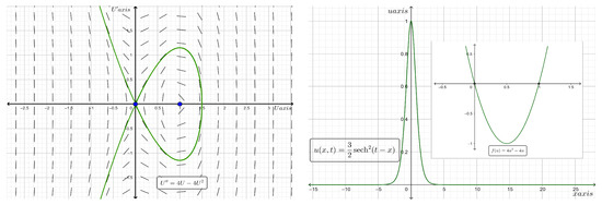
Figure 9. Phase plane diagram (on the left) of the traveling wave system for Equation (24) and the two-dimensional plot (on the right) of the analytic bell type solitary wave solution for the case where $D=1,\kappa =1,\beta =1,$ and $B=\frac{3}{2}$ at time $t=0$.

Moreover, the reaction–diffusion–advection equation given by

$$\frac{\partial }{\partial t}u(x,t)-\mathit{D}\frac{{\partial }^2}{\partial x^2}u(x,t)+\beta \frac{\partial }{\partial x}u(x,t)=4\mathit{D}{\kappa }^{2}u(x,t)+\frac{6\mathit{D}{\kappa }^2{u}^2(x,t)}{B},$$

(26)

has the analytic solution

$$\begin{array}{c}\hfill u(x,t)=\frac{-2B}{3}+Bsec{h}^2\left(\beta \kappa t-\kappa x\right),\end{array}$$

which is a localized solitary wave of the bell type, traveling at any velocity $\beta \ne 0$. It is obvious that ${u(x,t)|}_{t=0}$ approaches $\frac{-2B}{3}$ as $x\to \pm \infty$. The proliferation rate $f\left(u\right)$ is a quadratic function with logistic growth that has two roots, namely, 0 and $-\frac{2B}{3}$. Figure 10 shows the phase portraits of the traveling wave system for Equation (26) and the two-dimensional plot of the analytic bell type solitary wave solution for the case where $D=\kappa =\beta =1,$ and $B=-\frac{3}{2}$ at time $t=0$. Additionally, when $\beta =0,$ we find $\omega =0$ and thus, a standing wave solution exists for the reaction–diffusion equation given by

$$\frac{\partial }{\partial t}u(x,t)-\mathit{D}\frac{{\partial }^2}{\partial x^2}u(x,t)=4\mathit{D}{\kappa }^{2}u(x,t)+\frac{6\mathit{D}{\kappa }^2{u}^2(x,t)}{B}.$$

(27)

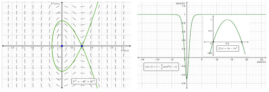
Figure 10. Phase plane diagram (on the left) of the traveling wave system for Equation (26) and the two-dimensional plot (on the right) of the analytic bell type solitary wave solution for the case where $D=1,\kappa =1,\beta =1,$ and $B=-\frac{3}{2}$ at time $t=0$.

Form III. 

Now, let us consider the reaction–diffusion–advection model of the form

$$\frac{\partial }{\partial t}u(x,t)-\mathit{D}\frac{{\partial }^2}{\partial x^2}u(x,t)+\beta \frac{\partial }{\partial x}u(x,t)=(u(x,t)-{\alpha }_1)(u(x,t)-{\alpha }_2)(1-u(x,t)),$$

(28)

where ${\alpha }_1$ and ${\alpha }_2$ are constants to be determined later. By using the transformation $u(x,t)=U\left(\xi \right),$ where $\xi =\kappa x+\omega t,$ we change Equation (28) into the ordinary differential equation

$$\left(\beta \kappa +\omega \right)\frac{\mathrm{d}}{\mathrm{d}\xi }U\left(\xi \right)-D{\kappa }^2\frac{{\mathrm{d}}^2}{\mathrm{d}{\xi }^2}U\left(\xi \right)=(U\left(\xi \right)-{\alpha }_1)(U\left(\xi \right)-{\alpha }_2)(1-U\left(\xi \right)).$$

(29)

Then, we substitute the trial function given by

$$U\left(\xi \right)=A+Btanh\left(\xi \right),$$

into Equation (29) and obtain the following equation

$$\begin{array}{cc}\hfill & \left(-2BD{\kappa }^2+B^3\right){tanh}^3\left(\xi \right)+\left(-\left(\beta \kappa +\omega \right)B+\left(\left(A-\alpha {}_1\right)B+B\left(A-\alpha {}_2\right)\right)B-B^2\left(-A+1\right)\right){tanh}^2\left(\xi \right)\hfill \\ & +\left(2BD{\kappa }^2+\left(A-\alpha {}_1\right)\left(A-\alpha {}_2\right)B-\left(\left(A-\alpha {}_1\right)B+B\left(A-\alpha {}_2\right)\right)\left(-A+1\right)\right)tanh\left(\xi \right)\hfill \\ & +\left(\beta \kappa +\omega \right)B-\left(A-\alpha {}_1\right)\left(A-\alpha {}_2\right)\left(-A+1\right)=0,\hfill \end{array}$$

where A and B are constants to be determined later. Hence, we obtain the following system of algebraic equations for $\beta ,\kappa ,\omega ,{\alpha }_1,{\alpha }_2,A,B,$ and D:

$$\begin{array}{cc}\hfill & B^3-2BD{\kappa }^2=0,\hfill \\ & 3AB-B\alpha {}_1-B\alpha {}_2-\beta \kappa -B-\omega =0,\hfill \\ & 2BD{\kappa }^2+\left(A-\alpha {}_1\right)\left(A-\alpha {}_2\right)B-\left(\left(A-\alpha {}_1\right)B+B\left(A-\alpha {}_2\right)\right)\left(-A+1\right)=0,\hfill \\ & \left(\beta \kappa +\omega \right)B-\left(A-\alpha {}_1\right)\left(A-\alpha {}_2\right)\left(-A+1\right)=0.\hfill \end{array}$$

Solving this system, we obtain two solutions:

$$A=Bϵ+1,D=\frac{B^2}{2{\kappa }^2},\alpha {}_1=2Bϵ+1,\omega =B^2ϵ-B\alpha {}_2-\beta \kappa +B$$

and

$$A=Bϵ+\alpha {}_2,D=\frac{B^2}{2{\kappa }^2},\alpha {}_1=2Bϵ+\alpha {}_2,\omega =B^2ϵ+B\alpha {}_2-\beta \kappa -B,$$

where $ϵ=\pm 1$ and $\beta ,\kappa ,B,$ and ${\alpha }_2$ are arbitrary nonzero constants.

Therefore, the reaction–diffusion–advection equation given by

$$\begin{array}{cc}\hfill & \frac{\partial }{\partial t}u(x,t)-\frac{B^2}{2{\kappa }^2}\frac{{\partial }^2}{\partial x^2}u(x,t)+\beta \frac{\partial }{\partial x}u(x,t)=\left(u(x,t)-2Bϵ-1\right)\left(u(x,t)-\alpha {}_2\right)\left(1-u(x,t)\right),\hfill \end{array}$$

(30)

has the analytic solution

$$\begin{array}{c}\hfill u(x,t)=1+Bϵ+Btanh\left(\kappa x+\left(B^2ϵ-B\alpha {}_2-\beta \kappa +B\right)t\right),\end{array}$$

which is a localized solitary wave of the kink (anti-kink) type. In particular, when $B=\frac{ϵ\left(1-\lambda \right)}{2\lambda },\kappa =\frac{\eta \sqrt{2}B}{2},{\alpha }_2={\mu }^{-1}$, where $\lambda >\mu >1$ and $\eta =\pm 1$. $f\left(u\right)$ has the roots ${\lambda }^{-1},{\mu }^{-1},$ and 1 and hence, $f\left(u\right)$ is a cubic function with a higher-order Allee effect. Consequently, the solution constructed when $\eta =1$ is a solitary wave of the kink type that is moving at a constant wave speed is determined by the formula $v=-\frac{\omega }{\kappa }=\frac{\sqrt{2}}{2}\left(\beta \sqrt{2}-1\right)+\frac{\sqrt{2}}{\mu }-\frac{\sqrt{2}}{2\lambda }$ has asymptotic values of ${\lambda }^{-1}$ and 1 at the left and right infinities, whereas the solution constructed when $\eta =-1$ is a solitary wave of the anti-kink type that is moving at a constant wave speed determined by the formula $v=-\frac{\omega }{\kappa }=\frac{\sqrt{2}}{2}\left(\beta \sqrt{2}+1\right)-\frac{\sqrt{2}}{\mu }+\frac{\sqrt{2}}{2\lambda }$ has asymptotic values of 1 and ${\lambda }^{-1}$ at the left and right infinities. On the other hand, when $\beta =\frac{B}{\kappa }\left(Bϵ-\alpha {}_2+1\right)$, we find $\omega =0$, and thus, a standing wave solution exists. Figure 11 shows the phase portraits of the traveling wave system for Equation (30) and the two-dimensional plot of the analytic kink type solitary wave solutions along with the graph of the proliferation rate $f\left(u\right)$ for the case where $\beta =\eta =ϵ=1,\mu =2,$ and $\lambda =4$ at time $t=0$. Additionally, from Equation (30), when $\beta =0$, a solitary wave of the kink (anti-kink) type can be obtained for the reaction–diffusion equation

$$\begin{array}{cc}\hfill & \frac{\partial }{\partial t}u(x,t)-\frac{B^2}{2{\kappa }^2}\frac{{\partial }^2}{\partial x^2}u(x,t)=\left(u(x,t)-2Bϵ-1\right)\left(u(x,t)-\alpha {}_2\right)\left(1-u(x,t)\right).\hfill \end{array}$$

(31)

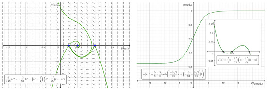
Figure 11. Phase plane diagram (on the left) of the traveling wave system for Equation (30) and the two-dimensional plot (on the right) of the analytic kink type solitary wave solution along with the graph of $f\left(u\right)$ for the case where $\beta =\eta =ϵ=1,\mu =2,$ and $\lambda =4$ at time $t=0$.

Moreover, the reaction–diffusion–advection equation given by

$$\begin{array}{cc}\hfill & \frac{\partial }{\partial t}u(x,t)-\frac{B^2}{2{\kappa }^2}\frac{{\partial }^2}{\partial x^2}u(x,t)+\beta \frac{\partial }{\partial x}u(x,t)=\left(u(x,t)-2Bϵ-\alpha {}_2\right)\left(u(x,t)-\alpha {}_2\right)\left(1-u(x,t)\right),\hfill \end{array}$$

(32)

has the analytic solution

$$\begin{array}{c}\hfill u(x,t)=\alpha {}_2+Bϵ+Btanh\left(\kappa x+\left(B^2ϵ+B\alpha {}_2-\beta \kappa -B\right)t\right),\end{array}$$

which is a localized solitary wave of the kink (anti-kink) type. In particular, when $B=\frac{ϵ\left(\mu -\lambda \right)}{2\lambda \mu },\kappa =\frac{\eta \sqrt{2}B}{2},{\alpha }_2={\mu }^{-1}$, where $\lambda >\mu >1$ and $\eta =\pm 1$. $f\left(u\right)$ has the roots ${\lambda }^{-1},{\mu }^{-1},$ and 1, and hence, $f\left(u\right)$ is a cubic function with a higher-order Allee effect. Consequently, the solution constructed when $\eta =1$ is a solitary wave of the kink type that is moving at a constant wave speed determined by the formula $v=-\frac{\omega }{\kappa }=\frac{\sqrt{2}}{2}\left(\beta \sqrt{2}+2\right)-\frac{\sqrt{2}}{2\mu }-\frac{\sqrt{2}}{2\lambda }$ has asymptotic values of ${\lambda }^{-1}$ and ${\mu }^{-1}$ at the left and right infinities, whereas the solution constructed when $\eta =-1$ is a solitary wave of the anti-kink type that is moving at a constant wave speed determined by the formula $v=-\frac{\omega }{\kappa }=\frac{\sqrt{2}}{2}\left(\beta \sqrt{2}-2\right)+\frac{\sqrt{2}}{2\mu }+\frac{\sqrt{2}}{2\lambda }$ has asymptotic values ${\mu }^{-1}$ and ${\lambda }^{-1}$ at the left and right infinities. On the other hand, when $\beta =\frac{B}{\kappa }\left(Bϵ+\alpha {}_2-1\right)$, we find $\omega =0$, and thus, a standing wave solution exists. Figure 12 shows the phase portraits of the traveling wave system for Equation (32) and the two-dimensional plot of the analytic kink type solitary wave solutions along with the graph of the proliferation rate $f\left(u\right)$ for the case where $\beta =\eta =ϵ=1,\mu =2,$ and $\lambda =4$ at time $t=0$. Additionally, from Equation (32), when $\beta =0$, a solitary wave of the kink (anti-kink) type can be obtained for the reaction–diffusion equation

$$\begin{array}{c}\hfill \frac{\partial }{\partial t}u(x,t)-\frac{B^2}{2{\kappa }^2}\frac{{\partial }^2}{\partial x^2}u(x,t)=\left(u(x,t)-2Bϵ-\alpha {}_2\right)\left(u(x,t)-\alpha {}_2\right)\left(1-u(x,t)\right).\end{array}$$

(33)

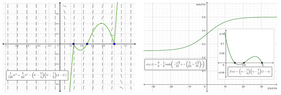
Figure 12. Phase plane diagram (on the left) of the traveling wave system for Equation (32) and the two-dimensional plot (on the right) of the analytic kink type solitary wave solution along with the graph of $f\left(u\right)$ for the case where $\beta =\eta =ϵ=1,\mu =2,$ and $\lambda =4$ at time $t=0$.

Form IV. 

Finally, we consider the reaction–diffusion–advection model of the form

$$\frac{\partial }{\partial t}u(x,t)-\mathit{D}\frac{{\partial }^2}{\partial x^2}u(x,t)+\beta \frac{\partial }{\partial x}u(x,t)={\alpha }_{1}u(x,t)+{\alpha }_3{u}^3(x,t)+{\alpha }_5{u}^5(x,t),$$

(34)

where ${\alpha }_1,{\alpha }_3,$ and ${\alpha }_5$ are constants to be determined later. As before, by using the transformation $u(x,t)=U\left(\xi \right),$ where $\xi =\kappa x+\omega t,$ we change Equation (34) into the ordinary differential equation

$$\left(\beta \kappa +\omega \right)\frac{\mathrm{d}}{\mathrm{d}\xi }U\left(\xi \right)-D{\kappa }^2\frac{{\mathrm{d}}^2}{\mathrm{d}{\xi }^2}U\left(\xi \right)={\alpha }_{1}U\left(\xi \right)+{\alpha }_3{U}^3\left(\xi \right)+{\alpha }_5{U}^5\left(\xi \right).$$

(35)

Then, we use of the trial function given by

$$U\left(\xi \right)=\frac{Aexp\left(\frac{\xi }{4}\right)}{\sqrt{1-Bexp\left(\frac{\xi }{2}\right)}},$$

where A and B are real numbers to be determined later. Substituting the trial function into Equation (35) and simplifying, we obtain the following equation

$$\begin{array}{cc}\hfill & \left(2B\mathit{D}{\kappa }^2+16A^2{\alpha }_3+4B\beta \kappa +4B\omega -32B{\alpha }_1\right)exp\left(\frac{\xi }{2}\right)\hfill \\ & \left(16A^4{\alpha }_5-16A^{2}B{\alpha }_3+16B^2{\alpha }_1\right)exp\left(\xi \right)+\mathit{D}{\kappa }^2-4\beta \kappa -4\omega +16{\alpha }_1=0.\hfill \end{array}$$

Thus, we obtain the following system of algebraic equations for $\beta$, $\kappa ,\omega$, ${\alpha }_1,{\alpha }_3,{\alpha }_5,D,A,$ and B:

$$\begin{array}{cc}\hfill & 16A^4{\alpha }_5-16A^{2}B{\alpha }_3+16B^2{\alpha }_1=0,\hfill \\ & 2B\mathit{D}{\kappa }^2+16A^2{\alpha }_3+4B\beta \kappa +4B\omega -32B{\alpha }_1=0,\hfill \\ & \mathit{D}{\kappa }^2-4\beta \kappa -4\omega +16{\alpha }_1=0.\hfill \end{array}$$

Solving this system, we obtain the following solution:

$${\alpha }_1=\frac{\beta \kappa +\omega }{4}-\frac{\mathit{D}{\kappa }^2}{16},{\alpha }_3=\frac{-B\left(\mathit{D}{\kappa }^2-\beta \kappa -\omega \right)}{4A^2},{\alpha }_5=\frac{-3B^2\mathit{D}{\kappa }^2}{16A^4},$$

where $\beta ,\kappa ,\omega ,D,A,$ and B are arbitrary nonzero constants.

Therefore, the reaction–diffusion–advection equation given by

$$\begin{array}{cc}\hfill & \frac{\partial }{\partial t}u(x,t)-\mathit{D}\frac{{\partial }^2}{\partial x^2}u(x,t)+\beta \frac{\partial }{\partial x}u(x,t)=\hfill \\ & \left(\frac{\beta \kappa +\omega }{4}-\frac{\mathit{D}{\kappa }^2}{16}\right)u(x,t)-\frac{B\left(\mathit{D}{\kappa }^2-\beta \kappa -\omega \right)}{4A^2}{u}^3(x,t)-\frac{3B^2\mathit{D}{\kappa }^2}{16A^4}{u}^5(x,t),\hfill \end{array}$$

(36)

has the analytic solution

$$\begin{array}{c}\hfill u(x,t)=\frac{Aexp\left(\frac{\kappa }{4}x+\frac{\omega }{4}t\right)}{\sqrt{1-Bexp\left(\frac{\kappa }{2}x+\frac{\omega }{2}t\right)}},\end{array}$$

which is a localized solitary wave of the kink (anti-kink) type, where $\beta ,\kappa ,\omega ,A,B,$ and D are arbitrary nonzero constants. Here, the proliferation rate $f\left(u\right)$ has, at most, five real roots. Thus, there are four cases, as shown below:

• When $\omega =\frac{1}{4}\mathit{D}{\kappa }^2-\beta \kappa$, $f\left(u\right)$ has the roots 0 (with multiplicity of 3) and $\pm \frac{A}{\sqrt{-B}}$, and hence, $f\left(u\right)$ is a nonlinear function with a weak Allee effect. Consequently, the kink (anti-kink) solution is a solitary wave with asymptotic values of 0 and 1 at the left and right infinities. On the other hand, when $\beta =\frac{1}{4}\mathit{D}\kappa$, we find $\omega =0$, and thus, a standing wave solution exists. Figure 13 shows the phase portraits of the traveling wave system for Equation (36) and the two-dimensional plot of the analytic kink type solitary wave solutions along with the graph of the proliferation rate $f\left(u\right)$ for the case where $D=\beta =\kappa =A=1$ and $B=-1$ at time $t=0$.
  

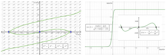  Figure 13. Phase plane diagram (on the left) of the traveling wave system for Equation (36) and the two-dimensional plot (on the right) of the analytic kink type solitary wave solution along with the graph of $f\left(u\right)$ for the case where $D=\beta =\kappa =A=1$ and $B=-1$ at time $t=0$.
• When $\omega =\frac{\kappa }{4A^2}\left(A^2\mathit{D}\kappa -4A^2\beta +3B\mathit{D}\kappa \right)$ and $B=-{\lambda }^2{A}^2$, where a number $\lambda >1$, $f\left(u\right)$ has five real roots, $0,\pm {\lambda }^{-1},$ and $\pm 1$, and hence, $f\left(u\right)$ is a nonlinear function with a strong Allee effect. Consequently, the kink (anti-kink) solution is a solitary wave with asymptotic values of 0 and ${\lambda }^{-1}$ at the left and right infinities. On the other hand, when $\beta =\frac{\mathit{D}\kappa }{4A^2}\left(A^2+3B\right)$, we find $\omega =0$ and thus a standing wave solution exists. Figure 14 shows the phase portraits of the traveling wave system for Equation (36) and the 2-dimensional plot of the analytic kink type solitary wave solutions along with the graph of the proliferation rate $f\left(u\right)$ for the case where $D=\beta =\kappa =A=1$ and $\lambda =4$ at time $t=0$.
  

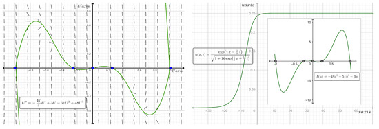  Figure 14. Phase plane diagram (on the left) of the traveling wave system for Equation (36) and the two-dimensional plot (on the right) of the analytic kink type solitary wave solution along with the graph of $f\left(u\right)$ for the case where $D=\beta =\kappa =A=1$ and $\lambda =4$ at time $t=0$.
• When $A=\eta \sqrt{-B}$ and $\omega >\frac{1}{4}\mathit{D}{\kappa }^2-\beta \kappa$, where $\eta =\pm 1$, $f\left(u\right)$ has three real roots, 0 and $\pm 1$, and hence, $f\left(u\right)$ is a nonlinear function with a weak Allee effect. Consequently, the kink (anti-kink) solution is a solitary wave with asymptotic values of 0 and 1 at the left and right infinities. Figure 15 shows the phase portraits of the traveling wave system for Equation (36) and the two-dimensional plot of the analytic kink type solitary wave solutions along with the graph of the proliferation rate $f\left(u\right)$ for the case where $D=\beta =\kappa =\omega =\eta =1$ and $B=-1$ at time $t=0$.
  

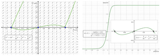  Figure 15. Phase plane diagram (on the left) of the traveling wave system for Equation (36) and the two-dimensional plot (on the right) of the analytic kink type solitary wave solution along with the graph of $f\left(u\right)$ for the case where $D=\beta =\kappa =\omega =\eta =1$ and $B=-1$ at time $t=0$.
• When $\omega =\frac{\kappa }{4A^2{\lambda }^2}\left(A^2{\lambda }^2\mathit{D}\kappa -4A^2{\lambda }^2\beta +3B\mathit{D}\kappa \right)$ and $B=-A^2$, where a number $\lambda >1$, $f\left(u\right)$ has five real roots, $0,\pm {\lambda }^{-1},$ and $\pm 1$, and hence, $f\left(u\right)$ is a nonlinear function with a strong Allee effect. Consequently, the kink (anti-kink) solution is a solitary wave with asymptotic values of 0 and 1 at the left and right infinities. On the other hand, when $\beta =\frac{\mathit{D}\kappa }{4A^2{\lambda }^2}\left(A^2{\lambda }^2+3B\right)$, we find $\omega =0$ and thus, a standing wave solution exists. Figure 16 shows the phase portraits of the traveling wave system for Equation (36) and the two-dimensional plot of the analytic kink type solitary wave solutions along with the graph of the proliferation rate $f\left(u\right)$ for the case where $D=\beta =\kappa =A=1$ and $\lambda =4$ at time $t=0$.
  

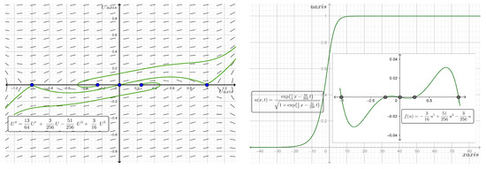  Figure 16. Phase plane diagram (on the left) of the traveling wave system for Equation (36) and the two-dimensional plot (on the right) of the analytic kink type solitary wave solution along with the graph of $f\left(u\right)$ for the case where $D=\beta =\kappa =A=1$ and $\lambda =4$ at time $t=0$.

Moreover, from Equation (36), when $\beta =0$, a solitary wave of the kink (anti-kink) type can be obtained for the reaction–diffusion equation

$$\begin{array}{cc}\hfill & \frac{\partial }{\partial t}u(x,t)-\mathit{D}\frac{{\partial }^2}{\partial x^2}u(x,t)=\hfill \\ & \left(\frac{\beta \kappa +\omega }{4}-\frac{\mathit{D}{\kappa }^2}{16}\right)u(x,t)-\frac{B\left(\mathit{D}{\kappa }^2-\beta \kappa -\omega \right)}{4A^2}{u}^3(x,t)-\frac{3B^2\mathit{D}{\kappa }^2}{16A^4}{u}^5(x,t).\hfill \end{array}$$

(37)

3. Conclusions

We have presented a detailed exposition of a number of traveling wave solutions for a population model in the form of a reaction–diffusion–advection equation. Of particular interest is the influence of the Allee effect on the solution behavior. In Equation (1), $f\left(u\right(x,t\left)\right)$ can be thought of as an instantaneous growth function with an Allee effect. However, some populations may be modeled better, if time delays that could occur from birth to maturation are incorporated into the population model. Recently, a review study [20] looked at time delays introduced into bistable reaction–diffusion systems (similar to a population model with an Allee effect) in the areas of optics and neurobiology. Although, intuitively, one may expect time delays to slow down any moving wave, interestingly, this review study shows how, at times, a large time delay can set a standing wave in motion and can even reverse the direction of movement of the wave at other times. Furthermore, if one is to consider complex media with hereditary, fractal, and non-Markovian properties when modeling population growth with an Allee effect, then one has to consider fractional derivatives [21]. Such a time–fractional reaction–diffusion equation that describes impulse propagation in nerve axons was considered in [21]. By employing a linear stability analysis and numerical computations, this study showed how the fractional order can influence the existence of traveling wave solutions. Another similar study [22] was able to use an interesting transformation to transform a given fractional reaction–diffusion equation into a traditional partial differential equation and then determine the conditions under which traveling wave solutions may or may not exist. The ideas and the methodology presented in this paper could easily be applied to such a transformed traditional partial differential equation. In summary, we have looked at four different forms of the growth function that could be of value to ecologists and environmentalists when deciding on an appropriate growth function for their model in order to study the growth and dispersal of a particular species. Importantly, the traveling waves, given as closed form expressions, will be extremely useful for understanding the spread of invasive species or migration waves in a changing environmental landscape.

References

- Murray, J.D. Mathematical Biology I: An Introduction; Springer: New York, NY, USA, 2002. [Google Scholar]
- Manoranjan, V.S. Bifurcation studies in reaction–diffusion II. J. Comput. Appl. Math. 1984, 11, 307–314. [Google Scholar] [CrossRef]
- Manoranjan, V.S.; Mitchell, A.R.; Sleeman, B.D.; Yu, K.P. Bifurcation studies in reaction–diffusion. J. Comput. Appl. Math. 1984, 11, 27–38. [Google Scholar] [CrossRef]
- Kramer, A.M.; Dennis, B.; Liebhold, A.M.; Drake, J.M. The evidence for Allee effects. Popul. Ecol. 2009, 51, 341–354. [Google Scholar] [CrossRef]
- Fisher, R.A. The wave of advance of advantageous genes. Ann. Eugen. 1937, 7, 355–369. [Google Scholar] [CrossRef]
- Aronson, D.G. Density-dependent interaction-diffusion systems. In Dynamics and Modeling of Reactive Systems, Proceedings of the Advanced Seminar Conducted by the Mathematics Research Center, the University of Wisconsin–Madison, 22–24 October 1979; Academic Press: Cambridge, MA, USA, 1980; pp. 161–176. [Google Scholar]
- Choudhury, S.R. Painlevé analysis and special solutions of two families of reaction-diffusion equations. Phys. Lett. A 1991, 159, 311–317. [Google Scholar] [CrossRef]
- Kolmogorov, A.N.; Petrovskii, I.; Piskunov, N.S. A study of the equation of diffusion with increase in the quantity of matter, and its application to a biological problem. Byul. Mosk. Gos. Univ. 1937, 1, 1–25. [Google Scholar]
- Lu, B.Q.; Xiu, B.Z.; Pang, Z.L.; Jiang, X.F. Exact traveling wave solution of one class of nonlinear diffusion equations. Phys. Lett. A 1993, 175, 113–115. [Google Scholar] [CrossRef]
- Newman, W.I. Some exact solutions to a non-linear diffusion problem in population genetics and combustion. J. Theor. Biol. 1980, 85, 325–334. [Google Scholar] [CrossRef] [PubMed]
- Zhang, H. New application of the -expansion method. Commun. Nonlinear Sci. Numer. Simul. 2009, 14, 3220–3225. [Google Scholar] [CrossRef]
- Alzaleq, L.; Alzaalig, A.; Manoranjan, V. Exact traveling waves for a generalized Fisher’s equation. J. Interdiscip. Math. 2022, 25, 1201–1220. [Google Scholar] [CrossRef]
- FitzHugh, R. Impulses and physiological states in theoretical models of nerve membrane. Biophys. J. 1961, 1, 445–466. [Google Scholar] [CrossRef]
- Alzaleq, L.; Manoranjan, V. Analysis of the Fisher-KPP equation with a time-dependent Allee effect. IOP Scinotes 2020, 1, 025003. [Google Scholar] [CrossRef]
- Manoranjan, V.; Alzaleq, L. Analysis of a population model with advection and an autocatalytic-type growth. Int. J. Biomath. 2022, 16, 2250078. [Google Scholar] [CrossRef]
- Bani-Yaghoub, M.; Yao, G.; Voulov, H. Existence and stability of stationary waves of a population model with strong Allee effect. J. Comput. Appl. Math. 2016, 307, 385–393. [Google Scholar] [CrossRef]
- Fadai, N.T.; Simpson, M.J. Population dynamics with threshold effects give rise to a diverse family of Allee effects. Bull. Math. Biol. 2020, 82, 1–22. [Google Scholar] [CrossRef] [PubMed]
- Alzaleq, L.; Manoranjan, V. An Energy Conserving Numerical Scheme for the Klein–Gordon Equation with Cubic Nonlinearity. Fractal Fract. 2022, 6, 461. [Google Scholar] [CrossRef]
- Alzaleq, L.; Manoranjan, V.; Alzalg, B. Exact traveling waves of a generalized scale-invariant analogue of the Korteweg–de Vries equation. Mathematics 2022, 10, 414. [Google Scholar] [CrossRef]
- Rombouts, J.; Gelens, L.; Erneux, T. Travelling fronts in time-delayed reaction–diffusion systems. Philos. Trans. R. Soc. A 2019, 377, 20180127. [Google Scholar] [CrossRef] [PubMed]
- Datsko, B.; Gafiychuk, V.; Podlubny, I. Solitary travelling auto-waves in fractional reaction–diffusion systems. Commun. Nonlinear Sci. Numer. Simul. 2015, 23, 378–387. [Google Scholar] [CrossRef]
- Zheng, B.; Kai, Y.; Xu, W.; Yang, N.; Zhang, K.; Thibado, P.M. Exact traveling and non-traveling wave solutions of the time fractional reaction–diffusion equation. Phys. A Stat. Mech. Appl. 2019, 532, 121780. [Google Scholar] [CrossRef]
Disclaimer/Publisher’s Note: The statements, opinions and data contained in all publications are solely those of the individual author(s) and contributor(s) and not of MDPI and/or the editor(s). MDPI and/or the editor(s) disclaim responsibility for any injury to people or property resulting from any ideas, methods, instructions or products referred to in the content. |
© 2023 by the authors. Licensee MDPI, Basel, Switzerland. This article is an open access article distributed under the terms and conditions of the Creative Commons Attribution (CC BY) license (https://creativecommons.org/licenses/by/4.0/).