Abstract
Identifying the mutational processes that shape the nucleotide composition of the mitochondrial genome (mtDNA) is fundamental to better understand how these genomes evolve. Several methods have been proposed to analyze DNA sequence nucleotide composition and skewness, but most of them lack any measurement of statistical support or were not developed taking into account the specificities of mitochondrial genomes. A new methodology is presented, which is specifically developed for mtDNA to detect compositional changes or asymmetries (AT and CG skews) based on nonparametric regression models and their derivatives. The proposed method also includes the construction of confidence intervals, which are built using bootstrap techniques. This paper introduces an R package, known as seq2R, that implements the proposed methodology. Moreover, an illustration of the use of seq2R is provided using real data, specifically two publicly available complete mtDNAs: the human (Homo sapiens) sequence and a nematode (Radopholus similis) mitogenome sequence.
Keywords:
R package; nonparametric model; multiple change points; bootstrap techniques; DNA compositional analysis MSC:
62G05; 62P10
1. Introduction
Understanding how the mitochondrial genome (mtDNA) evolves and replicates is crucial for advancing our knowledge of diseases and disorders, evolutionary relationships, and important cell functions. Although the exact mechanism of mtDNA replication is still not fully understood, it is an active area of research [1,2]. Two competing modes of mtDNA replication exist: the strand-displacement model and the strand-coupled model. The strand-displacement model requires two defined origins of replication; therefore, one strand is highly exposed to mutation, leading to a strong nucleotide compositional bias that may change near replication origins/termini. Comparative genomic studies using invertebrate [3,4,5,6] and vertebrate [7,8] mitogenomes support this model. In the strand-coupled model, both strands replicate symmetrically and in a coordinated manner, with only one origin/terminus needed due to the circular nature of mtDNA. Notably, this model does not produce strong nucleotide compositional biases or abrupt changes.
Over the years, various compositional analyses have been conducted to identify the location of change points in the nuclear genomes of major taxonomic groups, such as bacteria [9] or eukaryotic species [10]. A change point is defined as a region in the DNA sequence where there is a change in the proportion of nucleotides (the building blocks that make up DNA). This change can be due to mutations during replication, transcription, or DNA repair [11]. If these mutations occur during the replication process, it is expected that large changes in the nucleotide composition will appear at replication origins and at the terminus. Therefore, identifying these change points will allow us to determine, for example, the location of replication origins/termini.
Little attention has been focused on analyzing the nucleotide composition asymmetries of organelle mitogenomes. The methods that were originally developed for bacterial or nuclear genomes are not optimal for mtDNA analysis due to the much smaller size of mtDNA sequences. For example, animal mtDNA is typically around 17 kilo base pairs (kbp), which is approximately 76 times smaller than a small bacterial genome of 1.3 mega base pairs (Mbp) and 2700 times smaller than the smallest human chromosome. Therefore, these methods are not well-suited for analyzing mtDNA sequences, and the expected amount of information and resolution (e.g., window size or step) may also pose a challenge in applying them to mtDNA analysis.
Some tools and methods have been used for mtDNA analysis. For instance, there are readily available tools (such as online tools or R/Python packages) that are easy to use, such as skew analyses [12,13,14] and DNA-Walk [15]. However, these tools do not have statistical tests to support their findings. In contrast, some published methods have statistical tests to support their inferences/findings [16,17], but they are not implemented in any online tool or in a function/package of a statistical language such as R [18]. Our package aims to address this gap by providing statistical methods specifically developed for mtDNA analysis that are available as a freely downloadable R package.
Identifying compositional change points in a statistical framework can be a challenging task. Numerous methodological approaches have been developed to analyze change point models, i.e., Bayesian estimation [19], maximum likelihood estimation [20,21], least squares regression [22] or nonparametric regression [23,24,25,26]. These methodologies can be applied in many different areas, including in the context of modeling DNA sequences [27,28]. To facilitate the use of these statistical methodologies, freely available software such as R packages has been released in the past decade, including DNAcopy [29] based on the recursive circular binary segmentation algorithm [20]; strucchange [30], which has a dynamic programming algorithm [22]; cpm for online change point detection; seqinr [31], which is devoted to the retrieval and analysis biological sequences; and the bcp package [32,33], which implements a Bayesian change point procedure proposed by Barry and Hartigan [34].
There are other R packages available on CRAN for detecting change points in other application contexts, such as time series analysis. Killick and Eckley [35] developed the changepoint R package, which provides multiple change point search methods, such as segment neighborhood, binary segmentation, and the Pruned Exact Linear Time (PELT) algorithm, which can be used in conjunction with a variety of test statistics. An extended version of the PELT algorithm with nonparametric cost functions was implemented by Haynes [36] in the changepoint.np package. More recently, the R package mosum was implemented with mathematically well-justified procedures for the multiple mean change problem using moving sum statistics [37], as well as the bootstrap procedure, to generate confidence intervals for the location of change points. However, none of the existing R packages analyzes the nucleotide composition asymmetries of mtDNA.

Table 1.
Comparison of methodologies described in the literature in a biological framework.
Table 2.
Comparison of some well-known R packages for change point detection described in the literature.
Part of our philosophy is to facilitate the usage of new statistical methodology by the scientific community. With that in mind, we implemented a methodology in seq2R [39], a user-friendly and simple R package that identifies and locates compositional change points in DNA sequences by fitting nonparametric regression models and their first derivatives. Since the estimation procedure of this methodology for large datasets implies a high computational cost, Fortran (FORmula TRANslation) [40] was used as the programming language. Our approach to detecting significant features of the curves, such as critical points, is based on detecting the maximum or minimum of the first derivative of nonparametric regression models with binary response. To estimate the regression curve and its first derivative, we applied local linear kernel smoothers [41]. Additionally, smoothing windows are automatically selected using a cross-validation technique [42]. Inference procedures imply the construction of confidence intervals, which can be obtained by bootstrap methods [43,44]. The choice of smoothing windows and the usage of bootstrap resampling techniques may entail high computational costs. To considerably reduce computation time and render the operational procedures, binning techniques are applied [45].
In this article, in addition to the developed methodology, we explain and illustrate how numerical and graphical output for all methods can be obtained using the seq2R package. Although the proposed methods can be used with all kinds of genomic sequences, two mitochondrial genomes (mitogenomes) were chosen to illustrate the package with real data.
The remainder of this paper is organized as follows. In Section 2, the estimation procedure of the DNA compositional change point detection and the bootstrap method are described. The functions programmed in seq2R are explored in Section 3. Two practical examples using two DNA sequences (mitogenomes) to illustrate how the package can be applied, as well as its performance, are presented in Section 4. Finally, in Section 5, we briefly present the conclusions of this paper.
2. Nonparametric Estimation Procedures
It is well-known that a DNA sequence is a long chain made up of repeating units called nucleotides, which include adenine, thymine, cytosine, and guanine nucleotides. In order to analyze a DNA sequence, it is necessary to convert it into four binary variables (C, G, A, and T). We define C as a Bernoulli variable, where the value 1 represents the presence of the cytosine nucleotide at a specific position (X) of the sequence, and the value 0 represents its absence. The three other variables can be obtained similarly.
To study the nucleotide composition and detect possible change points in the sequence, it is possible to consider the skew or skew [46]. Both skews measure deviations in the amount of one nucleotide compared to another, and they are calculated for a given X values as follows:
and
where , , , and are the probabilities of the appearance of cytosine, guanine, adenine, and thymine, respectively.
The proposed skews allow us to determine whether the relationship between pairs of nucleotides is altered. In the case of a change, for example, in the number of cytosines, the value of the skew increases considerably, which is reflected in the estimated curve. Taking this into account, the use of derivatives is of great help in this context, specifically for estimating the point where the first derivative of is maximum or minimum, which corresponds to a critical point in the trend of the estimated skew (). This point reflects a change or deviation in the relationship between the two nucleotides.
For simplicity, we will only present the methodology for calculating the skew, as the skew can be obtained in a similar way. To obtain the aforementioned skew, it is necessary to estimate the probabilities and . To achieve this, we used the nonparametric logistic regression models:
and
where and are unknown functions. As described in the Section 2.1, we used a combination of the local scoring algorithm [47] and local linear kernel smoothers [41] to estimate these probabilities, taking into account the computational cost (see Section 2.2). Additionally, this estimation procedure allows us to obtain the first derivative of and . After obtaining and according to the models in (3) and (4), it is possible to calculate the skew by inserting the estimated probabilities into (1). Furthermore, we can obtain the first derivative of this skew, .
At this point, it is essential to emphasize that we are focused on identifying change points of the skew curve in DNA sequences. For our purposes, we refer to these points as inflection points, where the first derivative of the skew curve reaches a maximum or minimum. To make inferences about these points, we need to construct confidence intervals for the first derivative of the skew curve. We construct these intervals using binary bootstrap techniques (for more details, see Section 2.3).
Finally, the procedure to detect the critical points is based on the following steps: (i) locating the regions at the sequence (X values) where the confidence interval of the first derivative of the skew does not contain the value zero; then, (ii) for each region, determining the critical point as the maximizer or minimizer of
where is a very fine grid of B equidistant points in a range of X values corresponding to the previously bounded region.
2.1. Estimation of the Logistic Model—The Local Scoring Algorithm
Let be a random sample of of size n (total length of DNA sequence), where Y could be any of the cited binary variables (C, G, A, or T). The estimation of , , , and is based on the use of the local scoring algorithm with local linear kernel smoothers. For simplicity, we show the procedure for obtaining . The steps of the algorithm that enables estimation of the model in (3) are as follows:
Initialize. Compute the initial estimates, and ().
Step 1. Form the adjusted dependent variables and the weights ,
The estimation of () and its first derivative () at a position (x) is defined as
where the vector is the minimizer of
where K denotes a kernel function (normally, a symmetric density), and is the smoothing parameter or bandwidth. Commonly used kernel functions include the uniform , the Epanechnikov , the triweight kernel function , and the Gaussian kernel , which was used in this work.
Step 2. Repeat Step 1., with being replaced by
where is a small threshold (by default, ), and
The obtained nonparametric estimates of and are known to heavily depend on the bandwidth (h). Various proposals based on some error criterion for optimal selection have been suggested. However, due to the difficulty of asymptotic theory, optimal selection remains a challenging open problem. As a practical solution to this problem, in this paper, we consider that the smoothing bandwidth (h) can be selected automatically by minimizing the following weighted cross-validation error criterion:
where is a set of weights, and indicates the fit at , leaving out the i-th data point based on the smoothing parameter (h). Note that this bandwidth selection procedure is performed for each iteration of Step 1.
2.2. Computational Aspects
It should be noted here that the computational cost involved in the choice of smoothing the bandwidth and the construction of bootstrap confidence intervals can be considerably reduced by using binning-type acceleration techniques. Linear binning is described in detail in [45]. Briefly, the binning sample () and the weights () are constructed, where is a grid of equidistant points along range X,
where , and denotes the distance between two consecutive nodes. The binning approximation of the estimator in (5) is obtained by minimizing the following expression
Furthermore, the cross-validation error given in (6) can be approximated by
where is the estimate obtained without the r-th node of the binning sample. This approximation reduces the computation time considerably, since the calculation of CV only requires kernel K to be assessed at a maximum N points for each choice of bandwidth (h), and for these purposes, nodes with null weight are not taken into account.
The choice of the number of nodes is therefore a tradeoff between approximation error and computational speed; the finer the grid of chosen points, the better the binning approximations.
2.3. Percentile Bootstrap Confidence Intervals
Once the estimated curves have been obtained, it is necessary to construct confidence intervals in order to make inferences about certain of their features. These intervals can be obtained based on the estimates of and and are useful in different contexts: (i) to determine whether the estimate of the skew at a particular point differs from zero and (ii) to approximate the sought change points. Because of the nature of the dataset, the percentile bootstrap procedure was used to construct these confidence intervals. For instance, the confidence interval for the estimated skew () can be obtained as follows:
Step 1. Obtain the estimates of the mean conditional and by fitting the model in (3) and obtain the skew. We know that the sum of these probabilities may not be equal to one, although it should be close. For this reason, we rescale them to ensure that they sum up to one.
Step 2. For (i.e., B = 1000), generate bootstrap samples , where the bootstrap response variables () are distributed in accordance with , where , and calculate the skew. The limits for the confidence interval of the skew are given by
where represents the p-percentile of values.
3. Package Description
As mentioned in Section 2, the seq2R package includes an algorithm for analyzing asymmetries based on the nucleotide composition of DNA sequences. This package is useful for loading various types of files commonly used for importing biological sequences, as well as retrieving sequences from the GenBank (Managed by the NCBI, National Center for Biotechnology Information, formerly at Los Alamos.)dataset.
Additionally, seq2R allows for inference about change points related to the derivative curves, such as maximum or minimum points. This software is designed to be used with the R statistical program [18]. In R, programming is based on objects, and computations are performed using specialized functions designed for specific calculations. Our package consists of seven functions that enable users to apply the methodology. A summary of these functions is provided in Table 3.
Table 3.
Summary of functions in the seq2R package.
It should be noted that any sequence must be read by read.genbank or read.all before proceeding. After this step, the character vector needs to be converted into binary code using transform. At this point, users can fit and illustrate the models and methods discussed in the previous section using two functions: find.points and plot. Table 4 and Table 5 provide a summary of the arguments for these two functions. Finally, if one wants to determine the change points, i.e., the positions in the sequence that maximize or minimize the first derivative of the skew curves, the critical function can be used to obtain them.
Table 4.
Summary of the arguments for the find function.
Table 5.
Summary of the arguments of the plot function.
4. Application to Real Data
The methodology described in Section 2 was used to estimate the and skew profiles and determine the compositional change points in two mitochondrial genomes (mitogenomes)—the human and nematode mitogenomes (NCBI accession numbers NC_012920 and NC_013253, respectively)—using the seq2R package.
The exact mechanism of mitochondrial DNA replication in mammals, including the human mitogenome, has been a matter of controversy in the last decade [49,50]. The classical model of mitogenome replication, which suggests the existence of two different replication origins [51], has been challenged with the proposal of alternative models that only consider one origin of replication [52,53].
The first objective of our methodology applied to the human mitogenome was to determine the number of replication origins and hypothesize which replication model is supported by our results. Second, we used the nematode mitogenome of the species Radopholus similis to compare our methodology’s results with those of another commonly used approach that lacks statistical testing and relative nucleotide rates (T+G/A+C, G/A, and T/C) [13]. Our goal was to demonstrate that identifying compositional change points can improve our understanding of the replication process in these mitogenomes. However, it should be noted that the methodology is not limited to detecting replication origins or termini; other processes such as transcription, selection, or recombination can also cause compositional changes. Therefore, all results should be interpreted with caution. Our methodology can be applied to all types of genomic sequences.
In the following section, we provide details on how to call functions and R commands of seq2R, which can be loaded into R using library(seq2R).
4.1. Human Mitogenome (Homo sapiens)
We can use the function read.genbank to retrieve the human mitochondrial sequence from the GenBank database. Below is an excerpt of this character vector
> library(seq2R)
> mtDNAhuman <- read.genbank("NC_012920")
> mtDNAhuman
[[1]]
[1] "g" "a" "t" "c" "a" "c" "a" "g" "g" "t" "c" "t" "a" "t" "c" "a"
[17] "c" "c" "c" "t" "a" "t" "t" "a" "a" "c" "c" "a" "c" "t" "c" "a"
[33] "c" "g" "g" "g" "a" "g" "c" "t" "c" "t" "c" "c" "a" "t" "g" "c"
[49] "a" "t" "t" "t" "g" "g" "t" "a" "t" "t" "t" "t" "c" "g" "t" "c"
…
[[2]]
[1] "NC_012920"
attr(,"species")
[1] "Homo_sapiens"
To begin the analysis, it is necessary to convert our sequence into binary variables, where a value of 1 denotes the presence of a nucleotide at position X in the sequence, while 0 indicates the absence of a nucleotide. To do this, the following input command should be typed
> DNA <- transform(mtDNAhuman)
> DNA
$AT
$AT[[1]]
X A T
[1,] 2 1 0
[2,] 3 0 1
[3,] 5 1 0
[4,] 7 1 0
…
$CG
$CG[[1]]
X C G
[1,] 1 0 1
[2,] 4 1 0
[3,] 6 1 0
[4,] 8 0 1
…
To carry out compositional analyses, we used the following main function
> seq1 <- find.points(DNA)
Results are printed on the screen using
> seq1
Call:
find.points(x = DNA)
Number of A-T base pairs:9218
Number of C-G base pairs:7350
Number of binning nodes: 300
Number of bootstrap repeats: 100
Bandwidth: 0.5862069 0.1379310
Exists any critical point? TRUE
It should be noted that there is at least a critical point, as shown in the last logical argument of this short summary. To illustrate where the critical point is, seq2R package also provides plots for the analyses of the skews. First, the estimate of skew and its first derivative are displayed in Figure 1 (upper and lower panel, respectively) with 95% bootstrap confidence intervals. These plots can be obtained with the following command:
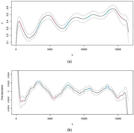
Figure 1.
Human mitogenome. (a) Regression curve for the skew profile (solid lines) with bootstrap-based 95% confidence intervals (dashed lines). Red line: X variable points that minimize the first derivative. Blue line: X variable points that maximize the first derivative. (b) First derivative for the skew profile (solid lines) with bootstrap-based 95% confidence intervals (dashed lines). Red and blue lines as mentioned before.
> plot(seq1, der = 0, base.pairs = "CG", CIcritical = TRUE,
ylim = c(0.08,0.67))
> plot(seq1, der = 1, base.pairs = "CG", CIcritical = TRUE,
ylim = c(-0.0005,0.00045))
At this point, a main question that arises is: What are the positions of the detected change points in our sequence? To answer this, we used the following input commands.
> critical(seq1, base.pairs = "CG")
Critical Low_CI Up_CI
[1,] 721.3478 499.7023 1275.462
[2,] 3325.6823 2966.8935 3713.562
[3,] 5542.1371 5127.9370 5845.514
[4,] 7647.7692 7041.0144 8091.060
[5,] 10861.6288 10639.9833 11027.863
[6,] 13465.9632 12801.0268 14020.077
[7,] 15017.4816 14878.9532 15622.851
From the compositional analyses of the human mitogenome specifically focusing on the content, we made the following observations: the two typical origins of replication, OH and OL, are located in regions where critical points were also identified (indicated by red lines in Figure 1). In the human mitogenome, OL is a very small genomic region located at positions 5730 to 5760. Interestingly, one of the critical points identified in the analysis is located precisely in that same region. Additionally, the OH, located at the beginning (1–576) and terminus (16,024–16,569) of the genomic sequence, was also identified in our analysis.
Secondly, for the analyses, we can obtain the estimated curve and its first derivative with 95% bootstrap confidence intervals in the same way as for the skew (Figure 2, upper and lower panel, respectively). Additionally, we can locate the change points using the same approach as for the analysis.
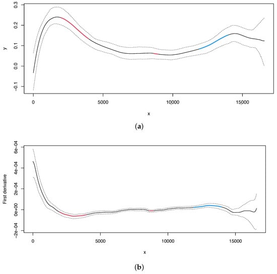
Figure 2.
Human mitochondrial DNA. (a) Regression curve for the skew profile (solid lines) with bootstrap-based 95% confidence intervals (dashed lines). Red line: X variable points that minimize the first derivative. Blue line: X variable points that maximize the first derivative. (b) First derivative for the skew profile (solid lines) with bootstrap-based 95% confidence intervals (dashed lines). Red and blue lines as mentioned before.
> plot(seq1, der = 0, base.pairs = "AT", CIcritical = TRUE)
> plot(seq1, der = 1, base.pairs = "AT", CIcritical = TRUE)
> critical(seq1, base.pairs = "AT")
Critical Low_CI Up_CI
[1,] 3049.258 1996.569 3963.435
[2,] 8755.940 8645.130 8922.154
[3,] 13077.505 11914.007 13963.980
Additionally, the analysis (Figure 2) appears to detect alternative origins of replication: one in the region upstream to the OL (i.e., before position 5000) and another one around position 15,000. The latter inferred OL (around position 15,000) may be homologous to the OL recently mapped in the mouse mitogenome [54]. If the identified compositional bias reflects the replication process and if the change points correspond to the origins of replication, it is possible that more than one replication mechanism (using different origins of replication) may exist in the human mitogenome, since we find evolutionary signatures of more than one potential mechanism. Indeed, the most recent biochemical findings support this hypothesis [55,56].
4.2. Nematode Mitogenome (Radopholus similis)
Nematodes, or roundworms, are a highly diverse phylum of animals. While some species are free-living, others are parasitic and responsible for causing diseases in both animals and plants. The nematode mitogenome analyzed in this study is plant-parasitic. However, little is known about its replication mechanism. Compositional analyses of the relative amounts of T and G versus A and C reveal a pattern consistent with the existence of two different replication origins [13] located around positions 4100 and 11,000. Additionally, the authors of [13] highlighted a compositional change after position 1000, which was suggested to be related to the replication mechanism but did not correspond to a replication origin. Instead, it was caused by a collision between DNA polymerases during mitogenome replication [13].
We can obtain the nematode mitogenome from the GenBank dataset with accession number NC_013253. Below is an excerpt of this sequence. We convert our character vector into binary variables and then calculate the estimates of the skew profile using the following input commands:
> library(seq2R)
> nematode <- read.genbank("NC_013253")
[[1]]
[1] "t" "a" "a" "a" "g" "a" "a" "a" "a" "t" "a" "t" "t" "t" "t" "a"
[17] "a" "t" "t" "t" "t" "a" "g" "a" "a" "t" "g" "t" "t" "t" "c" "a"
[33] "t" "t" "g" "t" "t" "a" "a" "t" "g" "a" "a" "a" "a" "g" "g" "t"
[49] "t" "t" "t" "t" "t" "c" "t" "t" "t" "g" "a" "t" "a" "t" "t" "a"
…
[[2]]
[1] "NC_013253"
attr(,"species")
[1] "Radopholus_similis"
> nem <- transform(nematode)
> (seq2<-find.points(nem, kbin = 450, n.bandwidths = 10))
Call:
find.points(x = nem, kbin = 450, n.bandwidths = 10)
Number of A-T base pairs:14340
Number of C-G base pairs:2451
Number of binning nodes: 450
Number of bootstrap repeats: 100
Bandwidth: 0.3333333 0.8888889
Exists any critical point? TRUE
For illustration purposes, we report the estimate and its first derivative of the skew with 95% bootstrap confidence intervals (Figure 3). The change points values with 95% bootstrap confidence intervals are shown by typing the following code.
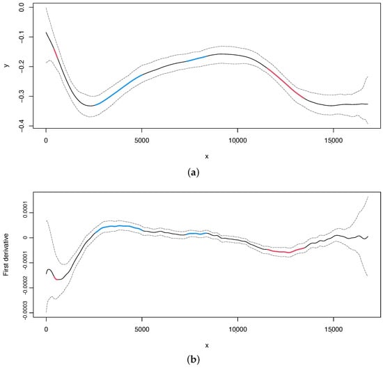
Figure 3.
Nematode mitochondrial DNA. (a) Regression curve for the skew profile (solid lines) with bootstrap-based 95% confidence intervals (dashed lines). Red line: X variable points that minimize the first derivative. Blue line: X variable points that maximize the first derivative. (b) First derivative for the skew profile (solid lines) with bootstrap-based 95% confidence intervals (dashed lines). Red and blue lines as mentioned before.
For illustrative purposes, we report the estimate and first derivative of the skew, along with 95% bootstrap confidence intervals, in Figure 3. The values of change points, along with their 95% bootstrap confidence intervals, can be obtained by using the following code:
> par(mfrow=c(2,1))
> plot(seq2, der = 0, base.pairs = "AT", CIcritical = TRUE)
> plot(seq2, der = 1, base.pairs = "AT", CIcritical = TRUE,
ylim = c(-0.0002,0.0002))
> critical(seq2, base.pairs = "AT")
Critical Low_CI Up_CI
[1,] 561.5676 169.1703 561.5676
[2,] 3756.8030 2579.6110 4596.2530
[3,] 8325.4290 7891.6898 8325.4290
[4,] 12669.8280 11662.2076 13495.9646
In the case of skew, we can obtain the estimated curve and its first derivative with 95% bootstrap confidence intervals in the same way as for the skew (Figure 4, upper and lower panel, respectively). Our method can detect two change points at positions 4264 and 11,186, which overlap with the change points located in the skew, as also reported in [13].
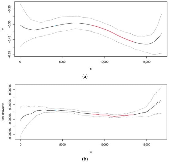
Figure 4.
Nematode mitochondrial DNA. (a) Regression curve for the skew profile (solid lines) with bootstrap-based 95% confidence intervals (dashed lines). Red line: X variable points that minimize the first derivative. (b) First derivative for the skew profile (solid lines) with bootstrap-based 95% confidence intervals (dashed lines). Red line as mentioned before.
> par(mfrow = c(2,1))
> plot(seq2, der = 0, base.pairs = "CG", CIcritical = TRUE)
> plot(seq2, der=1, base.pairs = "CG", CIcritical = TRUE)
> critical(seq2, base.pairs = "CG")
Critical Low_CI Up_CI
[1,] 4264.553 4124.436 4264.553
[2,] 11186.326 8524.105 13456.219
After applying our methodology to this nematode mitogenome, we were able to identify three significant change points, which correspond to the three points highlighted in [13]. Therefore, we not only confirmed the presence of change points related to the replication process but also provided statistical support and confidence intervals for their location.
4.3. Computational Times
As we mentioned previously, the proposed methodology can be used not only with mitogenomes but also with other types of genomic sequences. To compare its performance, we analyzed different genomic sequences in terms of the time required for analysis.
To compare the performance of the proposed methodology, larger genomic sequences than the human mitogenome analyzed in Section 4.1 were chosen, starting from approximately 16 kbp and increasing by a factor of 10 for each subsequent genomic sequence up to approximately 13 Mbp (Table 6). As the length of the sequence determines the computational cost, analyzing some larger genomic sequences may require an infeasible processing time. Table 6 shows the execution time (in minutes) for different species, types, and lengths of sequences (in base pairs) when the proposed methodology is run on an Apple Macbook Pro M1 with eight cores, 16 GB of RAM, and an onboard SSD. As expected, the computational time increases with sequence length. Results show that our proposed methodology can handle the analysis of any sequence size, although the computational burden is high for the Sorangium cellulosum bacterial genome.
Table 6.
Computational times (in minutes) for different species, types, and lengths of sequences (in base pairs).
4.4. Compositional Analysis with Another R Package: Seqinr
The aim of this section is to compare our results with those obtained using the seqinr R package, which is considered the most complete R package for genomic sequence analysis and nucleotide compositional analysis. To accomplish this, we analyzed the same mitogenomes as in the previous subsections (human and nematode sequences, as discussed in Section 4.1 and Section 4.2, respectively) using seqinr.
Here, we focus our discussion on the change points associated with the origins of replication. In the human mtDNA, two origins of replication were identified—one for each complementary strand. The first is located around position 5730, and the other is in the major non-coding region located at the beginning and the end of the circular genome (joining the start of the genome (positions 1 to 576) with the end of the genome (positions 16,024 to 16,569)). As we mentioned before, our method is able to detect change points that overlap with these two origins of replication; in fact, the lower limit of the confidence intervals of the first skew critical point overlaps with the major non-coding region. In addition, the third skew change point includes the other origin of replication.
After applying the seqinr to this human sequence, it is possible to associate a minor change detected near position 6000 with the first origin of replication. However, the method is not able to detect the other origin of replication at the start/end of the genome because, as mentioned in Table 2, this analysis can only be performed in coding regions (i.e., regions of protein-coding genes), but this origin of replication is located in a major non-coding region.
The nematode genome has three major change points located at positions 1100, 4100, and 11,100, with the last two identified as the two origins of replication found in this genome [13]. Our method is able to detect change points that overlap with the replication origins. Specifically, the confidence intervals of the second skew change point contain the change point around position 4100 but miss the other change point/replication origin by approximately 500 nucleotides. Interestingly, these two change points are detected by the skew analysis, with two critical points identified at position 4264 (the confidence interval of which contains the position 4100) and 11,186. In contrast, the cumulative composite skew index analysis using seqinr fails to detect any of the change points associated with the origins of replication.
Overall, it seems that our method shows good performance in the identification of change points associated with the origins of replication, unlike seqinr, which, in these examples, misses some of them.
5. Conclusions
In this paper, we discussed the implementation of a new method to detect change points in DNA sequences using the seq2R package in R. The advantage of using R is its excellent statistical and graphical capabilities. The package includes a local scoring algorithm based on local linear kernel smoothers. While the methodology was illustrated using mitochondrial genomes, it can be applied to any type of DNA sequence. However, complete DNA sequences such as chromosomes may require considerable computational time, which was addressed by implementing Fortran functions.
The seq2R package is available on the Comprehensive R Archive Network. The proposed method aims to provide a user-friendly, fully automated, and reproducible approach to change point detection with statistical support for genomic analysis.
Author Contributions
Conceptualization, N.M.V., M.S., M.M.F. and J.R.-P.; methodology, N.M.V., M.S. and J.R.-P.; software, N.M.V. and M.S.; formal analysis, N.M.V., M.S., M.M.F. and J.R.-P.; original draft preparation, N.M.V., M.S., M.M.F. and J.R.-P.; review and editing, N.M.V. and M.S.; supervision, N.M.V. and M.S.; All authors have read and agreed to the published version of the manuscript.
Funding
This research was funded by the Spanish Ministry of Science and Innovation (FEDER support included) as part of projects MTM2011-23204 and PID2020-118101GB-I00 and by Xunta de Galicia from 10PXIB 300 068 PR.
Data Availability Statement
The seq2R package is freely available on 20 April 2023 from CRAN at https://CRAN.R-project.org/package=seq2R. A manual of its use in practice is also available, and complete genomes can be found at https://pubmed.ncbi.nlm.nih.gov/.
Conflicts of Interest
The authors declare no conflict of interest.
Abbreviations
The following abbreviations are used in this manuscript:
| DNA | Deoxyribonucleic acid |
| mtDNA | Mitochondrial DNA |
| PELT | Pruned Exact Linear Time algorithm |
| Fortran | FORmula TRANslation |
References
- Touchon, M.; Nicolay, S.; Audit, B.; Brodie of Brodie, E.B.; d’Aubenton Carafa, Y.; Arneodo, A.; Thermes, C. Replication-associated strand asymmetries in mammalian genomes: Toward detection of replication origins. Proc. Natl. Acad. Sci. USA 2005, 102, 9836–9841. [Google Scholar] [CrossRef] [PubMed]
- Matkarimov, B.T.; Saparbaev, M.K. DNA Repair and Mutagenesis in Vertebrate Mitochondria: Evidence for Asymmetric DNA Strand Inheritance. In Mechanisms of Genome Protection and Repair; Zharkov, D.O., Ed.; Springer International Publishing: Cham, Switzerland, 2020; pp. 77–100. [Google Scholar]
- Hassanin, A.; Léger, N.; Deutsch, J. Evidence for Multiple Reversals of Asymmetric Mutational Constraints during the Evolution of the Mitochondrial Genome of Metazoa, and Consequences for Phylogenetic Inferences. Syst. Biol. 2005, 54, 277–298. [Google Scholar] [CrossRef] [PubMed]
- Wei, S.J.; Shi, M.; Chen, X.X.; Sharkey, M.J.; van Achterberg, C.; Ye, G.Y.; He, J.H. New Views on Strand Asymmetry in Insect Mitochondrial Genomes. PLoS ONE 2010, 5, e12708. [Google Scholar] [CrossRef] [PubMed]
- Jakovlić, I.; Zou, H.; Zhao, X.M.; Zhang, J.; Wang, G.T.; Zhang, D. Evolutionary history of inversions in directional mutational pressures in crustacean mitochondrial genomes: Implications for evolutionary studies. Mol. Phylogenet. Evol. 2021, 164, 107288. [Google Scholar] [CrossRef]
- Ghiselli, F.; Gomes-dos Santos, A.; Adema, C.M.; Lopes-Lima, M.; Sharbrough, J.; Boore, J.L. Molluscan mitochondrial genomes break the rules. Philos. Trans. R. Soc. B Biol. Sci. 2021, 376, 20200159. [Google Scholar] [CrossRef]
- Fonseca, M.M.; Posada, D.; Harris, D.J. Inverted Replication of Vertebrate Mitochondria. Mol. Biol. Evol. 2008, 25, 805–808. [Google Scholar] [CrossRef]
- Stewart, J.B.; Chinnery, P.F. Extreme heterogeneity of human mitochondrial DNA from organelles to populations. Nat. Rev. Genet. 2021, 22, 106–118. [Google Scholar] [CrossRef]
- Hubert, B. SkewDB, a comprehensive database of GC and 10 other skews for over 30,000 chromosomes and plasmids. Sci. Data 2022, 9, 92. [Google Scholar] [CrossRef]
- Dao, F.Y.; Lv, H.; Zulfiqar, H.; Yang, H.; Su, W.; Gao, H.; Ding, H.; Lin, H. A computational platform to identify origins of replication sites in eukaryotes. Briefings Bioinform. 2020, 22, 1940–1950. [Google Scholar] [CrossRef]
- Frank, A.; Lobry, J. Asymmetric substitution patterns: A review of possible underlying mutational or selective mechanisms. Gene 1999, 238, 65–77. [Google Scholar] [CrossRef]
- Grigoriev, A. Analyzing genomes with cumulative skew diagrams. Nucleic Acids Res. 1998, 26, 2286–2290. [Google Scholar] [CrossRef]
- Jacob, J.; Vanholme, B.; Van Leeuwen, T.; Gheysen, G. A unique genetic code change in the mitochondrial genome of the parasitic nematode Radopholus similis. BMC Res. Notes 2009, 2, 192. [Google Scholar] [CrossRef]
- Reyes, A.; Gissi, C.; Pesole, G.; Saccone, C. Asymmetrical directional mutation pressure in the mitochondrial genome of mammals. Mol. Biol. Evol. 1998, 15, 957–966. [Google Scholar] [CrossRef] [PubMed]
- Brugler, M.; France, S. The Mitochondrial Genome of a Deep-Sea Bamboo Coral (Cnidaria, Anthozoa, Octocorallia, Isididae): Genome Structure and Putative Origins of Replication Are Not Conserved Among Octocorals. J. Mol. Evol. 2008, 67, 125–136. [Google Scholar] [CrossRef] [PubMed]
- Faith, J.J.; Pollock, D.D. Likelihood analysis of asymmetrical mutation bias gradients in vertebrate mitochondrial genomes. Genetics 2003, 165, 735–745. [Google Scholar] [CrossRef] [PubMed]
- Rodakis, G.; Cao, L.; Mizi, A.; Kenchington, E.; Zouros, E. Nucleotide Content Gradients in Maternally and Paternally Inherited Mitochondrial Genomes of the Mussel. J. Mol. Evol. 2007, 65, 124–136. [Google Scholar] [CrossRef] [PubMed]
- R Development Core Team. R: A Language and Environment for Statistical Computing; R Foundation for Statistical Computing: Vienna, Austria, 2022; ISBN 3-900051-07-0. [Google Scholar]
- Bacon, D.W.; Watts, D.G. Estimating the transition between two intersecting straight lines. Biometrika 1971, 58, 525–534. [Google Scholar] [CrossRef]
- Olshen, A.B.; Venkatraman, E.S.; Lucito, R.; Wigler, M. Circular binary segmentation for the analysis of array-based DNA copy number data. Biostatistics 2004, 5, 557–572. [Google Scholar] [CrossRef]
- Vexler, A.; Gurevich, G. Guaranteed Local Maximum Likelihood Detection of a Change Point in Nonparametric Logistic Regression. Commun. Stat. Theory Methods 2006, 35, 711–726. [Google Scholar] [CrossRef]
- Bai, J.; Perron, P. Computation and analysis of multiple structural change models. J. Appl. Econom. 2003, 18, 1–22. [Google Scholar] [CrossRef]
- Pettitt, A.N. A Non-Parametric Approach to the Change-Point Problem. Appl. Stat. 1979, 28, 126–135. [Google Scholar] [CrossRef]
- Loader, C.R. Change point estimation using nonparametric regression. Ann. Stat. 1996, 24, 1667–1678. [Google Scholar] [CrossRef]
- Antoniadis, A.; Gijbels, I.; Macgibbon, B. Nonparametric estimation for the location of a change-point in an otherwise smooth hazard function under random censoring. Scand. J. Stat. 2000, 27, 501–519. [Google Scholar] [CrossRef]
- Grégoire, G.; Hamrouni, Z. Change Point Estimation by Local Linear Smoothing. J. Multivar. Anal. 2002, 83, 56–83. [Google Scholar] [CrossRef]
- Braun, J.V.; Muller, H.G. Statistical methods for DNA sequence segmentation. Stat. Sci. 1998, 13, 142–162. [Google Scholar] [CrossRef]
- Picard, F.; Robin, S.; Lavielle, M.; Vaisse, C.; Daudin, J.J. A statistical approach for array CGH data analysis. Bioinformatics 2005, 6, 27. [Google Scholar]
- Venkatraman, E.S.; Olshen, A. DNAcopy: A Package for Analyzing DNA Copy Data. R Package Version 1.74.1. 2023. Available online: https://bioconductor.org/packages/release/bioc/manuals/DNAcopy/man/DNAcopy.pdf (accessed on 20 January 2023).
- Zeileis, A.; Leisch, F.; Hornik, K.; Kleiber, C. strucchange: An R Package for Testing for Structural Change in Linear Regression Models. J. Stat. Softw. 2002, 7, 1–38. [Google Scholar] [CrossRef]
- Charif, D.; Lobry, J. SeqinR 1.0-2: A contributed package to the R project for statistical computing devoted to biological sequences retrieval and analysis. In Structural Approaches to Sequence Evolution: Molecules, Networks, Populations; Bastolla, U., Porto, M., Roman, H., Vendruscolo, M., Eds.; Biological and Medical Physics, Biomedical Engineering; R Package Version 3.0-6; Springer: New York, NY, USA, 2007; pp. 207–232. [Google Scholar]
- Erdman, C.; Emerson, J.W. bcp: An R Package for Performing a Bayesian Analysis of Change Point Problems. J. Stat. Softw. 2007, 23, 1–13. [Google Scholar] [CrossRef]
- Erdman, C.; Emerson, J.W. bcp: An R Package for Performing a Bayesian Analysis of Change Point Problems. R Package Version 4.0.3. 2018. Available online: https://cran.r-project.org/web/packages/bcp/bcp.pdf (accessed on 17 January 2023).
- Barry, D.; Hartigan, J.A. A Bayesian analysis for change point problems. J. Am. Stat. Assoc. 1993, 88, 309–319. [Google Scholar]
- Killick, R.; Eckley, I.A. changepoint: An R Package for Changepoint Analysis. J. Stat. Softw. 2014, 58, 1–19. [Google Scholar] [CrossRef]
- Haynes, K.; Fearnhead, P.; Eckley, I.A. A computationally efficient nonparametric approach for changepoint detection. Stat. Comput. 2017, 27, 1293–1305. [Google Scholar] [CrossRef] [PubMed]
- Meier, A.; Kirch, C.; Cho, H. mosum: A Package for Moving Sums in Change-Point Analysis. J. Stat. Softw. 2021, 97, 1–42. [Google Scholar] [CrossRef]
- Ross, G.J. Parametric and Nonparametric Sequential Change Detection in R: The cpm Package. J. Stat. Softw. 2015, 66, 1–20. [Google Scholar] [CrossRef]
- Villanueva, N.M.; Sestelo, M. Seq2R: Simple Method to Detect Compositional Changes in Genomic Sequences; R Package Version 2.0.0. 2023. Available online: https://cran.r-project.org/web/packages/seq2R/seq2R.pdf (accessed on 10 January 2023).
- Gehrke, W. Fortran 95 Language Guide; Springer: London, UK, 1995. [Google Scholar]
- Wand, M.P.; Jones, M.C. Kernel Smoothing; Chapman and Hall: London, UK, 1995. [Google Scholar]
- Stone, C.J. Consistent nonparametric regression. Ann. Stat. 1977, 5, 595–620. [Google Scholar] [CrossRef]
- Efron, B. Bootstrap methods: Another look at the jackknife. Ann. Stat. 1979, 7, 1–26. [Google Scholar] [CrossRef]
- Efron, E.; Tibshirani, R.J. An Introduction to the Bootstrap; Chapman and Hall: London, UK, 1993. [Google Scholar]
- Fan, J.; Marron, J. Fast implementation of nonparametric curve estimators. J. Comput. Graph. Stat. 1994, 3, 35–56. [Google Scholar]
- Volff, J.N.; Min, X.J.; Hickey, D.A. DNA Barcodes Provide a Quick Preview of Mitochondrial Genome Composition. PLoS ONE 2007, 2, e325. [Google Scholar]
- Hastie, T.J.; Tibshirani, R.J. Generalized Additive Models; Chapman & Hall: London, UK, 1990; p. 335. [Google Scholar]
- De Uña Álvarez, J.; Roca Pardiñas, J. Additive models in censored regression. Comput. Stat. Data Anal. 2009, 53, 3490–3501. [Google Scholar] [CrossRef]
- Bogenhagen, D.F.; Clayton, D.A. The mitochondrial DNA replication bubble has not burst. Trends Biochem. Sci. 2003, 28, 357–360. [Google Scholar] [CrossRef]
- Holt, I.J. Mitochondrial DNA replication and repair: All a flap. Trends Biochem. Sci. 2009, 34, 358–365. [Google Scholar] [CrossRef]
- Clayton, D.A. Replication of animal mitochondrial DNA. Cell 1982, 28, 693–705. [Google Scholar] [CrossRef]
- Holt, I.J.; Lorimer, H.E.; Jacobs, H.T. Coupled Leading- and Lagging-Strand Synthesis of Mammalian Mitochondrial DNA. Cell 2000, 100, 515–524. [Google Scholar] [CrossRef] [PubMed]
- Reyes, A.; Yang, M.Y.; Bowmaker, M.; Holt, I.J. Bidirectional Replication Initiates at Sites Throughout the Mitochondrial Genome of Birds. J. Biol. Chem. 2005, 280, 3242–3250. [Google Scholar] [CrossRef] [PubMed]
- Brown, T.A.; Cecconi, C.; Tkachuk, A.N.; Bustamante, C.; Clayton, D.A. Replication of mitochondrial DNA occurs by strand displacement with alternative light-strand origins, not via a strand-coupled mechanism. Genes Dev. 2005, 19, 2466–2476. [Google Scholar] [CrossRef] [PubMed]
- Pohjoismäki, J.L.O.; Holmes, J.B.; Wood, S.R.; Yang, M.Y.; Yasukawa, T.; Reyes, A.; Bailey, L.J.; Cluett, T.J.; Goffart, S.; Willcox, S. Mammalian Mitochondrial DNA Replication Intermediates Are Essentially Duplex but Contain Extensive Tracts of RNA/DNA Hybrid. J. Mol. Biol. 2010, 397, 1144–1155. [Google Scholar] [CrossRef]
- Pohjoismäki, J.L.O.; Goffart, S. Of circles, forks and humanity: Topological organisation and replication of mammalian mitochondrial DNA. BioEssays 2011, 33, 290–299. [Google Scholar] [CrossRef] [PubMed]
Disclaimer/Publisher’s Note: The statements, opinions and data contained in all publications are solely those of the individual author(s) and contributor(s) and not of MDPI and/or the editor(s). MDPI and/or the editor(s) disclaim responsibility for any injury to people or property resulting from any ideas, methods, instructions or products referred to in the content. |
© 2023 by the authors. Licensee MDPI, Basel, Switzerland. This article is an open access article distributed under the terms and conditions of the Creative Commons Attribution (CC BY) license (https://creativecommons.org/licenses/by/4.0/).