Methodology to Obtain Universal Solutions for Systems of Coupled Ordinary Differential Equations: Examples of a Continuous Flow Chemical Reactor and a Coupled Oscillator

Abstract

This paper presents a concise and orderly methodology to obtain universal solutions to different problems in science and engineering using the nondimensionalization of the governing equations of the physical–chemical problem posed. For its application, a deep knowledge of the problem is necessary since it will facilitate the adequate choice of the references necessary for its resolution. In addition, the application of the methodology to examples of coupled ordinary differential equations is shown, resulting in an interesting tool to teach postgraduate students in the branches of physics, mathematics, and engineering. The first example used for a system of coupled ordinary differential equations is a model of a continuous flow chemical reactor, where it is worth noting; on the one hand, the methodology used to choose the reference (characteristic) time and, on the other, the equivalence between the characteristic times obtained for each one of the species. The following universal curves are obtained, which are validated by comparing them with the results obtained by numerical simulation, where it stands out that the universal solution includes an unknown that must be previously obtained. The resolution of this unknown implies having a deep knowledge of the problem, a common characteristic when using the methodology proposed in this work for different engineering or physicochemical problems. Finally, the second example is a coupled oscillator, where it is worth noting that the appearance of characteristic periods that implicitly or explicitly affect the particles’ movement is striking.

1. Introduction

The technique of nondimensionalization of a physical–chemical problem in engineering, either of an equation or of a system of equations with the mathematical formulation in partial derivatives or ordinary differential equations, is a well-known methodology nowadays since it allows obtaining the dimensionless groups that provide essential information on the weight of the variables in the problem [1,2,3,4,5,6,7,8,9,10].

This procedure is explained in many books on fluid dynamics and heat transfer [5,7,11,12] as an application of dimensional analysis [13,14] that allows qualitative information to be obtained with a few simple mathematical operations. However, the scientific literature relativizes the importance of this technique for problems containing coupled or not ordinary differential equations.

Currently, this methodology has been developed and applied to different physical and chemical problems with ordinary differential equations, where the concepts of discrimination and normalization are introduced [15,16,17]. The information provided by the solutions after the application of this methodology is very useful since it allows us to know the weight of a variable in the problem posed or how the different variables involved in the problem should be grouped. After verifying its usefulness, this methodology had to evolve to obtain universal solutions to the problems posed. Thus, for example, it has been used to obtain universal curves in the problem of diffusion of chlorides in reinforced concrete structures saturated with water subjected to saline environments, where the bound chlorides present a non-linear relationship [18]. In this manner, through the nondimensionalization of the mathematical model, formed by five coupled equations with five unknowns, and the application of the π-theorem, an abacus of universal curves is created that relates the characteristic time of the process, the local instantaneous chloride concentration, and the total chloride that penetrates the concrete. In addition, expressions relating the characteristic time of the process and the different types of isotherms for the calculation of the concentration of bound chlorides are calculated. Solving this problem by using the universal solution provided saves days of numerical simulation since the problem can be solved in a few minutes, obtaining the same results as in the simulation with relative errors of less than 0.6% [18].

Another discipline in which this methodology has been successfully used is soil consolidation within the field of ground engineering. Thus, universal curves have been obtained for the characteristic consolidation time and for the evolution of the average degree of settlement, both in linear models in rectangular and cylindrical 2D coordinates [19] and in 1D models with a marked non-linear character [20,21]. The applications of these universal curves are very useful for the geotechnical engineer. On the one hand, 2D consolidation models in radial coordinates make it possible to address real cases where soil consolidation is accelerated by arranging stone columns, sand drains, or prefabricated vertical drains (PVDs) on the ground, allowing the evacuation of interstitial water occur, both in the vertical (vertical consolidation) and in the horizontal direction (radial consolidation). On the other hand, nonlinear consolidation models add a constitutive law for the variation of the hydraulic conductivity with the void ratio (which, in turn, is related to the soil effective stress by another different constitutive relationship). Therefore, by using the universal curves of characteristic time and average degree of settlement [21], it is possible to address an inverse problem [22] in which, from a simple oedometer test, we obtain the initial hydraulic conductivity of the soil sample as well as its variation during the consolidation process. At this point, it is important to note that in the oedometer test (based on the linear consolidation theory and normalized in ASTM D2435), it is only possible to obtain the soil compressibility curve (relationship between the void ratio and the effective stress) and consolidation time. In this test, hydraulic potentials, flow rates, or evacuated water velocity are not measured, so hydraulic conductivity cannot be determined. However, the existence of universal curves for the non-linear problem and their use in an inverse methodology, based on the application of two successive load steps in the oedometer test, have allowed obtaining this property in a very precise way [22].

The objective of this paper is to expose the nondimensionalization methodology and its subsequent application to obtain universal solutions concisely applied to systems of coupled ordinary differential equations. A tool that can be very useful when teaching postgraduates in the fields of physics, mathematics, and engineering. The creation of universal curves can be made by numerical simulation. In this paper, we use the Network Simulation Method that has been used in numerous engineering problems.

2. Basis of Discriminated Nondimensionalization

As with dimensional analysis, classical nondimensionalization is usually applied to complex problems governed by partial differential equations [6,7,12]. These are applications to problems governed by ordinary differential equations or systems of these equations.

The first step to carry out classical nondimensionalization, and the only requirement, is to choose the reference magnitudes that allow defining the dimensionless variables. The references are magnitudes with the same dimension as the corresponding variables, which makes them dimensionless. Since there may be different options for choosing these references, depending on whether one or the other is chosen, the resulting dimensionless groups are expressed in different ways, and it is difficult to interpret its physical meaning. The use of discrimination [12,17,23,24,25,26] can help us choose the best reference, which leads to the solution through the most precise dimensionless groups, as there could be different references for each of the coupled ordinary differential equations or several characteristic times. Choosing the references so that the variation range of the numerical value of the dimensionless variables that they define is the same is the most appropriate since it allows us to obtain monomials with the same range of variation. If this range covers the numerical interval [0–1], we will talk about normalized dimensionless variables.

The steps to perform a discriminated nondimensionalization can be summarized as follows [17,26]:

i)

Choice of appropriate references

These can appear explicitly in the statement of the problem, or be hidden magnitudes with a clear physical meaning. In the latter case, they are unknowns whose order of magnitude is determined after nondimensionalization. The references are related to each other insofar as they refer to values of the variables associated with the same physical interval of the independent variable. This implies that the range of variation of the dimensionless variables that define the references is confined to the interval of values [0–1].

In problems with an asymptotic solution, references close to the limit are taken for the dependent variable, making it possible to define a finite and well-discriminated reference for the independent variable. This does not modify the range of values of the dimensionless variables [0–1]. The choice of this reference value may vary depending on the study problem, as occurs in the example shown in this work.

ii)

Definition of dimensionless variables and formation of dimensionless governing equations

The dimensionless variables are the ratios between the dimensional variables and their respective references. The introduction of these variables in the dimensional governing equations converts the latter into dimensionless. Each addend of the latter is formed by the product of two factors, one constituted by the dimensionless variables and their derivatives and another constituted by a grouping of physical parameters of the problem and references, called coefficients. Since the first factor is assumed to be of order of magnitude unity, it should imply that the coefficients are of the same order of magnitude.

iii)

Obtaining the dimensionless groups

Dimensionless groups are obtained by the ratios between the coefficients, so there can be at most the number of addends in the dimensionless equation minus one. Some of the groups may appear in more than one equation in systems of coupled equations. The groups can finally be manipulated among themselves with simple mathematical operations to be expressed in the most convenient way, for example, by having each unknown appear in only one group;

iv)

Existence of m groups with a different unknown each (π_u), and n groups without unknowns (π_w)

The solution for each unknown is expressed explicitly as a function of the groups that do not contain unknowns, that is, in the form of

$${\mathsf{\pi }}_{\mathrm{u},\mathrm{i} \left(1\le \mathrm{i}\le \mathrm{m}\right) }={\mathsf{\Psi }}_{\mathrm{i}}\left({\mathsf{\pi }}_{\mathrm{w},1},{ \mathsf{\pi }}_{\mathrm{w},2},\dots {\mathsf{\pi }}_{\mathrm{w},\mathrm{n}}\right)$$

(1)

where ${\mathsf{\Psi }}_{\mathrm{i}}$, is an arbitrary function of the n groups without unknowns (π_w). When the groups are of unit order of magnitude, the arbitrary function will also be of this order of magnitude.

3. Network Simulation Method

The Network Simulation Method [27,28,29] is a mathematical modeling technique used in the simulation and analysis of complex systems, especially those with multiple variables and non-linear relationships. This technique is based on the construction of an electrical network of interconnected nodes, which represents the physical medium or system in which the variables of interest (pressure, humidity, velocity, etc.) and the relationships between them are defined.

Once the network is built, a set of mathematical rules that describe the behavior in each node, as well as the interaction between them (through the network links), is applied. These rules can be more or less simple, depending on the complexity of the system that is being simulated, but in engineering problems, such as those presented in this article and that can be described by sets of mathematical equations, it is common to establish relationships (or analogies) of an electrical type. In this way, phenomena such as heat or water storage can be represented by electrical capacitors since the behavior equations of these and the storage phenomena that occur in nature are similar. Similarly, a variable that remains invariant over time (for example, a constant pressure) can be represented by a battery (constant voltage source). The same is true for a flow, where we would use a current source. For those situations where the variables are not constant (either in stationary, transient, or any other situations), it is always possible to specify, for both voltage and current sources, the desired behavior pattern. On the other hand, the greater or lesser opposition of a physical medium to the transfer (for example, of heat) or diffusion (of a gas or the excess pore pressure dissipation in a porous medium) is reproduced in a simple way by electrical resistors [28].

The simulation is carried out by iterating the established mathematical rules, both for each node and for the network links. For those networks in which the electrical analogy is used, it is common to make use of the powerful electrical circuit resolution software available today, such as NgSpice [30] (freely distributed) or PSpice [31], which have extensive libraries with all kinds of electrical devices (capacitors, sources, resistors, diodes, transistors, etc.) and always provide the exact solution of the electrical circuit, both steady state and transient (if any). These libraries include algorithms based on Nagel’s thesis [32], including trapezoidal integration [29], Gear’s fixed-time methods [33], and the Runge–Kutta algorithm. These methods increase their precision and efficiency by reducing the local truncation error, providing stability in the convergence of the numerical solution.

The Network Simulation Method has been used in a wide variety of applications, including the simulation of economic [34,35,36], social [37], and biological [38] systems, among others. Within the fields of physics and engineering, the network method has been successfully applied to problems of coupled flow and heat transport problems [39], electrochemical reactions [40,41], oxidation or corrosion problems [42], membranes [43], and soil mechanics [19], among others. In any case, the method requires a deep knowledge of the problem or system to be studied, especially when building a precise and representative network. For this, the mesh designer will have to carefully choose the geometry to be used (1D, 2D, 3D, etc.; cartesian, cylindrical, or spherical coordinates; etc.), as well as an appropriate grid (a finer grid leads to more accurate solutions but at the cost of greater use of resources and computing time). Furthermore, a poor network design can lead to wrong results or make convergence difficult.

In this article, the Network Simulation Method has been used as a numerical tool to solve the proposed physical–mathematical problems, with a double purpose: first, to perform the necessary analyzes and verifications to check that the proposed mathematical model is correct and, secondly, to carry out the numerous simulations necessary, based on the dimensionless groups obtained by means of the discriminated nondimensionalization technique, to obtain the universal curves that provide the solutions to the variables of interest. The models used in this paper are described below. For the first example, continuous flow chemical reactor, the circuit was made up of three networks where the time derivative, in each of the equations, was implemented with a capacitor and the rest of the addends as non-linear dependent current sources. The second example is a coupled oscillator, where the addends are implemented as non-linear dependent current sources; however, the second time derivative is more complicated. Its resolution is made by means of two subcircuits that include linear current-controlled collage sources, one for each time derivative.

4. Nondimensionalization of Systems of Coupled Ordinary Differential Equations

This section presents the application of the nondimensionalization methodology in order to clarify the mechanism for its correct use. The two cases chosen cover different behaviors in time so that one of them has a clear asymptotic trend in time while the other has an oscillatory nature, both described by systems of coupled equations.

4.1. Example of a Continuous Flow Chemical Reactor

As an example of nondimensionalization of systems of coupled ordinary differential equations, a three-species chemical reaction occurring in a continuous flow reactor will be used, where some species disappear (reactants) and others appear (products). The rate at which the concentration of reactants decreases, or products increase in a chemical reaction is known as reaction rate. These problems are governed by coupled non-linear equations formulated in first derivatives and are given by the following expression:

$$\mathrm{a} \mathrm{Reactants} \stackrel{ }{\to }\mathrm{b} \mathrm{Products}$$

$$\mathrm{v}=-\frac{1}{\mathrm{a}}\frac{\mathrm{d}\left[\mathrm{Reactants}\right]}{\mathrm{dt}}=\frac{1}{\mathrm{b}}\frac{\mathrm{d}\left[\mathrm{Products}\right]}{\mathrm{dt}}$$

Another form of expressing this is through the rate equation

$$\mathrm{v}=\mathrm{k}{\left[\mathrm{Reactants}\right]}^{\mathrm{n}}$$

where k is the rate constant, and n is the order of reaction, whose value is determined experimentally and does not have to coincide with the stoichiometric coefficients.

In this work, we will study a direct combination reaction, also known as a synthesis reaction (A + B → C) in a continuous flow reactor, Figure 1, since it is a typical example of the system of coupled ordinary differential equations. An example could be the exothermic reaction for the formation of the barium fluoride salt, where $\mathsf{\alpha }$ and $\mathsf{\beta }$ are the partial order of reaction for each reactant.

$$\mathrm{Ba}+{\mathrm{F}}_2 \stackrel{ }{\to }{\mathrm{BaF}}_2$$

$$\mathrm{v}=-\frac{\mathrm{d}\left[\mathrm{Ba}\right]}{\mathrm{dt}}=-\frac{\mathrm{d}\left[{\mathrm{F}}_2\right]}{\mathrm{dt}}=\frac{\mathrm{d}\left[\mathrm{Ba}{\mathrm{F}}_2\right]}{\mathrm{dt}}=\mathrm{k}{\left[\mathrm{Ba}\right]}^{\mathsf{\alpha }}{\left[{\mathrm{F}}_2\right]}^{\mathsf{\beta }}$$

The general model presented in this study for this type of problem, although apparently simple as it contains only three compounds, requires a good level of reflection and understanding of the chemical process for the correct application of the normalization in order to obtain interesting results. The governing equations show that the reactants will gradually disappear until a stationary value is reached, while the products will stabilize their value with the same temporal cadence. Equation (2) shows the chemical reaction for the synthesis reaction, while Equations (3)–(5) are the coupled governing equations for the general case.

$$\mathrm{A}+\mathrm{B}\stackrel{{ \mathrm{k}}_{\mathrm{F}} }{\to }\mathrm{C}$$

(2)

$$\frac{\mathrm{dA}}{\mathrm{dt}}=-{\mathrm{k}}_{\mathrm{F}}{\mathrm{A}}^{\mathsf{\alpha }}{\mathrm{B}}^{\mathsf{\beta }}-\mathrm{r}\left(\mathrm{A}-{\mathrm{A}}_{\mathrm{o}}\right)$$

(3)

$$\frac{\mathrm{dB}}{\mathrm{dt}}=-{\mathrm{k}}_{\mathrm{F}}{\mathrm{A}}^{\mathsf{\alpha }}{\mathrm{B}}^{\mathsf{\beta }}-\mathrm{r}\left(\mathrm{B}-{\mathrm{B}}_{\mathrm{o}}\right)$$

(4)

$$\frac{\mathrm{dC}}{\mathrm{dt}}={\mathrm{k}}_{\mathrm{F}}{\mathrm{A}}^{\mathsf{\alpha }}{\mathrm{B}}^{\mathsf{\beta }}-\mathrm{rC}$$

(5)

where the coefficient ${\mathrm{k}}_{\mathrm{F}}$ is the formation reaction constant or formation rate constant, and $\mathsf{\alpha }$ and $\mathsf{\beta }$ are the partial order of reaction for each reactant. On the other hand, A_o and B_o are the reactant concentrations at the input port, where ${\mathrm{C}}_{\mathrm{o}}$ takes a null value. Finally, r is the flow rate.

If the steps specified in Section 2 are applied, firstly, the appropriate references must be defined to then establish the dimensionless variables. With this, the dimensionless variables are

$${\mathrm{A}}^{\prime }=\frac{\mathrm{A}}{{\mathrm{A}}_{\mathrm{o}}}\hspace{1em}{\mathrm{B}}^{\prime }=\frac{\mathrm{B}}{{\mathrm{B}}_{\mathrm{o}}}\hspace{1em}{\mathrm{C}}^{\prime }=\Delta {\mathrm{C}}^{\prime }=\frac{\Delta \mathrm{C}}{\Delta {\mathrm{C}}_{\mathrm{F}}}=\frac{\mathrm{C}}{{\mathrm{C}}_{\mathrm{F}}}\hspace{1em}{\mathrm{t}}^{\prime }=\frac{\mathrm{t}}{{\mathrm{t}}_{\mathrm{o}}}$$

(6)

The dimensionless variable chosen for product C is its increase, ΔC, since this varies from a null value to its final concentration, ${\mathrm{C}}_{\mathrm{F}}$, when the steady state is reached. On the other hand, given the nature of the proposed chemical reaction, the value of the increase in C coincides with the values of decrease in A and B. In previous works, as for the reference chosen for the dimensionless time, given that the evolution curves of the compounds are asymptotic, a certain fraction of their evolution interval has been taken as a reference since some variables tended to disappear or the final value they would reach was known [16,18,21]. In this case it is not possible since the stationary values that both reactants and products, ${\mathrm{A}}_{\mathrm{F}}$, ${\mathrm{B}}_{\mathrm{F}}$, and ${\mathrm{C}}_{\mathrm{F}}$, will have are unknown. Thus, in this problem, we will take as reference the time in which the reaction rate is zero, or takes a very small value, i.e., $\mathrm{v}=\left|\frac{\mathrm{dA}}{\mathrm{dt}}\right|=\left|\frac{\mathrm{dB}}{\mathrm{dt}}\right|=\left|\frac{\mathrm{dC}}{\mathrm{dt}}\right|\approx 0$. By introducing the above dimensionless variables into Equations (3)–(5), the dimensionless governing equations are written in the form

$$\left[\frac{{\mathrm{A}}_{\mathrm{o}}}{{\mathrm{t}}_{\mathrm{o}}}\right]\frac{\mathrm{d}{\mathrm{A}}^{\prime }}{\mathrm{d}{\mathrm{t}}^{\prime }}=-\left[{ \mathrm{k}}_{\mathrm{F}}{\mathrm{A}}_{\mathrm{o}}^{\mathsf{\alpha }}{\mathrm{B}}_{\mathrm{o}}^{\mathsf{\beta }}\right]{{\mathrm{A}}^{\prime }}^{\mathsf{\alpha }}{{\mathrm{B}}^{\prime }}^{\mathsf{\beta }}-\left[{\mathrm{rA}}_{\mathrm{o}}\right]{\mathrm{A}}^{\prime }+\left[{\mathrm{rA}}_{\mathrm{o}}\right]$$

(7)

$$\left[\frac{{\mathrm{B}}_{\mathrm{o}}}{{\mathrm{t}}_{\mathrm{o}}}\right]\frac{\mathrm{d}{\mathrm{B}}^{\prime }}{\mathrm{d}{\mathrm{t}}^{\prime }}=-\left[{ \mathrm{k}}_{\mathrm{F}}{\mathrm{A}}_{\mathrm{o}}^{\mathsf{\alpha }}{\mathrm{B}}_{\mathrm{o}}^{\mathsf{\beta }}\right]{{\mathrm{A}}^{\prime }}^{\mathsf{\alpha }}{{\mathrm{B}}^{\prime }}^{\mathsf{\beta }}-\left[{\mathrm{rB}}_{\mathrm{o}}\right]{\mathrm{B}}^{\prime }+\left[{\mathrm{rB}}_{\mathrm{o}}\right]$$

(8)

$$\left[\frac{{\mathrm{C}}_{\mathrm{F}}}{{\mathrm{t}}_{\mathrm{o}}}\right]\frac{\mathrm{d}{\mathrm{C}}^{\prime }}{\mathrm{d}{\mathrm{t}}^{\prime }}=\left[{ \mathrm{k}}_{\mathrm{F}}{\mathrm{A}}_{\mathrm{o}}^{\mathsf{\alpha }}{\mathrm{B}}_{\mathrm{o}}^{\mathsf{\beta }}\right]{{\mathrm{A}}^{\prime }}^{\mathsf{\alpha }}{{\mathrm{B}}^{\prime }}^{\mathsf{\beta }}-\left[{\mathrm{rC}}_{\mathrm{F}}\right]{\mathrm{C}}^{\prime }$$

(9)

Each of these equations contains three coefficients

$$\frac{{\mathrm{A}}_{\mathrm{o}}}{{\mathrm{t}}_{\mathrm{o}}},{ \mathrm{k}}_{\mathrm{F}}{\mathrm{A}}_{\mathrm{o}}^{\mathsf{\alpha }}{\mathrm{B}}_{\mathrm{o}}^{\mathsf{\beta }},{ \mathrm{rA}}_{\mathrm{o}}$$

$$\frac{{\mathrm{B}}_{\mathrm{o}}}{{\mathrm{t}}_{\mathrm{o}}},{ \mathrm{k}}_{\mathrm{F}}{\mathrm{A}}_{\mathrm{o}}^{\mathsf{\alpha }}{\mathrm{B}}_{\mathrm{o}}^{\mathsf{\beta }},{ \mathrm{rB}}_{\mathrm{o}}$$

$$\frac{{\mathrm{C}}_{\mathrm{F}}}{{\mathrm{t}}_{\mathrm{o}}},{ \mathrm{k}}_{\mathrm{F}}{\mathrm{A}}_{\mathrm{o}}^{\mathsf{\alpha }}{\mathrm{B}}_{\mathrm{o}}^{\mathsf{\beta }},{ \mathrm{rC}}_{\mathrm{F}}$$

Which give rise to two dimensionless monomials. Operating, in each case, with the second coefficient, the resulting monomials are

$${\mathsf{\pi }}_{1,\mathrm{A}}=\left[{\mathrm{t}}_{\mathrm{o}}{\mathrm{k}}_{\mathrm{F}}{\mathrm{A}}_{\mathrm{o}}^{\mathsf{\alpha }-1}{\mathrm{B}}_{\mathrm{o}}^{\mathsf{\beta }}\right]\hspace{1em}\hspace{1em}{\mathsf{\pi }}_{2,\mathrm{A}}=\left[\frac{\mathrm{r}}{{\mathrm{k}}_{\mathrm{F}}{\mathrm{A}}_{\mathrm{o}}^{\mathsf{\alpha }-1}{\mathrm{B}}_{\mathrm{o}}^{\mathsf{\beta }}}\right]$$

$${\mathsf{\pi }}_{1,\mathrm{B}}=\left[{\mathrm{t}}_{\mathrm{o}}{\mathrm{k}}_{\mathrm{F}}{\mathrm{A}}_{\mathrm{o}}^{\mathsf{\alpha }}{\mathrm{B}}_{\mathrm{o}}^{\mathsf{\beta }-1}\right]\hspace{1em}\hspace{1em}{\mathsf{\pi }}_{2,\mathrm{B}}=\left[\frac{\mathrm{r}}{{\mathrm{k}}_{\mathrm{F}}{\mathrm{A}}_{\mathrm{o}}^{\mathsf{\alpha }}{\mathrm{B}}_{\mathrm{o}}^{\mathsf{\beta }-1}}\right]$$

$${\mathsf{\pi }}_{1,\mathrm{C}}=\left[\frac{{\mathrm{t}}_{\mathrm{o}}{\mathrm{k}}_{\mathrm{F}}{\mathrm{A}}_{\mathrm{o}}^{\mathsf{\alpha }}{\mathrm{B}}_{\mathrm{o}}^{\mathsf{\beta }}}{{\mathrm{C}}_{\mathrm{F}}}\right]\hspace{1em}\hspace{1em}{\mathsf{\pi }}_{2,\mathrm{C}}=\left[\frac{{\mathrm{r} \mathrm{C}}_{\mathrm{F}}}{{\mathrm{k}}_{\mathrm{F}}{\mathrm{A}}_{\mathrm{o}}^{\mathsf{\alpha }}{\mathrm{B}}_{\mathrm{o}}^{\mathsf{\beta }}}\right]$$

Applying the π-theorem, the same characteristic time can be expressed, from each of the equations, in the forms

$${\mathrm{t}}_{\mathrm{o}} \sim \left[\frac{1}{{\mathrm{k}}_{\mathrm{F}}{\mathrm{A}}_{\mathrm{o}}^{\mathsf{\alpha }-1}{\mathrm{B}}_{\mathrm{o}}^{\mathsf{\beta }}}\right]{\mathsf{\Psi }}_{\mathrm{a}}\left(\frac{\mathrm{r}}{{\mathrm{k}}_{\mathrm{F}}{\mathrm{A}}_{\mathrm{o}}^{\mathsf{\alpha }-1}{\mathrm{B}}_{\mathrm{o}}^{\mathsf{\beta }}}\right)$$

(10)

$${\mathrm{t}}_{\mathrm{o}} \sim \left[\frac{1}{{\mathrm{k}}_{\mathrm{F}}{\mathrm{A}}_{\mathrm{o}}^{\mathsf{\alpha }}{\mathrm{B}}_{\mathrm{o}}^{\mathsf{\beta }-1}}\right]{\mathsf{\Psi }}_{\mathrm{b}}\left(\frac{\mathrm{r}}{{\mathrm{k}}_{\mathrm{F}}{\mathrm{A}}_{\mathrm{o}}^{\mathsf{\alpha }}{\mathrm{B}}_{\mathrm{o}}^{\mathsf{\beta }-1}}\right)$$

(11)

$${\mathrm{t}}_{\mathrm{o}} \sim \left[\frac{{\mathrm{C}}_{\mathrm{F}}}{{\mathrm{k}}_{\mathrm{F}}{\mathrm{A}}_{\mathrm{o}}^{\mathsf{\alpha }}{\mathrm{B}}_{\mathrm{o}}^{\mathsf{\beta }}}\right]{\mathsf{\Psi }}_{\mathrm{c}}\left(\frac{{\mathrm{r} \mathrm{C}}_{\mathrm{F}}}{{\mathrm{k}}_{\mathrm{F}}{\mathrm{A}}_{\mathrm{o}}^{\mathsf{\alpha }}{\mathrm{B}}_{\mathrm{o}}^{\mathsf{\beta }}}\right)$$

(12)

where Ψ_a, Ψ_b and Ψ_c are unknown functions of the arguments. Since the characteristic time can be calculated with the three previous expressions, we choose the one that does not contain unknowns, that is, it could be calculated with expressions (10) and (11). It is easy to verify the results obtained by means of the study shown in

Table 1. Cases for chemical reactions with three chemical compounds.

Case	${\mathbf{A}}_{\mathbf{o}}$	${\mathbf{B}}_{\mathbf{o}}$	α	β	kF	r	to (s)
1	4	5	3	2	2	3	0.26
2	4	5	3	2	4	6	0.14
3	4	5	3	2	1	1.5	0.48
4	4	5	3	2	2	6	0.16

Note: To obtain the value of t_o, the time when v is less than one thousandth has been considered.

, where the value of the functional remains constant and the characteristic time will increase or decrease depending on the value of k_F.

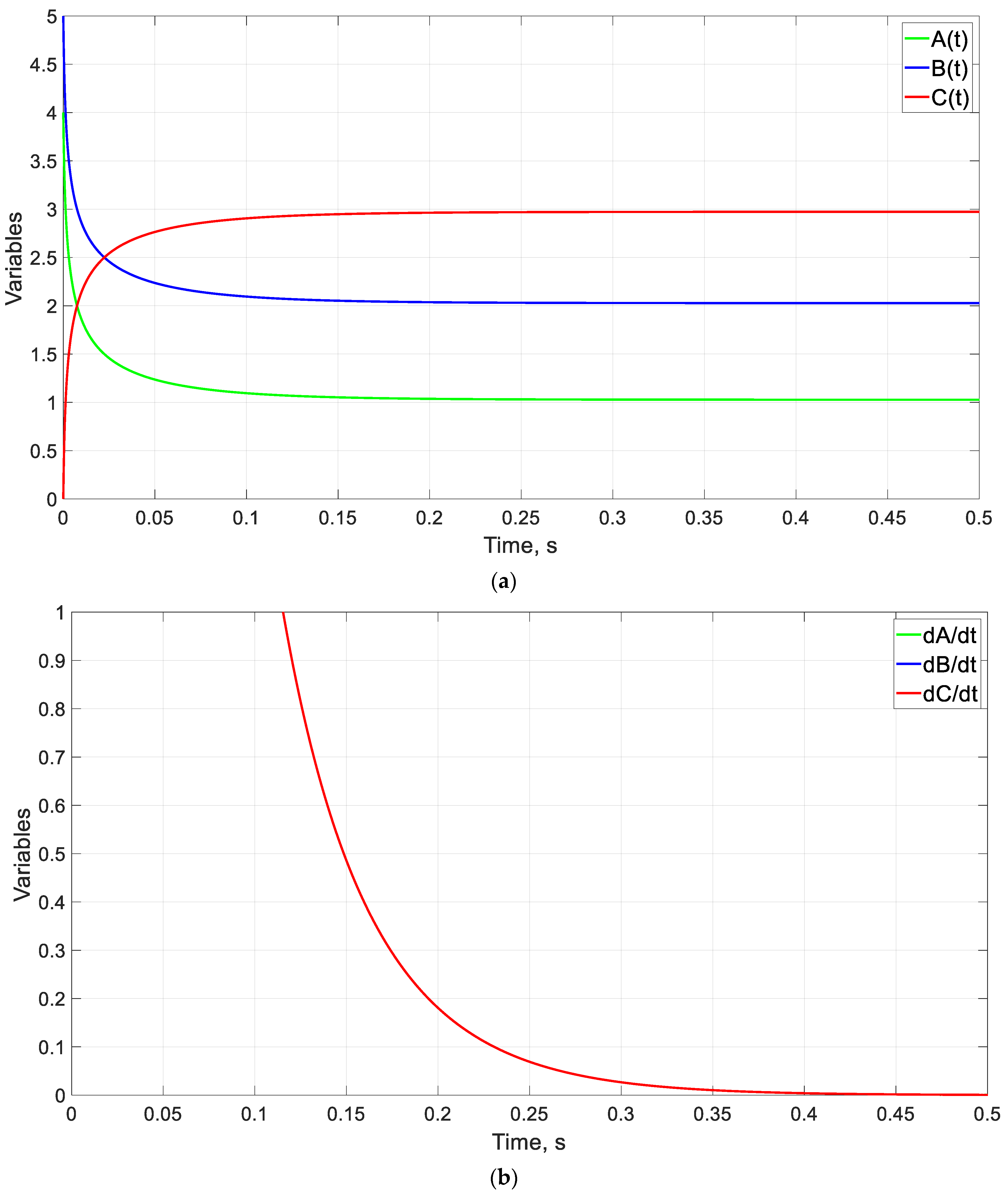
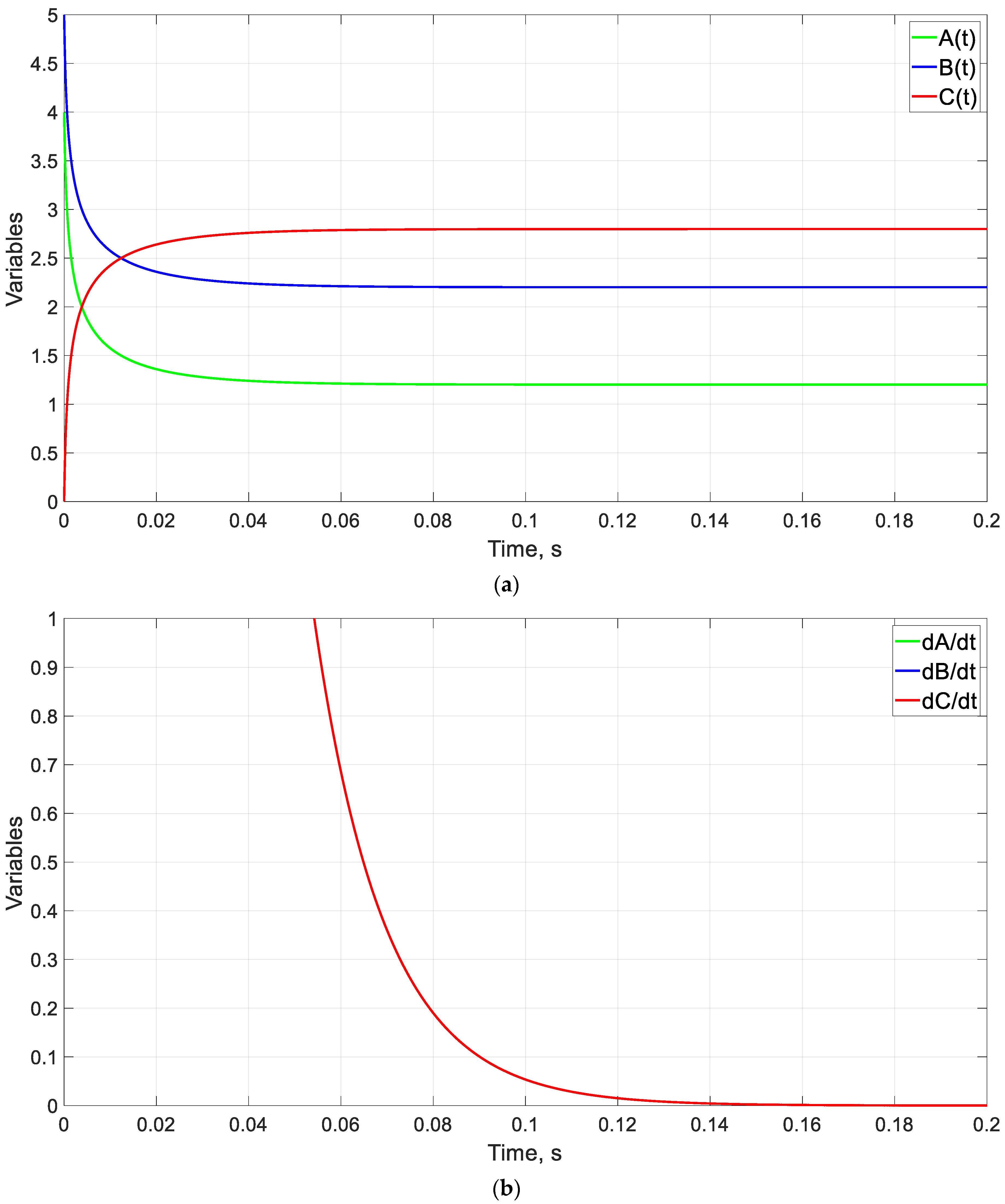
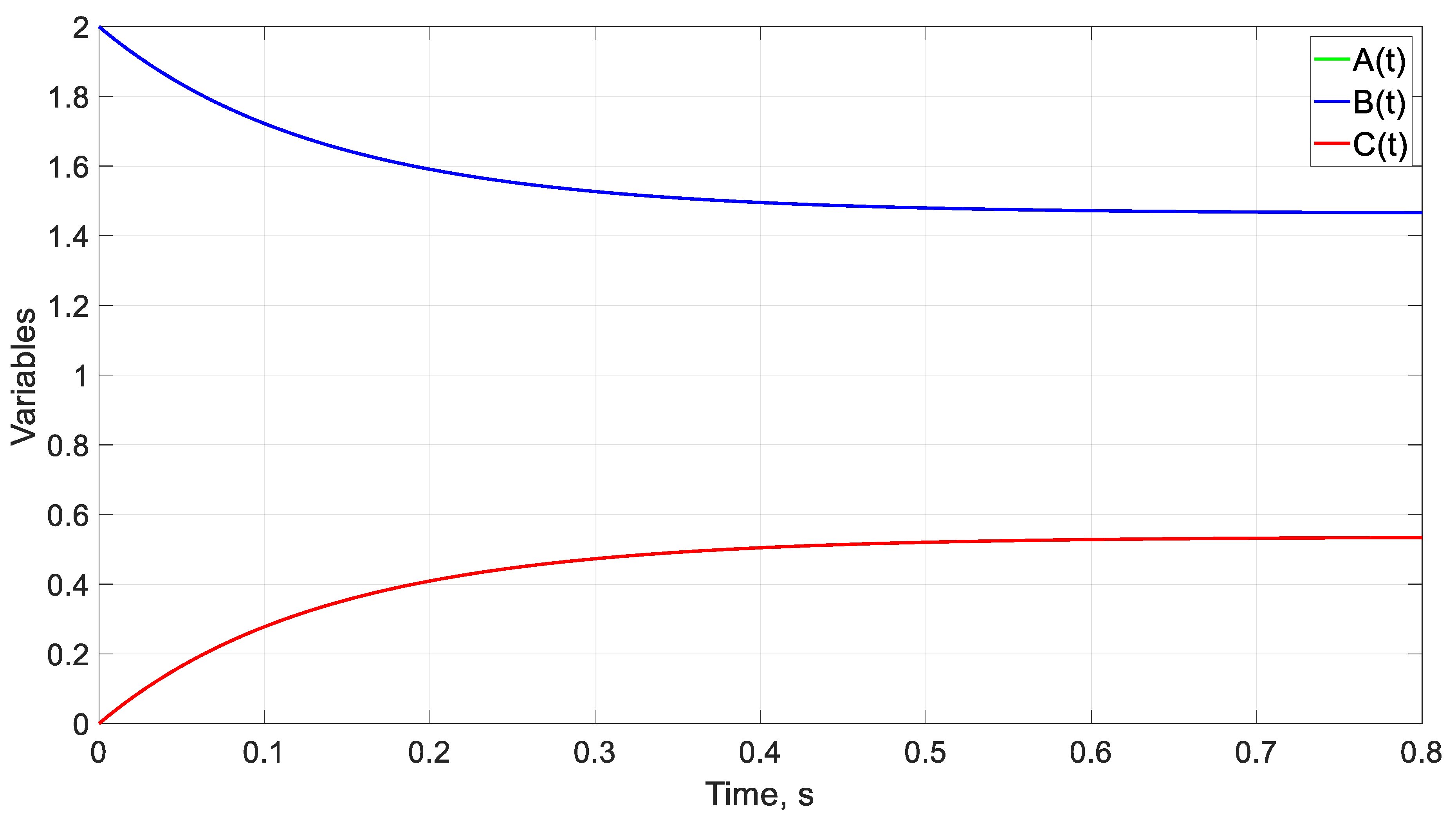
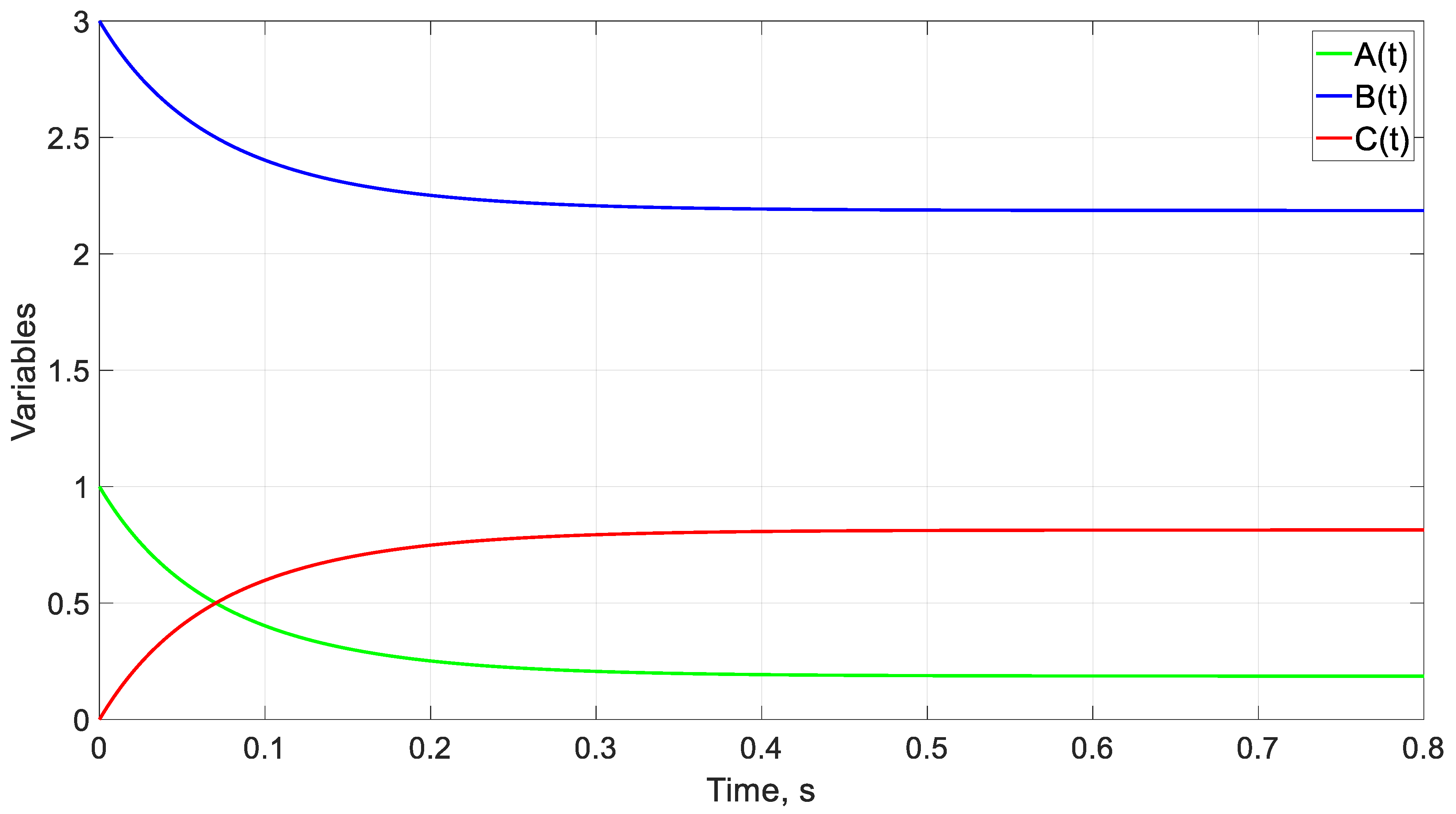
First, we compare the results between cases 1 and 2, where the value of the characteristic time is approximately reduced by half since k_F is double and the functional remains constant, Figure 2 and Figure 3. Similarly, the same occurs in the comparison between cases 1 and 3, where the characteristic time is doubled as k_F is halved, Figure 2 and Figure 4. In all the above cases, since the value of the functional remains constant, the stationary values for the three species, A, B, and C, are always the same, changing only the value of the characteristic time. Thus, Figure 5 shows how when varying the functional, changing only the value of r, both the characteristic time and the stationary values of all species are modified. Finally, as previously stated, the velocity with which the species change in absolute value is the same, as can be seen in Figure 2, Figure 3, Figure 4 and Figure 5.

4.2. Example of a Coupled Oscillator

As a second example of a coupled system of differential equations, now with oscillatory tendencies in time, we present a system of coupled oscillators formed by two masses connected by three springs, located on a horizontal surface without friction, attached to opposite walls.

In this system, the mass m₁ is connected to two springs, one with a constant ${\mathrm{k}}_1$ and the other with a constant ${\mathrm{k}}_{\mathrm{c}}$, while the mass m₂ is connected to two springs, one with a constant ${\mathrm{k}}_{\mathrm{c}}$, which extends between ${\mathrm{m}}_1$ and ${\mathrm{m}}_2$, and the other with a constant ${\mathrm{k}}_3$ connecting ${\mathrm{m}}_2$ to a fixed point. The masses have displacements x₁ and x₂, respectively, with respect to their equilibrium positions. The schema of this system is shown in Figure 6.

The figure shows the positions of both masses in their oscillatory motion around the equilibrium position and the forces to which they are subjected. The governing equations of the system, which govern the motion of the masses, are as follows:

$${\mathrm{m}}_1\frac{{\mathrm{d}}^2{\mathrm{x}}_1}{{\mathrm{dt}}^2}=-{\mathrm{k}}_1{\mathrm{x}}_1+{\mathrm{k}}_{\mathrm{c}}{\mathrm{x}}_2-{\mathrm{k}}_{\mathrm{c}}{\mathrm{x}}_1$$

(13)

$${\mathrm{m}}_2\frac{{\mathrm{d}}^2{\mathrm{x}}_2}{{\mathrm{dt}}^2}=-{\mathrm{k}}_2{\mathrm{x}}_2-{\mathrm{k}}_{\mathrm{c}}{\mathrm{x}}_2+{\mathrm{k}}_{\mathrm{c}}{\mathrm{x}}_1$$

(14)

As shown in the figure, in these equations ${\mathrm{x}}_1$ and ${\mathrm{x}}_2$ represent the position of the masses at a given instant, displaced from their equilibrium position, where ${\mathrm{k}}_1$, ${\mathrm{k}}_2$, and ${\mathrm{k}}_{\mathrm{c}}$ are the elastic constants of the springs.

It is important to note that these two equations are coupled, i.e., the position and acceleration of one mass depend on the position and acceleration of the other mass. Therefore, it is necessary to solve these equations simultaneously to obtain the solutions of ${\mathrm{x}}_1\left(\mathrm{t}\right)$ and ${\mathrm{x}}_2\left(\mathrm{t}\right)$.

Since the motion of the masses is related to each other, it is also convenient to use another equation combining (13) and (14):

$${\mathrm{m}}_1\frac{{\mathrm{d}}^2{\mathrm{x}}_1}{{\mathrm{dt}}^2}+{\mathrm{m}}_2\frac{{\mathrm{d}}^2{\mathrm{x}}_2}{{\mathrm{dt}}^2}=-{\mathrm{k}}_1{\mathrm{x}}_1-{\mathrm{k}}_2{\mathrm{x}}_2$$

(15)

This last equation is an equation, in which the constant ${\mathrm{k}}_{\mathrm{c}}$ is not present since it is an equation that represents the motion of the center of mass, so when it comes to its dimensionless form, we will take into account that there is only one characteristic time, ${\mathrm{t}}_0$, and as we will see, a more simplified monomial will emerge from it.

Applying again for this problem the steps described in Section 2 of this work, the first aim is to adopt the appropriate references to obtain the dimensionless equations. This step is one of the most important in the nondimensionalization process, which requires a deep knowledge of the problem addressed since they will be key in the solution reached following this process. For the x-coordinate, the reference will be ${\mathrm{x}}_{\mathrm{M}}={\mathrm{x}}_{1,0}+{\mathrm{x}}_{2,0}$, that is, the sum of the initial displacements of the masses, so that we ensure that the amplitude of the motion of each mass will never be greater than that, confining the dimensionless variables for the length to the interval [0–1] and for the time references, we adopt two characteristic times since the motion of both is coupled, affecting each other’s oscillation. Two references have been chosen as ${\mathrm{t}}_{0,\mathrm{H}}$ and ${\mathrm{t}}_{0,\mathrm{L}}$, which represent the lowest and highest period values, respectively, which will be the ones we seek in our solution. With this choice for the references, the dimensionless variables are as follows:

$${\mathrm{x}}_1{}^{\prime }=\frac{{\mathrm{x}}_1}{{\mathrm{x}}_{\mathrm{M}}}\hspace{1em}{\mathrm{x}}_2{}^{\prime }=\frac{{\mathrm{x}}_2}{{\mathrm{x}}_{\mathrm{M}}}\hspace{1em}{\mathrm{t}}_1{}^{\prime }=\frac{\mathrm{t}}{{\mathrm{t}}_{0,\mathrm{H}}}\hspace{1em}{\mathrm{t}}_2{}^{\prime }=\frac{\mathrm{t}}{{\mathrm{t}}_{0,\mathrm{L}}}$$

(16)

Introducing these variables in (13), (14), and (15), they can be rewritten in their dimensionless form as follows:

$$\left[\frac{{\mathrm{m}}_1{\mathrm{x}}_{\mathrm{M}}}{{\mathrm{t}}_{0,\mathrm{H}}^2}\right]\frac{{\mathrm{d}}^2{\mathrm{x}}_1{}^{\prime }}{{\mathrm{dt}}_1{{}^{\prime }}^2}=-{\mathrm{k}}_1{\mathrm{x}}_{\mathrm{M}}{\mathrm{x}}_1{}^{\prime }+{\mathrm{k}}_{\mathrm{c}}{\mathrm{x}}_{\mathrm{M}}{\mathrm{x}}_2{}^{\prime }-{\mathrm{k}}_{\mathrm{c}}{\mathrm{x}}_{\mathrm{M}}{\mathrm{x}}_1{}^{\prime }$$

(17)

$$\left[\frac{{\mathrm{m}}_2{\mathrm{x}}_{\mathrm{M}}}{{\mathrm{t}}_{0,\mathrm{L}}^2}\right]\frac{{\mathrm{d}}^2{\mathrm{x}}_2{}^{\prime }}{{\mathrm{dt}}_2{{}^{\prime }}^2}=-{\mathrm{k}}_2{\mathrm{x}}_{\mathrm{M}}{\mathrm{x}}_2{}^{\prime }-{\mathrm{k}}_{\mathrm{c}}{\mathrm{x}}_{\mathrm{M}}{\mathrm{x}}_2{}^{\prime }+{\mathrm{k}}_{\mathrm{c}}{\mathrm{x}}_{\mathrm{M}}{\mathrm{x}}_1{}^{\prime }$$

(18)

$$\left[\frac{{\mathrm{m}}_1{\mathrm{x}}_{\mathrm{M}}}{{\mathrm{t}}_0^2}\right]\frac{{\mathrm{d}}^2{\mathrm{x}}_1{}^{\prime }}{{\mathrm{dt}}_1{{}^{\prime }}^2}+\left[\frac{{\mathrm{m}}_2{\mathrm{x}}_{\mathrm{M}}}{{\mathrm{t}}_0^2}\right]\frac{{\mathrm{d}}^2{\mathrm{x}}_2{}^{\prime }}{{\mathrm{dt}}_2{{}^{\prime }}^2}=-{\mathrm{k}}_1{\mathrm{x}}_{\mathrm{M}}{\mathrm{x}}_1{}^{\prime }-{\mathrm{k}}_2{\mathrm{x}}_{\mathrm{M}}{\mathrm{x}}_2{}^{\prime }$$

(19)

Each equation contains the following coefficients, from which we will form the monomials that govern the solution of the problem:

$$\frac{{\mathrm{m}}_1{\mathrm{x}}_{\mathrm{M}}}{{\mathrm{t}}_{0,\mathrm{H}}^2},{ \mathrm{k}}_1{\mathrm{x}}_{\mathrm{M}},{ \mathrm{k}}_{\mathrm{c}}{\mathrm{x}}_{\mathrm{M}}$$

$$\frac{{\mathrm{m}}_2{\mathrm{x}}_{\mathrm{M}}}{{\mathrm{t}}_{0,\mathrm{L}}^2},{ \mathrm{k}}_2{\mathrm{x}}_{\mathrm{M}},{ \mathrm{k}}_{\mathrm{c}}{\mathrm{x}}_{\mathrm{M}}$$

$$\frac{{\mathrm{m}}_1{\mathrm{x}}_{\mathrm{M}}}{{\mathrm{t}}_0^2},\frac{{\mathrm{m}}_2{\mathrm{x}}_{\mathrm{M}}}{{\mathrm{t}}_0^2},{\mathrm{k}}_1{\mathrm{x}}_{\mathrm{M}},{\mathrm{k}}_2{\mathrm{x}}_{\mathrm{M}}$$

From which the following dimensionless monomials can be formed:

$${\mathsf{\pi }}_1=\frac{{\mathrm{k}}_1{\mathrm{t}}_{0,\mathrm{H}}^2}{{\mathrm{m}}_1}\hspace{1em}\hspace{1em}{\mathsf{\pi }}_2=\frac{{\mathrm{k}}_{\mathrm{c}}}{{\mathrm{k}}_1}$$

$${\mathsf{\pi }}_3=\frac{{\mathrm{k}}_2{\mathrm{t}}_{0,\mathrm{L}}^2}{{\mathrm{m}}_2}\hspace{1em}\hspace{1em}{\mathsf{\pi }}_4=\frac{{\mathrm{k}}_{\mathrm{c}}}{{\mathrm{k}}_2}$$

$${\mathsf{\pi }}_5=\frac{{\mathrm{m}}_1}{{\mathrm{m}}_2}\hspace{1em}\hspace{1em}{\mathsf{\pi }}_6=\frac{{\mathrm{k}}_1}{{\mathrm{k}}_2}$$

To obtain ${\mathsf{\pi }}_5$, it has been taken into account that in expression (19) there is only one characteristic time, as mentioned above, leaving this monomial more simplified.

Applying then the π theorem, similar to the previous example, the solution for the characteristic times of each mass can be expressed as follows:

$${\mathrm{t}}_{0,\mathrm{H}}=\sqrt{\frac{{\mathrm{m}}_1}{{\mathrm{k}}_1}}{\mathsf{\Psi }}_1\left(\frac{{\mathrm{k}}_{\mathrm{c}}}{{\mathrm{k}}_1},\frac{{\mathrm{m}}_1}{{\mathrm{m}}_2},\frac{{\mathrm{k}}_1}{{\mathrm{k}}_2}\right)$$

(20)

$${\mathrm{t}}_{0,\mathrm{L}}=\sqrt{\frac{{\mathrm{m}}_2}{{\mathrm{k}}_2}}{\mathsf{\Psi }}_2\left(\frac{{\mathrm{k}}_{\mathrm{c}}}{{\mathrm{k}}_2},\frac{{\mathrm{m}}_1}{{\mathrm{m}}_2},\frac{{\mathrm{k}}_1}{{\mathrm{k}}_2}\right)$$

(21)

In order to verify the solutions obtained for the characteristic times of the two masses through the nondimensionalization process, the parameters of the system, i.e., the elastic constants of the springs, the masses and the initial positions of each of them are varied, intentionally maintaining the ratios between some of them. Therefore, several cases are presented in

Table 2. Cases for the coupled oscillator.

Case	1	2	3	4	5	6	7	8	9	10	11
${\mathrm{k}}_1$	10	10	10	10	10	20	10	20	5	5	5
${\mathrm{k}}_{\mathrm{c}}$	0.5	0.5	0.5	1	4	0.5	0.5	0.5	10	10	10
${\mathrm{k}}_2$	6	6	6	6	6	6	12	12	5	10	5
${\mathrm{m}}_1$	1	4	1	1	1	1	1	1	1	1	1
${\mathrm{m}}_2$	3	3	12	3	3	3	3	3	1	1	0.5
${\mathrm{x}}_{1,0}$	1	1	1	1	1	1	1	1	1	1	1
${\mathrm{x}}_{2,0}$	1	1	1	1	1	0.5	1	0.5	1	1	1
${\mathrm{t}}_{0,\mathrm{L}}$	1.9390	3.8551	1.9391	1.8886	1.6507	1.3885	1.9391	1.3885	1.2555	1.1916	1.0130
${\mathrm{t}}_{0,\mathrm{H}}$	4.2827	4.3122	8.5106	4.1477	3.7230	4.2827	3.0769	3.0769	2.8121	2.3408	2.4637
Ψ1	6.1315	6.0954	6.1320	5.9722	5.2200	6.2096	6.1320	6.2096	2.8074	2.6645	2.2651
Ψ2	1.2363	1.2448	2.4694	1.6933	3.0398	1.2363	0.6281	0.6281	3.9770	2.3408	3.4841

to check this point. We will see the accuracy of the solutions obtained with the nondimensionalization process from the numerical simulation of the analytical solutions from which we will extract the periods of each movement.

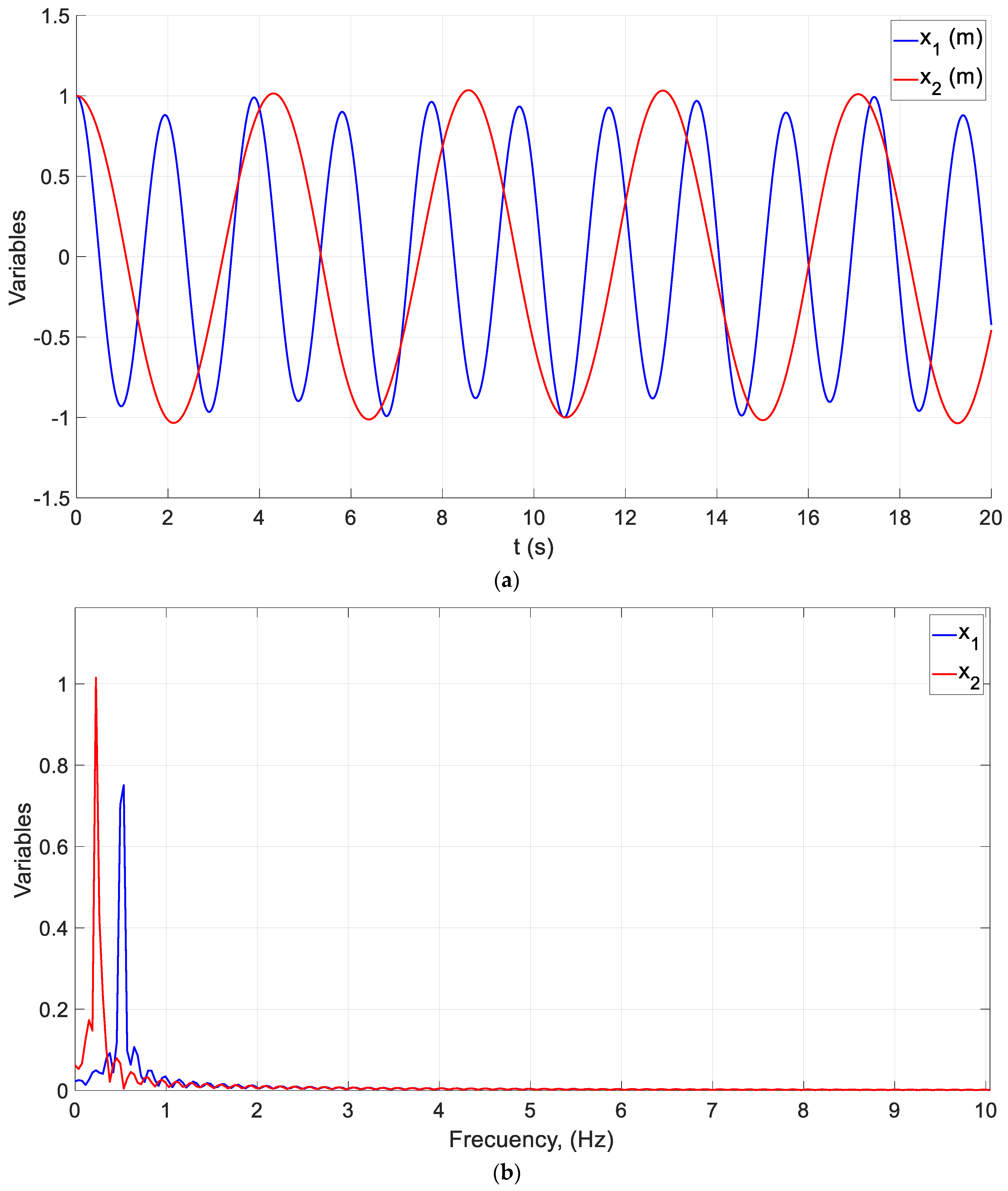
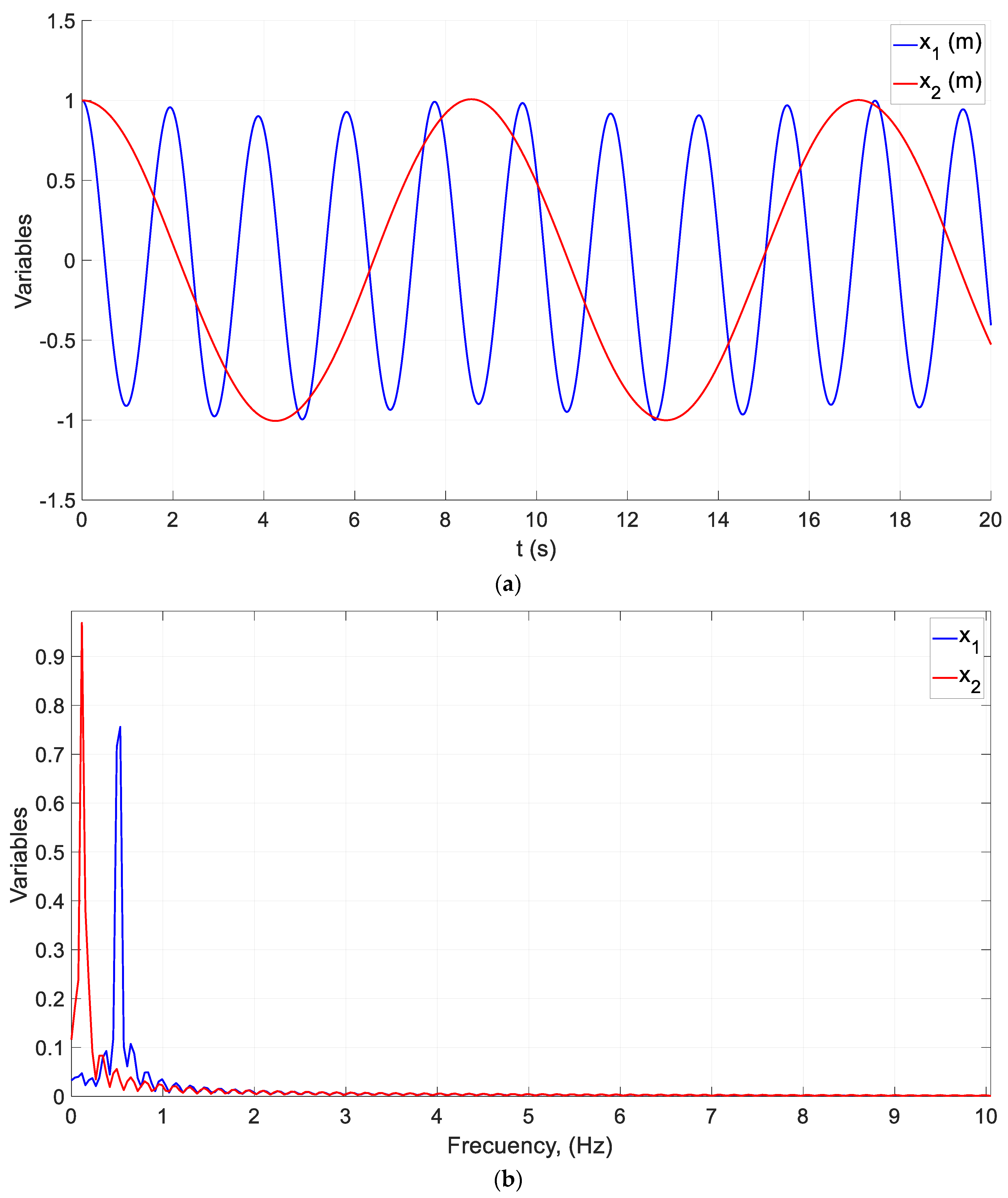
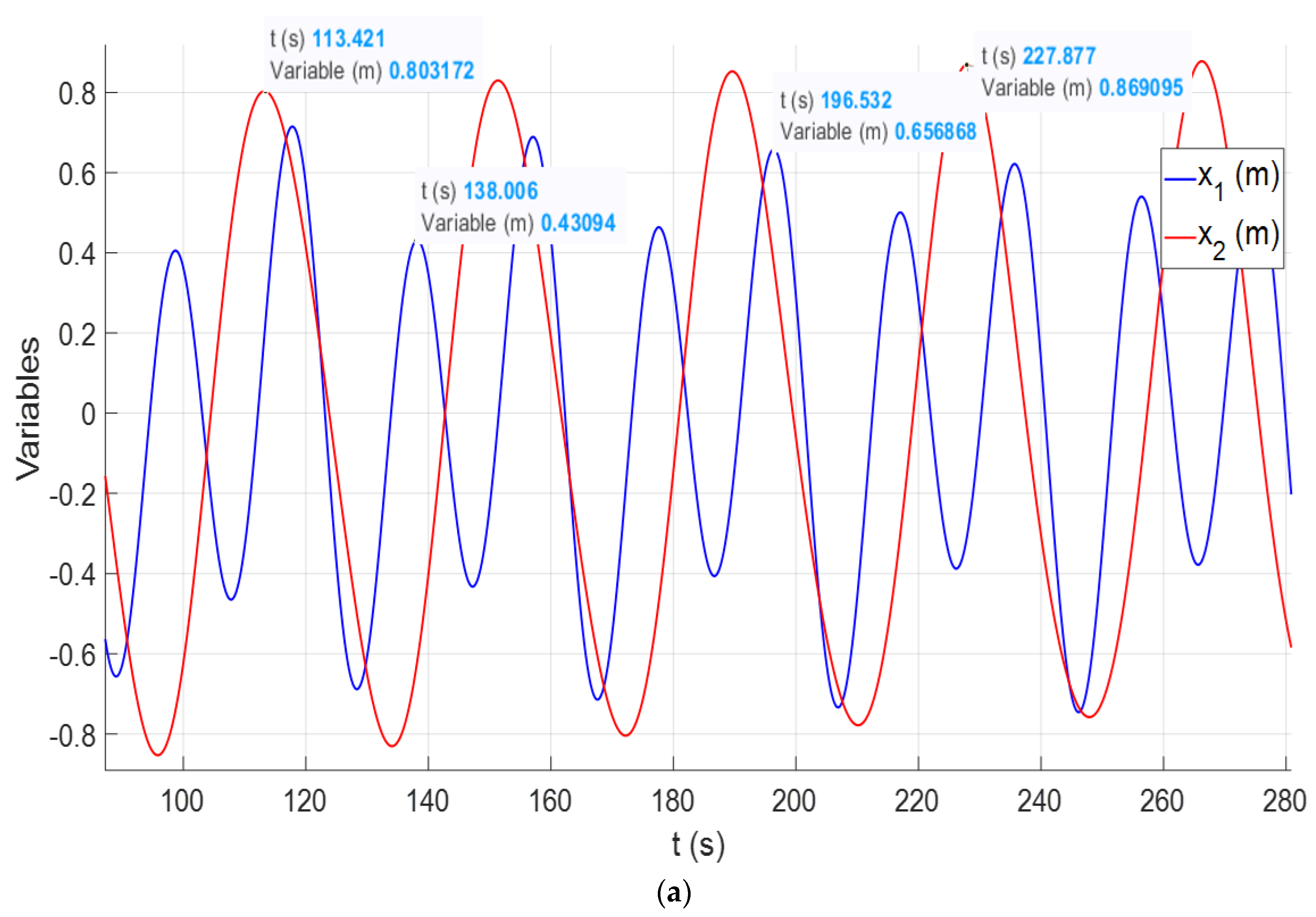
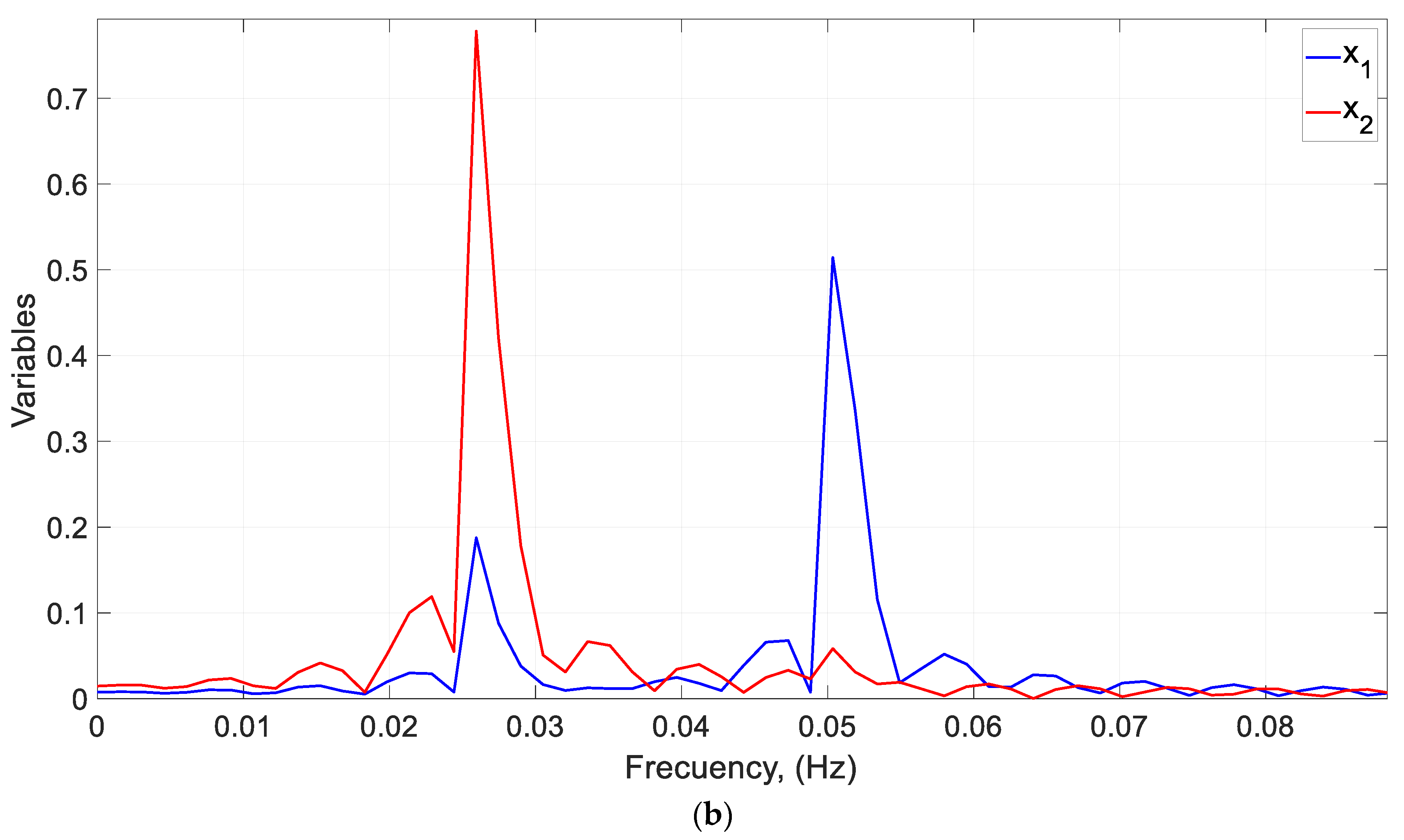
The first thing it can be observed from the data in Table 2 is how in cases 1, 3, and 7, keeping the ratio between m₁ and k₁ constant, the analytical solution extracted from the simulation gives the same period for the three assumptions, t_0,L, and from the solution obtained through the nondimensionalization process it should, also, give the same value for the arbitrary function Ψ₁. It can be seen that this is correct since the values of Ψ₁ are practically the same in these three cases, which have very small variations in the third and fourth decimal places, but there are differences in the Ψ₂ function since the arguments of the function have changed considerably. However, it is observed that between cases 1 and 3, the characteristic time t_0,H has been duplicated, and, therefore, so does the Ψ₂ function, which is consistent with the doubling of π₅, on which this function depends. The simulations of case 1 are shown in Figure 7a; its Fourier frequency spectrum is shown in Figure 7b, from which the periods of both masses have been extracted from their frequency. Furthermore, Figure 8 shows case 3.

The rest of the cases validated show similar behaviors to the one mentioned in the previous paragraph; in fact, it can be observed how the value of the Ψ₁ function has a value close to 6 in all cases from 1 to 8, where either the same ratio between m₁ and k₁ has been maintained or the period extracted in the Fourier frequency simulation for m₁ has varied in the same proportion, thus demonstrating the accuracy of the solution obtained by the nondimensionalization process.

Finally, in cases 9, 10, and 11, ratios different from the previous cases have been used, so the values of the arbitrary functions are different, although maintaining the same trend in the accuracy of the solutions reached by the methodology presented in this work.

5. Functionals Adjustment: Universal Curves

The information provided by the methodology shown in Section 2 and applied in Section 4 is very important since the grouping of the variables in the monomials provides us with information on the weight that a variable has on the problem posed. However, the purpose of this methodology is to obtain universal solutions to different science and engineering problems. To do this, the following the steps shown in Section 2, two more should be added:

v)

Obtaining the functionals

Applying the π-theorem in the previous step, we have obtained expressions of the form π₁ = Ψ (π₂, π₃, …., π_n). Thus, to obtain the functional, an adjustment is made representing two monomials, for example, π₁ and π₂, and keeping the rest constant, obtaining an equation for each constant value that is assigned to the rest of the monomials. For example, for the equation π₁ = Ψ (π₂, π₃), we represent π₁ and π₂ and assign π₃ values 1, 2, and so on, so we would have an equation of π₁ and π₂ for each of these values of π₃;

vi)

Obtaining universal curves or universal solutions

To obtain the universal solution or universal curve, the dimensionless variables defined in each problem are represented, which, given their own definition, will be found in the interval of values [0–1].

5.1. Example of a Continuous Flow Chemical Reactor

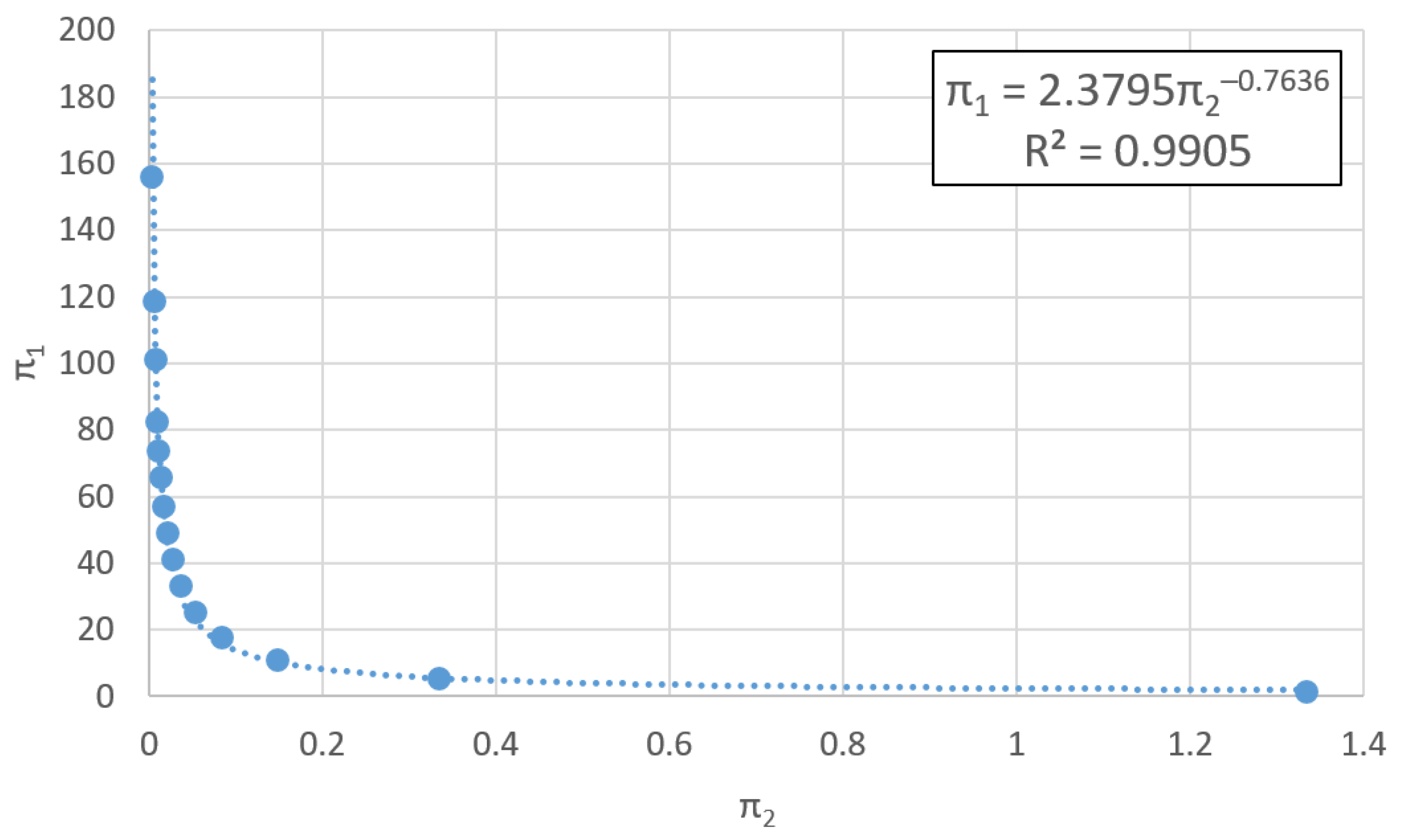
For illustrative purposes, we will obtain both the functionals equations and the universal curves (universal solution) for the problem of continuous flow chemical reactor. After applying the discriminated nondimensionalization methodology to the problem, Equations (10)–(12) arise. Since the three expressions provide the characteristic time, we select one of them that does not contain any unknown to obtain the value of the functional, in this case, Equation (10), ${\mathrm{t}}_{\mathrm{o}} \sim \left[\frac{1}{{\mathrm{k}}_{\mathrm{F}}{\mathrm{A}}_{\mathrm{o}}^{\mathsf{\alpha }-1}{\mathrm{B}}_{\mathrm{o}}^{\mathsf{\beta }}}\right]{\mathsf{\Psi }}_{\mathrm{a}}\left(\frac{\mathrm{r}}{{\mathrm{k}}_{\mathrm{F}}{\mathrm{A}}_{\mathrm{o}}^{\mathsf{\alpha }-1}{\mathrm{B}}_{\mathrm{o}}^{\mathsf{\beta }}}\right)$ or ${\mathsf{\pi }}_1={\mathsf{\Psi }}_{\mathrm{a}}\left({\mathsf{\pi }}_2\right)$ with ${\mathsf{\pi }}_{1,\mathrm{A}}={\mathsf{\pi }}_1=\left[{\mathrm{t}}_{\mathrm{o}}{\mathrm{k}}_{\mathrm{F}}{\mathrm{A}}_{\mathrm{o}}^{\mathsf{\alpha }-1}{\mathrm{B}}_{\mathrm{o}}^{\mathsf{\beta }}\right]$ and ${\mathsf{\pi }}_{2,\mathrm{A}}={\mathsf{\pi }}_2=\left[\frac{\mathrm{r}}{{\mathrm{k}}_{\mathrm{F}}{\mathrm{A}}_{\mathrm{o}}^{\mathsf{\alpha }-1}{\mathrm{B}}_{\mathrm{o}}^{\mathsf{\beta }}}\right]$, was obtained as a solution.

By applying step v), the value of the ${\mathsf{\Psi }}_{\mathrm{a}}$ functional can be obtained, that is if ${\mathsf{\pi }}_1$ is represented against ${\mathsf{\pi }}_2$ (Figure 9) Equation (22) is obtained by regression adjustment, which can be rewritten to obtain the unknown ${\mathrm{t}}_{\mathrm{o}}$, Equation (23). The value obtained for R², the coefficient of determination, indicates that the fit is good since the closer it is to unity, the better the adjustment will be. To obtain the values of t_o for the graphical representation (Figure 9), the problem has been simulated using the Network Simulation Method (Section 3).

$${\mathsf{\pi }}_1=2.3795{\mathsf{\pi }}_2{}^{-0.7636}\hspace{1em}\hspace{1em}{\mathrm{R}}^2=0.9905$$

(22)

$${\mathrm{t}}_{\mathrm{o}}=\frac{1}{{\mathrm{k}}_{\mathrm{F}}{\mathrm{A}}_{\mathrm{o}}^{\mathsf{\alpha }-1}{\mathrm{B}}_{\mathrm{o}}^{\mathsf{\beta }}}{\left(\frac{\mathrm{r}}{{\mathrm{k}}_{\mathrm{F}}{\mathrm{A}}_{\mathrm{o}}^{\mathsf{\alpha }-1}{\mathrm{B}}_{\mathrm{o}}^{\mathsf{\beta }}}\right)}^{-0.7636}$$

(23)

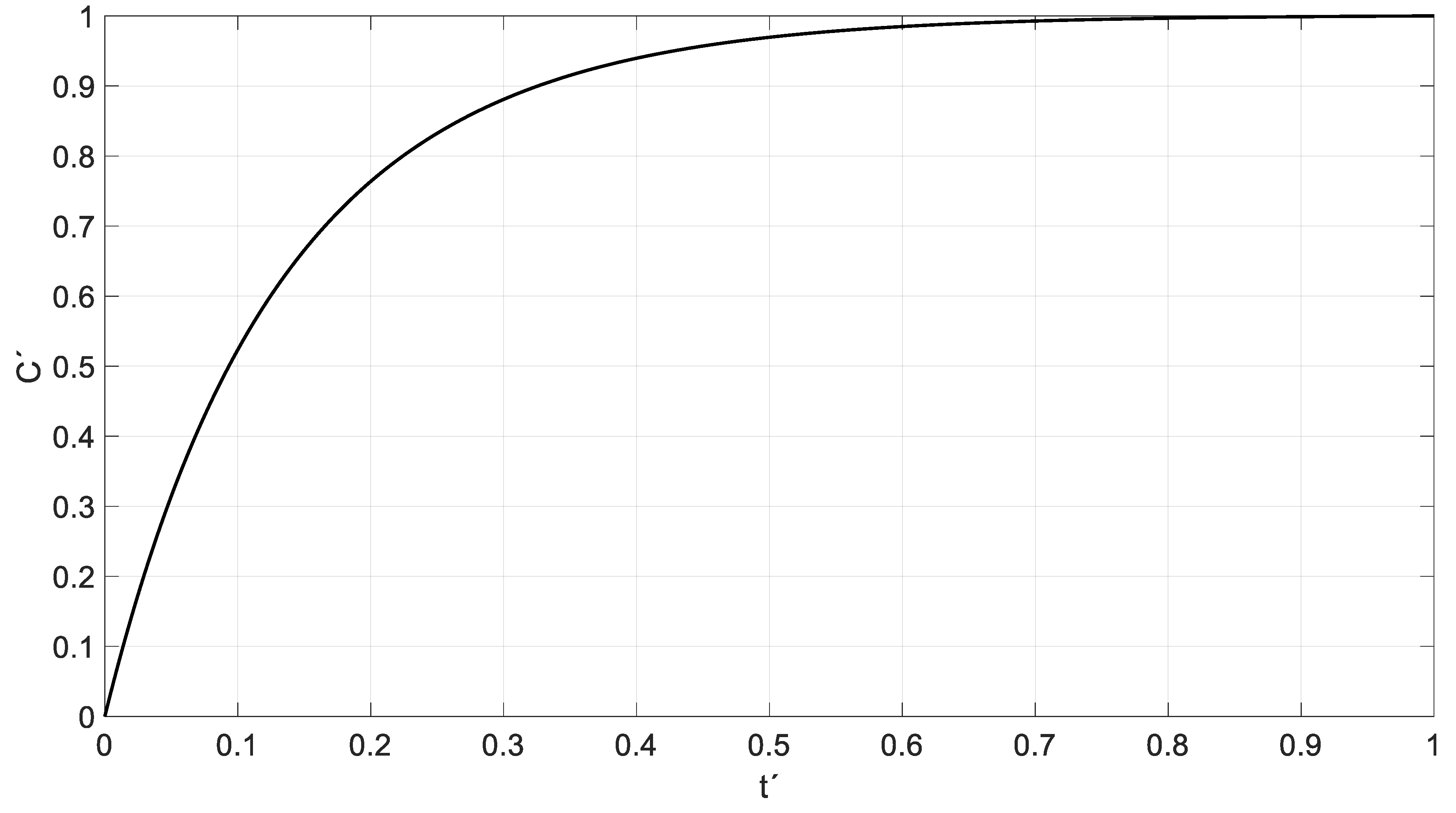
Then, step vi) is applied by simulating the problem for the dimensionless variables, in this case, ${\mathrm{C}}^{\prime }$ and ${\mathrm{t}}^{\prime }$, with ${\mathrm{C}}^{\prime }=\frac{\mathrm{C}}{{\mathrm{C}}_{\mathrm{F}}}$ and ${\mathrm{t}}^{\prime }=\frac{\mathrm{t}}{{\mathrm{t}}_{\mathrm{o}}}$, thus obtaining the universal curve of the problem, Figure 10. The choice of dimensionless variable ${\mathrm{C}}^{\prime }$ is due to the fact that the decrease in species $\mathrm{A}$ and $\mathrm{B}$ is equal to the increase in variable $\mathrm{C}$ because of the very nature of the problem, Equations (24) and (25). The drawback is that the final value of the species C, ${\mathrm{C}}_{\mathrm{F}}$ is unknown. To obtain it, we take the zero reaction rate, $\frac{\mathrm{dA}}{\mathrm{dt}}=\frac{\mathrm{dB}}{\mathrm{dt}}=\frac{\mathrm{dC}}{\mathrm{dt}}=0$, that is, when the steady state is reached, Equations (26)–(28), and the system is solved by Ruffini’s rule or another equation system resolution technique.

$$\mathrm{A}={\mathrm{A}}_{\mathrm{o}}-\Delta \mathrm{A}={\mathrm{A}}_{\mathrm{o}}-\mathrm{C}$$

(24)

$$\mathrm{B}={\mathrm{B}}_{\mathrm{o}}-\Delta \mathrm{B}={\mathrm{B}}_{\mathrm{o}}-\mathrm{C}$$

(25)

$$0=-{\mathrm{k}}_{\mathrm{F}}{\mathrm{A}}_{\mathrm{F}}^{\mathsf{\alpha }}{\mathrm{B}}_{\mathrm{F}}^{\mathsf{\beta }}-\mathrm{r}\left({\mathrm{A}}_{\mathrm{F}}-{\mathrm{A}}_{\mathrm{o}}\right)$$

(26)

$$0=-{\mathrm{k}}_{\mathrm{F}}{\mathrm{A}}_{\mathrm{F}}^{\mathsf{\alpha }}{\mathrm{B}}_{\mathrm{F}}^{\mathsf{\beta }}-\mathrm{r}\left({\mathrm{B}}_{\mathrm{F}}-{\mathrm{B}}_{\mathrm{o}}\right)$$

(27)

$$0={\mathrm{k}}_{\mathrm{F}}{\mathrm{A}}_{\mathrm{F}}^{\mathsf{\alpha }}{\mathrm{B}}_{\mathrm{F}}^{\mathsf{\beta }}-{\mathrm{rC}}_{\mathrm{F}}$$

(28)

A_F, B_F, and C_F are the final or stationary values of each species. To facilitate the resolution of the problem, $\mathsf{\alpha }=\mathsf{\beta }=1$ is going to be taken since it is common for stoichiometric coefficients and exponents to coincide. In this way, the system of Equations (26)–(28) can be rewritten in explicit form, Equations (29)–(31).

$${\mathrm{A}}_{\mathrm{F}}=\frac{-\left({\mathrm{k}}_{\mathrm{F}}{\mathrm{B}}_{\mathrm{o}}-{\mathrm{k}}_{\mathrm{F}}{\mathrm{A}}_{\mathrm{o}}+\mathrm{r}\right)\pm \sqrt{{\left({\mathrm{k}}_{\mathrm{F}}{\mathrm{B}}_{\mathrm{o}}-{\mathrm{k}}_{\mathrm{F}}{\mathrm{A}}_{\mathrm{o}}+\mathrm{r}\right)}^2-\left(4{\mathrm{k}}_{\mathrm{F}}\left(-{\mathrm{rA}}_{\mathrm{o}}\right)\right)}}{2{\mathrm{k}}_{\mathrm{F}}}$$

(29)

$${\mathrm{B}}_{\mathrm{F}}=\frac{\mathrm{r}\left({\mathrm{A}}_{\mathrm{o}}-{\mathrm{A}}_{\mathrm{F}}\right)}{{\mathrm{k}}_{\mathrm{F}}{\mathrm{A}}_{\mathrm{F}}}$$

(30)

$${\mathrm{C}}_{\mathrm{F}}=\frac{{\mathrm{k}}_{\mathrm{F}}{\mathrm{A}}_{\mathrm{F}}{\mathrm{B}}_{\mathrm{F}}}{\mathrm{r}}$$

(31)

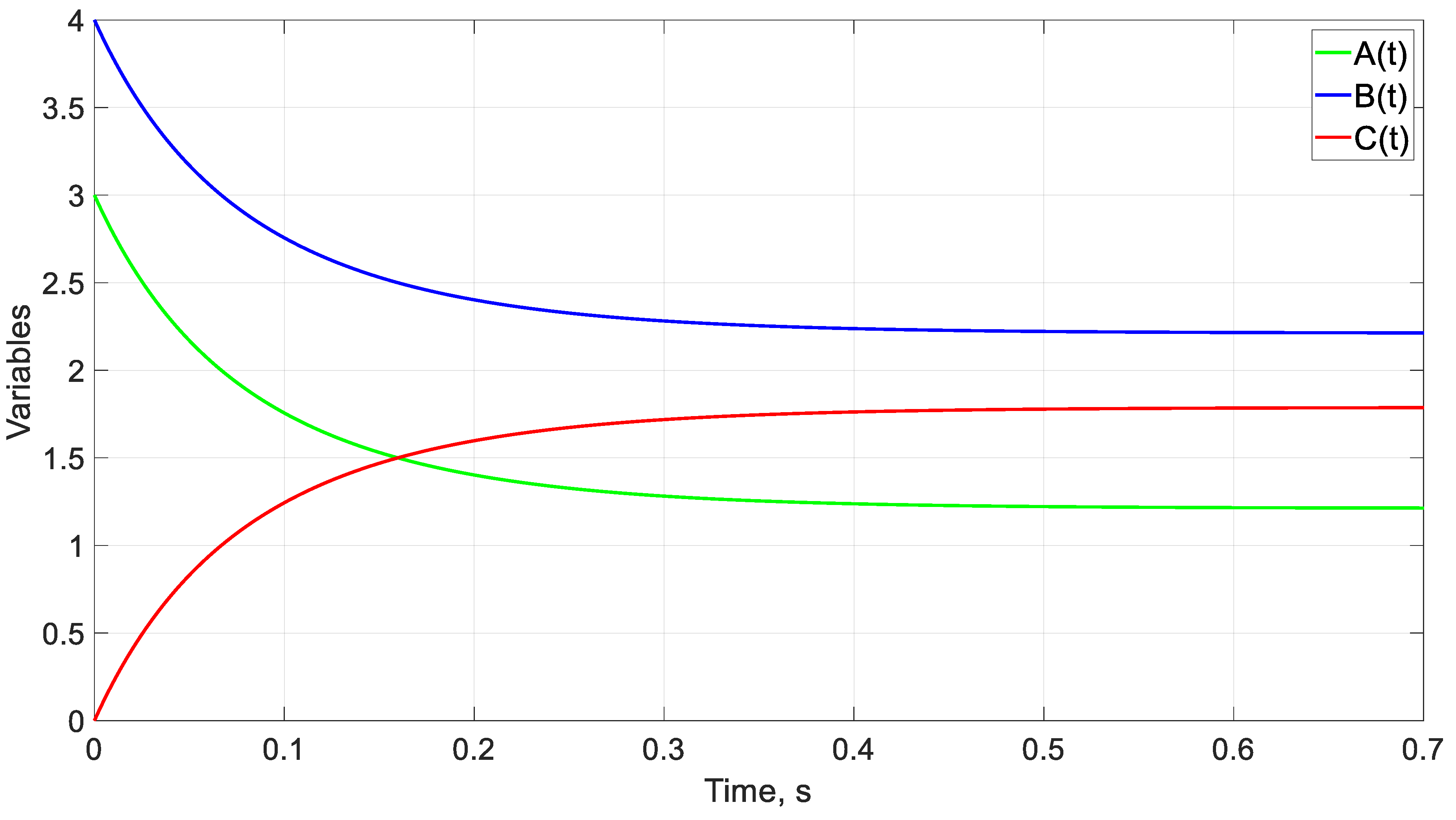
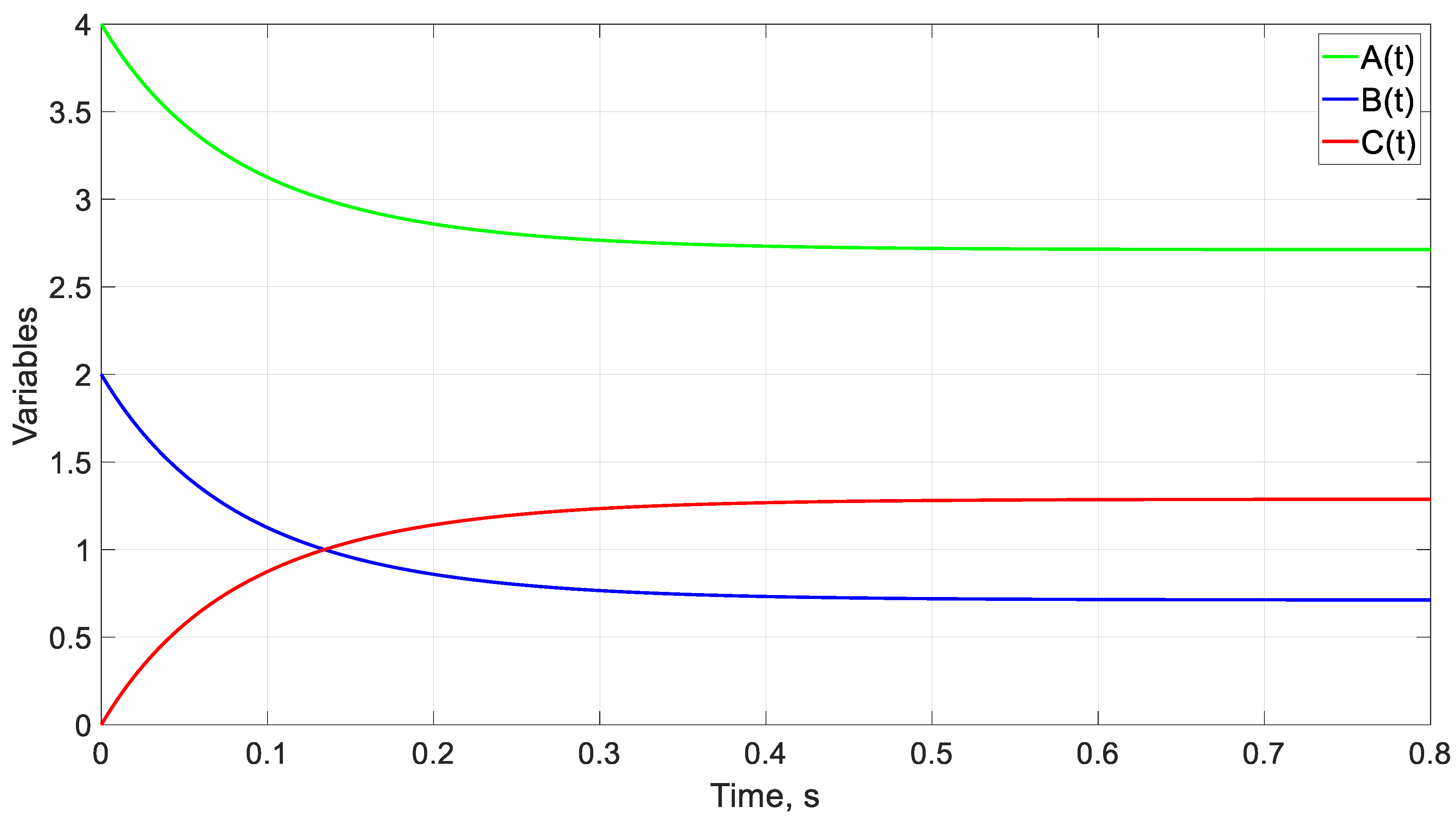
In order to validate the previous expressions, a series of examples will be solved to compare the species values, $\mathrm{A}$, $\mathrm{B},$ and C, obtained by simulation and those obtained via the universal curve. As previously indicated, the method to simulate the problem is the Network Simulation Method. To obtain the value of species C using the universal curve, t_o must first be calculated with Equation (23), and later, A_F, B_F, and C_F with expressions (29)–(31). Then, ${\mathrm{t}}^{\prime }$ is calculated (${\mathrm{t}}^{\prime }=\frac{\mathrm{t}}{{\mathrm{t}}_{\mathrm{o}}}$). Later, ${\mathrm{C}}^{\prime }$ is calculated with the universal curve, Figure 7. Finally, species $\mathrm{C}$ is obtained with C = C′C_F, and species $\mathrm{A}$ and $\mathrm{B}$ with Equations (24) and (25). In order to compare the simulated values with those obtained via the universal curve, different times t will be used.

Table 3. Comparison between simulated values and those calculated via the universal curve.

						Simulated			Unviversal Curves
Case	${\mathbf{A}}_{\mathbf{o}}$	${\mathbf{B}}_{\mathbf{o}}$	KF	r	t (s)	A	$\mathbf{B}$	$\mathbf{C}$	$\mathbf{A}$	$\mathbf{B}$	$\mathbf{C}$	to (s)
1	3	4	2	3	0.1	1.75	2.75	1.24	1.77	2.77	1.23	0.63
2	4	2	2	3	0.2	2.85	0.86	1.14	2.90	0.90	1.10	0.74
3	2	2	1	4	0.3	1.53	1.53	0.47	1.49	1.49	0.51	0.70
4	1	3	4	2	0.4	0.19	2.19	0.81	0.21	2.21	0.79	0.78

shows the comparison between simulated and calculated values, Figure 11, Figure 12, Figure 13 and Figure 14. It should be noted that the differences are due to the number of decimals used in the different expressions and the fitting of the equations.

5.2. Example of a Coupled Oscillator

In this subsection, we will obtain the universal curves (universal solutions) for the coupled oscillator problem. After applying the discriminated nondimensionalization methodology to the problem, Equations (17)–(19) emerged. Since each of the two characteristic times is given by two expressions, any of the expressions (17) or (19) (for i = 1) is valid to obtain t_0,L. Similarly, any of the expressions (18) or (19) (for i = 2) is valid to obtain t_0,H.

In order to simplify the use of universal curves as much as possible, we are going to renumber the dimensionless groups that governed Equations (17)–(19).

$${\mathsf{\pi }}_2=\frac{{\mathrm{k}}_1}{{\mathrm{k}}_{\mathrm{c}}}\hspace{1em}{\mathsf{\pi }}_3=\frac{{\mathrm{k}}_1}{{\mathrm{k}}_2}\hspace{1em}{\mathsf{\pi }}_4=\frac{{\mathrm{m}}_1}{{\mathrm{m}}_2}$$

In this way, from Equations (17) and (19) (for i = 1), two expressions (alternative one to the other) are deduced for the low characteristic period, (${\mathrm{t}}_{0,\mathrm{L}}$):

$${\mathrm{t}}_{0,\mathrm{L}}=\sqrt{\frac{{\mathrm{m}}_1}{{\mathrm{k}}_1}}{\mathsf{\Psi }}_{1,1}\left(\frac{{\mathrm{k}}_1}{{\mathrm{k}}_{\mathrm{c}}},\frac{{\mathrm{k}}_1}{{\mathrm{k}}_2},\frac{{\mathrm{m}}_1}{{\mathrm{m}}_2}\right)$$

(32)

$${\mathrm{t}}_{0,\mathrm{L}}=\sqrt{\frac{{\mathrm{m}}_2}{{\mathrm{k}}_2}}{\mathsf{\Psi }}_{1,2}\left(\frac{{\mathrm{k}}_1}{{\mathrm{k}}_{\mathrm{c}}},\frac{{\mathrm{k}}_1}{{\mathrm{k}}_2},\frac{{\mathrm{m}}_1}{{\mathrm{m}}_2}\right)$$

(33)

Similarly, for the high characteristic period, (${\mathrm{t}}_{0,\mathrm{H}}$):

$${\mathrm{t}}_{0,\mathrm{H}}=\sqrt{\frac{{\mathrm{m}}_2}{{\mathrm{k}}_2}}{\mathsf{\Psi }}_{2,2}\left(\frac{{\mathrm{k}}_1}{{\mathrm{k}}_{\mathrm{c}}},\frac{{\mathrm{k}}_1}{{\mathrm{k}}_2},\frac{{\mathrm{m}}_1}{{\mathrm{m}}_2}\right)$$

(34)

$${\mathrm{t}}_{0,\mathrm{H}}=\sqrt{\frac{{\mathrm{m}}_1}{{\mathrm{k}}_1}}{\mathsf{\Psi }}_{2,1}\left(\frac{{\mathrm{k}}_1}{{\mathrm{k}}_{\mathrm{c}}},\frac{{\mathrm{k}}_1}{{\mathrm{k}}_2},\frac{{\mathrm{m}}_1}{{\mathrm{m}}_2}\right)$$

(35)

Expressions (32)–(35) explicitly provide the characteristic periods (${\mathrm{t}}_{0,\mathrm{L}}$ and ${\mathrm{t}}_{0,\mathrm{H}}$), but their universal representation has to be calculated in terms of their dimensionless forms, that is:

$${\mathsf{\pi }}_{1,\mathrm{L}}{}_{\mathrm{m}1}={\mathsf{\Psi }}_{1,1}\left({\mathsf{\pi }}_2,{\mathsf{\pi }}_3,{\mathsf{\pi }}_4\right)\hspace{1em}\hspace{1em}\mathrm{with} {\mathsf{\pi }}_{1,\mathrm{L}}{}_{\mathrm{m}1}=\frac{{\mathrm{k}}_1{\mathrm{t}}_{0,\mathrm{L}}{}^2}{{\mathrm{m}}_1}$$

(36)

$${\mathsf{\pi }}_{1,\mathrm{L}}{}_{\mathrm{m}2}={\mathsf{\Psi }}_{1,2}\left({\mathsf{\pi }}_2,{\mathsf{\pi }}_3,{\mathsf{\pi }}_4\right)\hspace{1em}\hspace{1em}\mathrm{with} {\mathsf{\pi }}_{1,\mathrm{L}}{}_{\mathrm{m}2}=\frac{{\mathrm{k}}_2{\mathrm{t}}_{0,\mathrm{L}}{}^2}{{\mathrm{m}}_2}$$

(37)

$${\mathsf{\pi }}_{1,\mathrm{H}}{}_{\mathrm{m}2}={\mathsf{\Psi }}_{2,2}\left({\mathsf{\pi }}_2,{\mathsf{\pi }}_3,{\mathsf{\pi }}_4\right)\hspace{1em}\hspace{1em}\mathrm{with} {\mathsf{\pi }}_{1,\mathrm{H}}{}_{\mathrm{m}2}=\frac{{\mathrm{k}}_2{\mathrm{t}}_{0,\mathrm{H}}{}^2}{{\mathrm{m}}_2}$$

(38)

$${\mathsf{\pi }}_{1,\mathrm{H}}{}_{\mathrm{m}1}={\mathsf{\Psi }}_{2,1}\left({\mathsf{\pi }}_2,{\mathsf{\pi }}_3,{\mathsf{\pi }}_4\right)\hspace{1em}\hspace{1em}\mathrm{with} {\mathsf{\pi }}_{1,\mathrm{H}}{}_{\mathrm{m}1}=\frac{{\mathrm{k}}_1{\mathrm{t}}_{0,\mathrm{H}}{}^2}{{\mathrm{m}}_1}$$

(39)

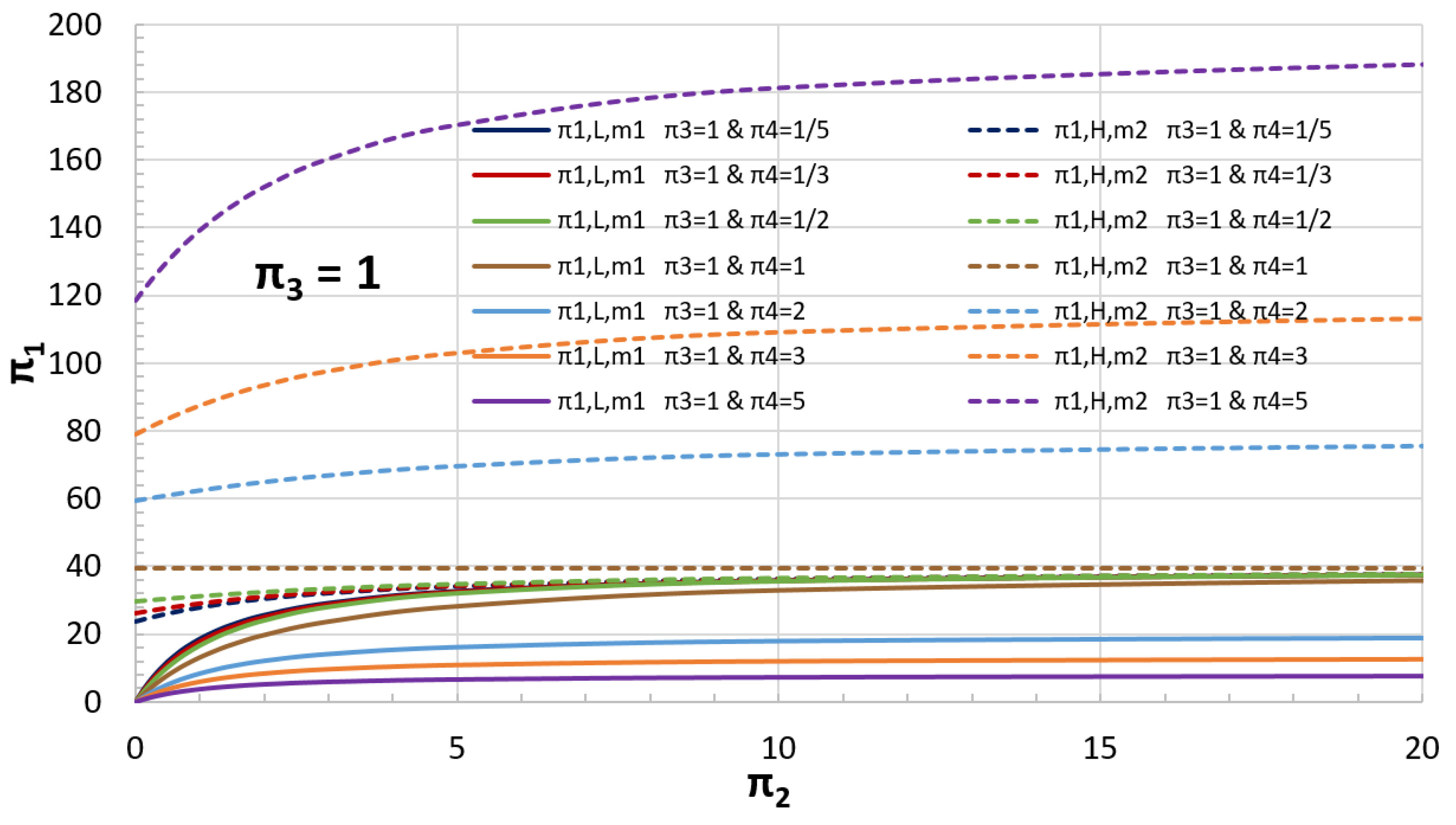
Next, by application of step v) we obtain the functionals ${\mathsf{\Psi }}_{1,1}$, ${\mathsf{\Psi }}_{1,2}$, ${\mathsf{\Psi }}_{2,2}$, and ${\mathsf{\Psi }}_{2,1}$, which allow us to draw the universal curves for the oscillation periods (in their dimensionless expression). The pattern of solutions of the problem depends on three dimensionless groups (${\mathsf{\pi }}_2$, ${\mathsf{\pi }}_3$, and ${\mathsf{\pi }}_4$), but the central spring constant ${\mathrm{k}}_{\mathrm{c}}$ is one of the most influential parameters of the problem. Then, the dimensionless forms of the periods (${\mathsf{\pi }}_1$) will be represented for the entire range of variation of ${\mathsf{\pi }}_2$, while the monomials ${\mathsf{\pi }}_3$ and ${\mathsf{\pi }}_4$ will take specific values. Thus, ${\mathsf{\pi }}_3$ will take the values of 1, 2 and 5. In addition, to use the universal curves below, the criterion that the mass m₁ corresponds to that mass whose spring constant is higher will be taken. That is, it must always be true that ${\mathrm{k}}_1\ge {\mathrm{k}}_2$ (does not apply, then to represent the cases for which ${\mathsf{\pi }}_3$ takes the values of 1/2 and 1/5). As for the monomial related to the ratio of masses, ${\mathsf{\pi }}_4$, it will take the values of 1/5, 1/3, 1/2, 1, 2, 3, and 5. The expressions of the resulting functionals can be obtained by regression adjustment, but since there are 42 curves, their presentation would be cumbersome. However, the charts presented below are easy to use and provide high precision. Figure 15 shows the universal abacus for ${\mathsf{\pi }}_3=\frac{{\mathrm{k}}_1}{{\mathrm{k}}_2}=1$.

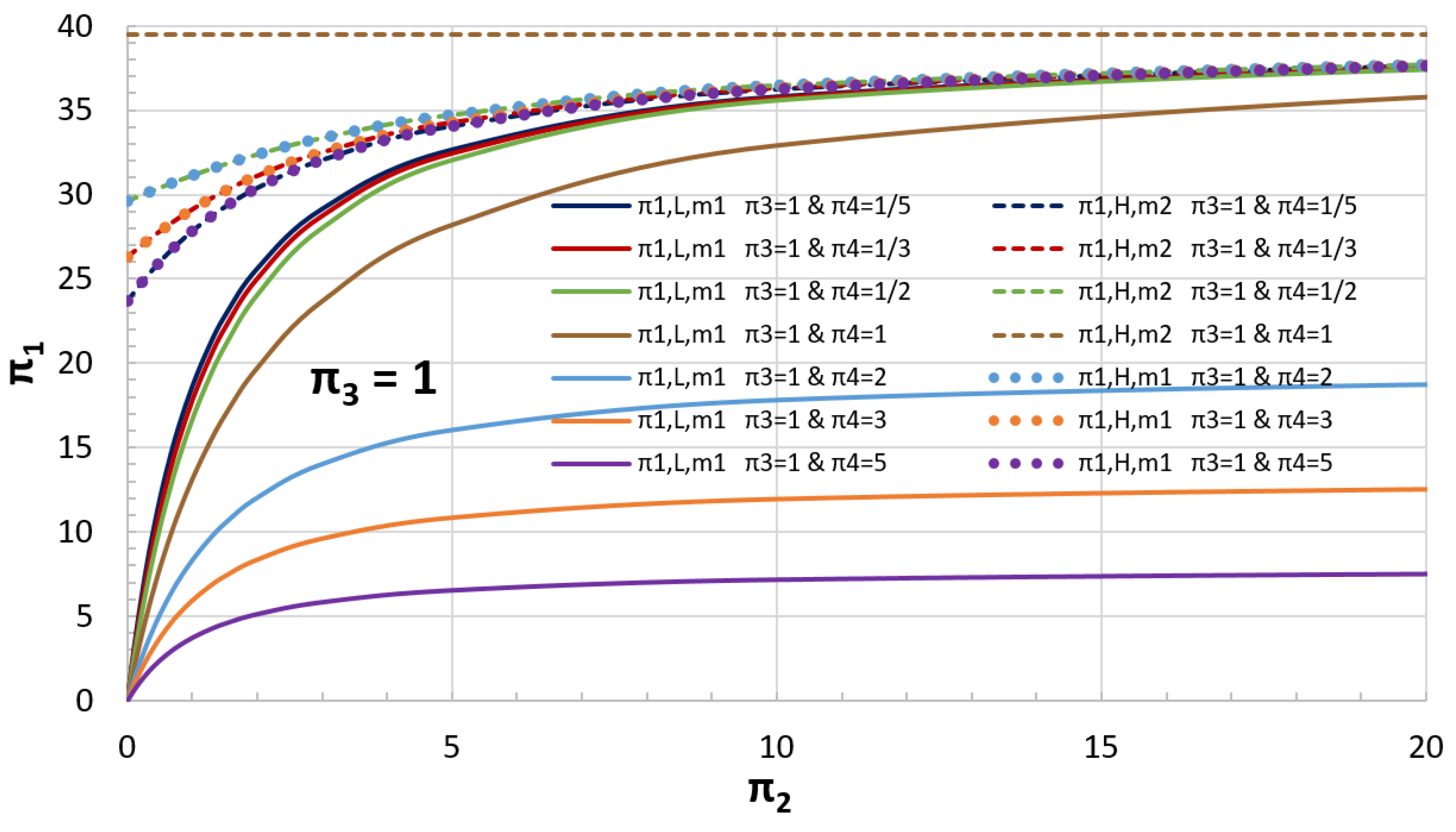
As can be seen, ${\mathrm{t}}_{0,\mathrm{L}}$ appears in its dimensionless form ${\mathsf{\pi }}_{1,\mathrm{L}}{}_{\mathrm{m}1}$ (that is, normalized with mass 1) being bounded in the interval [0,40] for ${\mathsf{\pi }}_1$, while ${\mathrm{t}}_{0,\mathrm{H}}$ is presented in its dimensionless form ${\mathsf{\pi }}_{1,\mathrm{H}}{}_{\mathrm{m}2}$ (normalized with mass 2), remaining bounded in the interval [0,200] for ${\mathsf{\pi }}_1$. This is caused by the curves corresponding with π₄ = $\frac{{\mathrm{m}}_1}{{\mathrm{m}}_2}$ = 2, 3, and 5, which can lead to reading inaccuracies when using the abacus. However, if for these three t_0,H curves we use the (alternative) dimensionless form ${\mathsf{\pi }}_{1,\mathrm{H}}{}_{\mathrm{m}1}$ (normalized with mass 1), the whole graph is bounded in the interval [0,40] for ${\mathsf{\pi }}_1$, Figure 16.

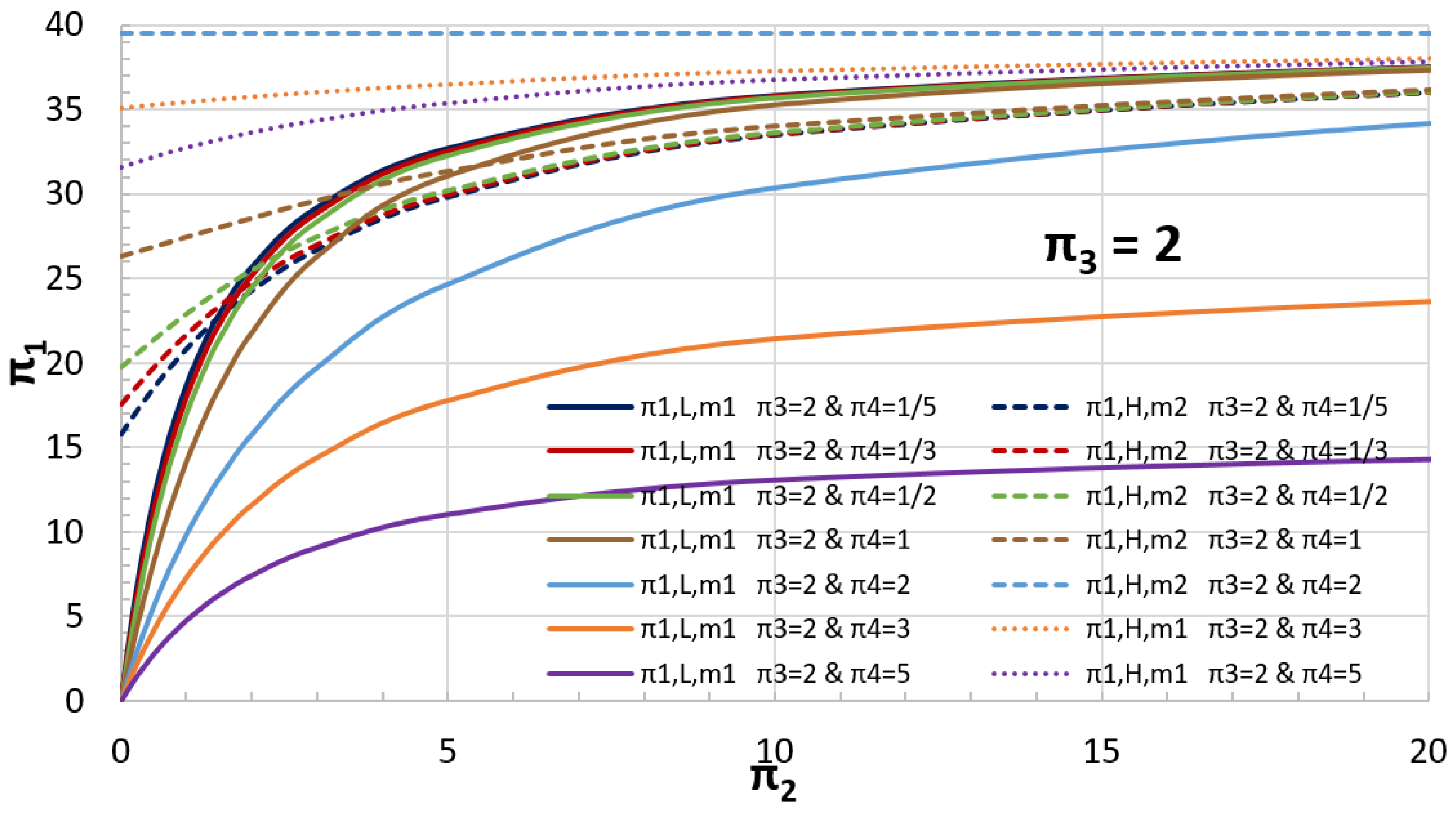
Figure 17 shows the universal abacus for ${\mathsf{\pi }}_3=\frac{{\mathrm{k}}_1}{{\mathrm{k}}_2}=2$. In this chart t_0,L appears in its dimensionless form ${\mathsf{\pi }}_{1,\mathrm{L}}{}_{\mathrm{m}1}$ (normalized with mass 1), while t_0,H is presented in its dimensionless form ${\mathsf{\pi }}_{1,\mathrm{H}}{}_{\mathrm{m}2}$ (normalized with mass 2) for ${\mathsf{\pi }}_4=\frac{{\mathrm{m}}_1}{{\mathrm{m}}_2}=\frac{1}{5},\frac{1}{3},\frac{1}{2}, 1,$ and $2$. On the other hand, for ${\mathsf{\pi }}_4=\frac{{\mathrm{m}}_1}{{\mathrm{m}}_2}=3$ and $5$, the (alternative) dimensionless form ${\mathsf{\pi }}_{1,\mathrm{H}}{}_{\mathrm{m}1}$ (normalized with mass 1) has been used for t_0,H. In this way, the whole graph is bounded in the interval [0,40] for ${\mathsf{\pi }}_1$.

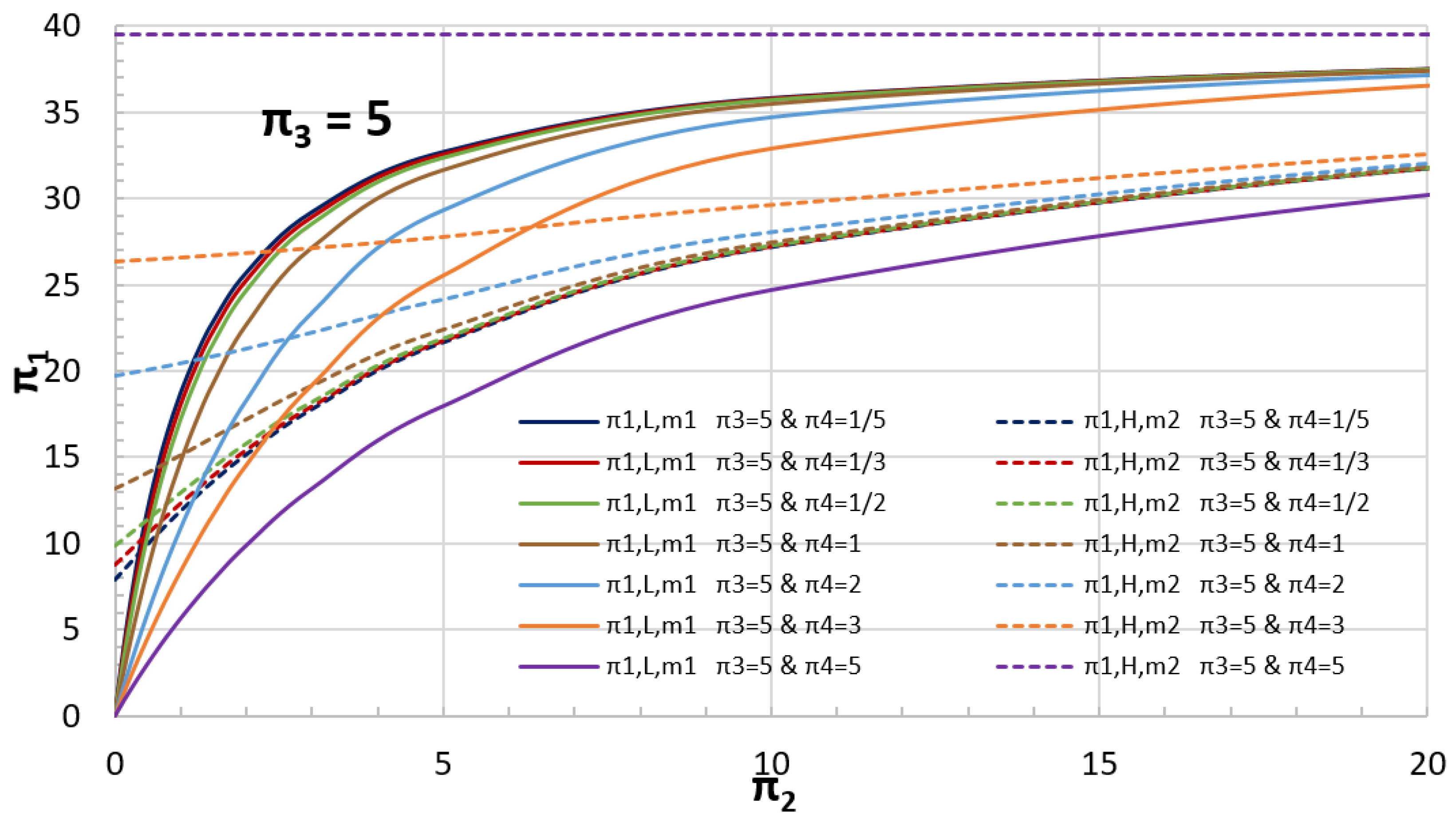
Finally, Figure 18 shows the universal abacus for ${\mathsf{\pi }}_3=\frac{{\mathrm{k}}_1}{{\mathrm{k}}_2}=5$. In this chart t_0,L appears in its dimensionless form ${\mathsf{\pi }}_{1,\mathrm{L}}{}_{\mathrm{m}1}$ (normalized with mass 1), while t_0,H is presented in its dimensionless form ${\mathsf{\pi }}_{1,\mathrm{H}}{}_{\mathrm{m}2}$ (normalized with mass 2), this being enough for the graph bounded in the interval [0,40] for ${\mathsf{\pi }}_1$.

In order to validate the previous charts, a couple of examples will be solved to compare the period values ${\mathrm{t}}_{0,\mathrm{L}}$ and ${\mathrm{t}}_{0,\mathrm{H}}$ obtained by simulation and those obtained with the universal curves. As previously indicated, the method to simulate the problem is the Network Simulation Method. To obtain the values of t_0,L and t_0,H using the universal curves, the values of the monomials ${\mathsf{\pi }}_2$, ${\mathsf{\pi }}_3,$ and ${\mathsf{\pi }}_4$ are calculated from the masses and the spring constants. Once these values are known, the universal curve is chosen according to ${\mathsf{\pi }}_3$ is 1, 2, or 3 (Figure 15, Figure 16, Figure 17 and Figure 18), and, for the values of ${\mathsf{\pi }}_2$ and ${\mathsf{\pi }}_4$, ${\mathsf{\pi }}_{1,\mathrm{L}}{}_{\mathrm{m}1}$ and ${\mathsf{\pi }}_{1,\mathrm{H}}{}_{\mathrm{m}2}$ (or, alternatively, ${\mathsf{\pi }}_{1,\mathrm{H}}{}_{\mathrm{m}1}$) are read in the charts. Once these values are obtained from the expressions (36) and (38), or, alternatively, expression (39), the values of ${\mathrm{t}}_{0,\mathrm{L}}$ and ${\mathrm{t}}_{0,\mathrm{H}}$ are solved.

Table 4. Comparison between simulated values and those calculated with the universal curves.

											Universal Curves				Simulated
Case	k1	kc	k2	m1	m2	x1,0	x2,0	π2	π3	π4	π1,L	π1,H	t0,L	t0,H	t0,L	t0,H
1	12	0.6	2.4	4.5	1.5	1	1/2	20	5	3	36.8	32.6	3.7148	4.5139	3.7141	4.5132
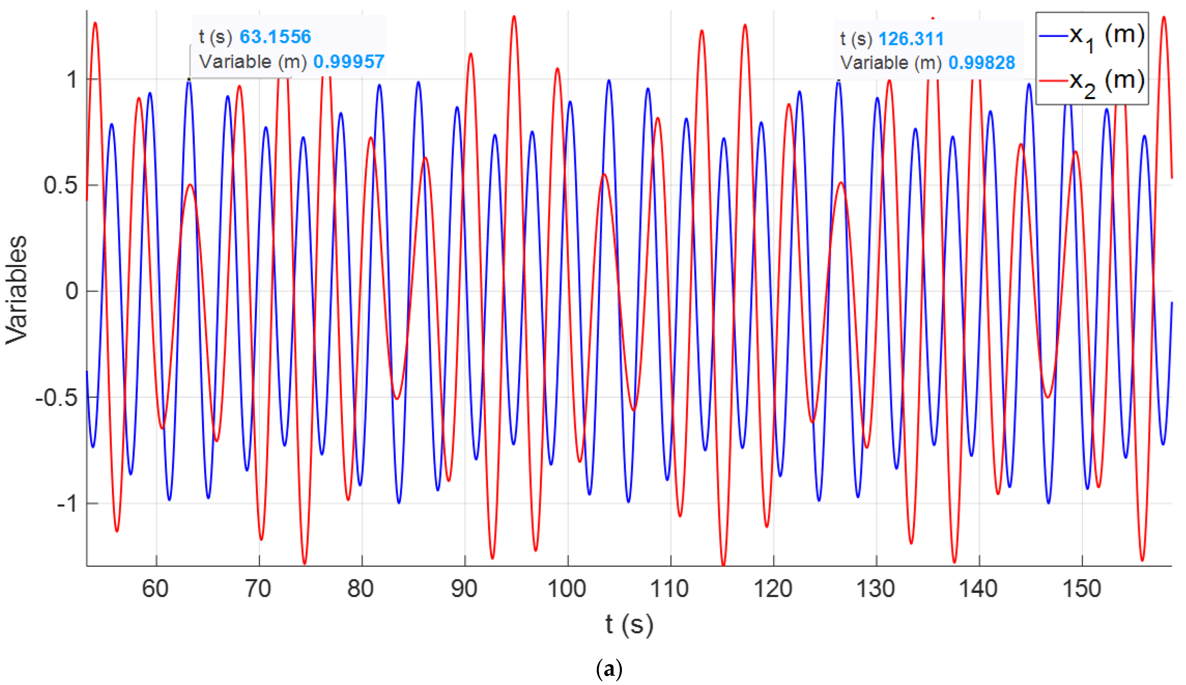
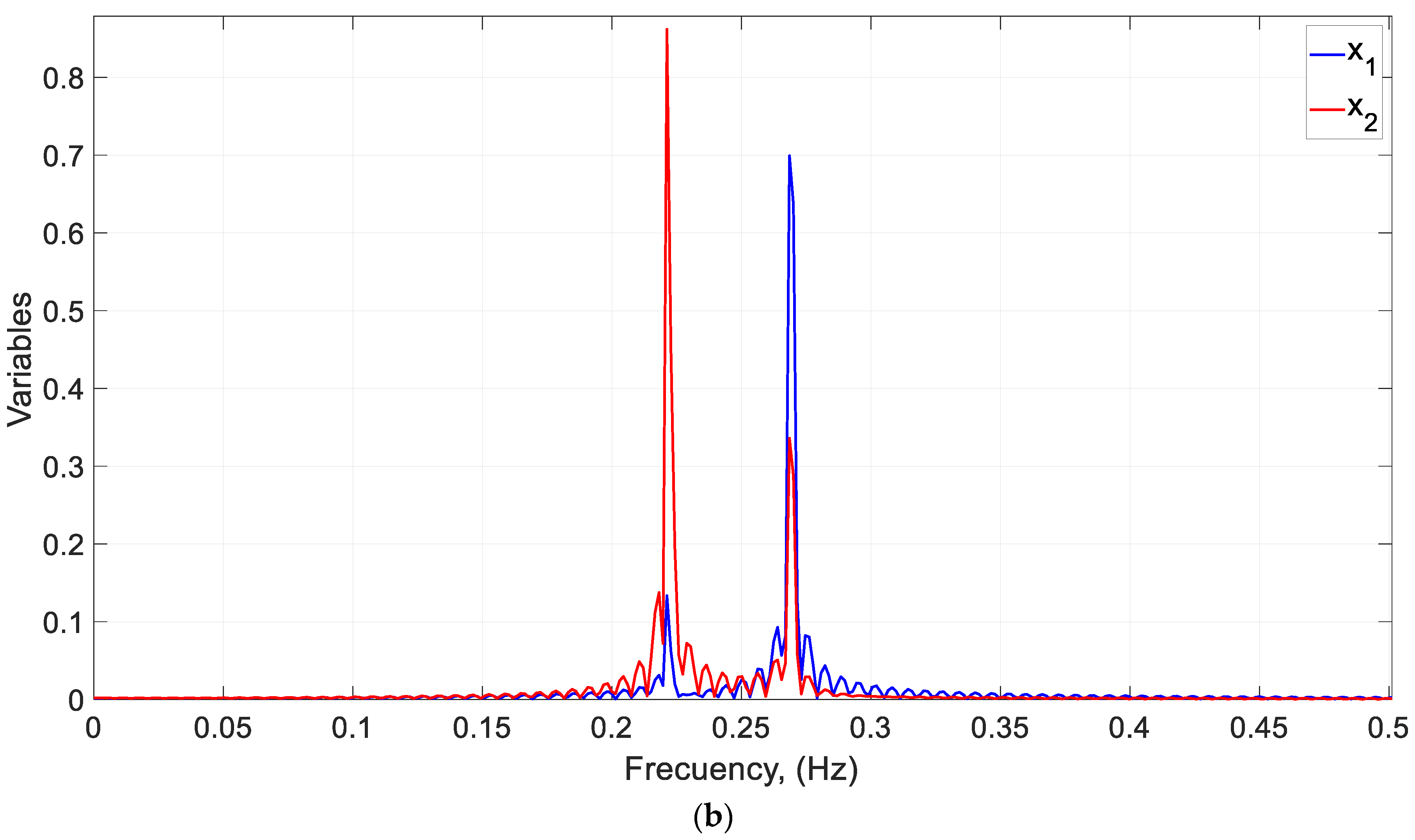
2	1/4	1/20	1/8	3	6	3/4	3/4	5	2	0.5	32.4	30.2	19.7180	38.0736	19.6822	38.0574

shows the comparison between simulated and calculated values of ${\mathrm{t}}_{0,\mathrm{L}}$ and ${\mathrm{t}}_{0,\mathrm{H}}$ for two selected cases. It should be noted that the (slight) differences are due to the precision when reading on the abacuses. Figure 19 and Figure 20 show the oscillatory movement and the characteristic frequencies (inverse of the periods) obtained by spectral analysis for each of the two masses, m₁ and m₂.

6. Conclusions

This paper initially presents the bases to carry out a correct nondimensionalization. The importance of the correct choice of the reference, which implies a deep knowledge of the problem, should be noted since it will allow us to define the dimensionless variables in the numerical interval [0–1], known in this case as normalized variables. The substitution of these variables in the governing equations allows us to obtain dimensionless governing equations, which, through the combination of their coefficients, provide us with the dimensionless monomials that rule the problem. The relationship between the monomials is established through the π-theorem by using functionals. Then, obtaining the expressions of the functionals is performed with regression adjustments using data obtained by numerical simulation. Finally, the abacus of universal curves (solutions) is obtained by simulating the dimensionless variables, which, by their own definition, are in the numerical interval [0–1].

In the first example, the methodology is applied to a coupled system of three chemical species, an illustration of a system of coupled ordinary differential equations. In the cases studied, it is worth noting the relationship of the monomials obtained for each equation, one for each species, with the time until the steady state is reached. Finally, the universal curve of the problem is obtained, and the resolution of several problems is exposed. It should be noted that in this case, the same universal solution includes an unknown that must be previously obtained. The resolution of this unknown implies having a deep knowledge of the problem, a common characteristic when using the methodology proposed in this work for different engineering or physicochemical problems.

Regarding the independent variable, time, a physical inspection of the problem allows us to discern that the system of three chemical species studied only has a temporal reference, the moment in which the steady state is reached, although three expressions are obtained to calculate it. The biggest problem in this case study is the choice of the time value when the mentioned steady state is reached. In previous works, since the evolution curves of the compounds are asymptotic, a certain fraction of their evolution interval has been taken as a reference since some variables tended to disappear or the final value they took was known. In this case, it is not possible since the stationary values that both the reactants and the products will have are unknown. Thus, in this problem, it is taken as a reference the time in which the reaction rate is zero or takes a very small value.

In the second one, a coupled oscillator is studied, where, in the first place, the reference of the amplitude, for correct dimensioning, must be the sum of the initial displacements of both masses since, being coupled, the displacement of one mass can exceed its initial value. On the other hand, the study of the system shows that there are two characteristic periods. Each of them affects the oscillation of each of the masses explicitly or implicitly. Finally, several abacuses of universal curves have been carried out for the universal solution of the characteristic periods.

Finally, the procedure to obtain universal solutions has been shown, highlighting that in complex problems, this methodology could save us long periods of simulations since the same results are obtained with precision.

References

1. Gibbings, J.C. A logic of dimensional analysis. J. Phys. A Math. Gen. 1982, 15, 1991–2002. [Google Scholar] [CrossRef]
2. Gibbings, J.C. On dimensional analysis. J. Phys. A Math. Gen. 1980, 13, 75–89. [Google Scholar] [CrossRef]
3. Gibbings, J.; Hignett, E. Dimensional analysis of electrostatic streaming current. Electrochim. Acta 1966, 11, 815–826. [Google Scholar] [CrossRef]
4. Sonin, A.A. The Physical Basis of Dimensional Analysis; Department of Mechanical Engineering, MIT: Cambridge, MA, USA, 2001. [Google Scholar]
5. Potter, M.C.; Wiggert, D.C.; Ramadan, B.H. Mechanics of Fluids SI Version; Cengage Learning: Boston, MA, USA, 2012. [Google Scholar]
6. Capobianchi, M.; Aziz, A. A scale analysis for natural convective flows over vertical surfaces. Int. J. Therm. Sci. 2012, 54, 82–88. [Google Scholar] [CrossRef]
7. Bejan, A. Convection Heat Transfer; Wiley-Interscience: New York, NY, USA, 1984. [Google Scholar]
8. Sharp, J. On J. C. Gibbings’ discussion of paper by J. J. Sharp et al. ‘application of matrix manipulation in dimensional analysis involving large numbers of variables’. Vol. 5, no. 4, 1992, 333–348. Mar. Struct. 1994, 7, 113–119. [Google Scholar] [CrossRef]
9. Gibbings, J.C. The Pi-Theorem. In Dimensional Analysis; Springer: Berlin/Heidelberg, Germany, 2011. [Google Scholar] [CrossRef]
10. Hristov, J. Magnetic field assisted fluidization—A unified approach. Part 8. Mass transfer: Magnetically assisted bioprocesses. Rev. Chem. Eng. 2010, 26, 55–128. [Google Scholar] [CrossRef]
11. Kreith, F.; Bohn, M.; Kirkpatrick, A. Principles of Heat Transfer; Cengage Learning: Boston, MA, USA, 2011; Volume 2. [Google Scholar]
12. Madrid, C.; Alhama, F. Análisis Dimensional Discriminado en Mecánica de Fluidos y Transferencia de Calor; Editorial Reverté: Barcelona, Spain, 2012. [Google Scholar]
13. Langhaar, L. Dimensional Analysis and Theory of Models; John Wiley & Sons Inc.: Hoboken, NJ, USA, 1951. [Google Scholar]
14. Buckingham, E. On Physically Similar Systems; Illustrations of the Use of Dimensional Equations. Phys. Rev. 1914, 4, 345–376. [Google Scholar] [CrossRef]
15. Sánchez-Pérez, J.F.; Conesa, M.; Alhama, I.; Cánovas, M. Study of Lotka–Volterra Biological or Chemical Oscillator Problem Using the Normalization Technique: Prediction of Time and Concentrations. Mathematics 2020, 8, 1324. [Google Scholar] [CrossRef]
16. Sánchez Pérez, J.F.; Conesa, M.; Alhama, I.; Alhama, F.; Cánovas, M. Searching fundamental information in ordinary differential equations. Nondimensionalization technique. PLoS ONE 2017, 12, e0185477. [Google Scholar] [CrossRef]
17. Conesa, M.; Pérez, J.F.S.; Alhama, I.; Alhama, F. On the nondimensionalization of coupled, nonlinear ordinary differential equations. Nonlinear Dyn. 2015, 84, 91–105. [Google Scholar] [CrossRef]
18. Sánchez-Pérez, J.; Alhama, I. Universal curves for the solution of chlorides penetration in reinforced concrete, water-saturated structures with bound chloride. Commun. Nonlinear Sci. Numer. Simul. 2020, 84, 105201. [Google Scholar] [CrossRef]
19. García-Ros, G.; Alhama, I.; Cánovas, M. Use of discriminated nondimensionalization in the search of universal solutions for 2-D rectangular and cylindrical consolidation problems. Open Geosci. 2018, 10, 209–221. [Google Scholar] [CrossRef]
20. García-Ros, G.; Alhama, I.; Cánovas, M.; Alhama, F. Derivation of Universal Curves for Nonlinear Soil Consolidation with Potential Constitutive Dependences. Math. Probl. Eng. 2018, 2018, 1–15. [Google Scholar] [CrossRef]
21. Manteca, I.A.; García-Ros, G.; López, F.A. Universal solution for the characteristic time and the degree of settlement in nonlinear soil consolidation scenarios. A deduction based on nondimensionalization. Commun. Nonlinear Sci. Numer. Simul. 2018, 57, 186–201. [Google Scholar] [CrossRef]
22. García-Ros, G.; Alhama, I. Method to Determine the Constitutive Permeability Parameters of Non-linear Consolidation Models by Means of the Oedometer Test. Mathematics 2020, 8, 2237. [Google Scholar] [CrossRef]
23. Alhama, F.; Madrid, C. Discriminated Dimensional Analysis Versus Classical Dimensional Analysis and Applications to Heat Transfer and Fluid Dynamics. Chin. J. Chem. Eng. 2007, 15, 626–631. [Google Scholar] [CrossRef]
24. Madrid, C.; Alhama, F. Discrimination: A fundamental and necessary extension of classical dimensional analysis theory. Int. Commun. Heat Mass Transf. 2006, 33, 287–294. [Google Scholar] [CrossRef]
25. Madrid, C.; Alhama, F. Discriminated dimensional analysis of the energy equation: Application to laminar forced convection along a flat plate. Int. J. Therm. Sci. 2005, 44, 333–341. [Google Scholar] [CrossRef]
26. Conesa, M. Sobre la Adimensionalización Discriminada de Ecuaciones y Sistemas de Ecuaciones Diferenciales Ordinarias, No Lineales y Solución Numérica Mediante el Método de Redes: Aplicación a Problemas Mecánicos. Ph.D. Thesis, Universidad Politécnica de Cartagena, Cartagena, Spain, 2016. [Google Scholar]
27. Perez, J.F.S.; Conesa, M.; Alhama, I. Solving ordinary differential equations by electrical analogy: A multidisciplinary teaching tool. Eur. J. Phys. 2016, 37, 065703. [Google Scholar] [CrossRef]
28. Sánchez-Pérez, J.F.; Marin, F.; Morales, J.L.; Cánovas, M.; Alhama, F. Modeling and simulation of different and representative engineering problems using Network Simulation Method. PLoS ONE 2018, 13, e0193828. [Google Scholar] [CrossRef]
29. Nagel, L.W.; Pederson, D.O. SPICE (Simulation Program with Integrated Circuit Emphasis); EECS Department: Berkeley, CA, USA, 1973. [Google Scholar]
30. Vogt, H.; Atkinson, G.; Nenzi, P.; Warning, D.; Ngspice User’s Manual Version 40 Plus. NgSpice 2023. Available online: https://ngspice.sourceforge.io/docs/ngspice-html-manual/manual.xhtml (accessed on 15 April 2023).
31. MicroSim Corporation Fairbanks PSPICE. Irvine, 1994. Available online: http://www.it.uom.gr/project/digital/appnts.pdf (accessed on 15 April 2023).
32. Nagel, L.W. SPICE2: A Computer Program to Simulate Semiconductor Circuits; University of California: Berkeley, CA, USA, 1975. [Google Scholar]
33. Gear, C.W. The automatic integration of ordinary differential equations. Commun. ACM 1971, 14, 176–179. [Google Scholar] [CrossRef]
34. Sankar, C.P.; Thumba, D.A.; Ramamohan, T.; Chandra, S.V.; Kumar, K.S. Agent-based multi-edge network simulation model for knowledge diffusion through board interlocks. Expert Syst. Appl. 2019, 141, 112962. [Google Scholar] [CrossRef]
35. Hu, D.; Zhao, J.L.; Hua, Z.; Wong, M.C. Network-Based Modeling and Analysis of Systemic Risk in Banking Systems. MIS Q. 2012, 36, 1269. [Google Scholar] [CrossRef]
36. Campuzano-Bolarín, F.; Marín-García, F.; Moreno-Nicolás, J.A.; Bogataj, M.; Bogataj, D. Network Simulation Method for the evaluation of perturbed supply chains on a finite horizon. Cent. Eur. J. Oper. Res. 2021, 29, 823–839. [Google Scholar] [CrossRef]
37. Siregar, E.; Mawengkang, H.; Nababan, E.B.; Wanto, A. Analysis of Backpropagation Method with Sigmoid Bipolar and Linear Function in Prediction of Population Growth. J. Phys. Conf. Ser. 2019, 1255, 012023. [Google Scholar] [CrossRef]
38. Peixoto, P.S.; Marcondes, D.; Peixoto, C.; Oliva, S.M. Modeling future spread of infections via mobile geolocation data and population dynamics. An application to COVID-19 in Brazil. PLoS ONE 2020, 15, e0235732. [Google Scholar] [CrossRef]
39. Alarcón, M.; Alhama, F.; González-Fernández, C.F. Transient Conduction in a Fin-Wall Assembly with Harmonic Excitation--Network Thermal Admittance. Heat Transf. Eng. 2002, 23, 31–43. [Google Scholar] [CrossRef]
40. Horno, J.; García-Hernández, M.; González-Fernández, C. Digital simulation of electrochemical processes by the network approach. J. Electroanal. Chem. 1993, 352, 83–97. [Google Scholar] [CrossRef]
41. Moya, A.A. Influence of dc electric current on the electrochemical impedance of ion-exchange membrane systems. Electrochim. Acta 2011, 56, 3015–3022. [Google Scholar] [CrossRef]
42. Sánchez-Pérez, J.; Alhama, F.; Moreno, J.; Cánovas, M. Study of main parameters affecting pitting corrosion in a basic medium using the network method. Results Phys. 2018, 12, 1015–1025. [Google Scholar] [CrossRef]
43. Horno, J.; Caballero, F.G.; Hayas, A.; González-Fern’Andez, C. The effect of previous convective flux on the nonstationary diffusion through membranes. Network simulation. J. Membr. Sci. 1990, 48, 67–77. [Google Scholar] [CrossRef]
Figure 1. Continuous flow reactor for a synthesis reaction.
Mathematics 11 02303 g001
Figure 2. (a) A (t), B (t) and C (t) for case 1. (b) Reaction rate for case 1.
Mathematics 11 02303 g002
Figure 3. (a) A (t), B (t) and C (t) for case 2. (b) Reaction rate for case 2.
Mathematics 11 02303 g003
Figure 4. (a) A (t), B (t) and C (t) for case 3. (b) Reaction rate for case 3.
Mathematics 11 02303 g004
Figure 5. (a) A (t), B (t), and C (t) for case 4. (b) Reaction rate for case 4.
Mathematics 11 02303 g005
Figure 6. Illustration of a two-coupled oscillator system.
Mathematics 11 02303 g006
Figure 7. (a) X1 (t) and X2 (t) for case 1. (b) Fourier frequency spectrum for case 1.
Mathematics 11 02303 g007
Figure 8. (a) X1 (t) and X2 (t) for case 3. (b) Fourier frequency spectrum for case 3.
Mathematics 11 02303 g008
Figure 9. Representation of π 1 versus π 2 . The blue dots are each of the simulation results.
Mathematics 11 02303 g009
Figure 10. Universal curve for the continuous flow chemical reactor problem.
Mathematics 11 02303 g010
Figure 11. A   ( t ) , B   ( t ) , and C   ( t ) for case 1.
Mathematics 11 02303 g011
Figure 12. A   ( t ) , B   ( t ) , and C   ( t ) for case 2.
Mathematics 11 02303 g012
Figure 13. A   ( t ) , B   ( t ) , and C   ( t ) for case 3.
Mathematics 11 02303 g013
Figure 14. A   ( t ) , B (t), and C   ( t ) for case 4.
Mathematics 11 02303 g014
Figure 15. Universal curve for t 0 , L and t 0 , H . π 3 = 1 . π 4 = 1 5 , 1 3 , 1 2 ,   1 ,   2 ,   3 , and 5 .
Mathematics 11 02303 g015
Figure 16. Alternative universal curve for t 0 , L and t 0 , H . π 3 = 1 . π 4 = 1 5 , 1 3 , 1 2 ,   1 ,   2 ,   3 , and 5 .
Mathematics 11 02303 g016
Figure 17. Universal curve for t 0 , L and t 0 , H . π 3 = 2 . π 4 = 1 5 , 1 3 , 1 2 ,   1 ,   2 ,   3 , and 5.
Mathematics 11 02303 g017
Figure 18. Universal curve for t 0 , L and t 0 , H . π 3 = 5 . π 4 = 1 5 , 1 3 , 1 2 ,   1 ,   2 ,   3 , and 5 .
Mathematics 11 02303 g018
Figure 19. (a) x1(t) and x2(t) for case 1. (b) Fourier frequency spectrum for case 1.
Mathematics 11 02303 g019aMathematics 11 02303 g019b
Figure 20. (a) x 1 t and x 2 t for case 2. (b) Fourier frequency spectrum for case 2.
Mathematics 11 02303 g020aMathematics 11 02303 g020b