An Efficient Legendre–Galerkin Approximation for Fourth-Order Elliptic Problems with SSP Boundary Conditions and Variable Coefficients

Abstract

Under simply supported plate (SSP) boundary conditions, a numerical method based on the higher-order Legendre polynomial approximation was studied and developed for fourth-order problems with variable coefficients. We first divide the SSP boundary conditions into two types, namely, forced boundary conditions and natural boundary conditions. According to the forced boundary conditions, an appropriate Sobolev space is defined, and a variational formulation and a discrete scheme associated with the original problem are established. Then, the existence and uniqueness of this weak solution and approximate solution are proved. By using the Céa lemma and the tensor Jacobian polynomial approximation, we further obtain the error estimation for the numerical solutions. In addition, we use the orthogonality of Legendre polynomials to construct a set of effective basis functions and derive the equivalent tensor product linear system associated with the discrete scheme, respectively. Finally, some numerical tests were carried out to validate our algorithm and theoretical analysis.

1. Introduction

Fourth-order problems are important in many materials and engineering fields, such as fluid problems [1,2,3] and clamped rod problems [4,5,6]. In recent decades, engineers and mathematicians have proposed numerous numerical methods to solve fourth-order problems, including the finite element method [7,8,9,10], finite difference method [11,12], and spectral method [13,14,15,16]. In [17], a Legendre–Galerkin spectral method was proposed by Bialecki and Karageorghis to solve the biharmonic Dirichlet problem. In [18], Zhuang proposed a Legendre–Galerkin spectral element method for solving one-dimensional fourth-order equations. In [19], based on the dimension reduction technique, Li and An presented an effective spectral method to solve fourth-order problems with variable coefficients. In [20,21], Shen presented an efficient spectral-Galerkin method based on Legendre and Chebyshev polynomial approximations for second-and fourth-order equations. In [22], Eftekhari and Rashidinia studied the numerical solutions of time-fractional subdiffusion equations with distributed order by using block-pulse functions and Legendre polynomials. However, the existing numerical methods are mainly based on the fourth-order problem with clamped-plate boundary conditions. In [23], Chen et al. used the Legendre–Galerkin method to study the biharmonic eigenvalue problem of clamped plates, simply supported plates, and the Cahn–Hilliard model.

When defining the Sobolev space, especially in the case of SSP boundary conditions, it is required that its elements satisfy both forced and natural boundary conditions, leading to a complex construction of the basis functions. Therefore, defining a Sobolev space based solely on mandatory boundary conditions is of great significance, but it also poses certain challenges for theoretical analysis. Therefore, establishing a numerical method based on higher-order polynomial approximations in the Sobolev space with forced boundary conditions is of great importance. This will contribute to further studies in the analysis and implementation of meshless methods, such as radial basis functions (RBFs), spectral meshless radial point interpolation (SMRPI), the singular boundary method (SBM), etc. [24,25,26,27].

The aim of the current work is to develop a numerical method based on the higher-order Legendre polynomial approximation for fourth-order problems with variable coefficients under SSP boundary conditions. We first divide the SSP boundary conditions into two types, namely, forced boundary conditions and natural boundary conditions. With forced boundary conditions, an appropriate Sobolev space is defined, and a variational formulation and its discrete scheme associated with the original problem are established. Then, we obtain the existence and uniqueness of the solution. By using the Céa lemma and the tensor Jacobian polynomial approximation, we obtain the error estimation of the solution. In addition, we use the orthogonality of Legendre polynomials to construct a set of effective basis functions, and derive the equivalent tensor product linear system associated with the discrete scheme. Finally, some numerical tests were carried out to validate our algorithm and theoretical analysis.

The paper is organized as follows. In Section 2, we define the Sobolev space and derive the equivalent form. In Section 3, we prove the existence and uniqueness of solutions and error estimates. In Section 4, we provide a detailed description of the algorithm design. In Section 5, we use our algorithm on three-dimensional resource problems and two-dimensional eigenvalue problems. In Section 6, we perform numerical tests to illustrate the convergence and spectral accuracy of our algorithm. Finally, we state our concluding remarks in Section 7.

2. Sobolev Spaces and Equivalent Variational Formulation

We begin by considering the fourth-order model problem as follows:

$$\begin{array}{cc}\hfill & {\Delta }^2\psi -\nabla [\alpha (x,y)\nabla \psi ]+\beta (x,y)\psi =f(x,y),(x,y)\in \Omega ,\hfill \end{array}$$

(1)

$$\begin{array}{cc}\hfill & \psi =\Delta \psi =0,(x,y)\in \partial \Omega ,\hfill \end{array}$$

(2)

where $\alpha (x,y)$ and $\beta (x,y)$ are non-negative functions.

We denote by $H^s(\Omega )$ the usual s-th order space, and denote by ${\parallel ·\parallel }_{s,\Omega }$ and ${|·|}_{s,\Omega }$ the norm and semi-norm in $H^s(\Omega )$, respectively. Specifically, when $s=0$, we have

$$\begin{array}{c}\hfill H^0(\Omega )=L^2(\Omega )=\{\psi :{\int }_{\Omega }{\left|\psi \right|}^{2}dxdy<\infty \},\end{array}$$

equipped with the following inner product and norm

$$\begin{array}{c}\hfill (\psi ,\varphi )={\int }_{\Omega }\psi \varphi dxdy,\parallel \psi \parallel =({\int }_{\Omega }{\left|\psi \right|}^2{dxdy)}^{\frac{1}{2}}.\end{array}$$

Define a Sobolev space as follows:

$$\begin{array}{c}\hfill H_{*}^2(\Omega )=H_0^1(\Omega )\cap H^2(\Omega ),\end{array}$$

equipped with the following inner product and norm:

$$\begin{array}{c}\hfill {(\psi ,\varphi )}_{2,\Omega }=\sum _{\left|\mathbf{\alpha }\right|=0}^2{\int }_{\Omega }{D}^{\mathbf{\alpha }}\psi D^{\mathbf{\alpha }}{\varphi dxdy,\parallel \psi \parallel }_{2,\Omega }=(\sum _{\left|\mathbf{\alpha }\right|=0}^2\parallel D^{\mathbf{\alpha }}\psi {{\parallel }^2)}^{\frac{1}{2}}.\end{array}$$

Using the Green formula, we can obtain the weak form of (1) and (2). To find $\psi \in H_{*}^2(\Omega )$, such that

$$\begin{array}{c}\hfill a(\psi ,\varphi )=F\left(\varphi \right),\forall \varphi \in H_{*}^2(\Omega ),\end{array}$$

(3)

where

$$\begin{array}{cc}\hfill & a(\psi ,\varphi )={\int }_{\Omega }\Delta \psi \Delta \varphi dxdy+{\int }_{\Omega }\alpha \nabla \psi \nabla \varphi dxdy+{\int }_{\Omega }\beta \psi \varphi dxdy,\hfill \\ \hfill & F\left(\varphi \right)={\int }_{\Omega }f\varphi dxdy.\hfill \end{array}$$

Define an approximation space $X_N(\Omega )=(P_N\times P_N)\cap H_{*}^2(\Omega )$, where $P_N$ is an N-degree polynomial space. Then a discrete scheme associated with (3) is as follows: Find ${\psi }_N\in X_N(\Omega )$, such that

$$\begin{array}{c}\hfill a({\psi }_N,{\varphi }_N)=F\left({\varphi }_N\right),\forall {\varphi }_N\in X_N(\Omega ).\end{array}$$

(4)

3. Existence and Uniqueness of Solutions and Error Estimates

Without the loss of generality, we shall confine our discussion to the following assumptions:

$$\begin{array}{cc}\hfill & {\alpha }^{*}:=\underset{(x,y)\in \overline{\Omega }}{sup}\alpha (x,y)<\infty ,{\beta }^{*}:=\underset{(x,y)\in \overline{\Omega }}{sup}\beta (x,y)<\infty ,\hfill \end{array}$$

(5)

where $\Omega =(-1,1)\times (-1,1).$

Lemma 1. 

For any $\psi ,\varphi \in H_{*}^2(\Omega )$, the following equalities hold:

$$\begin{array}{cc}\hfill & {\int }_{\Omega }{\partial }_{xx}\psi {\partial }_{yy}\varphi dxdy={\int }_{\Omega }{\partial }_{xy}\psi {\partial }_{xy}\varphi dxdy,\hfill \end{array}$$

(6)

$$\begin{array}{cc}\hfill & {\int }_{\Omega }{\partial }_{xx}\psi {\partial }_{yy}\psi dxdy={\int }_{\Omega }{\partial }_{xy}\psi {\partial }_{xy}\psi dxdy.\hfill \end{array}$$

(7)

Proof. 

According to the formula of integration by parts, we derive that

$$\begin{array}{cc}\hfill {\int }_{\Omega }{\partial }_{xx}\psi {\partial }_{yy}\varphi dxdy& ={\int }_{-1}^1{\partial }_x\psi {\partial }_{yy}\varphi {|}_{x=-1}^{x=1}dy-{\int }_{-1}^1{\partial }_x\psi {\partial }_{xy}\varphi {|}_{y=-1}^{y=1}dx+{\int }_{\Omega }{\partial }_{xy}\psi {\partial }_{xy}\varphi dxdy\hfill \\ \hfill & ={\int }_{-1}^1{\partial }_x\psi (1,y){\partial }_{yy}\varphi (1,y)-{\partial }_x\psi (-1,y){\partial }_{yy}\varphi (-1,y)dy\hfill \\ \hfill & -{\int }_{-1}^1{\partial }_x\psi (x,1){\partial }_{xy}\varphi (x,1)-{\partial }_x\psi (x,-1){\partial }_{xy}\varphi (x,-1)dx\hfill \\ \hfill & +{\int }_{\Omega }{\partial }_{xy}\psi {\partial }_{xy}\varphi dxdy.\hfill \end{array}$$

Using boundary conditions (2), we obtain that

$$\begin{array}{c}\hfill \psi (\pm 1,y)=\varphi (\pm 1,y)=\psi (x,\pm 1)=\varphi (x,\pm 1)=0.\end{array}$$

(8)

It is concluded from (8) that

$$\begin{array}{c}\hfill {\partial }_{yy}\varphi (\pm 1,y)={\partial }_x\psi (x,\pm 1)=0.\end{array}$$

Namely, (6) follows. We can obtain (7) by taking $\varphi =\psi$ in (6). This completes our proof. □

Lemma 2. 

For any $\psi \in H_{*}^2(\Omega )$, the following inequality holds:

$$\begin{array}{c}\hfill {\int }_{\Omega }{\left|\psi \right|}^2+|{\partial }_x{\psi |}^2+|{\partial }_y{\psi |}^{2}dxdy\le 4{\int }_{\Omega }|{\partial }_{xx}{\psi |}^2+{\left|{\partial }_{yy}\psi \right|}^{2}dxdy.\end{array}$$

Proof. 

Using boundary conditions and the Cauchy–Schwarz inequality, we have

$$\begin{array}{cc}\hfill {\int }_{\Omega }{|\psi |}^{2}dxdy& ={\int }_{\Omega }|{\int }_{-1}^x{\partial }_x{\psi |}^{2}dxdy\le {\int }_{\Omega }(x+1)({\int }_{-1}^1|{\partial }_x\psi {|}^{2}dx)dxdy\hfill \\ \hfill & \le {\int }_{-1}^1({\int }_{-1}^1(x+1)dx)({\int }_{-1}^1|{\partial }_x{\psi |}^{2}dx)dy=2{\int }_{\Omega }{|{\partial }_x\psi |}^{2}dxdy.\hfill \end{array}$$

Similarly, we can obtain that

$$\begin{array}{c}\hfill {\int }_{\Omega }{\left|\psi \right|}^{2}dxdy\le 2{\int }_{\Omega }{\left|{\partial }_y\psi \right|}^{2}dxdy.\end{array}$$

It follows from the above equalities that

$$\begin{array}{c}\hfill {\int }_{\Omega }{\left|\psi \right|}^{2}dxdy\le {\int }_{\Omega }|{\partial }_x{\psi |}^2+{\left|{\partial }_y\psi \right|}^{2}dxdy.\end{array}$$

(9)

In addition, we derive that

$$\begin{array}{cc}\hfill {\int }_{\Omega }{\left|{\partial }_x\psi \right|}^{2}dxdy& ={\int }_{-1}^1\psi {\partial }_x{\psi |}_{x=-1}^{x=1}dy-{\int }_{\Omega }\psi {\partial }_{xx}\psi dxdy\hfill \\ \hfill & =-{\int }_{\Omega }\psi {\partial }_{xx}\psi dxdy\le ({\int }_{\Omega }{\left|\psi \right|}^2{dxdy)}^{\frac{1}{2}}({\int }_{\Omega }|{\partial }_{xx}\psi {{|}^{2}dxdy)}^{\frac{1}{2}}\hfill \\ \hfill & \le \frac{1}{4}{\int }_{\Omega }{\left|\psi \right|}^{2}dxdy+{\int }_{\Omega }{\left|{\partial }_{xx}\psi \right|}^{2}dxdy\hfill \\ \hfill & \le \frac{1}{2}{\int }_{\Omega }|{\partial }_x{\psi |}^{2}dxdy+{\int }_{\Omega }{\left|{\partial }_{xx}\psi \right|}^{2}dxdy.\hfill \end{array}$$

That is

$$\begin{array}{c}\hfill \frac{1}{2}{\int }_{\Omega }|{\partial }_x{\psi |}^{2}dxdy\le {\int }_{\Omega }{\left|{\partial }_{xx}\psi \right|}^{2}dxdy.\end{array}$$

Similarly, we can obtain that

$$\begin{array}{c}\hfill \frac{1}{2}{\int }_{\Omega }|{\partial }_y{\psi |}^{2}dxdy\le {\int }_{\Omega }{\left|{\partial }_{yy}\psi \right|}^{2}dxdy.\end{array}$$

Thus, we have

$$\begin{array}{c}\hfill {\int }_{\Omega }|{\partial }_x{\psi |}^2+|{\partial }_y{\psi |}^{2}dxdy\le 2{\int }_{\Omega }|{\partial }_{xx}{\psi |}^2+{\left|{\partial }_{yy}\psi \right|}^{2}dxdy.\end{array}$$

(10)

We know from (9) and (10) that the desired result follows. □

Theorem 1. 

Let $\alpha (x,y),\beta (x,y)$ satisfy the assumptions (5). Then, let $a(\psi ,\varphi )$ be a continuous and coercive form defined on $H_{*}^2(\Omega )\times H_{*}^2(\Omega )$, i.e.,

$$\begin{array}{cc}\hfill \left|a\right(\psi ,\varphi \left)\right|& \le max\{1,{\alpha }^{*},{\beta }^{*}\}{\parallel \psi \parallel }_{2,\Omega }{\parallel \varphi \parallel }_{2,\Omega },\hfill \\ \hfill a(\psi ,\psi )& \ge \frac{1}{5}{\parallel \psi \parallel }_{2,\Omega }^2.\hfill \end{array}$$

Proof. 

From Lemma 1, we derive that

$$\begin{array}{cc}\hfill {\int }_{\Omega }\Delta \psi \Delta \varphi dxdy& ={\int }_{\Omega }({\partial }_{xx}\psi {\partial }_{xx}\varphi +{\partial }_{xx}\psi {\partial }_{yy}\varphi +{\partial }_{yy}\psi {\partial }_{xx}\varphi +{\partial }_{yy}\psi {\partial }_{yy}\varphi )dxdy\hfill \\ \hfill & ={\int }_{\Omega }({\partial }_{xx}\psi {\partial }_{xx}\varphi +2{\partial }_{xy}\psi {\partial }_{xy}\varphi +{\partial }_{yy}\psi {\partial }_{yy}\varphi )dxdy.\hfill \end{array}$$

By using the Cauchy–Schwarz inequality, we can find that

$$\begin{array}{cc}\hfill \left|a\right(\psi ,\varphi \left)\right|& =|{\int }_{\Omega }\Delta \psi \Delta \varphi dxdy+{\int }_{\Omega }\alpha \nabla \psi \nabla \varphi dxdy+{\int }_{\Omega }\beta \psi \varphi dxdy|\hfill \\ \hfill & \le {\int }_{\Omega }\left(\right|{\partial }_{xx}\psi {\partial }_{xx}\varphi |+2|{\partial }_{xy}\psi {\partial }_{xy}\varphi |+|{\partial }_{yy}\psi {\partial }_{yy}\varphi \left|\right)dxdy\hfill \\ \hfill & +{\alpha }^{*}{\int }_{\Omega }\left(\right|{\partial }_x\psi {\partial }_x\varphi |+|{\partial }_y\psi {\partial }_y\varphi \left|\right)dxdy+{\beta }^{*}{\int }_{\Omega }\left|\psi \varphi \right|dxdy\hfill \\ \hfill & \le max\{1,{\alpha }^{*},{\beta }^{*}\}{\parallel \psi \parallel }_{2,\Omega }{\parallel \varphi \parallel }_{2,\Omega }.\hfill \end{array}$$

On the other hand, by Lemma 2, we have

$$\begin{array}{cc}\hfill a(\psi ,\psi )& ={\int }_{\Omega }({\partial }_{xx}\psi {\partial }_{xx}\psi +2{\partial }_{xy}\psi {\partial }_{xy}\psi +{\partial }_{yy}\psi {\partial }_{yy}\psi )dxdy\hfill \\ \hfill & +{\int }_{\Omega }\alpha ({\partial }_x\psi {\partial }_x\psi +{\partial }_y\psi {\partial }_y\psi )dxdy+{\int }_{\Omega }\beta \psi \psi dxdy\hfill \\ \hfill & \ge {\int }_{\Omega }\left(\right|{\partial }_{xx}{\psi |}^2+2|{\partial }_{xy}{\psi |}^2+|{\partial }_{yy}{\psi |}^2)dxdy\ge \frac{1}{5}{\parallel \psi \parallel }_{2,\Omega }^2.\hfill \end{array}$$

This completes our proof. □

Lemma 3. 

If $f(x,y)\in L^2(\Omega )$, then $F\left(\varphi \right)$ is a bounded linear function defined on $H_{*}^2(\Omega )$, i.e.,

$$\begin{array}{c}\hfill \left|F\left(\varphi \right)\right|\lesssim {\parallel \varphi \parallel }_{2,\Omega },\end{array}$$

where $a\lesssim b$ means that $a\le Mb$ with M being a positive constant.

Proof. 

By the Cauchy–Schwarz inequality, we derive that

$$\begin{array}{cc}\hfill \left|F\right(\varphi \left)\right|& =|{\int }_{\Omega }f\varphi dxdy|\le ({\int }_{\Omega }{\left|f\right|}^2{dxdy)}^{\frac{1}{2}}({\int }_{\Omega }{\left|\varphi \right|}^2{dxdy)}^{\frac{1}{2}}\hfill \\ \hfill & \lesssim ({\int }_{\Omega }|{\varphi }_{xx}{|}^2+|{\varphi }_{yy}{|}^2+2|{\varphi }_{xy}{|}^2+|{\varphi }_x{|}^2+|{\varphi }_y{|}^2+{|\varphi |}^2{dxdy)}^{\frac{1}{2}}={\parallel \varphi \parallel }_{2,\Omega }.\hfill \end{array}$$

This completes our proof. □

Theorem 2. 

If $f(x,y)\in L^2(\Omega )$, then the weak form (3) and discrete scheme (4) exist under unique solutions, $\psi \in H_{*}^2(\Omega )$ and ${\psi }_N\in X_N(\Omega )$, respectively.

Lemma 4. 

Let ψ and ${\psi }_N$ be the solutions of (3) and (4), respectively. Then it holds that

$$\begin{array}{c}\hfill \parallel \psi -{\psi }_N{\parallel }_{2,\Omega }\lesssim \underset{{\varphi }_N\in X_N(\Omega )}{inf}{\parallel \psi -{\varphi }_N\parallel }_{2,\Omega }.\end{array}$$

Proof. 

We obtain from (3) and (4) that

$$\begin{array}{c}\hfill a(\psi ,{\varphi }_N)=F\left({\varphi }_N\right),a({\psi }_N,{\varphi }_N)=F\left({\varphi }_N\right),\forall {\varphi }_N\in X_N(\Omega ),\end{array}$$

which lead to

$$\begin{array}{c}\hfill a(\psi -{\psi }_N,{\varphi }_N)=0,\forall {\varphi }_N\in X_N(\Omega ).\end{array}$$

(11)

From Theorem 1 and (11), we arrive at

$$\begin{array}{cc}\hfill \parallel \psi -{\psi }_N{\parallel }_{2,\Omega }^2& \lesssim a(\psi -{\psi }_N,\psi -{\psi }_N)\hfill \\ \hfill & =a(\psi -{\psi }_N,\psi -{\varphi }_N+{\varphi }_N-{\psi }_N)\hfill \\ \hfill & =a(\psi -{\psi }_N,\psi -{\varphi }_N)+a(\psi -{\psi }_N,{\varphi }_N-{\psi }_N)\hfill \\ \hfill & \lesssim \parallel \psi -{\psi }_N{\parallel }_{2,\Omega }{\parallel \psi -{\varphi }_N\parallel }_{2,\Omega },\hfill \end{array}$$

which implies that

$$\begin{array}{c}\hfill \parallel \psi -{\psi }_N{\parallel }_{2,\Omega }\lesssim {\parallel \psi -{\varphi }_N\parallel }_{2,\Omega },\forall {\varphi }_N\in X_N(\Omega ).\end{array}$$

(12)

Using (12) and the arbitrariness of the ${\varphi }_N$, we can obtain the desired results. This completes our proof. □

From Theorem 7.4 in [28], we can obtain the following results:

Lemma 5. 

Let t and p be nonnegative real numbers, such that neither $t-\frac{1}{2}$ nor $p-\frac{1}{2}$ is an integer. There exists an operator ${\tilde{\Pi }}_N^{t,p,0}$ from $H^t\left(\Omega \right)\cap H_0^p\left(\Omega \right)$ into $(P_N\times P_N)\cap H_0^p\left(\Omega \right)$, such that, for any real numbers r and $s,0⩽r⩽t⩽s$, and for any function φ in $H^s\left(\Omega \right)\cap H_0^p\left(\Omega \right)$, the following estimate holds:

$$\begin{array}{c}\hfill {∥\phi -{\tilde{\Pi }}_N^{t,p,0}\phi ∥}_{2,\Omega }\lesssim N^{r-s}{\parallel \phi \parallel }_{s,\Omega }.\end{array}$$

Theorem 3. 

Let ψ and ${\psi }_N$ be the solutions of (3) and (4), respectively. If $\psi \in H^s\left(\Omega \right)\cap H_0^1\left(\Omega \right)$, then it holds that

$$\begin{array}{c}\hfill \parallel \psi -{\psi }_N{\parallel }_{2,\Omega }\lesssim N^{2-s}{\parallel \psi \parallel }_{s,\Omega }.\end{array}$$

Proof. 

From Lemmas 4 and 5, we derive that

$$\begin{array}{cc}\hfill \parallel \psi -{\psi }_N{\parallel }_{2,\Omega }& \lesssim \underset{{\varphi }_N\in X_N}{inf}{\parallel \psi -{\varphi }_N\parallel }_{2,\Omega }\hfill \\ \hfill & \lesssim \parallel \psi -{\tilde{\Pi }}_N^{2,1,0}{\psi \parallel }_{2,\Omega }\lesssim N^{2-s}{\parallel \psi \parallel }_{s,\Omega }.\hfill \end{array}$$

Thus, the desired result follows. □

4. Algorithm Design

We will discuss the details of the algorithm’s implementation. We begin by constructing the space $X_N$. Let

$$\begin{array}{cc}\hfill & {\phi }_i\left(x\right)=\frac{1}{\sqrt{4i+6}}[L_i\left(x\right)-L_{i+2}\left(x\right)],i=0,1,\cdots ,N-2,\hfill \\ \hfill & {\phi }_j\left(y\right)=\frac{1}{\sqrt{4j+6}}[L_j\left(y\right)-L_{j+2}\left(y\right)],j=0,1,\cdots ,N-2,\hfill \end{array}$$

where $L_k$ is a k-degree Legendre polynomial. It is obvious that

$$\begin{array}{c}\hfill X_N(\Omega )=\mathrm{span}\{{\phi }_i\left(x\right){\phi }_j\left(y\right),i,j=0,1,\cdots ,N-2\}.\end{array}$$

Next, we shall derive the equivalent matrix form associated with the discrete scheme (4). We expand ${\psi }_N(x,y)$ by

$$\begin{array}{c}\hfill {\psi }_N(x,y)=\sum _{i=0}^{N-2}\sum _{j=0}^{N-2}{\psi }_{ij}{\phi }_i\left(x\right){\phi }_j\left(y\right).\end{array}$$

Setting

$$\begin{array}{c}\hfill \Psi =\left(\begin{array}{cccc}{\psi }_{00}& {\psi }_{01}& \cdots & {\psi }_{0,N-2}\\ {\psi }_{10}& {\psi }_{11}& \cdots & {\psi }_{1,N-2}\\ ⋮& ⋮& \ddots & ⋮\\ {\psi }_{N-2,0}& {\psi }_{N-2,1}& \cdots & {\psi }_{N-2,N-2}\end{array}\right).\end{array}$$

We denote by $\overline{\Psi }$ a column vector with ${(N-1)}^2$ elements consisting of the $N-1$ columns of $\Psi$. Let ${\varphi }_N(x,y)={\phi }_k\left(x\right){\phi }_t\left(y\right),(k,t=0,1,\cdots ,N-2)$, then we derive that

$$\begin{array}{cc}\hfill & {\int }_{\Omega }\Delta {\psi }_N\Delta {\varphi }_{N}dxdy\hfill \\ \hfill =& \sum _{i=0}^{N-2}\sum _{j=0}^{N-2}{\int }_{\Omega }\Delta \left[{\phi }_i\left(x\right){\phi }_j\left(y\right)\right]\Delta \left[{\phi }_k\left(x\right){\phi }_t\left(y\right)\right]dxdy{\psi }_{ij}\hfill \\ \hfill =& \sum _{i=0}^{N-2}\sum _{j=0}^{N-2}(a_{ki}{b}_{tj}+c_{ki}{d}_{tj}+d_{ki}{c}_{tj}+b_{ki}{a}_{tj}){\psi }_{ij}\hfill \\ \hfill =& A(k,:)\Psi B{(t,:)}^T+C(k,:)\Psi D{(t,:)}^T+D(k,:)\Psi C{(t,:)}^T+B(k,:)\Psi A{(t,:)}^T\hfill \\ \hfill =& [B(t,:)\otimes A(k,:)+D(t,:)\otimes C(k,:)+C(t,:)\otimes D(k,:)+A(t,:)\otimes B(k,:)]\overline{\Psi },\hfill \end{array}$$

where

$$\begin{array}{cc}\hfill & A=\left(a_{ki}\right),B=\left(b_{ki}\right),C=\left(c_{ki}\right),D=\left(d_{ki}\right),\hfill \\ \hfill & a_{ki}={\int }_{-1}^1{\phi }_k^{″}\left(x\right){\phi }_i^{″}\left(x\right)dx,b_{ki}={\int }_{-1}^1{\phi }_k\left(x\right){\phi }_i\left(x\right)dx,\hfill \\ \hfill & c_{ki}={\int }_{-1}^1{\phi }_k\left(x\right){\phi }_i^{″}\left(x\right)dx,d_{ki}={\int }_{-1}^1{\phi }_k^{″}\left(x\right){\phi }_i\left(x\right)dx.\hfill \end{array}$$

In addition, $A(k,:)$ indicates the k-th row of the matrix A, and ⊗ denotes the tensor product of the matrices, i.e., $B\otimes A=\left(b_{ki}A\right)$. Likewise, we can derive that

$$\begin{array}{cc}\hfill & {\int }_{\Omega }\alpha (x,y)\nabla {\psi }_N\nabla {\varphi }_{N}dxdy\hfill \\ \hfill =& \sum _{i=0}^{N-2}\sum _{j=0}^{N-2}{\int }_{\Omega }\alpha (x,y)\nabla \left[{\phi }_i\left(x\right){\phi }_j\left(y\right)\right]\nabla \left[{\phi }_k\left(x\right){\phi }_t\left(y\right)\right]dxdy{\psi }_{ij}\hfill \\ \hfill =& \sum _{i=0}^{N-2}\sum _{j=0}^{N-2}{\int }_{\Omega }\alpha (x,y)[{\phi }_i^{\prime }\left(x\right){\phi }_k^{\prime }\left(x\right){\phi }_j\left(y\right){\phi }_t\left(y\right)+{\phi }_i\left(x\right){\phi }_k\left(x\right){\phi }_j^{\prime }\left(y\right){\phi }_t^{\prime }\left(y\right)]dxdy{\psi }_{ij}\hfill \\ \hfill =& M(k+(N-1)t,:)\overline{\Psi },\hfill \end{array}$$

where

$$\begin{array}{cc}\hfill M& =\left(m_{k+(N-1)t,i+(N-1)j}\right),m_{k+(N-1)t,i+(N-1)j}\hfill \\ \hfill & ={\int }_{\Omega }\alpha (x,y)({\phi }_i^{\prime }\left(x\right){\phi }_k^{\prime }\left(x\right){\phi }_j\left(y\right){\phi }_t\left(y\right)+{\phi }_i\left(x\right){\phi }_k\left(x\right){\phi }_j^{\prime }\left(y\right){\phi }_t^{\prime }\left(y\right))dxdy.\hfill \end{array}$$

$$\begin{array}{cc}\hfill {\int }_{\Omega }\beta (x,y){\psi }_N{\varphi }_{N}dxdy=& \sum _{i=0}^{N-2}\sum _{j=0}^{N-2}{\int }_{\Omega }\beta (x,y){\phi }_i\left(x\right){\phi }_k\left(x\right){\phi }_j\left(y\right){\phi }_t\left(y\right)dxdy{\psi }_{ij}\hfill \\ \hfill =& Q(k+(N-1)t,:)\overline{\Psi },\hfill \\ \hfill f_{k+(N-1)t}=& {\int }_{\Omega }f(x,y){\varphi }_{N}dxdy={\int }_{\Omega }f(x,y){\phi }_k\left(x\right){\phi }_t\left(y\right)dxdy,\hfill \end{array}$$

where

$$\begin{array}{cc}\hfill & Q=\left(q_{k+(N-1)t,i+(N-1)j}\right),F=\left(f_{k+(N-1)t}\right),\hfill \\ & q_{k+(N-1)t,i+(N-1)j}={\int }_{-1}^1{\int }_{-1}^1\beta (x,y){\phi }_i\left(x\right){\phi }_k\left(x\right){\phi }_j\left(y\right){\phi }_t\left(y\right)dxdy.\hfill \end{array}$$

Thus, we can obtain the equivalent matrix form associated with the discrete scheme (4) as follows:

$$\begin{array}{c}\hfill (B\otimes A+D\otimes C+C\otimes D+A\otimes B+M+Q)\overline{\Psi }=F.\end{array}$$

(13)

Note that when $\alpha$ and $\beta$ are nonnegative constants, the coefficient matrices $A,B,C,D,$$M,Q$ in (13) are all sparse. Thus, we can use the sparse solver to solve (13) effectively. When $\alpha$ and $\beta$ are general nonnegative functions, the coefficient matrices $M,Q$ in (13) may be full and their elements can only be computed by using the Gauss–Legendre quadrature. For this case, we can effectively solve (13) by using a preconditioned iterative method. The linear system (13) can be solved efficiently.

5. Extension of the Algorithm

In this part, we will extend our algorithm to three-dimensional resource problems and two-dimensional fourth-order eigenvalue problems.

5.1. Three-Dimensional Resource Problems

We consider the model:

$$\begin{array}{cc}\hfill & {\Delta }^2\psi -\nabla [\alpha (x,y,z)\nabla \psi ]+\beta (x,y,z)\psi =f,(x,y,z)\in \Omega ,\hfill \end{array}$$

(14)

$$\begin{array}{cc}\hfill & \psi =\Delta \psi =0,(x,y,z)\in \partial \Omega ,\hfill \end{array}$$

(15)

where $\alpha$ and $\beta$ are non-negative functions, and $\Omega =(-1,1)\times (-1,1)\times (-1,1).$

5.1.1. Case of Constant Coefficients

We can expand ${\psi }_N(x,y,z)$ by

$$\begin{array}{c}\hfill {\psi }_N(x,y,z)=\sum _{i=0}^{N-2}\sum _{j=0}^{N-2}\sum _{q=0}^{N-2}{\psi }_{ij}^q{\phi }_i\left(x\right){\phi }_j\left(y\right){\phi }_q\left(z\right).\end{array}$$

Setting

$$\begin{array}{c}\hfill {\Psi }^q=\left(\begin{array}{cccc}{\psi }_{00}^q& {\psi }_{01}^q& \cdots & {\psi }_{0,N-2}^q\\ {\psi }_{10}^q& {\psi }_{11}^q& \cdots & {\psi }_{1,N-2}^q\\ ⋮& ⋮& \ddots & ⋮\\ {\psi }_{N-2,0}^q& {\psi }_{N-2,1}^q& \cdots & {\psi }_{N-2,N-2}^q\end{array}\right).\end{array}$$

We denote by ${\overline{\mathbf{\Psi }}}^q$ the vector formed by the columns of ${\Psi }^q$. Let $\mathbf{\Psi }=({\overline{\mathbf{\Psi }}}^0,{\overline{\mathbf{\Psi }}}^1,\cdots ,{\overline{\mathbf{\Psi }}}^{N-2})$, and denote by $\overline{\mathbf{\Psi }}$ the vectors formed by the columns of $\mathbf{\Psi }$. Let ${\varphi }_N(x,y,z)={\phi }_k\left(x\right){\phi }_t\left(y\right){\phi }_l\left(z\right),$$(k,t,l=0,1,\cdots ,N-2)$, then we derive that

$$\begin{array}{cc}\hfill & {\int }_{\Omega }\Delta {\psi }_N\Delta {\varphi }_{N}dxdydz\hfill \\ \hfill =& \sum _{i=0}^{N-2}\sum _{j=0}^{N-2}\sum _{q=0}^{N-2}{\int }_{\Omega }\Delta \left[{\phi }_i\left(x\right){\phi }_j\left(y\right){\phi }_q\left(z\right)\right]\Delta \left[{\phi }_k\left(x\right){\phi }_t\left(y\right){\phi }_l\left(z\right)\right]dxdydz{\psi }_{ij}^q\hfill \\ \hfill =& \sum _{i=0}^{N-2}\sum _{j=0}^{N-2}\sum _{q=0}^{N-2}(a_{ki}{b}_{tj}{b}_{lq}+c_{ki}{d}_{tj}{b}_{lq}+c_{ki}{b}_{tj}{d}_{lq}+d_{ki}{c}_{tj}{b}_{lq}+b_{ki}{a}_{tj}{b}_{lq}\hfill \\ \hfill +& b_{ki}{c}_{tj}{d}_{lq}+d_{ki}{b}_{tj}{c}_{lq}+b_{ki}{d}_{tj}{c}_{lq}+b_{ki}{b}_{tj}{a}_{lq}){\psi }_{ij}^q\hfill \\ \hfill =& \left[B\right(l,:)\otimes B(t,:)\otimes A(s,:)+B(l,:)\otimes D(t,:)\otimes C(s,:)+D(l,:)\otimes B(t,:)\otimes C(s,:)+\hfill \\ \hfill & B(l,:)\otimes C(t,:)\otimes D(s,:)+B(l,:)\otimes A(t,:)\otimes B(s,:)+D(l,:)\otimes C(t,:)\otimes B(s,:)+\hfill \\ \hfill & C(l,:)\otimes B(t,:)\otimes D(s,:)+C(l,:)\otimes D(t,:)\otimes B(s,:)+A(l,:)\otimes B(t,:)\otimes B(s,:)]\overline{\mathbf{\Psi }}.\hfill \end{array}$$

Similarly, we can derive that

$$\begin{array}{cc}\hfill & {\int }_{\Omega }\nabla {\psi }_N\nabla {\varphi }_{N}dxdydz\hfill \\ \hfill =& \sum _{i=0}^{N-2}\sum _{j=0}^{N-2}\sum _{q=0}^{N-2}{\int }_{\Omega }\nabla \left[{\phi }_i\left(x\right){\phi }_j\left(y\right){\phi }_q\left(z\right)\right]\nabla \left[{\phi }_k\left(x\right){\phi }_t\left(y\right){\phi }_l\left(z\right)\right]dxdydz{\psi }_{ij}^q\hfill \\ \hfill =& \sum _{i=0}^{N-2}\sum _{j=0}^{N-2}\sum _{q=0}^{N-2}(e_{ki}{b}_{tj}{b}_{lq}+b_{ki}{e}_{tj}{b}_{lq}+b_{ki}{b}_{tj}{e}_{lq}){\psi }_{ij}^q\hfill \\ \hfill =& [B(l,:)\otimes B(t,:)\otimes E(s,:)+B(l,:)\otimes E(t,:)\otimes B(s,:)+E(l,:)\otimes B(t,:)\otimes B(s,:)]\overline{\mathbf{\Psi }}\hfill \end{array}$$

where

$$\begin{array}{c}\hfill E=\left(e_{ki}\right),e_{ki}={\int }_{-1}^1{\phi }_k^{\prime }\left(x\right){\phi }_i^{\prime }\left(x\right)dx.\end{array}$$

$$\begin{array}{cc}\hfill & {\int }_{\Omega }{\psi }_N{\varphi }_{N}dxdy=\sum _{i=0}^{N-2}\sum _{j=0}^{N-2}\sum _{q=0}^{N-2}{b}_{ki}{b}_{tj}{b}_{lq}{\psi }_{ij}^q=[B(l,:)\otimes B(t,:)\otimes B(s,:)]\overline{\mathbf{\Psi }}\hfill \\ \hfill & f_{(k+1)+(N-3)t+{(N-3)}^{2}l}={\int }_{\Omega }f(x,y,z){\varphi }_{N}dxdydz={\int }_{\Omega }f(x,y,z){\phi }_k\left(x\right){\phi }_t\left(y\right){\phi }_l\left(z\right)dxdydz.\hfill \end{array}$$

Thus, we can obtain the equivalent matrix form associated with the discrete scheme (4) as follows:

$$\begin{array}{c}\hfill (\mathcal{A}+\mathcal{B}+\mathcal{C})\overline{\mathbf{\Psi }}=\mathcal{F}\end{array}$$

where

$$\begin{array}{cc}\hfill \mathcal{A}=& B\otimes B\otimes A+B\otimes D\otimes C+D\otimes B\otimes C+B\otimes C\otimes D+B\otimes A\otimes B+D\otimes C\otimes B\hfill \\ \hfill & +C\otimes B\otimes D+C\otimes D\otimes B+A\otimes B\otimes B,\hfill \\ \hfill \mathcal{B}=& \alpha (B\otimes B\otimes E+B\otimes E\otimes B+E\otimes B\otimes B),\mathcal{C}=\beta (B\otimes B\otimes B).\hfill \end{array}$$

5.1.2. Case of Variable Coefficients

In this section, we assume that $\alpha$ and $\beta$ are variable coefficients. As in Section 5.1.1, we derive that

$$\begin{array}{cc}\hfill & {\int }_{\Omega }\alpha (x,y,z)\nabla {\psi }_N\nabla {\varphi }_{N}dxdydz\hfill \\ \hfill =& \sum _{i=0}^{N-2}\sum _{j=0}^{N-2}\sum _{q=0}^{N-2}{\int }_{\Omega }\alpha (x,y,z)\nabla \left[{\phi }_i\left(x\right){\phi }_j\left(y\right){\phi }_q\left(z\right)\right]\nabla \left[{\phi }_k\left(x\right){\phi }_t\left(y\right){\phi }_l\left(z\right)\right]dxdydz{\psi }_{ij}^q\hfill \\ \hfill =& G(k+(N-1)t+{(N-1)}^{2}l,:)\overline{\mathbf{\Psi }}\hfill \end{array}$$

where

$$\begin{array}{cc}\hfill & G=\left(g_{k+(N-1)t+{(N-1)}^{2}l,i+(N-1)j+{(N-1)}^{2}q}\right),\hfill \\ \hfill & g_{k+(N-1)t+{(N-1)}^{2}l,i+(N-1)j+{(N-1)}^{2}q}={\int }_{\Omega }\alpha (x,y,z)({\phi }_i^{\prime }\left(x\right){\phi }_k^{\prime }\left(x\right){\phi }_j\left(y\right){\phi }_t\left(y\right){\phi }_q\left(z\right){\phi }_l\left(z\right)\hfill \\ \hfill & +{\phi }_i\left(x\right){\phi }_k\left(x\right){\phi }_j^{\prime }\left(y\right){\phi }_t^{\prime }\left(y\right){\phi }_q\left(z\right){\phi }_l\left(z\right)+{\phi }_i\left(x\right){\phi }_k\left(x\right){\phi }_j\left(y\right){\phi }_t\left(y\right){\phi }_q^{\prime }\left(z\right){\phi }_l^{\prime }\left(z\right))dxdydz.\hfill \end{array}$$

$$\begin{array}{cc}\hfill & {\int }_{\Omega }\beta (x,y,z){\psi }_N{\varphi }_{N}dxdy=H(k+(N-1)t+{(N-1)}^{2}l,:)\overline{\mathbf{\Psi }},\hfill \end{array}$$

where

$$\begin{array}{cc}\hfill H& =\left(h_{k+(N-1)t+{(N-1)}^{2}l,i+(N-1)j+{(N-1)}^{2}q}\right),h_{k+(N-1)t+{(N-1)}^{2}l,i+(N-1)j+{(N-1)}^{2}q}\hfill \\ \hfill & ={\int }_{\Omega }\beta (x,y,z)({\phi }_i\left(x\right){\phi }_k\left(x\right){\phi }_j\left(y\right){\phi }_t\left(y\right){\phi }_q\left(z\right){\phi }_l\left(z\right)dxdydz.\hfill \end{array}$$

Thus, we can obtain the equivalent matrix form associated with the discrete scheme of (14) and (15) as follows:

$$\begin{array}{c}\hfill (\mathcal{A}+G+H)\overline{\mathbf{\Psi }}=\mathcal{F}.\end{array}$$

5.2. Two-Dimensional Fourth-Order Eigenvalue Problem

To clearly express our thoughts, we focus on the case where $\alpha$ and $\beta$ are nonnegative constants and $\Omega =(-1,1)\times (-1,1)$. We consider following the two-dimensional fourth-order eigenvalue problem:

$$\begin{array}{cc}\hfill & {\Delta }^2\psi -\nabla (\alpha \nabla \psi )+\beta \psi =\lambda \psi ,(x,y)\in \Omega ,\hfill \end{array}$$

(16)

$$\begin{array}{cc}\hfill & \psi (x,y)=\Delta \psi (x,y)=0,(x,y)\in \partial \Omega .\hfill \end{array}$$

(17)

From the Green formula, we can derive a weak form of (16) and (17). That is to find $(\lambda ,\psi \ne 0)\in \mathbb{C}\times H_{*}^2(\Omega )$, such that

$$\begin{array}{c}\hfill a(\psi ,\varphi )=\lambda b(\psi ,\varphi ),\forall \varphi \in H_{*}^2(\Omega ),\end{array}$$

(18)

where

$$\begin{array}{cc}\hfill & a(\psi ,\varphi )={\int }_{\Omega }\Delta \psi \Delta \varphi dxdy+{\int }_{\Omega }\alpha \nabla \psi \nabla \varphi dxdy+{\int }_{\Omega }\beta \psi \varphi dxdy,\hfill \\ \hfill & b(\psi ,\varphi )={\int }_{\Omega }\psi \varphi dxdy.\hfill \end{array}$$

A discrete scheme associated with the weak form (18) is as follows: Find $({\lambda }_N,{\psi }_N\ne 0)\in \mathbb{C}\times X_N(\Omega )$, such that

$$\begin{array}{c}\hfill a({\psi }_N,{\varphi }_N)={\lambda }_N({\psi }_N,{\varphi }_N),\forall {\varphi }_N\in X_N(\Omega ).\end{array}$$

(19)

We expand ${\psi }_N(x,y)$ as follows

$$\begin{array}{c}\hfill {\psi }_N(x,y)=\sum _{i=0}^{N-2}\sum _{j=0}^{N-2}{\psi }_{ij}{\phi }_i\left(x\right){\phi }_j\left(y\right).\end{array}$$

Similar to Section 4, we can obtain the equivalent matrix form associated with the discrete scheme (19) as follows:

$$\begin{array}{c}\hfill (B\otimes A+D\otimes C+C\otimes D+A\otimes B+M+Q)\overline{\Psi }=\lambda (B\otimes B)\overline{\Psi }.\end{array}$$

(20)

6. Numerical Tests

In this section, we will use a large number of numerical experiments to illustrate the convergence and spectral accuracy of our algorithm. We ran our program in MATLAB 2017a.

Let us begin by defining the following error norms:

$$\begin{array}{cc}\hfill & \parallel \psi -{\psi }_N\parallel =({\int }_{\Omega }|\psi -{\psi }_N{|}^2{dxdy)}^{\frac{1}{2}},\parallel \psi -{\psi }_N{\parallel }_{L^{\infty }}=max\left\{\right|\psi -{\psi }_N\left|\right\},\hfill \\ & \parallel \psi -{\psi }_N{\parallel }_{k,\Omega }=(\sum _{\left|\mathbf{\alpha }\right|=0}^k\parallel D^{\mathbf{\alpha }}(\psi -{\psi }_N){{\parallel }^2)}^{\frac{1}{2}},k=1,2.\hfill \end{array}$$

6.1. Two-Dimensional Resource Problem

Example 1. 

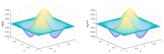
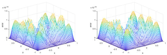
We take $\alpha =4,\beta =8,\psi (x,y)={(x^2-1)}^3{(y^2-1)}^{3}sin\left(xy\right)$. By plugging $\psi (x,y)$ into Equations (1) and (2), we can obtain $f(x,y)$. For different N, the errors between the approximate solutions and exact solutions under $L^2$ norm, 1-norm, and 2-norm are listed in Table 1. To more intuitively demonstrate the efficiency and spectral accuracy, we provide the images of the exact solution and the approximate solution in Figure 1 and the error images between them in Figure 2.

Table 1. The errors between the approximate solutions and exact solutions for different N.

N	10	15	20	25	30
$\parallel \psi -{\psi }_N\parallel$	$2.7425\times {10}^{-7}$	$3.7772\times {10}^{-15}$	$2.5901\times {10}^{-17}$	$2.9216\times {10}^{-17}$	$8.2067\times {10}^{-17}$
$\parallel \psi -{\psi }_N{\parallel }_{1,\Omega }$	$6.4867\times {10}^{-6}$	$2.8978\times {10}^{-14}$	$1.8351\times {10}^{-16}$	$2.0932\times {10}^{-16}$	$6.1571\times {10}^{-16}$
$\parallel \psi -{\psi }_N{\parallel }_{2,\Omega }$	$8.5467\times {10}^{-5}$	$1.8442\times {10}^{-12}$	$1.8625\times {10}^{-15}$	$1.9914\times {10}^{-15}$	$4.9614\times {10}^{-15}$

Figure 1. Comparison between the exact solution (left) and approximation solution (right) with N = 35.

Figure 2. The error images between the exact solution $\psi (x,y)$ and approximation solution ${\psi }_N(x,y)$ with N = 20 (left) and N = 35 (right).

It can be observed from Table 1 that the approximation solution arrives at about ${10}^{-15}$ with $N\ge 20$. In Figure 1 and Figure 2, we also observe that our algorithm is convergent, and it reaches about ${10}^{-15}$ accuracy under $L^{\infty }$ norm.

Example 2. 

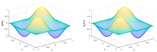
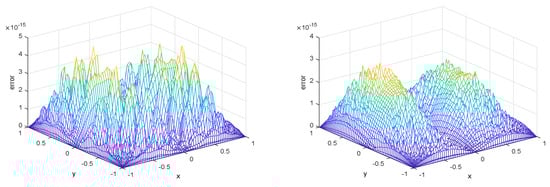
We take $\alpha =sin(x+y)+2,\beta =e^{x+y},\psi (x,y)=sin\left(\pi x\right)sin\left(\pi y\right)$. Likewise, putting $\psi (x,y)$ into Equations (1) and (2), we can obtain $f(x,y)$. For different N, the errors between the approximate solutions and exact solutions under $L^2$ norm, 1-norm, and 2-norm are listed in Table 2. We also provide the images of the exact solution and the approximate solution in Figure 3 and the error images between them in Figure 4.

Table 2. The errors between the approximate solution and exact solution.

N	10	15	20	25	30
$\parallel \psi -{\psi }_N\parallel$	$1.2534\times {10}^{-5}$	$4.8981\times {10}^{-11}$	$1.3900\times {10}^{-15}$	$5.9664\times {10}^{-16}$	$9.4303\times {10}^{-16}$
$\parallel \psi -{\psi }_N{\parallel }_{1,\Omega }$	$2.8380\times {10}^{-4}$	$1.7303\times {10}^{-10}$	$4.3041\times {10}^{-14}$	$3.3750\times {10}^{-15}$	$5.0537\times {10}^{-15}$
$\parallel \psi -{\psi }_N{\parallel }_{2,\Omega }$	0.0033	$2.0325\times {10}^{-8}$	$9.6800\times {10}^{-13}$	$3.1546\times {10}^{-14}$	$3.2913\times {10}^{-14}$

Figure 3. Comparison images of the exact solution (left) and approximation solution (right) with N = 35.

Figure 4. Error images comparing the exact solution $\psi (x,y)$ and the approximation solution ${\psi }_N(x,y)$ with N = 20 (left) and N = 35 (right).

It can be observed from Table 2 that the approximation solution arrives at about ${10}^{-13}$ accuracy with $N\ge 20$. We can also observe from Figure 3 and Figure 4 that our algorithm is convergent and arrives at about ${10}^{-15}$ accuracy under $L^{\infty }$ norm.

6.2. Three-Dimensional Resource Problem

Example 3. 

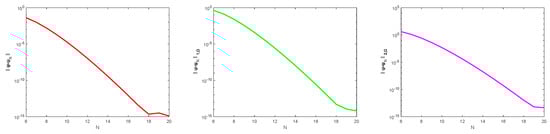
We take $\alpha =1,\beta =1,\psi (x,y)={(x^2-1)}^3{(y^2-1)}^3{(z^2-1)}^3{e}^{x+y+z}$. For different N, the errors between the approximate solutions and exact solutions under $L^2$ norm, 1-norm, and 2-norm are listed in Table 3. In addition, we also provide the error figures under three norms in Figure 5.

Table 3. The errors between the approximate solutions and the exact solutions for different N.

N	10	12	14	16	18
$\parallel \psi -{\psi }_N\parallel$	$1.8513\times {10}^{-5}$	$1.0605\times {10}^{-7}$	$3.5720\times {10}^{-10}$	$7.9225\times {10}^{-13}$	$2.4289\times {10}^{-15}$
$\parallel \psi -{\psi }_N{\parallel }_{1,\Omega }$	$3.8568\times {10}^{-4}$	$2.7105\times {10}^{-6}$	$1.0828\times {10}^{-8}$	$2.7807\times {10}^{-11}$	$5.0200\times {10}^{-14}$
$\parallel \psi -{\psi }_N{\parallel }_{2,\Omega }$	0.0047	$3.8446\times {10}^{-5}$	$1.7694\times {10}^{-7}$	$5.1558\times {10}^{-10}$	$1.0312\times {10}^{-12}$

Figure 5. Error figures of the approximate solutions under $L^2$ norm (left), 1-norm (middle), and 2-norm (right) for different N.

It can be observed that the approximate solution achieves an accuracy of about ${10}^{-10}$ even when $N\ge 16$. In Figure 5, we observe that the algorithm is still convergent and achieves spectral accuracy for the three-dimensional case.

Example 4. 

We take $\alpha =3,\beta =sinxsinysinz+2,\psi (x,y,z)={(x^2-1)}^3{(y^2-1)}^3{(z^2-1)}^{3}sin\left(xyz\right)$. For different N, the $L^2$ norm, 1-norm, and 2-norm of the errors between the exact solutions and approximate solutions are listed in Table 4.

Table 4. The errors between the exact solutions and approximate solutions for different N.

N	10	12	14	16	18
$\parallel \psi -{\psi }_N\parallel$	$4.8359\times {10}^{-9}$	$5.9351\times {10}^{-12}$	$5.6922\times {10}^{-15}$	$3.5687\times {10}^{-17}$	$5.3367\times {10}^{-17}$
$\parallel \psi -{\psi }_N{\parallel }_{1,\Omega }$	$1.2948\times {10}^{-7}$	$1.9396\times {10}^{-10}$	$2.1964\times {10}^{-13}$	$3.5002\times {10}^{-16}$	$3.3728\times {10}^{-16}$
$\parallel \psi -{\psi }_N{\parallel }_{2,\Omega }$	$1.9575\times {10}^{-6}$	$3.4997\times {10}^{-9}$	$4.6127\times {10}^{-12}$	$5.6601\times {10}^{-15}$	$2.4368\times {10}^{-15}$

From Table 4, we can see that the approximation solution achieves an accuracy of about ${10}^{-12}$ even when $N\ge 14$. We also observe from Figure 6 that our algorithm is still spectrally accurate in the three-dimensional variable coefficient situation.

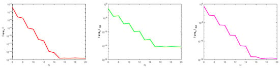
Figure 6. Error figures of the approximate solutions under $L^2$ norm (left), 1-norm (middle) and 2-norm (right) for different N.

6.3. Two-Dimensional Eigenvalue Problem

Example 5. 

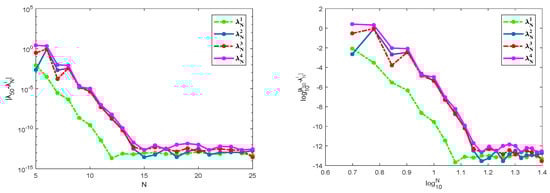
We take $\alpha =sin(x+y)+2,\beta =e^{x+y}$. For different N, the numerical results for the first four eigenvalues are presented in Table 5. In order to better demonstrate the convergence and spectral accuracy of our algorithm, we take the numerical solution of $N=50$ as a reference solution, and list the error figures of the approximate eigenvalues under the $L^{\infty }$ norm (left) and log–log scale (right) in Figure 7.

Table 5. The numerical results of the first four eigenvalues for different N.

N	${\mathit{\lambda }}_{\mathit{N}}^1$	${\mathit{\lambda }}_{\mathit{N}}^2$	${\mathit{\lambda }}_{\mathit{N}}^3$	${\mathit{\lambda }}_{\mathit{N}}^4$
5	35.2544775663993164	126.33914595504443	177.793597223306051	427.801015793001625
10	35.2460676597821418	126.34139750648265	178.093277397853029	430.41218968297477
15	35.2460676594985998	126.341393331936359	178.093272608351242	430.412179313580339
20	35.2460676594985713	126.341393331936658	178.093272608351157	430.412179313579088
25	35.2460676594986495	126.341393331936516	178.093272608351043	430.412179313579827

Figure 7. Error figures between the numerical solution and reference solution under the $L^{\infty }$ norm (left) and log–log scale (right).

It can be seen from Table 5 that the first four eigenvalues achieve accuracies of at least 14 digits when $N\ge 20$. We can observe from Figure 7 that our algorithm can converge and achieve spectral accuracy.

7. Conclusions

We developed a numerical method based on the approximation of higher-order Legendre polynomials and a rigorous error analysis for fourth-order problems under SSP boundary conditions and variable coefficients. We have theoretically obtained the existence and uniqueness of solutions and approximations, as well as the error estimation between them. In addition, we have established an effective algorithm for solving the discrete problem, which guarantees the sparsity of the mass and stiffness matrices under constant coefficient conditions. Regarding variable coefficients, we can also use the preconditioned iterative method to effectively solve the problem. The theoretical analysis and algorithms proposed in this paper can be combined with spectral element methods to tackle some nonlinear fourth-order problems in general domains, such as the Cahn–Hilliard model and transmission eigenvalue problems, among others. These represent our future research goals.

References

- Li, D.; Qiao, Z. On the stabilization size of semi-implicit Fourier-spectral methods for 3D Cahn–Hilliard equations. Commun. Math. Sci. 2017, 15, 1489–1506. [Google Scholar] [CrossRef]
- Liu, F.; Shen, J. Stabilized semi-implicit spectral deferred correction methods for Allen-Cahn and Cahn-Hilliard equations. Math. Methods Appl. Sci. 2015, 38, 4564–4575. [Google Scholar] [CrossRef]
- Shen, J.; Yang, X. Numerical approximations of Allen-Cahn and Cahn-Hilliard equations. Discret. Contin. Dyn. Syst. 2010, 28, 1669–1691. [Google Scholar] [CrossRef]
- Cahn, J.W.; Hilliard, J.E. Free energy of a nonuniform system. I. Interfacial free energy. J. Chem. Phys. 1958, 28, 258–267. [Google Scholar] [CrossRef]
- Michelson, D.M.; Sivashinsky, G.I. Nonlinear analysis of hydrodynamic instability in laminar flames-II. Numerical experiments. Acta Astronaut. 1977, 4, 1207–1221. [Google Scholar] [CrossRef]
- Sivashinsky, G.I. Nonlinear analysis of hydrodynamic instability in laminar flames-I. Derivation of basic equations. Acta Astronaut. 1977, 4, 1177–1206. [Google Scholar] [CrossRef]
- Canuto, C. Eigenvalue approximations by mixed methods. RAIRO. Anal. Numrique 1978, 12, 27–50. [Google Scholar] [CrossRef]
- Rappaz, J.; Mercier, B.; Osborn, J.; Raviart, P.A. Eigenvalue approximation by mixed and hybrid methods. Math. Comput. 1981, 36, 427–453. [Google Scholar]
- Chen, W.; Lin, Q. Approximation of an eigenvalue problem associated with the stokes problem by the stream function-vorticity-pressure method. Appl. Math. 2006, 51, 73–88. [Google Scholar] [CrossRef]
- Yang, Y.D.; Jiang, W. Upper spectral bounds and a posteriori error analysis of several mixed finite element approximations for the stokes eigenvalue problem. Sci. China Math. 2013, 56, 1313–1330. [Google Scholar] [CrossRef]
- Sousa, E. An explicit high order method for fractional advection diffusion equations. J. Comput. Phys. 2014, 278, 257–274. [Google Scholar] [CrossRef]
- Liu, Y.; Du, Y.; Li, H.; He, S.; Gao, W. Finite difference/finite element method for a nonlinear time-fractional fourth-order reaction-diffusion problem. Comput. Math. Appl. 2015, 70, 573–591. [Google Scholar] [CrossRef]
- Canuto, C.; Hussaini, M.Y.; Quarteroni, A.; Zang, T.A. Spectral Methods: Evolution to Complex Geometries and Applications to Fluid Dynamics; Springer: New York, NY, USA, 2007. [Google Scholar]
- Guo, B.Y.; Jia, H.L. Spectral method on quadrilaterals. Math. Comput. 2010, 79, 2237–2264. [Google Scholar]
- Guo, B.Y.; Wang, L.L. Error analysis of spectral method on a triangle. Adv. Comput. Math. 2007, 26, 473–496. [Google Scholar] [CrossRef]
- Boyd, J.P. Chebyshev and Fourier Spectral Methods; Courier Corporation: Chelmsford, MA, USA, 2001. [Google Scholar]
- Bialecki, B.; Karageorghis, A. A Legendre spectral Galerkin method for the biharmonic Dirichlet problem. SIAM J. Sci. Comput. 2001, 22, 1549–1569. [Google Scholar] [CrossRef]
- Zhuang, Q. A Legendre spectral-element method for the one-dimensional fourth-order equations. Appl. Math. Comput. 2011, 218, 3587–3595. [Google Scholar] [CrossRef]
- Li, L.; An, J. An efficient spectral method and rigorous error analysis based on dimension reduction scheme for fourth order problems. Numer. Methods Partial Differ. Equ. 2021, 37, 152–171. [Google Scholar] [CrossRef]
- Shen, J. Efficient spectral-Galerkin method I. Direct solvers of second-and fourth-order equations using Legendre polynomials. SIAM J. Sci. Comput. 1994, 15, 1489–1505. [Google Scholar] [CrossRef]
- Shen, J. Efficient spectral-Galerkin method II. Direct solvers of second-and fourth-order equations using Chebyshev polynomials. SIAM J. Sci. Comput. 1995, 16, 74–87. [Google Scholar] [CrossRef]
- Eftekhari, T.; Rashidinia, J. A new operational vector approach for time-fractional subdiffusion equations of distributed order based on hybrid functions. Math. Methods Appl. Sci. 2023, 46, 388–407. [Google Scholar] [CrossRef]
- Chen, L.; An, J.; Zhuang, Q. Direct solvers for the biharmonic eigenvalue problems using Legendre polynomials. J. Sci. Comput. 2017, 70, 1030–1041. [Google Scholar] [CrossRef]
- Aslefallah, M.; Shivanian, E. Nonlinear fractional integro-differential reaction-diffusion equation via radial basis functions. Eur. Phys. J. Plus 2015, 130, 47. [Google Scholar] [CrossRef]
- Shivanian, E.; Aslefallah, M. Stability and convergence of spectral radial point interpolation method locally applied on two-dimensional pseudoparabolic equation. Numer. Methods Partial Differ. Equ. 2017, 33, 724–741. [Google Scholar] [CrossRef]
- Aslefallah, M.; Abbasbandy, S.; Shivanian, E. Numerical solution of a modified anomalous diffusion equation with nonlinear source term through meshless singular boundary method. Eng. Anal. Bound. Elem. 2019, 107, 198–207. [Google Scholar] [CrossRef]
- Aslefallah, M.; Yüzbaşi, Ş.; Abbasbandy, S. A Numerical Investigation Based on Exponential Collocation Method for Nonlinear SITR Model of COVID-19. CMES-Comput. Model. Eng. Sci. 2023, 136, 1687–1706. [Google Scholar] [CrossRef]
- Bernardi, C.; Maday, Y. Spectral methods. Handb. Numer. Anal. 1997, 5, 209–485. [Google Scholar]
Disclaimer/Publisher’s Note: The statements, opinions and data contained in all publications are solely those of the individual author(s) and contributor(s) and not of MDPI and/or the editor(s). MDPI and/or the editor(s) disclaim responsibility for any injury to people or property resulting from any ideas, methods, instructions or products referred to in the content. |
© 2023 by the authors. Licensee MDPI, Basel, Switzerland. This article is an open access article distributed under the terms and conditions of the Creative Commons Attribution (CC BY) license (https://creativecommons.org/licenses/by/4.0/).