Abstract
Robust learning is an important issue in Scientific Machine Learning (SciML). There are several works in the literature addressing this topic. However, there is an increasing demand for methods that can simultaneously consider all the different uncertainty components involved in SciML model identification. Hence, this work proposes a comprehensive methodology for uncertainty evaluation of the SciML that also considers several possible sources of uncertainties involved in the identification process. The uncertainties considered in the proposed method are the absence of a theory, causal models, sensitivity to data corruption or imperfection, and computational effort. Therefore, it is possible to provide an overall strategy for uncertainty-aware models in the SciML field. The methodology is validated through a case study developing a soft sensor for a polymerization reactor. The first step is to build the nonlinear model parameter probability distribution (PDF) by Bayesian inference. The second step is to obtain the machine learning model uncertainty by Monte Carlo simulations. In the first step, a PDF with 30,000 samples is built. In the second step, the uncertainty of the machine learning model is evaluated by sampling 10,000 values through Monte Carlo simulation. The results demonstrate that the identified soft sensors are robust to uncertainties, corroborating the consistency of the proposed approach.
MSC:
68T01; 68T07; 65C05; 90B30
1. Introduction
Machine learning (ML) has been widespread in several application domains. Hence, this has given birth to a new field of study: Scientific Machine Learning (SciML). This field is concerned with the proper application of an ML model by taking into consideration all peculiarities of a given domain. As ML becomes more popular, several concerns have arisen [1,2,3,4,5]. It is possible to find recent work in the literature concerned with developing uncertainty-aware ML models [6,7]. These works seek to provide viable methods to evaluate the prediction uncertainty of the models. However, the literature still lacks a methodology for evaluating all the sources of uncertainty surrounding ML model identification and prediction. Uncertainty is an important topic, as developing robust models is essential for applying an ML in a real-case scenario. Most application domains have associated uncertainties caused by corrupted data, measurement noise, redundancies, and instrument uncertainties. Hariri et al. [8] discuss how uncertainty can impact big data in terms of analysis and the dataset. They show that if the learning algorithm uses corrupted training data, it will likely produce inaccurate results. When these issues are not considered, the ML tools may perform poorly and become inadequate. This might create general scepticism in the general scientific community towards ML tools. Hence, robust learning plays an essential role in the SciML literature.
Despite its increasing interest, there are still a lack of algorithms that efficiently cope with the epistemic and aleatory uncertainties in real case scenarios [6,9]. For instance, Gal and Ghahramani [10] present a seminal work regarding this topic. The authors proposed evaluating reinforcement learning models using a Bayesian approximation technique. The referred article points toward issues that still needs to be addressed in this field. Some of these issues are addressed in the present work.
Fully understanding the uncertainty of ML models is still a complex issue, as it means evaluating the uncertainty of predictions. Similar approaches in different fields have been proposed to address uncertainty analysis of model prediction [11,12]. For instance, Gneiting, Tilmann; Balabdaoui, Fadoua; Raftery [13] propose an efficient method to calibrate the distribution of a known random variable. This work addresses the issues related to non-deterministic variables and their effect on model prediction. Abdar et al. [14] and Siddique et al. [15] present comprehensive reviews of this topic and reinforce the increasing necessity for further development. Costa et al. [16] propose a novel strategy for developing uncertainty-aware soft sensors based on a deep learning architecture. The authors mention the need for developing methods that simultaneously evaluate the different uncertainty components involved in an ML model identification. Table 1 compares different methods for evaluating uncertainty in neural networks based on the work of Abdar et al. [14].

Table 1.
Comparison of methods for quantifying uncertainty.
While identifying an ML model, several perspectives must be considered. For instance, Abdar et al. [14] proposed three primary uncertainties related to an ML application, the absence of theory and causal models, the sensitivity to data corruption or imperfection, and the computational effort. Levi et al. [17] proposed a simple recalibration method that significantly improves real-world applications. However, they indicate that further work is needed to test the method’s generalizability. Levi et al. [17] also assume that the prediction is a known distribution. As mentioned, several methodologies in the literature address one of these listed points. However, the literature lacks methods to address them in the same framework. Additionally, Abdar et al. [14] present some methods for quantifying uncertainty, i.e., bootstrapping and ensemble. On the other hand, in identifying soft sensors for real-time applications, the computational cost associated with the calculations can make their use infeasible.
Hence, this work proposes a comprehensive methodology for uncertainty evaluation of an ML model for SciML. The proposed method considers the epistemic and aleatory uncertainties related to both data used to train the models and the models themselves. Therefore, it is possible to provide an overall strategy for uncertainty-aware models in the SciML field. This work contributes to the robust learning literature as it allows for an approach that considers the several sources of uncertainty involved in SciML model identification. The proposed methodology uses Bayesian inference to evaluate non-linear models’ uncertainty propagation for ML models through Monte Carlo methods.
The following sections of this work present the proposed methodology and a case study with soft sensors for a polymerization reactor. Thus, Section 2 presents the methodology, Section 3 is the results and discussions, Section 4 presents the conclusions, and supplementary information on the results is shown in Appendix A.
2. Methodology for Monte Carlo Uncertainty Training
This paper proposes a general methodology to build surrogate models based on artificial intelligence (AI) with uncertainty assessment. The proposed methodology is divided into five steps to obtain the validated machine learning models with uncertainty assessment. Figure 1 presents the general scheme of the proposed method as follows.
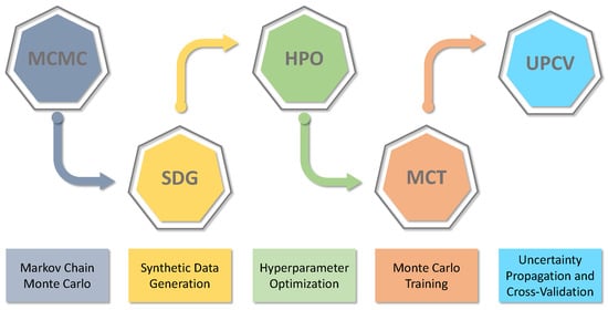
Figure 1.
General methodology scheme.
The first step is to use the Markov Chain Monte Carlo method to obtain the uncertainty of the non-linear model parameters that represent the system. Following the methodology, the validated model is used to generate synthetic data. These synthetic data are used to build the neural networks in two steps. The first step is to define the type and the general architecture of the neural network before optimising the hyperparameters. After finding the best network architecture, the second step is to perform Monte Carlo simulation training to propagate the uncertainty from the non-linear model (i.e., synthetic data) to the AI model. The last step of the proposed methodology is to perform validation and uncertainty assessment of the trained model. In that step, the AI model prediction and simulation are collated with the non-linear model and experimental data when available. Further, uncertainty assessment is performed with the appropriate hypothesis in that step. The following subsections provide specific details about each stage of the proposed methodology.
2.1. Markov Chain Monte Carlo
Phenomenological and empirical models have common parameters that interfere with their respective output behaviour. In these models, parameter estimation is a challenge because their choice contributes to the prediction uncertainty of the model. Consider a non-linear dynamic model written as:
where is the relationship function between the time t, states , the input vector , parameters , and the output vector . In this scenario, if is a set of parameters. If they have a low predictive probability, the model will not provide a good forecast or adjustment to experimental data [18]. Thence, it is essential to know the model’s parameter probability density function (PDF) and, consequently, the model uncertainty to ensure that the model and the parameters are good enough.
Several methods are available in the literature to solve the inference problem and to estimate parameters and the associated uncertainty. Bard [19] presents several tools to obtain the variance of models from the frequentist approach, including the Least Squares and Maximum Likelihood methods. The main drawback of the Bard [19] methods is the hypothesis imposed to obtain the variance of the parameters, including Gaussian distribution. However, the Bayesian approach estimates the joint probability distribution using all available information about the system without assumptions about the target distribution [20].
The Bayesian approach to inference allows obtaining the posterior PDF of any set of parameters using as information the inferred data and any previous information about the system . Therefore, using the Bayes Theorem, it is possible to write the following relationship between the earlier variables [20]:
where represents sampled values of , L is the likelihood function, and is the prior distribution of that is a new observation of . Equation (2) allows updating the actual knowledge of the system represented by the posterior .
The likelihood is defined by Migon et al. [18] as a function that associates the value of the probability with each value. By defining the estimation process as a least square problem, the objective is to minimize a loss function that can be represented by a weighted least square estimator (WLSE). Thus, the likelihood function can be defined as:
where is the residual between the experimental data and that obtained with the prediction model . Further, the use of the WLSE estimator implies the use of the variance of the residual between the and for the outputs of the system, represented in Equation (3) as .
The posterior PDF of each parameter of the vector , is obtained from the marginal posterior density function and is defined by Gamerman and Lopes [20] as:
Chapter 5 by Gamerman and Lopes [20] presents several methods for solving the inference problem of Equation (4). The Markov Chain Monte Carlo methods have some interesting features among the numerical integration methods. Among these characteristics is convergence, because when chains are adequately constructed, after a sufficiently high number of iterations, the chains converge to an equilibrium distribution. Thus, Figure 2 shows a schematic diagram of the solution to the inference problem using the MCMC method. The general idea is that the MCMC uses existing information, such as experimental data and a likelihood function, to provide a mathematical model and the associated PDF of the estimated parameters.
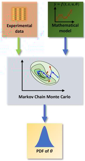
Figure 2.
MCMC method.
On the other hand, this paper proposes using the DRAM (Delayed Rejection Adaptive Metropolis) MCMC algorithm Haario et al. [21] presented to solve the inference problem. The DRAM algorithm combines the Adaptive Metropolis, which provides global adaptation, and the Delayed Rejection, which offers local adaptation. Further, the main idea of the DRAM algorithm is to collect information during the chain run and tune the target PDF by using the learned information.
2.2. Synthetic Data Generation
In building AI models, data quality is crucial to obtain great adjusted models. This paper proposes a methodology to build AI models using synthetic data from a non-linear model. Further, the methodology is based on the uncertainty propagation law established in BIPM et al. [22], Bipm et al. [23], BIPM et al. [24]. In this sense, the quantity and quality of data used in training must be adequate, which means the inputs must be uncorrelated and the amount of data needs to be enough to provide information to the training process. Then, Section 3.1 and Section 3.4.2 present results that illustrate this issue by providing numerical information regarding the adequate amount of data and distribution and input features. It is important to highlight that the inadequate use of data can lead to underestimation of uncertainty. Such a situation can undermine the uncertainty assessment.
This paper proposes to build a training database by drawing a sample of the parameters of PDF and propagating it to the outputs of the non-linear model. In this way, the data used for training the models need to be representative of the operating conditions of the system and characterize the uncertainties of the non-linear model. Figure 3 presents a generic Monte Carlo Method (MCM) simulation scheme for synthetic data generation. The scheme in Figure 3 is inspired by the algorithm for implementing the Monte Carlo Method presented in Supplements 1 and 2 and to the “Guide to the expression of uncertainty in measurement” [22,24].
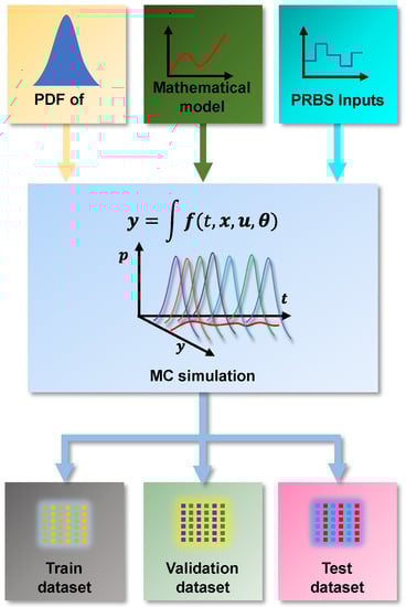
Figure 3.
Monte Carlo simulation method for data generation.
The first step of the algorithm is to determine the number m of trials to be performed. In general, the MCM produces better responses with a greater number of shots, and the recommendation is to use a value [18]. However, smaller values can be used when evaluating complex models requiring high computational costs for numerical solutions. This reduction in the number of tests may not allow the correct characterization of the PDF of the output values and may produce less reliable results [22].
After defining the number of tests to be performed, a matrix containing m vectors of PDF samples of is built:
Thus, m distinct sets of model parameters are obtained such that it is possible to write
in this way, it is possible to integrate the model so that the m dynamic responses are obtained for the output variables y.
As it is a dynamic model, it is necessary to obtain representative data from the entire operating region. An independent Pseudo-Random Binary Sequence (PRBS) signal for each of the inputs is generated through a Latin Hypercube Sampler (LHS). The PRBS signals are then combined with the non-linear mathematical model of the system. A dynamic response is received for each parameter combination obtained from the PDF of the parameters. Additionally, the system’s dynamic response is represented by a set of curves obtained from this MC simulation. In this scenario of propagation of uncertainties by MCM in dynamical systems, the true value must be calculated for each sampling instant in which the equations are solved. In this way, it is considered that for each sampling instant, a PDF sample is obtained for each system output response .
From Figure 3, it is also possible to observe that the data generated through the MC simulation will be divided into three sets: training, testing, and validation. This division follows the common literature guidelines for training AI models [25]. The first two sets are used during supervised training of the models, since the algorithms need two data sets for training and validation. The third set, the test dataset, is used for final cross-validation as these data are “unknown” to the AI model. Thus, the ability to predict and extrapolate to new data is evaluated. Additionally, dividing the data into three sets must consider that the training process has consistent information. In this sense, sets are typically divided into: Train—70%, Validate—15%, and Test—15%.
2.3. Data Curation
A database to train a dynamic data-driven model should be systematically organized to represent the system dynamics. Hence, the identified model can approximate the observed dynamic phenomena. There are several ways to manage a data set to incorporate the system’s time dependence. The most common is non-linear autoregressive with exogenous inputs (NARX) predictors. The general NARX structure is composed of a prediction of the actual output as:
where is the input delay, and are the p of past values for the output and input, respectively. The noise, , is additive: for the NARX, the error information is assumed to be filtered through the system’s dynamic. In its turn, is a parameter that represents the model parameters’ uncertainty. As observed from Equation (7), the NARX predictor has two hyperparameters: n and p. These parameters should be defined correctly to improve the dynamic representativeness of the data. For this purpose, He and Asada [26] proposed the Lipschitz coefficient analysis. A Lipschitz coefficient is then calculated for each pair of measurements. For further information about the Lipschitz coefficient calculations, see He and Asada [26].
2.4. Building the AI Model
Figure 4 shows a methodology step responsible for finding the hyperparameters of the network. That step defines the appropriate architecture and network format that one wants to get before starting the training. The type of network is the first aspect to be evaluated when building an AI model. In this way, expert knowledge must be considered to define whether a network is to be used, e.g., recurrent, convolutional, or dense. Choosing the network format depends on the characteristic of the system being modelled and the main application of the model.
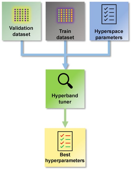
Figure 4.
Optimization procedure to find the hyperparameters of the neural network.
Once the general format of the type of network is defined, the next step is to define its architecture. There are some powerful algorithms available in the literature for this means. The optimal number of layers determines the architecture of a neural network, the number of neurons per layer, and activation functions, among other parameters [27]. Determining these parameters is one source of uncertainty during the modelling process that needs to be considered.
2.5. Monte Carlo Training
The fourth step of the methodology proposed in this work is the uncertainty training of networks through Monte Carlo simulations. The stages of generating data, obtaining the architecture of the neural network, and the hyperparameters provide the necessary information for the uncertainty training of the networks. In this way, it is sought to characterize the prediction region of the identified non-linear system, obtained in Section 2.1, through a set of networks capable of representing each of the probable outputs of the model.
Figure 5 presents a simplified schematic diagram of this step in the methodology. It is possible to observe that the MC training stage boils down to massive training on top of the generated data. The result is a set of equally probable trained AI models that comprehensively account for the uncertainty sources.
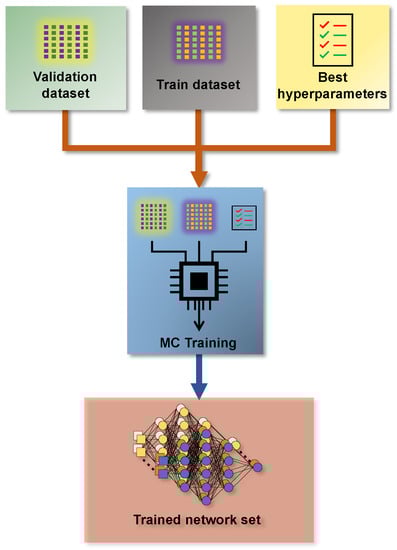
Figure 5.
Monte Carlo training method.
This training step follows the concepts of Monte Carlo simulations. It is the step that has the most significant computational effort. The simulation is built to train an AI model with pre-defined optimal architecture for each element in the training, validation, and test datasets. In addition to the computational effort required to perform this step, the volume of data generated is also significant. However, the amount of data generated has a less relevant impact.
On the other hand, nowadays, SciML model training has become increasingly efficient. The literature has presented algorithms that extract maximum performance from the available hardware. Additionally, manufacturers have built hardware with specific characteristics for application training and execution of artificial intelligence. In this scenario, the available technology makes it feasible to run a Monte Carlo simulation for training neural networks. The proposed method obtains the network uncertainty by a set of identically retrained networks. Therefore, the predicted most likely value is obtained through the expectation of all networks set at each instant. Then, the Monte Carlo training step allows for obtaining the necessary network parameters to perform the prediction.
2.6. Propagation and Cross-Validation
The methodology proposed in this article includes a supplementary validation stage of the built AI model. In this step, the data used for cross-validation are labelled “Test data” in Figure 3 (Note that the set called “validation” is used during training). In a complementary way, validation in the context of dynamic models with uncertainty needs to be evaluated to compare the coverage regions. In this context, a model is considered validated when the coverage of regions of models is overlapping, implying that the values are statistically equal.
The main issue involved is the method used to assess the uncertainty of the model. For both the non-linear phenomenological model and the AI model, this article proposes to use the Monte Carlo method. Thus, the uncertainty of the evaluated model can be obtained assuming the same hypotheses proposed by Haario et al. [21,28]; that is: the variance is approximated by an inverse Gamma distribution. Then:
where the distribution is supported in and represented by , and the and parameters are the shape and scale of the distribution, respectively.
In turn, to obtain the parameters and , Gelman et al. [29] suggest using:
where is the number of outputs of the model. On the other hand, is the variance of the prior, and is the sum of the squared errors between the prediction and the experimental data.
Using the hypothesis of a non-informative prior, the variance of the prior and the number of points are unknown. In this way, the previous equations can be approximated by:
The methodology of this article implies obtaining two sets of model parameters that each have their associated uncertainty. Thus, the proposal is that the variance calculation is performed using the SSE obtained through the estimation data when the MCMC is performed. The SSE is obtained with the training data for the training of networks. Then, the uncertainty of a prediction will be based on the variance of the model that will follow the inverse gamma distribution. This methodology allows for characterizing the epistemic uncertainty of the model.
3. Results and Discussion
This section presents the results of applying the proposed methodology in a case study. A polymerization reactor with synthetic data is used as a case study. The detailed polymerization model is presented in Section 3.1. Following the proposed methodology, Section 3.2 explains network construction using the Monte Carlo method, uncertainty propagation, and final cross-validation.
3.1. Case Study: Polymerization Reactor
The reactor model is presented in detail by Hidalgo and Brosilow [30], Alvarez and Odloak [31]. It is composed of a system of algebraic differential equations (DAE) with thirteen equations as follows:
In the above DAE system, Equations (13)–(16) represent the mass and energy balance of the monomer and the initiator. Equations (17)–(19) are the moment equations of the dead polymer, in which , , and represent the moments of the dead polymer. Algebraic equations are used to describe the relationship between supplementary variables. Equation (22) represents the weight-average molecular weight, and Equation (24) represents the viscosity. Table 2, Table 3 and Table 4 show the model parameters general definitions, the initial condition values of inputs, and the steady-state output system variables.
Table 2.
Parameters and initial conditions.
Table 3.
Steady-state input conditions and LHS region.
Table 4.
Output variables at steady-state.
Alvarez and Odloak [31] developed this model based on seven hypotheses: the lifetime of the radical polymer is shorter than that of other species; Long Chain Assumption (LCA) is related to monomer consumption; the chain transfer reaction to monomer and solvent can be neglected; operation below 373 K because greater temperatures cause monomer thermal initiation; termination by disproportionation is not considered; the rate of termination is dominant; and only the heat of polymerization is considered.
Alvarez and Odloak [31] discuss the polymerization reactor from the control and optimization point of view. However, other relevant aspects are pointed out. One of these, Alvarez and Odloak [31], uses Equation (23) as a virtual analyser for the viscosity because this is a difficult variable to measure in the studied reactor. The authors use the temperature and the viscosity as controlled variables, manipulating the initiator flow rate and the rate of the cooling jacket. Therefore, this case study is used to validate the proposed methodology for the uncertainty assessment of neural networks. Further, using an AI model reduces the computational efforts of the control and optimization loops.
As no experimental data are available regarding this system, this paper proposes using random white noise to simulate the interferences that usually occur in an experimental setup. The system is simulated with the initial and steady-state conditions in Table 2 and Table 3, respectively.
Figure 6 shows the LHS generated with % of the steady-state input value and used as input in the simulation. A total of 30 steps, with 150 h of simulation each, were developed to compose the synthetic data.
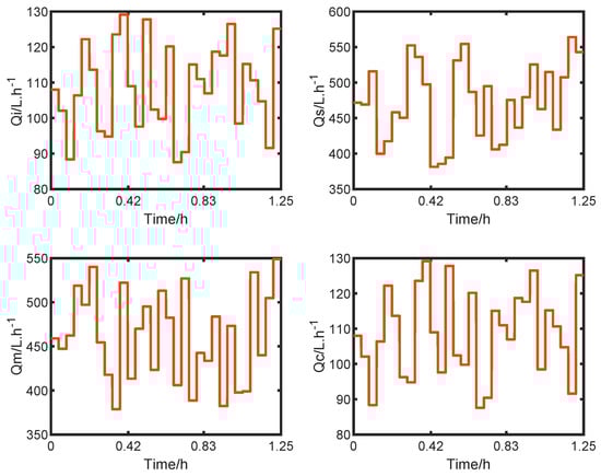
Figure 6.
LHS inputs.
Figure 7 presents the correlation heat map for the variables set by the LHS. The main diagonal presents high correlations as it pairs the variables with themselves. In contrast, the pairing between the other entries produces a value that allows verifying if the generated values are uncorrelated. The lower these values, the less correlated they are. As shown in Figure 7, the correlations are close to null, demonstrating that the LHS can efficiently generate uncorrelated samples.
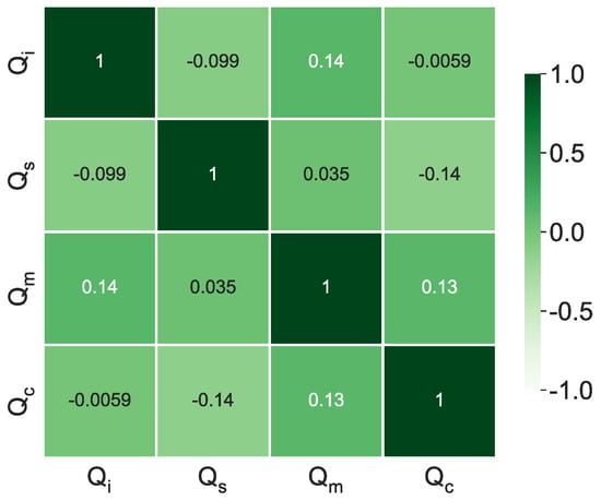
Figure 7.
Input correlation map.
The synthetic output dataset is shown in Figure 8. As mentioned, random noise with −20 dB and 10% of the output range is included in the signal to emulate the field conditions. All these variables are used in the likelihood function presented in Equation (3). A total of 70% of these data are used for the SciML model identification, and the rest are used for the methodology cross-validation step, as discussed in the subsequent sections.
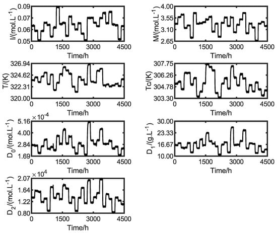
Figure 8.
Synthetic output data with white noise.
3.2. MCMC
The generated synthetic data allows the uncertainty assessment of the Alvarez and Odloak [31] model, done through the MCMC methodology. Therefore, 12 model parameters and 6 initial conditions were used as decision variables for the MCMC algorithm. The DRAM algorithm proposed by Haario et al. [21] allows limiting the parameter search region. Therefore, in this paper, the search region was limited to % of the nominal value of the parameter. Further, all parameters were normalized to the nominal value to facilitate the algorithm’s convergence.
Other algorithm aspects must be set. The first is the number of samples sorted to build the joint PDF. At this point, the algorithm was configured to build a set with 30,000 samples of the targeted joint PDF. The algorithm was also configured to use a non-informative prior. Therefore, to estimate the variance of the parameter, the algorithm chooses 5000 samples to update the prior and discards the chain. After the burn step, the MCMC algorithm restarts building the chains and evaluates the parameters in the search region.
Table 5 shows the resulting normalized parameters obtained from the Markov Chains. The MCMC algorithm does not make any assumptions about the target distribution. The mean and median in normal distributions converge to the same number. However, it is more conservative to assume that the distribution is not Gaussian and to use the median as a value for the most probable value. In Table 5, it is possible to see the difference between the parameter’s mean and median. Table 5 also shows the standard deviation (std) and the Geweke diagnostic parameter [32]. For some parameters, the std value is relatively high. However, the Geweke parameter indicates that the chain converges [32]. Figure A1–Figure A11 in the Supplementary Material (Appendix A) show the confidence region and the full Markov Chain. Those figures compare Gaussian and unshaped regions proposed by Possolo [33].
Table 5.
Normalized parameters obtained by DRAM algorithm.
The MCMC algorithm has the particularity of being unable to be parallelised. This comes from the need to carry out the random walk sequentially. In this way, this procedure implies the use of few computational resources but for a long time. Then, the algorithm sampled 72,672 sets to obtain the 30,000 samples for the posterior PDF. It used a computational time of about 76.10 h of processing on a computer with two AMD EPYC 7252 processors and 32 Gb of memory.
3.3. Synthetic Data Generation for Training
The results of the MCMC allow the construction of the parameter PDF of the phenomenological model capable of representing the uncertainty of the non-linear system. Thus, it is possible to build a set of non-linear responses by randomly selecting a set of parameters. This work randomly selected a sample of 10,000 distinct non-linear parameters. Subsequently, all resulting models were excited with the same LHS signal as in Figure 6, and the result was 10,000 different dynamic responses.
With these dynamic trajectories, it was possible to establish the number of embedded dimensions of the NARX model. The Lipschitz method is presented in Section 2.3 and was used to define the NARX parameters. Figure 9a,b show these results. In Figure 9a,b, the decisive factor is the slope of the surface, because when there is high variation between two delays, the increase is considered important. However, if the slope variation is low, it can be considered that this inclusion is not necessary. Then, it is possible to observe that a delay of four sampling instants for the inputs and one for the variables is reasonable for good representation, as after these values, the slope starts to be constant.
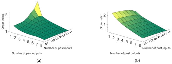
Figure 9.
(a) Lipschitz surface for reactor temperature; (b) Lipschitz surface for polymer viscosity.
3.4. Monte Carlo Training
The proposed methodology includes a step called ’Monte Carlo training’, which is composed of smaller steps. It starts with the identification of the hyperparameters. It is followed by defining the data needed for training. Then, finally, the final Monte Carlo training is done.
3.4.1. Monte Carlo Training
The network’s optimal structure is found by a search in a hyperspace formed by the structural parameters that constitute the networks. Table 6 shows the initial configuration included in the hyperband algorithm [27].
Table 6.
Hyperband hyperspace search.
The results obtained from the hyperparameter search are presented in Table 7. It is possible to observe that a relatively simpler network was necessary to represent the temperature than the viscosity. This simpler architecture implies a big difference in the computational cost. The viscosity network required 6.4 times longer to be trained than the network for the temperature. On the other hand, the networks have the same activation functions in the layers and the same learning rate. Table 7 also shows the MAE and MSE values resulting from the hyperband search. The hyperband algorithm uses the training and validation datasets during training. Then, the test dataset is used after the training to test the final model parameters. It is noteworthy, however, that this methodology assumes that the network’s architecture does not change to a variable. In this way, it is considered that it is only necessary to execute the hyperparameter search process once. With the network structure identified, it is trained for all trajectories obtained from each non-linear model. Hence, a set of networks is identified, as described in Section 2.5.
Table 7.
Resulting network hyperparameters.
3.4.2. Data Size
An important aspect to be analysed in neural network training is the guarantee of adequate training. In this sense, assessing whether the amount of information added in training the model is sufficient for the training algorithm to obtain a suitable model is necessary. Figure 10 shows this analysis for the polymer viscosity and reactor temperature. This evaluation was based on a set of independent training sets in which each one was repeated 25 times. The first 25 training sets were carried out with 100 experiments. The average values for MAE and the final MSE were calculated. For the next 25, 100 experiments were added, and so on. In Figure 10, it is possible to observe that for viscosity, after about 1750 experiments, there is no significant change in the MSE; however, for MAE, this value is about 1500. On the other hand, when the reactor temperature is evaluated, this value is higher, and more than 2500 experiments were needed for convergence. Thus, to ensure convergence, 3100 were used for both networks.
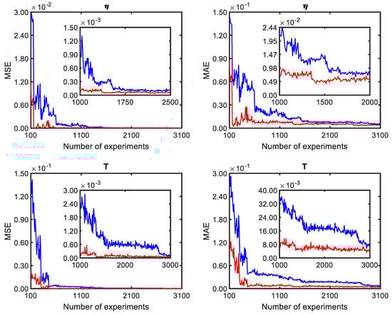
Figure 10.
Training performance as a function of experiments.
3.4.3. Training
The adaptive moment estimation algorithm (ADAM) proposed by [34] was used to train the chosen structure. ADAM is an optimization method based on the descending gradient technique, making the ADAM algorithm efficient for problems involving extensive data and parameters. It also requires less memory than other training algorithms because the data are sliced into several packages and treated.
Building the networks involves an exhaustive training process called ’Monte Carlo training’. The proposed methodology is based on the Monte Carlo method for PDF propagation. Thus, the assumed hypothesis is that the different trajectories generated through the non-linear model can represent the model’s uncertainty. Therefore, training networks capable of representing these distinct trajectories imply obtaining a PDF of trained parameters of an AI model that also represents the uncertainty of the model.
Convergence analysis of training networks via MC training can be performed by analysing MAE and MSE values similar to conventional training. However, given the number of trained networks, it is more convenient to evaluate in histogram format, as in Figure 11. In the first analysis, Figure 11 shows the histograms of the MAE and MSE indicators, both for the test and validation data. It is possible to observe that the histograms do not follow a Gaussian distribution. Thus, the mean may not be a good reference in statistical terms. Thus, Table 8 shows the minimum, maximum, median, and standard deviation of the MAE and MSE. Generally, it is possible to affirm that the networks converged sufficiently.
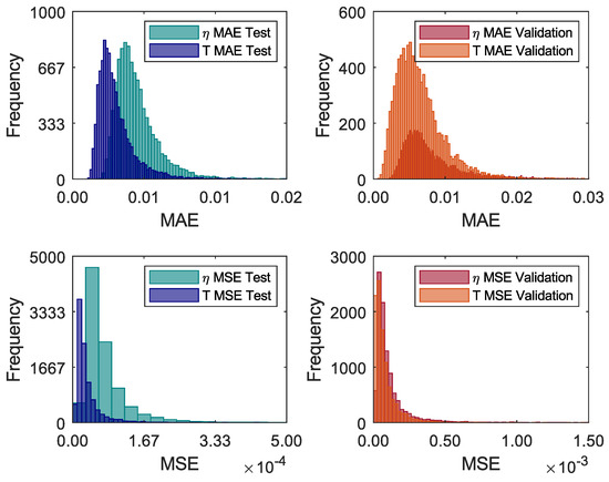
Figure 11.
Monte Carlo Training convergence evaluation.
Table 8.
Training network performance.
In the Monte Carlo Training process, an early stopping option in MC training was used to reduce the computational cost. Thus, training was aborted if there ewas no decrease in the LOSS value for 100 epochs. Figure 12 shows the histograms of the number of epochs trained during MC training for the two modelled variables. In the graph of Figure 12, the minimum number of epochs was 50, and the maximum number was 300. Lognormal distributions with lower or upper bounds should be the best representation for this data type. Figure 12 also shows that the data do not fit a lognormal distribution. Hence, no assumptions were made about the type of distribution of variables. Additionally, Figure 12 shows the distribution of each network’s time consumption during the Monte Carlo training process. With the early stopping option, the number of epochs trained is variable, and the time consumption during the training differs for each Monte Carlo trail. The training calculation through CM was performed using a computer with a dedicated Tesla T4 16 Gb GPU, two AMD EPYC 7252 processors, and 32 Gb of memory. The MC method can be parallelised when GPU processing is not used. Then, the training was carried out sequentially and totalled 155 h of training, which is the sum of all values presented in Figure 12.
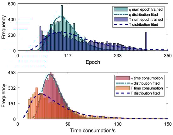
Figure 12.
Trained epochs and training time of Monte Carlo training.
3.5. Uncertainty Propagation and Validation
The last step of the proposed methodology is the propagation of uncertainty and methodology cross-validation. The proposal is based on constructing the uncertainty regions of the neural network’s prediction and comparison with the uncertainty regions of the non-linear phenomenological model. With the prediction values, it is possible to calculate the variance of the networks using the same assumptions used to calculate the uncertainty of the phenomenological model Equations (13)–(24). Figure 13 and Figure 14 show the comparisons between the predictions for the two modelled variables: T and .
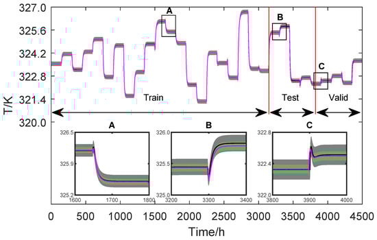
Figure 13.
Training and validation data of T.
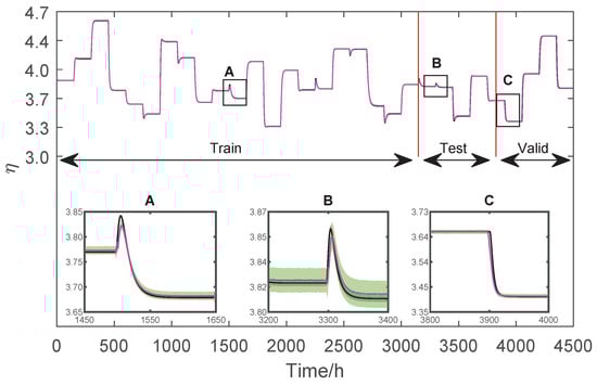
Figure 14.
Training and validation data of .
Figure 13 and Figure 14 present the entire output dataset used for training, testing, and validation. A zoom is given to verify the variables’ behaviour in each region. It is pointed out, however, that the training and validation data sets are used during the training of the networks. In this way, the networks’ only unknown is the test data set, which is used to certify their performance.
From a statistical point of view, when two measurements have overlapping coverage regions, they are impossible to differentiate, and they are considered equal. Therefore, validation of the AI model against the non-linear phenomenological model is achieved when the dynamic range regions are superimposed. In this sense, the graphs of Figure 13 and Figure 14 allow us to conclude that both models statistically produce the same dynamic response.
4. Conclusions
This work presented a novel methodology for evaluating the uncertainty of Scientific Machine Learning Models. A comprehensive approach was proposed that considered several uncertainties associated with the SciML model structure, the data used, and the original data source. The proposed strategy was composed of five steps: Markov Chain Monte Carlo method to obtain the uncertainty of the non-linear model parameters; generation of synthetic data; neural network structure identification; Monte Carlo simulation training; and methodology validation and uncertainty assessment of the trained mode.
The proposed method considers epistemic and aleatory uncertainties. These uncertainties are considered in the context of the data used to train the models and the model itself. Therefore, it is possible to provide an overall strategy for the uncertainty-aware models in the SciML field. The proposed approach can be applied to different ML models for numerical data prediction. On the other hand, it is not applied to categorical or image classification ML. This limitation exists, as it requires methods that allow quantifying the uncertainty of categorical variables and classification. Another limitation of this method is the computing effort required by it. This issue limits its application in online learning, as the computational effort can make the application unfeasible. This last limitation should be a topic of further development of the proposed methodology.
A case study demonstrated the method’s consistency. Hence, two soft sensors were identified to provide information about the temperature and viscosity of a polymerization reactor. The results indicated that the soft sensor predictions are statistically equal to the validation data in both dynamic and stationary regimes. Therefore, a practical implication of the proposed method is that, for the prediction and evaluation of uncertainty in real-time applications, the computational cost is not high since the process of prediction and evaluation of uncertainty is performed only by consulting and calculating the most probable value of the prediction. This allows the use of soft sensors in real-time predictions with uncertainty evaluation.
The proposed methodology was validated using a publicly available data set: the polymerization process dataset. The proposed methodology can be experimentally validated as long as experimental data and their associated uncertainties exist. However, identifying the experimental uncertainties needs to be carried out in detail, which is out of the scope of the present work. As the results of this work demonstrate the efficiency of the proposed approach, a further natural development of this work is the application of the proposed methodology in an experimental case.
Author Contributions
Conceptualization, E.A.C.; Methodology, E.A.C., C.d.M.R., L.S. and I.B.d.R.N.; Software, E.A.C.; Formal analysis, M.F., L.S. and I.B.d.R.N.; Resources, M.F.; Data curation, C.d.M.R.; Writing—original draft, C.d.M.R.; Writing—review & editing, M.F., L.S. and I.B.d.R.N.; Supervision, L.S.; Project administration, L.S.; Funding acquisition, L.S. All authors have read and agreed to the published version of the manuscript.
Funding
This research received no external funding.
Data Availability Statement
Not applicable.
Conflicts of Interest
The authors declare no conflict of interest.
Appendix A

Figure A1.
Coverage regions of parameters 01: (—) Gaussian region; (—) Possolo [33] region.

Figure A2.
Coverage regions of parameters 02: (—) Gaussian region; (—) Possolo [33] region.

Figure A3.
Coverage regions of parameters 03: (—) Gaussian region; (—) Possolo [33] region.

Figure A4.
Coverage regions of parameters 04: (—) Gaussian region; (—) Possolo [33] region.

Figure A5.
Coverage regions of parameters 05: (—) Gaussian region; (—) Possolo [33] region.

Figure A6.
Coverage regions of parameters 06: (—) Gaussian region; (—) Possolo [33] region.

Figure A7.
Coverage regions of parameters 07: (—) Gaussian region; (—) Possolo [33] region.

Figure A8.
Coverage regions of parameters 08: (—) Gaussian region; (—) Possolo [33] region.

Figure A9.
Coverage regions of parameters 09: (—) Gaussian region; (—) Possolo [33] region.

Figure A10.
Coverage regions of parameters 10: (—) Gaussian region; (—) Possolo [33] region.

Figure A11.
Parameters random walk.
References
- Rackauckas, C.; Ma, Y.; Martensen, J.; Warner, C.; Zubov, K.; Supekar, R.; Skinner, D.; Ramadhan, A.; Edelman, A. Universal Differential Equations for Scientific Machine Learning. arXiv 2020, arXiv:2001.04385. [Google Scholar] [CrossRef]
- Chuang, K.V.; Keiser, M.J. Adversarial Controls for Scientific Machine Learning. ACS Chem. Biol. 2018, 13, 2819–2821. [Google Scholar] [CrossRef] [PubMed]
- Gaikwad, A.; Giera, B.; Guss, G.M.; Forien, J.B.; Matthews, M.J.; Rao, P. Heterogeneous sensing and scientific machine learning for quality assurance in laser powder bed fusion—A single-track study. Addit. Manuf. 2020, 36, 101659. [Google Scholar] [CrossRef]
- Nogueira, I.B.R.; Santana, V.V.; Ribeiro, A.M.; Rodrigues, A.E. Using scientific machine learning to develop universal differential equation for multicomponent adsorption separation systems. Can. J. Chem. Eng. 2022, 100, 2279–2290. [Google Scholar] [CrossRef]
- Meng, X.; Yang, L.; Mao, Z.; del Águila Ferrandis, J.; Karniadakis, G.E. Learning functional priors and posteriors from data and physics. J. Comput. Phys. 2022, 457, 111073. [Google Scholar] [CrossRef]
- Das, W.; Khanna, S. A Robust Machine Learning Based Framework for the Automated Detection of ADHD Using Pupillometric Biomarkers and Time Series Analysis. Sci. Rep. 2021, 11, 16370. [Google Scholar] [CrossRef]
- Psaros, A.F.; Meng, X.; Zou, Z.; Guo, L.; Karniadakis, G.E. Uncertainty Quantification in Scientific Machine Learning: Methods, Metrics, and Comparisons. arXiv 2022, arXiv:2201.07766. [Google Scholar] [CrossRef]
- Hariri, R.H.; Fredericks, E.M.; Bowers, K.M. Uncertainty in big data analytics: Survey, opportunities, and challenges. J. Big Data 2019, 6, 44. [Google Scholar] [CrossRef]
- Li, J.Z. Principled Approaches to Robust Machine Learning and Beyond. Ph.D. Thesis, Massachusetts Institute of Technology, Cambridge, MA, USA, 2018. [Google Scholar]
- Gal, Y.; Ghahramani, Z. Dropout as a Bayesian Approximation: Representing Model Uncertainty in Deep Learning. In Proceedings of the 33rd International Conference on Machine Learning, New York, NY, USA, 19–24 June 2016. [Google Scholar]
- Yu, D.; Wu, J.; Wang, W.; Gu, B. Optimal performance of hybrid energy system in the presence of electrical and heat storage systems under uncertainties using stochastic p-robust optimization technique. Sustain. Cities Soc. 2022, 83, 103935. [Google Scholar] [CrossRef]
- Nogueira, I.B.; Faria, R.P.; Requião, R.; Koivisto, H.; Martins, M.A.; Rodrigues, A.E.; Loureiro, J.M.; Ribeiro, A.M. Chromatographic studies of n-Propyl Propionate: Adsorption equilibrium, modelling and uncertainties determination. Comput. Chem. Eng. 2018, 119, 371–382. [Google Scholar] [CrossRef]
- Gneiting, T.; Balabdaoui, F.; Raftery, A. Probabilistic and sharpness forecasts, calibration. Jrssb 2013, 69, 243–268. [Google Scholar] [CrossRef]
- Abdar, M.; Pourpanah, F.; Hussain, S.; Rezazadegan, D.; Liu, L.; Ghavamzadeh, M.; Fieguth, P.; Cao, X.; Khosravi, A.; Acharya, U.R.; et al. A review of uncertainty quantification in deep learning: Techniques, applications and challenges. Inf. Fusion 2021, 76, 243–297. [Google Scholar] [CrossRef]
- Siddique, T.; Mahmud, M.; Keesee, A.; Ngwira, C.; Connor, H. A Survey of Uncertainty Quantification in Machine Learning for Space Weather Prediction. Geosciences 2022, 12, 27. [Google Scholar] [CrossRef]
- Costa, E.; Rebello, C.; Santana, V.; Rodrigues, A.; Ribeiro, A.; Schnitman, L.; Nogueira, I. Mapping Uncertainties of Soft-Sensors Based on Deep Feedforward Neural Networks through a Novel Monte Carlo Uncertainties Training Process. Processes 2022, 10, 409. [Google Scholar] [CrossRef]
- Levi, D.; Gispan, L.; Giladi, N.; Fetaya, E. Evaluating and Calibrating Uncertainty Prediction in Regression Tasks. Sensors 2022, 22, 5540. [Google Scholar] [CrossRef] [PubMed]
- Migon, S.H.; Gamerman, D.; Louzada, F. Statistical Inference: An Integrated Approach, 2nd ed.; CRC Press: Boca Raton, FL, USA, 2014; p. 385. [Google Scholar]
- Bard, Y. Nonlinear Parameter Estimation; Academic Press: Cambridge, MA, USA, 1974; p. 341. [Google Scholar]
- Gamerman, D.; Lopes, H.F. Markov Chain Monte Carlo: Stochastic Simulation for Bayesian Inference, 2nd ed.; Chapman and Hall/CRC: London, UK, 2006; p. 343. [Google Scholar]
- Haario, H.; Laine, M.; Mira, A.; Saksman, E. DRAM: Efficient adaptive MCMC. Stat. Comput. 2006, 16, 339–354. [Google Scholar] [CrossRef]
- BIPM; IEC; IFCC; ILAC; ISO; IUPAC; IUPAP; OIML. Evaluation of Measurement Data—Guide to the Expression of Uncertainty in Measurement; BIPM: Sèvres, France, 2008. [Google Scholar]
- BIPM; IEC; IFCC; ILAC; ISO; IUPAC; IUPAP; OIML. Evaluation of Measurement Data—Supplement 1 to the “Guide to the Expression of Uncertainty in Measurement”—Propagation of Distributions Using a Monte Carlo Method; BIPM: Sèvres, France, 2008. [Google Scholar]
- BIPM; IEC; IFCC; ILAC; ISO; IUPAC; IUPAP; OIML. Evaluation of Measurement Data—Supplement 2 to the "Guide to the Expression of Uncertainty in Measurement"—Models with Any Number of Output Quantities; BIPM: Sèvres, France, 2011. [Google Scholar]
- Haykin, S. Neural Networks and Learning Machines, 2nd ed.; Pearson Prentice Hall: Hoboken, NJ, USA, 1999; Volume 1–3, p. 938. [Google Scholar]
- He, X.; Asada, H. New method for identifying orders of input-output models for nonlinear dynamic systems. In Proceedings of the 1993 American Control Conference, San Francisco, CA, USA, 2–4 June 1993. [Google Scholar] [CrossRef]
- Li, L.; Jamieson, K.; DeSalvo, G.; Rostamizadeh, A.; Talwalkar, A. Hyperband: A Novel Bandit-Based Approach to Hyperparameter Optimization. J. Mach. Learn. Res. 2016, 18, 1–52. [Google Scholar]
- Haario, H.; Saksman, E.; Tamminen, J. An Adaptive Metropolis Algorithm. Bernoulli 2001, 7, 223. [Google Scholar] [CrossRef]
- Gelman, A.; Carlin, J.B.; Stern, H.S.; Dunson, D.B.; Vehtari, A.; Rubin, D.B. Bayesian Data Analysis Third Edition (with Errors FiXed as of 13 February 2020); Routledge: London, UK, 2013. [Google Scholar]
- Hidalgo, P.M.; Brosilow, C.B. Nonlinear model predictive control of styrene polymerization at unstable operating points. Comput. Chem. Eng. 1990, 14, 481–494. [Google Scholar] [CrossRef]
- Alvarez, L.A.; Odloak, D. Optimization and control of a continuous polymerization reactor. Braz. J. Chem. Eng. 2012, 29, 807–820. [Google Scholar] [CrossRef]
- Brooks, S.; Roberts, G. Assessing Convergence of Markov Chain Monte Carlo Algorithms. Stat. Comput. 1998, 8, 319–335. [Google Scholar] [CrossRef]
- Possolo, A. Copulas for uncertainty analysis. Metrologia 2010, 47, 262–271. [Google Scholar] [CrossRef]
- Kingma, D.P.; Ba, J. Adam: A Method for Stochastic Optimization. arXiv 2014, arXiv:1412.6980. [Google Scholar] [CrossRef]
Disclaimer/Publisher’s Note: The statements, opinions and data contained in all publications are solely those of the individual author(s) and contributor(s) and not of MDPI and/or the editor(s). MDPI and/or the editor(s) disclaim responsibility for any injury to people or property resulting from any ideas, methods, instructions or products referred to in the content. |
© 2022 by the authors. Licensee MDPI, Basel, Switzerland. This article is an open access article distributed under the terms and conditions of the Creative Commons Attribution (CC BY) license (https://creativecommons.org/licenses/by/4.0/).