Welfare–Balanced International Trade Agreements

Abstract

In this work, we consider a classic international trade model with two countries and one firm in each country. The game has two stages: in the first stage, the governments of each country use their welfare functions to choose their tariffs either: (a) competitively (Nash equilibrium) or (b) cooperatively (social optimum); in the second stage, firms competitively choose (Nash) their home and export quantities under Cournot-type competition conditions. In a previous publication we compared the competitive tariffs with the cooperative tariffs and we showed that the game is one of the two following types: (i) prisoner’s dilemma (when the competitive welfare outcome is dominated by the cooperative welfare outcome); or (ii) a lose–win dilemma (an asymmetric situation where only one of the countries is damaged in the cooperative welfare outcome, whereas the other is benefited). In both scenarios, their aggregate cooperative welfare is larger than the aggregate competitive welfare. The lack of coincidence of competitive and cooperative tariffs is one of the main difficulties in international trade calling for the establishment of trade agreements. In this work, we propose a welfare-balanced trade agreement where: (i) the countries implement their cooperative tariffs and so increase their aggregate welfare from the competitive to the cooperative outcome; (ii) they redistribute the aggregate cooperative welfare according to their relative competitive welfare shares. We analyse the impact of such trade agreement in the relative shares of relevant economic quantities such as the firm’s profits, consumer surplus, and custom revenue. This analysis allows the countries to add other conditions to the agreement to mitigate the effects of high changes in these relative shares. Finally, we introduce the trade agreement index measuring the gains in the aggregate welfare of the two countries. In general, we observe that when the gains are higher, the relative shares also exhibit higher changes. Hence, higher gains demand additional caution in the construction of the trade agreement to safeguard the interests of the countries.

1. Introduction

The strategic nature of international trade, for instance in the choice of tariffs, makes it a fertile ground for the use of game theory. There is a large body of literature on international trade using game theoretic models with both complete and incomplete information (see [1]). For a theoretical analysis in the framework of the Austrian School of Economics, see [2]. An analysis of the concept of strategic trade policy and a review of such aspects is provided in [3] and [4], respectively. In [5], the authors proposed a model including government R&D subsidies to firms. In [6], a model is studied where governments subsidise firms over the produced quantities to help them in competition against foreign producers as well as a supra-game between governments. Reference [7] extends this work to study export subsidies and export tariffs under incomplete information. Regarding the related subject of export promotion, see also [8,9] for a model and a critique, respectively. In [10], the authors studied dynamic patterns of trade policy, namely protection concerning trade volumes. Furthermore, on the subject of trade patterns and gains, see [11]. In [12], the authors studied price competition (inspired by Bertrand competition) between two international firms with tariffs. Other works in multimarket/international trade models under oligopoly are, for instance, [13,14,15]. In [16], a model for intra-industry trade is proposed and analysed and in [17] an oligopolistic model with trade restrictions is analysed.

The issue of the enforcement of trade agreements is also a very active research topic. For a review of contributions to this topic, see [18]. Enforcement has two important features: firstly, one country may have incentives to deviate unilaterally from the cooperative tariff to its competitive tariff and will likely do so if there is no punishment. Therefore, trade agreements should present a mechanism to punish such deviations. Secondly, since there is no supra-national authority to enact the punishment mechanism, there is a need for international agreements to be self-enforcing. These characteristics lead to the study of enforcement issues in some specific contexts such as the General Agreement on Tariffs and Trade (GATT), then replaced by the World Trade Organization (WTO) [19,20]. A typical approach is through the study of certain repeated games that possess a good deal of self-enforcing mechanisms. In [21], the authors adopted this approach and studied alternative instruments in agreements between two symmetric countries. They compared the efficacy of retaliatory tariffs with that of financial compensations through monetary fines. In their model, monetary fines generally yield the same cooperative outcome as tariff retaliation. When the deviation of one of the country is due to an unanticipated shock in model parameters, monetary fines are preferable to tariff retaliation. Moreover, in their model, other possibilities such as the exchanging of bonds yield the same cooperation power as tariff retaliation. In [22], they introduced size inequality between countries. There is a large country and several small countries forming a region with the same market size as the large country. In the second region, countries are individually small, which makes it impossible to threaten with tariff retaliation in a credible way, although they can do so if the whole region acts as a group. These coordination externalities generate asymmetric outcomes in trade agreements based on retaliation through tariffs. In [23], the author considers a two-country asymmetric model. In the mode, trade agreement efficiency does not necessarily imply free-trade. The author then studies various types of transfers between countries: financial compensations/ monetary fines, foreign aid and side payments. The influence of asymmetry on trade agreements and transfers is further studied in [24]. Furthermore, within the framework of repeated games, the authors of [25] considered a model with two firms competing in the same country and they studied the effects of dumping practices. They interpret deviations from collusion by the foreign firm as dumping, followed by a punishment period through the imposition of a tariff blocking exports from the other country during the period of punishment. The authors studied two possibilities after the deviation and punishment periods: competing in a Cournot way or the repetition of the deviation and punishment cycle. In [26], the authors considered a model where there is a monopolistic firm in the home market, but that is in duopoly competition in the foreign country with a firm from that country. They study deviation from collusion in the foreign market by the international firm by increasing production abroad to lower the prices and so practising a kind of dumping, or by increasing production in both countries, lowering prices in both markets, and so deviating without practising dumping.

In this work, we consider a classic duopoly international trade model. There are two countries and a firm in each country that sells in its own country and exports to the other one (as we considered previously in [27] and, for instance, [28]). The model is a two-stage game: in the first stage, the governments simultaneously choose their tariff rates on imports from the other country; in the second stage, firms observe the tariff rates and simultaneously choose their quantities for home consumption and exports. In other words, in the second stage firms have a Cournot–type competition after observing the tariffs chosen by the governments. In the first stage, the decisions of the governments regarding tariffs are seen as the actions of a game specified by the welfare functions of each country. We considered two situations for the government choice: one in which they choose the Nash (competitive) tariffs that competitively maximise their welfares; and another where they choose the tariffs that maximise their joint or aggregate welfare, i.e., the sum of the welfares of the two countries. In this last case, we will say that the governments choose tariffs cooperatively. In other words, a social optimum. In [27], we analysed the tariff game between governments considering the welfare as the utility functions of the governments, as well as other quantities. The welfare function condenses, in a certain way, the utility of the country since it includes the direct gains of the government from tariffs through customs. It also includes the utility associated with its productive sector through the profits of the firms, and the surplus of the consumers. By definition of the cooperative tariffs, the joint or aggregate welfare is bigger with the cooperative tariffs, i.e., the cooperative tariffs benefit the two countries together. We observed that there are two game outcomes: a prisoner’s dilemma (PD), where both welfares are bigger at the social optimum tariffs than at the Nash equilibrium tariffs—this is a usual scenario whereas the Nash equilibrium outcome is Pareto-dominated by another outcome; or a lose–win dilemma (LW) where the welfare of one of the countries is bigger at the social optimum tariffs than at the Nash equilibrium tariffs, whereas the welfare of the other country is bigger at the Nash equilibrium tariffs. In each of these two scenarios, at least one of the countries can improve its welfare if the cooperative tariffs are enforced. However, which one of these outcomes occurs presents qualitatively different scenarios for the countries. In the first case, governments can agree to enforce the cooperative tariffs to improve the utilities of both countries. In the second case, the situation is different as one of the countries is injured by the change to the cooperative tariffs while the other country benefits Thus, to enforce cooperation, there is a need to compensate that country, for instance, through financial compensation or in other terms stated in the agreement. Moreover, in the first case, both countries may improve their welfare but these gains may jeopardise the dominant country’s position in international trade, albeit both welfares are improved. This may also occur in the asymmetric case where only one country undergoes an improvement in welfare. This may occur, for instance, in situations where the country’s welfare is improved, but other aspects such as their output in produced quantities may decrease while other components of the welfare increase, such as, for instance, the consumer’s surplus due to an increase in imports. Thus, even when an agreement is put in place, there might be some internal economic consequences that may distort the relations between the countries.

The novelty in this work is that it proposes and discusses a welfare-balanced international trade agreement. The trade agreement has two features: (i) welfare efficiency,whereby the trade agreement implements the cooperative tariffs maximising the aggregate welfare of the two countries, hence increasing the aggregate competitive welfare of the countries when they used the competitive Nash equilibrium tariffs; (ii) competitive fairness, this agreement redistributes the aggregate cooperative welfare according to their relative competitive welfare shares. In other words, the redistribution of the aggregate cooperative welfare that the trade agreement operates is such that the relative share of welfare between the two countries after the trade agreement is the same as when they were using the competitive Nash equilibrium tariffs. Thus, in the welfare-balanced trade agreement, the balance of forces of each country in terms of welfare remains the same, although each one obtains an absolute increase in welfare. However, as we argued above, this trade agreement might exhibit some difficulties since collateral effects occur in the process. They are mainly due to the effects of the enforcement of the cooperative tariffs in some aspects of the country’s economy such as the surplus of its consumers, their revenues from tariffs (which tend to be lower or zero when the cooperative tariffs are enforced), or the profits of its firms and their outputs, which relate to the productive or industrial sectors of the country. These can be analysed through changes in the relative shares of relevant economic quantities such as profits of the firms, consumer’s surplus, and custom revenues before and after the trade agreement, i.e., when the competitive Nash equilibrium tariffs are practiced and when the cooperative tariffs are enforced by the trade agreement. We define these shares and we describe them according to the model parameters. We describe in detail the regions where, according to our model, some of these negative externalities and difficulties in the construction of trade agreements may occur. As such, we analyse the impact of the welfare-balanced trade agreement in the relative shares of these relevant economic quantities. Furthermore, this analysis may also allow us to identify which additional features and conditions can and should be included in the trade agreement such that the effects of the cooperative tariffs in these relative shares can be mitigated. Finally, we also defined and studied the trade agreement index that measures the gains in the aggregate welfare of the two countries. This index is given by the ratio of the aggregate welfare with the cooperative tariffs and the aggregate welfare with the competitive Nash equilibrium tariffs. As we observed above, this ratio is always greater than 1. The redistribution of the aggregate welfare made by the welfare-balanced trade agreement is made proportionally to the trade agreement index. We observe that this index is higher, and hence the gains from the cooperative tariffs are higher when the changes in the relative shares are higher, meaning higher externality effects in other economic quantities. We also relate the index with the game type classification described above. The conclusion is that higher potential gains from cooperation using the welfare-balanced trade agreement require additional caution in the construction of the trade agreement to mitigate the aforementioned deleterious effects and to safeguard the interests of the countries.

The structure of this paper is as follows. In Section 2, we present the international duopoly model and we summarise the main results regarding the game type obtained in [27]. In Section 3, we graphically define and analyse the shares of welfares, profits and consumer surpluses of the countries at the Nash and social tariffs. In Section 4, we propose the welfare-balanced trade agreement. We analyse the shares of the countries in the Nash and social optimum tariffs for the relevant economic quantities in the context of the trade agreement. We analyse the gains of the trade agreement given by the trade agreement index that we computed and analysed. We discuss some of the effects of the trade agreement on the economic quantities and we discuss some forms to mitigate those effects. We present the conclusions of the paper in Section 5.

2. International Duopoly Model

There is a vast literature in applied game theory (see some recent advances in [29,30,31,32,33]). In this section, we introduce the international trade model. We summarise the results previously obtained in [27] for the solutions of the game for the welfare functions of the two countries and that will be used in the subsequent analysis in Section 3 and Section 4.

The international duopoly model is a game with two stages (sub-games). In the first stage, both governments simultaneously choose their Nash or social tariffs relative to their welfare; in the second stage, the firms simultaneously choose their home and export quantities to competitively maximise their profits.

The home consumption $h_i$ is the quantity produced by the firm $F_i$ and consumed in its own country $X_i$. The export$e_i$ is the quantity produced by the firm $F_i$ and consumed in the country $X_j$ of the other firm $F_j$, where $i,j\in \{1,2\}$ with $i\ne j$. The tariff rate $t_i$ is determined by the government of country $X_i$ on the import quantity $e_j$ from country $X_j$.

The total quantity $q_i$ produced by firm $F_i$ is

$$q_i\equiv q_i(h_i,e_i)=h_i+e_i.$$

(1)

The aggregate quantity $Q_i$ sold on the market in the country $X_i$ is

$$Q_i\equiv Q_i(h_i,e_j)=h_i+e_j.$$

(2)

The inverse demand $p_i$ in the country $X_i$ is

$$p_i\equiv p_i(h_i,e_j)={\alpha }_i-Q_i,$$

(3)

where ${\alpha }_i$ is the demand intercept of country $X_i$.

The profit ${\pi }_i$ of firm $F_i$ is

$${\pi }_i\equiv {\pi }_i(h_i,e_i,h_j,e_j;t_i,t_j)=(p_i-c_i)h_i+(p_j-c_i)e_i-t_j{e}_i,$$

(4)

where $c_i\ge 0$ is the firm $F_i$’s unitary production cost such that ${\alpha }_i-c_i>0$, and $t_j\ge 0$ is the tariff fixed by the government of country $X_j$.

The custom revenue $C{R}_i$ of the country $X_i$ is given by

$$C{R}_i\equiv C{R}_i(e_j;t_i)=t_i{e}_j.$$

(5)

The consumer surplus $C{S}_i$ in the country $X_i$ is given by

$$C{S}_i\equiv C{S}_i(h_i,e_j)=\frac{1}{2}{Q}_i^2.$$

(6)

The welfare $W_i$ of the country $X_i$ is

$$W_i\equiv W_i(h_i,e_i,h_j,e_j;t_i,t_j)=C{R}_i+C{S}_i+{\pi }_i.$$

(7)

The welfare function is usually considered to be the objective function of the government. It may take other forms since the government may consider different weights to the components of the total welfare of the country (see, for instance [21,22,28]). In this work, we do not explore this issue and we consider the total welfare to be the sum of the surplus of the consumers with the firm’s profits (which may be seen as producer’s surplus) and with the tariff revenue collected by the government, i.e., consumers, producers, and direct government gains from taxation, respectively.

We define the maximal tariffs by

$$\begin{array}{c}\hfill T_i\equiv T_i({\alpha }_i,c_i,c_j)=({\alpha }_i+c_i-2c_j)/2,\\ \hfill T_j\equiv T_j({\alpha }_j,c_i,c_j)=({\alpha }_j+c_j-2c_i)/2.\end{array}$$

(8)

These are called the maximal tariffs that can be (competitively) imposed by a country such that it has a positive amount of imports. In other words, tariffs higher than the maximal tariffs block the exports of the other country. This will be clear from Equations (10) below.

We also define

$$\begin{array}{c}\hfill T_i^{*}\equiv T_i^{*}({\alpha }_i,c_i,c_j)=({\alpha }_i+c_j-2c_i)/2,\\ \hfill T_j^{*}\equiv T_j^{*}({\alpha }_j,c_i,c_j)=({\alpha }_j+c_i-2c_j)/2.\end{array}$$

(9)

Assumption 1.

$T_i>0$, $T_j>0$, $T_i^{*}>0$ and $T_j^{*}>0$.

As usual in games with more than one stage, we first solve the second stage sub-game, taking the choices of the first stage game (i.e., tariff choices of the governments) as given (see [28] for more details). We then plug the solution of the second stage sub-game into the first stage sub-game, which we then study.

In the second sub-game, firms competitively maximise their profits in Cournot–type competition. For $t_i\in [0,T_i]$ and $t_j\in [0,T_j]$, the home $h_i\left(t_i\right)$ and exports $e_i\left(t_j\right)$ of the Nash equilibrium quantities for the firms are given by:

$$\begin{array}{cc}\hfill h_i\left(t_i\right)& \equiv h_i(c_i,c_j;t_i)=\frac{2T_i^{*}+t_i}{3}\hfill \\ \hfill e_i\left(t_j\right)& \equiv e_i(c_i,c_j;t_j)=\frac{2(T_j-t_j)}{3}\hfill \\ \hfill h_j\left(t_j\right)& \equiv h_i(c_i,c_j;t_i)=\frac{2T_j^{*}+t_j}{3}\hfill \\ \hfill e_j\left(t_i\right)& \equiv e_i(c_i,c_j;t_j)=\frac{2(T_i-t_i)}{3}.\hfill \end{array}$$

(10)

In order to simplify the analysis, we shall define the home production index of country i:

$$H_i=\frac{h_i\left(0\right)}{h_i\left(T_i\right)}=\frac{2T_i^{*}}{T_i+2T_i^{*}},$$

(11)

where $h_i\left(0\right)$ is the home production of country i when it sets no tariffs, i.e., there are tariff-free exports from country j to country i, and $h_i\left(T_i\right)$ is the monopoly home production of country i when it sets its maximal tariff $T_i$ and hence j does not export. Analogously, we define $H_j$ as the home production index of country $X_j$. The indexes $H_i$ and $H_j$ satisfy $0<H_i<1$, $0<H_j<1$ and furthermore

$$0<H_i<2/3\iff 2/3<H_j<1.$$

We will only study this case since the opposite case is symmetrical. The case wherein $H_i=2/3$, which is equivalent to $H_j=2/3$, meaning that $T_i^{*}=T_i$ and $T_j^{*}=T_j$ will be studied separately. We observe that in the case we consider, country $X_j$ is the one whose home production index is closer to 1 and so is the country that faces a lower decrease in terms of the ratio between their home production quantities while changing from a monopoly situation to a tariff-free situation where the other country exports freely. On the other hand, country $X_i$ is the one that has a higher decrease in terms of this ratio of home quantities when changing from the maximal tariffs to a tariff-free situation. We shall make the subsequent analysis of the welfares of the countries and other quantities using these two indexes encapsulating the four original parameters of the model, the costs and the demand intercepts.

Now consider the welfare functions of the two countries $W_i(t_i,t_j)$ and $W_j(t_i,t_j)$ after plugging in Equation (7), the Nash home and export quantities that are the solutions of the second stage sub-game. We will denote by $W_i^N=W_i(t_i^N,t_j^N)$ the Nash equilibrium welfare, i.e., the welfare at the Nash equilibrium tariffs, and by $W_i^S=W_i(t_i^S,t_j^S)$, the social optimum welfare, i.e., the welfare at the social optimum tariffs maximising the joint welfare of the two countries. Two situations may occur:

(PD)

Prisoner’s dilemma:

$$W_i^S>W_i^N\mathrm{and}{W}_j^S>W_j^N.$$

In this case, the game is a Prisoner’s dilemma-type game: the Nash tariffs lead to a lower outcome for both countries than if they would agree with one another (through a trade agreement) to opt for the social optimum.

(LW)

Lose–win dilemma:

$$W_i^S<W_i^N\mathrm{and}{W}_j^S>W_j^N,$$

or

$$W_i^S>W_i^N\mathrm{and}{W}_j^S<W_j^N.$$

When the game is of lose–win type, there are two possible outcomes that we will denote, respectively, by ${\mathbf{L}}_i{\mathbf{W}}_j$ and ${\mathbf{L}}_j{\mathbf{W}}_i$. The first indicates that the country $X_i$ has a welfare loss and country $X_j$ has a welfare gain while enforcing the social tariffs, and the second indicates the opposite situation.

The computation of the equilibria tariffs and the analysis of the situations that may occur was performed in [27]. We define the following quantities for country $X_i$ (the quantities for country $X_j$ are symmetric to these ones):

$$A_{W,i}=\frac{2(T_i^{*}+2T_i)}{9}\mathrm{and}{B}_{W_S,i}=2(T_i^{*}-2T_i).$$

(12)

We summarise the results in Table 1 and in Figure 1.

Table 1. Comparison between the welfares of the two countries with the Nash tariffs and with the social tariffs, where $H_i$ and $H_j$ are the home production indexes satisfying $0<H_i<2/3<H_j<1$ (see Equation (11)). Reproduced from [27].

Welfares $({\mathit{W}}_{\mathit{i}},{\mathit{W}}_{\mathit{j}})$ of the Countries
Condition	Nash Tariffs	Social Tariffs	Game Type
$H_j\ge 5/6$	$(A_{W,i},T_j)$	$(0,T_j)$	${\mathbf{L}}_i{\mathbf{W}}_j$
$4/5<H_j<5/6$	$(A_{W,i},A_{W,j})$	$(0,B_{W_S,j})$	LW or PD
$H_j\le 4/5$	$(A_{W,i},A_{W,j})$	$(0,0)$	LW or PD

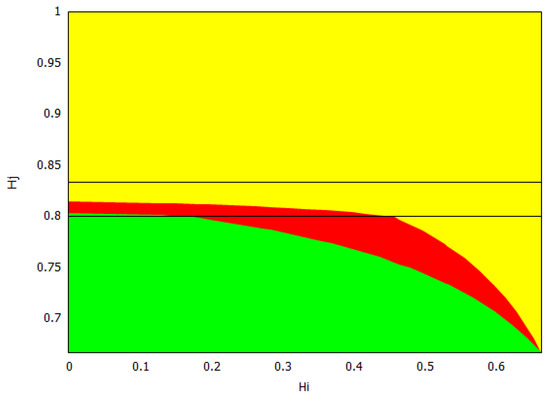
Figure 1. The welfare game type: Green—${\mathbf{L}}_j{\mathbf{W}}_i$; Red—PD; Yellow—${\mathbf{L}}_i{\mathbf{W}}_j$. Reproduced from [27].

For the welfare of the countries, we found two thresholds for the home production index $H_j$: the social-monopoly threshold $5/6$ and the social free-tariff threshold $4/5$ (see Figure 1). For both countries, the social tariffs are lower than the Nash tariffs, and they are lower for both countries except when $H_j\ge 5/6$, where $X_j$ blocks imports in both situations. Thus, any trade agreement that enforces the social tariffs will therefore lower the tariffs used at a competitive (Nash) equilibrium. For all the values of the home production indexes $H_i$ and $H_j$, country $X_i$ always chooses the Nash tariff $A_{W,i}$ and its tariff vanishes at the social optimum.

When $H_j$ is above the social-monopoly threshold $5/6$, then country $X_j$ blocks imports by setting the maximal tariff $T_j$ at both the Nash and social, and hence in its own market, there is a monopoly by its home firm. Furthermore, the game is of ${\mathbf{L}}_i{\mathbf{W}}_j$ type, and country $X_j$ has a welfare gain. When $H_j$ is below the social-monopoly threshold $5/6$, the game has three possible outcomes: the prisoner’s dilemma PD or both types of lose–win: ${\mathbf{L}}_i{\mathbf{W}}_j$ and ${\mathbf{L}}_j{\mathbf{W}}_i$. In this case, the Nash tariff for country $X_j$ is $A_{W,j}$. If $4/5<Hj<5/6$ its social tariff is $B_{W,j}$, and if $2/3<Hj\le 4/5$, its social choice is to make its tariff disappear. We observe from Figure 1 that when the index $H_j$ is between the two thresholds, the majority of the parameters yield either a PD or a ${\mathbf{L}}_i{\mathbf{W}}_j$-type game. This means that country $X_j$ has a welfare gain except for a small parameter region where country $X_j$ has a welfare loss (${\mathbf{L}}_j{\mathbf{W}}_i$). When $H_j$ is lower and closer to $2/3$ (this means that the home production of $X_j$ is lower in comparison to the home quantity in a monopoly situation), it becomes more likely that the game type is ${\mathbf{L}}_j{\mathbf{W}}_i$ with country $X_j$ losing welfare. For lower values of $H_i$, $H_j$ does not need to be so low to have a lose–win ${\mathbf{L}}_j{\mathbf{W}}_i$-type game, and there is a threshold in $H_i$ (approximately $0.2$) such that the game is always of this type when $H_j$ is below the social free-tariff threshold. Even for low values of $H_i$, if the index $H_j$ of country $X_j$ is sufficiently big, i.e., the eventual loss in the ratio that defines $H_j$ is small, then the game is of ${\mathbf{L}}_i{\mathbf{W}}_j$ type, and so country $X_j$ wins welfare. Observe that in this case, due to this greater competitiveness of $X_j$, it is better at the social optimum for $X_j$ to choose its maximal tariff and block imports and so be monopolistic in its market.

We remark that all the frontiers of the three regions leave from the corner $(H_i,H_j)=(2/3,2/3)$. This observation makes sense once we study this corner separately. In this case, we have $H_i=2/3=H_j$, so we have that $T_i^{*}=T_i$ and $T_j^{*}=T_j$ which only depends on the maximal tariffs and the game has three outcomes: (1) If the maximal tariffs $T_i$ and $T_j$ are sufficiently close to each other (more precisely $T_j/T_i\in [3/4,4/3]$), the game is of Prisoner’s dilemma (PD) type; (2) when one of the maximal tariffs, say $T_i$, is sufficiently larger than the other maximal tariff, $T_j$, (more precisely $T_j/T_i<3/4$), the outcome is ${\mathbf{L}}_i{\mathbf{W}}_j$; (3) when $T_j$ is sufficiently larger than $T_i$ (more precisely $T_j/T_i>4/3$), the outcome is ${\mathbf{L}}_j{\mathbf{W}}_i$.

3. Nash and Social Shares

In this section, we graphically define and describe the shares of welfares, profits and consumer surpluses of the countries at the Nash and social tariffs that will be important for our subsequent analysis.

In absolute terms, if the two countries decide to impose the cooperative tariffs, the following hold: (a) the custom revenue of country $X_i$ vanishes, since their social optimum tariff vanishes, and in some situations it also vanishes for country $X_j$; when it does not vanish for country $X_j$ (occurring only for values of home production index $H_j$ between the two thresholds), then it can increase or decrease; (b) the consumer surplus of the countries always increases; and (c) the profits of the firms may increase or decrease.

Perhaps more important than the absolute value of gains or losses in these economic quantities are the relative shares of these quantities. For instance, even if the consumer surplus always increases, the relative share of the consumer surplus may change with the application of the social tariffs, thus resulting in a change in the balance between the two countries, since a dominant country in one aspect may cease to be dominant when the social tariffs are enforced. Together with the shares, the values of the differences between the Nash and social shares of welfare and other quantities are also relevant to compare the two countries. For instance, the Nash social consumer surplus share difference and the Nash social profit share difference allow us to compare the relative advantage of one country over the other country between the Nash and social equilibrium from the perspective of the firm and the consumer, respectively.

Therefore, we will present in several Figures, the shares as well as the share differences (i.e., the difference between Nash and social shares) for each of these relevant economical quantities to exhibit their properties in terms of the home production indexes $(H_i,H_j)$ with

$$0<H_i\le 2/3\le H_j<1.$$

We will denote evaluation at the Nash tariffs by superscript N and at the social tariffs by superscript S. We will denote the joint or total quantity of the two countries by subscript T.

Thus, the joint Nash welfare is $W_T^N=W_i^N+W_j^N$ and the joint social welfare is $W_T^S=W_i^S+W_j^S$. The Nash welfare share and the social welfare share are

$$Sh{W}_j^N=\frac{W_j^N}{W_T^N}\mathrm{and}Sh{W}_j^S=\frac{W_j^S}{W_T^S}.$$

(13)

Thus, $Sh{W}_i^N+Sh{W}_j^N=1$ and $Sh{W}_i^S+Sh{W}_j^S=1$. The Nash social welfare share difference is

$$\Delta Sh{W}_j=Sh{W}_j^N-Sh{W}_j^S,$$

(14)

and so $Sh{W}_j^N=Sh{W}_j^S+\Delta Sh{W}_j^S$ and $\Delta Sh{W}_j=-\Delta Sh{W}_i$.

Similarly, we define the Nash consumer surplus share and the social consumer surplus share

$$ShC{S}_j^N=\frac{C{S}_j^N}{C{S}_T^N}\mathrm{and}ShC{S}_j^S=\frac{C{S}_j^S}{C{S}_T^S}.$$

(15)

The Nash social consumer surplus share difference is

$$\Delta ShC{S}_j=ShC{S}_j^N-ShC{S}_j^S.$$

(16)

The Nash profit share and the social profit share are defined by

$$Sh{\pi }_j^N=\frac{{\pi }_j^N}{{\pi }_T^N}\mathrm{and}Sh{\pi }_j^S=\frac{{\pi }_j^S}{{\pi }_T^S},$$

(17)

The Nash social profit share difference is defined by

$$\Delta Sh{\pi }_j=Sh{\pi }_j^N-Sh{\pi }_j^S.$$

(18)

The Nash custom revenue share is defined by

$$ShC{R}_j^N=\frac{C{R}_j^N}{C{R}_T^N}.$$

(19)

The social custom revenue share is either undefined because both countries have zero custom revenue, or it is equal to 0 for one country and 1 for the other country in the case when the home production index is between the two thresholds we described above, so we will not compute it.

We first focus on the special case $H_i=2/3=H_j$, which means that $T_i^{*}=T_i$ and $T_j^{*}=T_j$, and so only depends on the maximal tariffs. It can be easily seen that this means that $c_i=c_j$, i.e., the firms in each country have the same production costs. The Nash and social welfare shares are given by

$$Sh{W}_j^N=\frac{63T_j^2+2T_i^2}{65(T_j^2+T_i^2)}\mathrm{and}Sh{W}_j^S=\frac{3T_j^2+T_i^2}{4(T_j^2+T_i^2)},$$

and the Nash social welfare share difference is

$$\Delta Sh{W}_j=\frac{57(T_j-T_i)(T_j+T_i)}{260(T_j^2+T_i^2)}.$$

The Nash and social profit shares are

$$Sh{\pi }_j^N=\frac{16T_j^2+T_i^2}{17(T_j^2+T_i^2)}\mathrm{and}Sh{\pi }_j^S=\frac{1}{2},$$

and the Nash social profit share difference is

$$\Delta Sh{\pi }_j=\frac{15(T_j-T_i)(T_j+T_i)}{34(T_j^2+T_i^2)}.$$

The Nash and social consumer surplus shares are

$$ShC{S}_j^N=ShC{S}_j^S=\frac{T_j^2}{T_j^2+T_i^2}.$$

hence, the Nash social consumer surplus share difference is

$$\Delta ShC{S}_j=0$$

The Nash custom revenue share is

$$ShC{R}_j^N=\frac{T_j^2}{T_j^2+T_i^2}.$$

The Nash and social welfare shares exhibit similar behaviours with both shares being higher for bigger values of $T_j$. However, for the Nash welfare share, its maximum value is 1, while for the social welfare share, the maximum is $0.75$. The Nash profit share is higher for bigger values of $T_j$ and its maximum value is $16/17$. The social profit share is equal to $1/2$, meaning that at the social tariffs. profit is evenly split between the two firms. The Nash social welfare share difference and the Nash social profit share difference are, respectively, between $-50/260$ and $50/260$ (approximately $19\%$), and between $-15/34$ and $15/34$ (approximately $44\%$). They are 0 along the line $T_i=T_j$, and when $T_i>T_j$, country $X_i$ has a positive share difference, while for $T_i<T_j$ country $X_j$ has a positive share difference. The Nash and social consumer surplus shares are the same, and so there is no change in consumer surplus when changing to cooperative tariffs. Both are equal to the Nash custom revenue share. These shares are higher for bigger values of $T_j$ and its maximum is 1.

In Figure 2, Figure 3 and Figure 4, we show the Nash and social share for the welfares, the profits and the consumers surplus. We see that there are low values of $H_i$ with the following properties: (a) the Nash and social welfares, profits and consumer surpluses shares of country $X_j$ are higher than $1/2$; (b) country $X_j$ is the looser in the game type for low values of $H_j$ and country $X_i$ is the looser in the game type for high values of $H_j$. We also have that there are high values of $H_i$ with the following properties: (a) the Nash and social welfares, profits, and consumer surpluses shares of country $X_i$ are higher than $1/2$; (b) country $X_i$ is the loser.

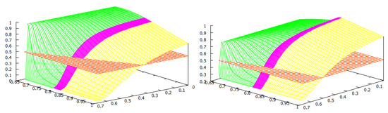
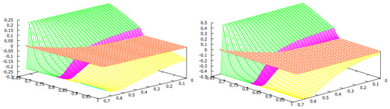
Figure 2. Left: The Nash welfare share $Sh{W}_j^N$ of country $X_j$. Right: The social welfare share $Sh{W}_j^S$ of country $X_j$. See Equation (13).

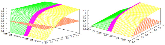
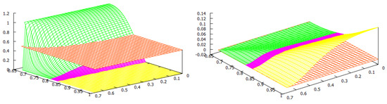
Figure 3. Left: The Nash profit share $Sh{\pi }_j^N$ of country $X_j$. Right: The social profit share $Sh{\pi }_j^S$ of country $X_j$. See Equation (17).

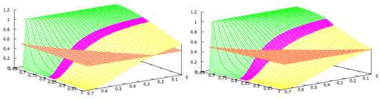
Figure 4. Left: The Nash consumer surplus share $ShC{S}_j^N$ of country $X_j$. Right: The social consumer surplus share $ShC{S}_j^S$ of country $X_j$. See Equation (15).

The Nash and social welfare, profit, and consumer surplus shares show similar qualitative features but significantly different quantitative properties (see Figure 2, Figure 3 and Figure 4). For all these shares: (a) for low values of $H_i$, the shares are higher for country $X_j$; (b) for high values of $H_i$ and high values of $H_j$, the shares are higher for country $X_i$; and (c) for high values of $H_i$ and low values of $H_j$, both cases occur. The isocurves of equal share ($0.5$) are close to segment lines starting at point $(2/3,2/3)$ but finishing at different points: for the Nash welfare, it finishes close to the point $(2/3,1)$; for the social welfare, it finishes close to the point $(0.5,1)$; for the Nash consumer surplus, it finishes close to the point $(0.2,1)$; for the social consumer surplus, it finishes close to the point $(0,1)$; for the Nash profits, it finishes close to the point $(0.5,1)$. For the custom revenue, the situation is different, as the isocurve is not close to being a straight line and it finishes at point $(0,7/9)$. The social profit share of country $X_j$ is always at least $0.5$, i.e., bigger than country $X_j$. It attains its minimum $0.5$ at the segment lines $H_i=2/3$ and $H_j=2/3$, and attaining its maximum 1 at the segment line with endpoints $(0,5/6)$ and $(0,1)$. Even when country $X_j$ has a lower Nash profit share, its share difference goes up to $50\%$ and it ends up with more than $50\%$ in social profit share.

The Nash social welfare share difference and the Nash social profit share difference show similar qualitative features but significantly different quantitative properties (see Figure 5). All the isocurves (0) corresponding to equal Nash and social shares are in the prisoner’s dilemma region or close to it and start at the point $(2/3,2/3)$. However, the Nash social welfare share difference isocurve (0) finishes close to $(0,0.81)$, more precisely, between $0.81$ and $0.815$, and the Nash social profit share difference isocurve (0) finishes close to $(0,5/6)$. The Nash social welfare share difference varies approximately between $-0.25$ and $0.25$, and the Nash social profit share difference varies approximately between $-0.5$ and $0.5$. The Nash social consumer surplus share difference is qualitatively different from the previous two share differences since it is always positive. The Nash social consumer surplus share difference for country $X_j$ varies approximately between 0 and $0.15$. The ${\mathbf{L}}_j{\mathbf{W}}_i$ and the prisoner’s dilemma PD regions can be noticed as corresponding to lower values of the Nash social consumer surplus share difference for country $X_j$ (see Figure 6).

Figure 5. Left: The Nash social welfare share difference $\Delta Sh{W}_j$ of country $X_j$ with respect to the welfare Nash and social tariffs. Right: The Nash social profit share difference $\Delta Sh{\pi }_j$ of country $X_j$. See Equations (14) and (18).

Figure 6. Left: The Nash custom revenue share $ShC{R}_j^N$ of country $X_j$. Right: The Nash social consumer surplus share difference $\Delta ShC{S}_j$ of country $X_j$. See Equations (19) and (16).

4. Welfare-Balanced International Trade Agreements and Shares

In this section, we indicate and describe some of the positive and negative effects of a welfare-balanced international trade agreement between the two countries. We also describe some possible remedies to these effects.

Let $\Delta W_T$ be the difference between the joint welfare computed at the social equilibrium and the joint welfare at the Nash equilibrium

$$\Delta W_T=W_T^S-W_T^N.$$

(20)

A $\gamma$-trade agreement determines the following $\gamma$-payoffs $V_i$ and $V_j$ for the countries $X_i$ and $X_j$:

$$\begin{array}{cc}\hfill V_i& =W_i^N+\gamma \Delta W_T\hfill \\ \hfill V_j& =W_j^N+(1-\gamma )\Delta W_T.\hfill \end{array}$$

(21)

where $\gamma$ is the countries’ bargaining power index and $\Delta W_T$ is the trade agreement welfare gain.

Let the trade agreement index be

$$g=g(H_i,H_j)=\frac{W_T^S}{W_T^N}.$$

(22)

For the welfare-balanced bargaining power index

$${\gamma }^N=\frac{W_i^N}{W_T^N},$$

(23)

the ${\gamma }^N$-payoffs of the welfare-balanced trade agreement are

$$\begin{array}{cc}\hfill V_i^N& =g{W}_i^N\hfill \\ \hfill V_j^N& =g{W}_j^N.\hfill \end{array}$$

(24)

The total welfare of the trade agreement is the total social welfare:

$$V_i^N+V_j^N=W_T^S.$$

(25)

The compensations associated with the trade agreement in order to maintain the welfare shares, in units of the welfare of the trade agreement, i.e., in total social welfare units, are given by the share differences:

$$\begin{array}{cc}\hfill \frac{V_i^N-W_i^S}{W_T^S}& =\Delta Sh{W}_i\hfill \\ \hfill \frac{V_j^N-W_j^S}{W_T^S}& =\Delta Sh{W}_j.\hfill \end{array}$$

(26)

The welfare-balanced trade agreement has the following features: (a) the two countries impose the welfare social tariffs; (b) the two countries attain joint welfare at the social optimum that is $g>1$ times higher than the joint Nash equilibrium welfare; (c) the joint social welfare is split in such a way that both countries maintain the same welfare shares that they had at the competitive tariffs. The country with a positive Nash social welfare share difference must be indemnified by the other country. The amount of this compensation in units of the total welfare of the trade agreement (i.e., in units of the joint social welfare) is determined exactly by the Nash social welfare share difference. See Figure 5. Thus, in the positive region, $\Delta Sh{W}_j>0$, $X_j$ is compensated by $X_i$ and in the negative region, $\Delta Sh{W}_j<0$, $X_j$ compensates $X_i$.

Plotting the values of the trade agreement index g, we see that it attains lower values for values of $(H_i,H_j)$ in the PD prisoner’s dilemma region or close to the prisoner’s dilemma region, and it attains higher values away from the prisoner’s dilemma region (see Figure 7), namely in the asymmetrical LW regions. The trade agreement index attains its maximum (approximately $1.22$) near the corner $(0.37,1)$. Hence, in the region where the game is of prisoner’s dilemma-type, or where it is close to prisoner’s dilemma (albeit all difficulties that may arise to achieve a welfare-balanced trade agreement), the gain will be lower than in other regions away from the prisoner’s dilemma region. On the other hand, higher gains are attained in the asymmetric regions.

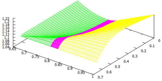
Figure 7. The trade agreement index g. See Equation (22).

The two countries enforce the social tariffs, so each country obtains the social profits, consumer surplus and custom revenue. This may cause some collateral effects on the economies of these countries. For instance, its produced quantities may change so that one of the countries is no longer the dominant force in terms of output. This influences other economic quantities such as profits, consumer surplus and custom revenue. These effects, which we may call the externalities of the trade agreement, are decisive with regard to whether the country signs the trade agreement, in the sense that the country may consider that the welfare compensation stated above is not sufficient to outweigh such collateral effects. Possible effects might include, for instance, increasing unemployment in the country due to a decrease in production, and a subsequent wave of migration from that country to the other, or the effect of a decrease in the profits of firms, which may cause firms to invest abroad, also possibly triggering the problem of unemployment in the home country. Other consequences may be a fall in the consumer’s surplus of one country relative to the other country, and a fall in revenues from using tariffs. Countries may try to mitigate and overcome these difficulties by including other features (that we do not explore in this work) in the trade agreement apart from the welfare compensation. For example, these features may be financing to the industry of the impaired country; R&D exchange between countries; compensation and investment in other sectors of the economy of the impaired country; etc.

In light of this, we identify and analyse the parameter regions where these difficulties occur. More precisely, these are the regions where the relevant economics we have considered above, such as profits, consumer surplus and custom revenue are such that the social shares are higher for one country while the Nash shares are higher for the other country. When this occurs, then there is a change in the dominant force concerning that economic quantity, and these externalities are a disincentive for that country to sign the trade agreement and might cause that country to not sign it, even in situations where it is compensated in welfare by the other country as ruled by the welfare-balanced trade agreement. Another situation that may occur is that one of the countries may have benefit in some economic quantity when the social tariffs are put into practice, but simultaneously have to indemnify the other country. Thus, the country must perform a thorough analysis of the consequences to know whether that benefit is worthwhile compared to the obligation of compensating the other country.

In Figure 8, we plot all the isocurves for the share differences (0), the Nash shares and the social shares ($0.5$). The violet region is delimited by the isocurve of the Nash custom revenue share. The blue region is delimited from the grey region by the isocurve of the Nash social welfare share difference, and the grey region is delimited from the yellow region by the isocurve of the Nash social profit share difference. From the yellow region, we have the brown, cyan, black, pink, and orange regions which are, respectively, delimited by the isocurve of the social consumer surplus share; the isocurve of the Nash consumer surplus share; the isocurve of the Nash welfare share; the isocurve of the Nash profit share; and the isocurve of the social welfare share.

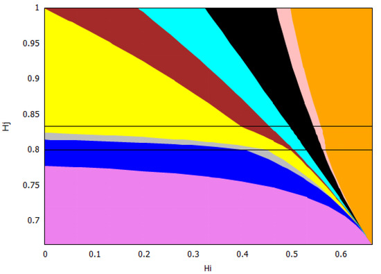
Figure 8. The Nash share isocurves, the social share isocurves, (i.e., $=0.5$) and the share difference isocurves, (i.e., $=0$) for welfare, profit, consumer surplus and custom revenue.

The relation of the isocurves with the frontiers of the LW and PD regions presented in Figure 1 is relatively complex. The violet and blue regions are completely contained in the union of the ${\mathbf{L}}_i{\mathbf{W}}_j$ and PD regions. The grey region intersects the three game-type regions. The PD region is not contained in the grey region and below. In Figure 9, we represent the decomposition of the PD region according to the violet, blue and grey regions, and in red is the portion of the PD that lies outside of the union of the violet, blue and grey regions. The upper frontier of the PD region enters through the grey region and finishes just above the frontier between the blue and grey regions. It always remains above the blue region since the blue region never intercepts the ${\mathbf{L}}_i{\mathbf{W}}_j$ region. Furthermore, the violet region is almost totally inside the ${\mathbf{L}}_j{\mathbf{W}}_i$ region, except for a small portion that is of PD type, as represented in the left Figure. Regarding the other regions, we first observe that the brown, cyan, black, pink and orange regions do not intercept the ${\mathbf{L}}_i{\mathbf{W}}_j$ regions. This means that in these regions, country $X_i$ is always a winner in terms of absolute welfare. They do intercept the PD regions, although the parameter region for which this occurs is very small, as we show in Figure 9.

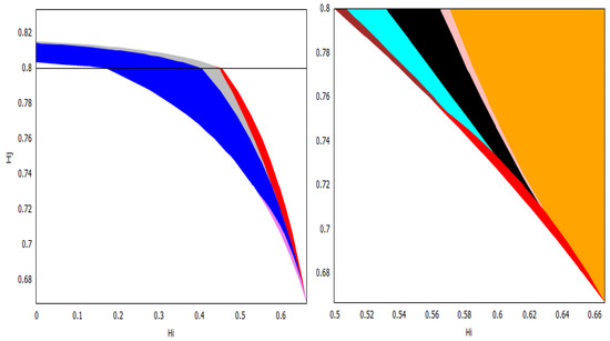
Figure 9. Left: The decomposition of the PD region according to the violet, blue and grey regions; Right: In red, the portion of the brown, cyan, black, pink and orange regions that intersects the PD region.

Since the trade agreement is based on the welfare of the two countries, we start by analysing the welfare. The Nash welfare share of country $X_j$ is higher than that of $X_i$ in and below the cyan region. The social welfare share is higher for country $X_j$ except in the orange region. The Nash social welfare share difference of country $X_j$ is negative above the union of the violet and blue regions. Hence, in this region, by the welfare-balanced trade agreement, country $X_j$ must compensate $X_i$, but since the welfare-balanced trade agreement maintains the Nash welfare share, it still has a higher welfare share up to the cyan region. In the union of the black, pink, and orange regions, country $X_i$ is compensated and retains its higher welfare share. The advantage of the welfare-balanced trade agreement is that country $X_i$ remains with a higher welfare share not only in the orange region, but also in the pink and black regions where it had a higher Nash welfare share but a lower social welfare share. In and below the blue region, country $X_j$ has a positive Nash social welfare share difference and so is compensated by $X_i$ and it has a higher welfare share. When the game type is ${\mathbf{L}}_i{\mathbf{W}}_j$ or ${\mathbf{L}}_j{\mathbf{W}}_i$ the country that has a loss in absolute welfare also has a loss in share and so is compensated by the other country in the welfare-balanced trade agreement. When the game type is $\mathbf{PD}$, so that both countries have an absolute gain, then the Nash social share difference can be positive or negative, so country $X_j$ may be asked to indemnify $X_i$ or may be indemnified by $X_i$. Furthermore, we observe that, in most of the union of the violet and blue regions, (i.e., the region where country $X_j$ is indemnified in its welfare by country $X_i$) country $X_j$ is also the loser (${\mathbf{L}}_j{\mathbf{W}}_i$). This might induce a greediness effect in country $X_j$ (and even more so in the violet region because of its higher Nash custom revenue share, which is lost when the social tariffs, which are the enforced zero tariffs) which may reflect itself in the preference of $X_j$ for a bargaining power index that is more favourable to it, i.e., a $\gamma$ smaller than g, which may eventually render the welfare-balanced trade agreement unstable. However, when $H_j$ gets closer to $2/3$, the values of g increase slightly, improving the advantage of the agreement and perhaps working as an incentive for its enforcement.

Regarding the custom revenue isocurves, we have that in the violet region country $X_j$ has a higher Nash custom revenue share than country $X_i$. At the social optimum, country $X_i$ always gives up its custom revenue in favour of going tax-free, which improves its consumer surplus in absolute terms and in terms of its share, as we will see below. Country $X_j$ does not apply tariffs in the region below the social tax-free threshold but prefers to apply the maximal tax in the region above the social monopoly-tax threshold, not allowing $X_i$ to export both at the Nash and the social optimum. It makes its tariff move from 0 to the maximal tariff in between these two regions, with this being the only region where there is a positive custom revenue at the social optimum for one of the countries, in the case of country $X_j$ (and their share is 1). As a result, for values of $H_j$ between these two thresholds, country $X_j$ has some positive revenue, which may be important for their decision to sign the trade agreement or not, since it may be seen as an advantage against, for instance, the compensation that it must give to the other country, which occurs outside the blue region, or the loss in share profit that occurs in the grey region, or in the brown region where their Nash consumer surplus share is higher than $X_i$’s, but their social share is not. As noted before, the violet region is contained in the union of the ${\mathbf{L}}_j{\mathbf{W}}_i$ and $\mathbf{PD}$ regions, so, in absolute terms regarding welfare, country $X_i$ is a winner, or equivalently, in the ${\mathbf{L}}_i{\mathbf{W}}_j$ region, country $X_j$ has a lower Nash custom revenue share. We observe that country $X_j$ can have a lower share within the ${\mathbf{L}}_j{\mathbf{W}}_i$ region.

The Nash consumer surplus share of country $X_j$ is higher than that of country $X_i$ in and below the brown region. The social consumer surplus share of country $X_j$ is higher than that of $X_i$ in and below the yellow region. We have previously observed that the consumer surplus increases for both countries when the social tariffs are applied. In spite of this increase in absolute terms, the Nash social consumer surplus share difference of country $X_j$ is always positive (see Figure 6), meaning that their share of consumer surplus at the Nash equilibrium is bigger than at the social optimum. This loss is at most approximately $0.14$. This mainly occurs because country $X_j$ exports more since country $X_i$ is tariff-free at the social optimum, thus increasing the consumer surplus of $X_i$. For $H_j$ above the social monopoly threshold $5/6$, $X_i$ does not export and the consumer surplus of $X_j$ remains the same, hence its share diminishes. For other home production indexes of country $X_j$, we have that country $X_i$ also exports more since the tariffs are lowered, but $X_j$ only goes tariff-free for $H_j$ below the tariff-free threshold $4/5$, and so their consumer surplus also increases, but in both situations, their share diminishes.

For regions above the brown, country $X_j$ already has a lower share than $X_i$ at the Nash equilibrium and will obtain an even lower share with the trade agreement. In the brown region, $X_j$ has a higher share at the Nash equilibrium, but no longer has an advantage at the social optimum. In the yellow regions and below, country $X_j$ has a bigger share at the Nash equilibrium, and in spite of the loss in share, he still has a higher social share. In the regions where $X_j$ has a lower social share, that is, in and above the brown regions, the trade agreement rules that he indemnifies $X_i$. This might be a difficulty for country $X_j$, which might have to use its custom revenue (that is positive for $H_j$ between the two thresholds as we noted above), or somehow use the increase in the profits share in these regions (which occur since they lie above the grey region), possibly through taxation, as well the fact that its firm always has the most of the joint profits of the two countries at the social optimum.

Regarding this last observation, we now analyse the profit shares. The Nash profit share of country $X_j$ is higher than that of country $X_i$ in and below the black region and it is lower in the union of the pink and orange regions. The social profit share of country $X_j$ is always bigger for country $X_j$ (see Figure 3). The Nash social profit share difference of country $X_j$ is always negative above the grey region, so the profit share increases with the use of social tariffs. For this region, the game type is ${\mathbf{L}}_i{\mathbf{W}}_j$ except for the small red region in Figure 9 where the game type is $\mathbf{PD}$, so $X_j$ always has a gain in absolute welfare. In these regions, the trade agreement presents an advantage for the firm of country $X_j$, since it increases its profit share. In the yellow, brown, cyan, and black regions, country $X_j$ has a higher profit share and reinforces its position with the trade agreement, obtaining a higher share. The advantage for the firm is also evident in the pink and orange regions, where the firm of $X_j$ is not the dominant firm in terms of Nash profit share but does become dominant with the trade agreement. However, in these regions, country $X_j$ has to compensate country $X_i$ according to the trade agreement. Because of this, the country might have to impose taxes on the profits of the firms to fulfil the trade agreement. In the yellow, brown and cyan regions, after the compensation, $X_j$ has a higher welfare share. In the black, pink, and orange regions, he has no such advantage in welfare share. In and below the grey region, country $X_j$ has a decrease in profit share but always has a higher social share. In the blue and violet regions, country $X_j$ is indemnified by country $X_i$. This compensation may be used by the country to compensate for the loss of the profit share of its firm by investing in it. In the grey region, the opposite occurs, and country $X_j$ has to indemnify $X_i$. In this case, he may need to use its custom revenue, or tax the profits to indemnify $X_i$. This might prove difficult for the country, since in the grey region, the firm faces a decline in its profit share (although it is still the dominant firm).

We observe that, in the ${\mathbf{L}}_j{\mathbf{W}}_i$ region, meaning that country $X_j$ is a loser in absolute terms, it has a higher Nash welfare, profit and consumer surplus shares. This occurs for a wider region since when country $X_j$ is indemnified by $X_i$ (which occurs below the blue region), it has an advantage in Nash shares in all these quantities: welfare, profits and consumer surplus. In these regions, country $X_j$ also has a higher social profit and consumer surplus shares, so, with the use of the social tariffs, it also is the dominant country in consumer surplus and has the dominating firm. If the trade agreement is not balanced and just applies the social tariffs, it would remain the dominant country in terms of welfare, since its social welfare share is higher than $X_i$’s in this region. Hence, country $X_i$ (which is the country with the greatest decline in home production in a tax-free situation, since $H_i$ is lower than $H_j$) cannot simultaneously be a winner and have higher shares. This advantage of $X_j$ in all shares occurs up to the frontier of yellow and brown regions. However, when the game type is ${\mathbf{L}}_i{\mathbf{W}}_j$, then the Nash and social welfare, consumer surplus shares and the Nash profit share of country $X_j$ may be higher or lower than those of $X_i$. These shares are higher for $X_i$ for higher values of $H_i$ and lower when $H_i$ is lower. When $H_j$ increases, then $H_i$ does not need to be so high to assure higher shares for country $X_i$. For the Nash custom revenue share, the situation is different since in the ${\mathbf{L}}_j{\mathbf{W}}_i$ and PD regions, country $X_i$ can have a higher share than country $X_j$. However, in the ${\mathbf{L}}_i{\mathbf{W}}_j$ region, it always has the lower Nash custom revenue share.

If the Nash social welfare share difference or the Nash social consumer surplus share difference or the Nash social profit share difference is large, then the countries have to be very careful in making a trade agreement because small differences in the trade agreement can mean significant social and economic changes for the countries. For values of $(H_i,H_j)$ in the prisoner’s dilemma region or close to the prisoner’s dilemma region, the Nash social welfare share difference, the Nash social consumer surplus share difference, and the Nash social profit share difference have lower values than they do away from the prisoner’s dilemma region (see Figure 5 and Figure 6). For instance, when $H_j$ gets closer to $2/3$, the welfare compensation that $X_i$ has to give to $X_j$ increases, making the agreement riskier for $X_j$. This compensation may go up to $25\%$ of the joint social welfare, making the agreement very relevant because of the magnitude of the associated compensations, but also very difficult to establish because of this magnitude and the large changes that may exist in the share of the profits of the firms as well as in the consumer surplus of a country.

5. Conclusions

We considered an international trade model with two countries and two stages. In the first stage of the game, governments impose their tariffs on imports from the other country. In the second stage of the game, firms in each country choose their home and export quantities competitively in a Cournot–type game. In the tariffs sub-game (first stage game) between governments, they can choose competitive tariffs (Nash) or cooperative tariffs (social) to maximise their joint welfare.

In this context, we proposed and analysed a welfare-balanced trade agreement between the two countries. In such an agreement, the social cooperative tariffs are enforced and the cooperative aggregate welfare of the countries is distributed in a way such that the relative shares of welfare between the two countries are maintained. We discussed some of the effects that present major difficulties for the establishment of the welfare-balanced trade agreement by both parties, and the parameter regions where they occur. These effects are measured through changes in the relative shares of the countries regarding quantities such as the firm’s profits, consumer’s surplus and custom revenues when the cooperative social tariffs are enforced instead of the competitive Nash equilibrium tariffs. We have analysed the gains of the trade agreements through the trade agreement index that we explicitly computed and analysed.

The following questions, among others, can be raised about the trade agreement: (a) what additional measures should be part of the trade agreement to mitigate the negative externalities of the country that has a decrease in its production and/or the profits of its firm, its custom revenue or the surplus of its consumers. These measures may include an R&D swap between both countries and financing to industry and other sectors, among others. We note that countries that can make balanced trade agreements in more than one economic sector such that the total compensation of the agreements is not relevant might be in a better position to negotiate; (b) what additional measures should be part of the trade agreement to force both countries to agree to set the social tariffs in such a way that the agreement is theoretically durable and sustainable in time, preferably rendering it self-enforcing.

The main contribution from the present work is the analysis of the effects regarding the aforementioned economic quantities. They play a very relevant role in the establishment of the trade agreement. More precisely, in the context of this standard classic model, the establishment of the welfare-balanced trade agreement might be very difficult since it may change the country’s relative position in terms of production, consumption, or both.

The present study has an obvious limitation in that the international trade model under consideration is a very simplified and unrealistic one, with only two countries and one firm in each country producing the same good. On the one hand, it allows a full description of the economic quantities of the model, but it shows significant complexity driven by the interplay between these quantities. Our main conclusions and observations concern the complexity and difficulty of the prediction and analysis of international trade outcomes.

Future work can consist, for instance, in introducing some of the features mentioned above, such as studying conditions for the self-enforcing of the agreement, studying the effects of R&D investment sharing and swapping between the two firms to decrease their production costs, foreign industrial investment, merging and shutting-down of firms, the effects of subsidies, fines and other types of transfers between countries. The inclusion of some of these features into the trade agreement may be a way to overcome some of the externality effects that we discussed throughout the paper.

References

- McMillan, J. Game Theory in International Economics; Harwood Academic Publishers: Chur, Switzerland, 1986. [Google Scholar] [CrossRef]
- von Haberler, G. The Theory of International Trade with Its Application to Commercial Policy; Macmillan: New York, NY, USA, 1937; Available online: https://mises.org/library/international-trade (accessed on 26 September 2022).
- Brander, J.A. Strategic trade policy. In Handbook of International Economics; Elsevier: Amsterdam, The Netherlands, 1995; Volume 3, Chapter 27; pp. 1395–1455. [Google Scholar] [CrossRef]
- Dixit, A. Strategic aspects of trade policy. In Advances in Economic Theory; Bewley, T., Ed.; Cambridge University Press: Cambridge, UK, 1987; Chapter 9; pp. 329–362. [Google Scholar] [CrossRef]
- Spencer, B.J.; Brander, J.A. International R&D Rivalry and Industrial Strategy. Rev. Econ. Stud. 1983, 50, 707–722. [Google Scholar] [CrossRef]
- Brander, J.A.; Spencer, B.J. Export subsidies and international market share rivalry. J. Int. Econ. 1985, 18, 83–100. [Google Scholar] [CrossRef]
- Liao, P.C. Rivalry between exporting countries and an importing country under incomplete information. Acad. Econ. Pap. 2004, 32, 605–630. [Google Scholar]
- Dixit, A.; Grossman, G.M. Targeted export promotion with several oligopolistic industries. J. Int. Econ. 1986, 21, 233–249. [Google Scholar] [CrossRef]
- Grossman, G.M. Strategic export promotion: A critique. In Strategic Trade Policy and the New International Economics; Krugman, P., Ed.; MIT Press: Cambridge, MA, USA, 2007; Chapter 3; pp. 47–68. [Google Scholar]
- Bagwell, K.; Staiger, R.W. A Theory of Managed Trade. Am. Econ. Rev. 1990, 80, 779–795. [Google Scholar]
- Helpman, E. Increasing Returns, Imperfect Markets, and Trade Theory. In Handbook of International Economics Volume I; Jones, R.W., Kenen, P.B., Eds.; North Holland Press: Amsterdam, The Netherlands, 1984; Chapter 7; pp. 325–365. [Google Scholar] [CrossRef]
- Fisher, E.O.; Wilson, C.A. Price competition between two international firms facing tariffs. Int. J. Ind. Organ. 1995, 13, 67–87. [Google Scholar] [CrossRef][Green Version]
- Bulow, J.I.; Geanakoplos, J.D.; Klemperer, P.D. Multimarket Oligopoly: Strategic Substitutes and Complements. J. Political Econ. 1985, 93, 488–511. [Google Scholar] [CrossRef]
- Eaton, J.; Grossman, G.M. Optimal Trade and Industrial Policy Under Oligopoly. Q. J. Econ. 1986, 101, 383–406. [Google Scholar] [CrossRef]
- Dixit, A. International Trade Policy for Oligopolistic Industries. Econ. J. 1984, 94, 1–16. [Google Scholar] [CrossRef]
- Brander, J.A. Intra-industry trade in identical commodities. J. Int. Econ. 1981, 11, 1–14. [Google Scholar] [CrossRef]
- Krishna, K. Trade restrictions as facilitating practices. J. Int. Econ. 1989, 26, 251–270. [Google Scholar] [CrossRef]
- Staiger, R. International rules and institutions for trade policy. In Handbook of International Economics Volume III; Jones, R.W., Kenen, P.B., Eds.; North Holland Press: Amsterdam, The Netherlands, 1984; Chapter 29; pp. 1495–1551. [Google Scholar] [CrossRef]
- Bagwell, K.; Staiger, R.W. Enforcement, Private Political Pressure, and the General Agreement on Tariffs and Trade/World Trade Organization (GATT/WTO) Escape Clause. J. Leg. Stud. 2005, 34, 471–513. [Google Scholar] [CrossRef]
- Bagwell, K.; Staiger, R.W. An Economic Theory of GATT. Am. Econ. Rev. 1999, 89, 215–248. [Google Scholar] [CrossRef]
- Limão, N.; Saggi, K. Tariff retaliation versus financial compensation in the enforcement of international trade agreements. J. Int. Econ. 2008, 76, 48–60. [Google Scholar] [CrossRef][Green Version]
- Limão, N.; Saggi, K. Size inequality, coordination externalities and international trade agreements. Eur. Econ. Rev. 2013, 63, 10–27. [Google Scholar] [CrossRef]
- Kilolo, J.M.M. Country Size, Trade Liberalization and Transfers; MPRA Paper; University Library of Munich: Munich, Germany, 2013. [Google Scholar]
- Kilolo, J.M.M. Country asymmetry, trade agreements, and transfers. Econ. Politics 2021, 33, 37–51. [Google Scholar] [CrossRef]
- Banik, N.; Ferreira, F.A.; Martins, J.; Pinto, A.A. An Economical Model For Dumping by Dumping in a Cournot Model. In Dynamics, Games and Science II, DYNA 2008, in Honour of Maurício Peixoto and David Rand; Springer Proceedings in Mathematics; Peixoto, M.M., Pinto, A.A., Rand, D.A., Eds.; Springer: Berlin/Heidelberg, Germany, 2011; Volume 2, pp. 141–154. [Google Scholar] [CrossRef]
- Martins, J.; Banik, N.; Pinto, A.A. A Repeated Strategy for Dumping. In Discrete Dynamical Systems and Applications, ICDEA 2012; Springer Proceedings in Mathematics, & Statistics; Alseda, L., Cushing, J.M., Elaydi, S., Pinto, A.A., Eds.; Springer: Berlin/Heidelberg, Germany, 2016; Volume 180, pp. 145–153. [Google Scholar] [CrossRef]
- Martins, F.; Pinto, A.A.; Zubelli, J.P. Nash and social welfare impact in an international trade Model. J. Dyn. Games 2017, 4, 149–173. [Google Scholar] [CrossRef]
- Gibbons, R. A Primer in Game Theory; Pearson Prentice Hall: Hoboken, NJ, USA, 1999. [Google Scholar]
- Corchon, L.C. Trade and growth: A simple model with NOT-SO-Simple implications. J. Dyn. Games 2017, 4, 175–190. [Google Scholar] [CrossRef]
- Amir, R.; Jin, J.Y.; Troege, M. On the limits of free trade in a Cournot world: When are restrictions on trade beneficial? Can. J. Econ./Rev. Can. D’économique 2022. in print. [Google Scholar] [CrossRef]
- Bobrik, G.; Bobrik, P.; Sukhorukova, I. The sensitivity of commodity markets to exchange operations such as swing. J. Dyn. Games 2021, 8, 119–128. [Google Scholar] [CrossRef]
- Gibaud, S.; Weibull, J. The dynamics of fitness and wealth distributions—A stochastic game-theoretic model. J. Dyn. Games 2022, 9, 405–432. [Google Scholar] [CrossRef]
- Dokumacı, E.; Sandholm, W.H. Schelling redux: An evolutionary dynamic model of residential segregation. J. Dyn. Games 2022, 9, 373–403. [Google Scholar] [CrossRef]
Disclaimer/Publisher’s Note: The statements, opinions and data contained in all publications are solely those of the individual author(s) and contributor(s) and not of MDPI and/or the editor(s). MDPI and/or the editor(s) disclaim responsibility for any injury to people or property resulting from any ideas, methods, instructions or products referred to in the content. |
© 2022 by the authors. Licensee MDPI, Basel, Switzerland. This article is an open access article distributed under the terms and conditions of the Creative Commons Attribution (CC BY) license (https://creativecommons.org/licenses/by/4.0/).